Treefall Gap Mapping Using Sentinel-2 Images


1
Department of Surveying and Remote Sensing, Institute of Geomatics and Civil Engineering, Faculty of Forestry, University of Sopron, Sopron 9400, Hungary
2
Department of Geodesy and Geoinformation, Faculty of Mathematics and Geoinformation, Technische Universität Wien, 1040 Wien, Austria
*
Author to whom correspondence should be addressed.
Forests 2017, 8(11), 426; https://doi.org/10.3390/f8110426
Submission received: 27 September 2017
/
Revised: 25 October 2017
/
Accepted: 3 November 2017
/
Published: 7 November 2017
(This article belongs to the Special Issue New Application based on Advanced Remote Sensing Data in Forests and Wood Land Areas)
Abstract
:Proper knowledge about resources in forest management is fundamental. One of the most important parameters of forests is their size or spatial extension. By determining the area of treefall gaps inside the compartments, a more accurate yield can be calculated and the scheduling of forestry operations could be planned better. Several field- and remote sensing-based approaches are in use for mapping but they provide only static measurements at high cost. The Earth Observation satellite mission Sentinel-2 was put in orbit as part of the Copernicus programme. With the 10-m resolution bands, it is possible to observe small-scale forestry operations like treefall gaps. The spatial extension of these gaps is often less than 200 m2, thus their detection can only be done on sub-pixel level. Due to the higher temporal resolution of Sentinel-2, multiple observations are available in a year; therefore, a time series evaluation is possible. The modelling of illumination can increase the accuracy of classification in mountainous areas. The method was tested on three deciduous forest sites in the Börzsöny Mountains in Hungary. The area evaluation produced less than 10% overestimation with the best possible solutions on the sites. The presented work shows a low-cost method for mapping treefall gaps which delivers annual information about the gap area in a deciduous forest.
1. Introduction
Artificial treefall gaps [1] in a forest canopy are used during forest structure conversion [2] to form even-aged to uneven-aged forests. Foresters apply this assisted natural regeneration method typically in the foothill and montane zone of native deciduous forests, which have already entered their reproductive age in Hungary. There, each tree has roughly the same total height and breast height diameter (DBH). To create an artificial treefall gap, a group of trees within a diameter of approximately one tree height is selected to be harvested. In the literature, this method is often called “group selection” [3]. The tree removal creates a gap in the canopy layer. The purpose of this process is to regenerate the forest in that open area with young seedlings, preferably using seeds of the neighboring trees in a natural way of succession [4]. If there are no local seeds, foresters may artificially plant seedlings from a nursery in the gap. The idea of artificial treefall gaps is based on the forest dynamic where gaps are created by natural disturbances [5] like ice damage or windfall or when standing dead trees naturally topple. Each forest type requires different gap handling based on their sylvicultural properties. Generally, young trees require a lot of sunlight to germinate the seeds or grow [6]. Under the canopy, only diffuse illumination is available [7]. The gap in the canopy layer allows direct sunlight for the seedlings, which causes faster growth [8,9].
With this forest regeneration method, it is possible to have uneven-aged trees inside the forest compartment borders, providing continuous forest cover [10] without clear cuts. Thus treefall gaps have an important role in the ecosystem for maintaining the biodiversity and for influencing nutrient cycling, and preserving the uneven-age nature of late-successional forests [11]. Artificial gaps are opened according to a schedule during the sylvicultural management to ensure a continuous canopy cover [12]. Since the growth of deciduous natural forests in mountainous areas is relatively slow, the schedule of gap opening is influenced by ecological and economic factors. To make the scheduling optimal we need to know the dendrometric parameters [13] of the forest stand and size of the stand. For sustainable forest management, [14], it is necessary to be aware of the resources like the size of the standing forest and canopy gaps. Field-based sampling methods of forest mensuration like measuring basal area or using a volume table require the exact area of the forest stand to calculate forest biomass volume [15]. These two forest mensuration methods are the most frequently used at the study region to update forest inventory. In Hungary, there are more than 60,000 hectares of those even-aged forests which have to be transformed into uneven-aged by methods described above, according to the forest law [16]. In most cases the gap method is used. Forest managers have had detailed maps of forest compartments since the 19th century [17]. However, these maps ignore the sub-compartments like treefall gaps. There are only few cases where the area of these gaps is known [18,19,20]. A review has been published about the existing methodology for treefall gap determination [11]. According to the review, gaps can be described with two main parameters: their size and their age. Since gaps are created in a living ecosystem, their size changes through time. Therefore, their age is an important parameter. The crown projection area for a single tree is quite dynamic. It continuously changes around the gap, so continuous mapping is required. The size of a gap is usually determined by using the crown projections of the neighboring trees by surveying. Generally simpler field methods are used when the shape of the gap is modeled with a simple geometric shape. In that case, it is enough to measure diameters, although their shape is usually irregular. People survey gaps with geodetic methods only for research purposes. In practice, remote sensed aerial materials like orthophotos [21] and digital surface models are often used for gap mapping [22,23]. However the cost of these methods makes continuous mapping impracticable and therefore an alternative solution is needed which fulfills the frequent and sustainable requirements.
The high-resolution Earth Observation (EO) satellites are a low-cost alternative for remote sensed data, since they provide images with higher temporal resolution. The spatial resolution of a pixel (5–30 m) makes it possible to detect the existence of a gap inside the canopy on a pixel and sub pixel level. Sentinel-2 carries the Multispectral Instrument (MSI) sensor [24] which has 10, 20 and 60 m resolution bands. The blue (B2), green (B3), red (B4) and the near infra-red (NIR) (B8) 10 m resolution bands are feasible for the study area. The size of a gap in the study area is usually smaller than the 20-m pixel’s size, which results in a less reliable map. Though they contain important information about the red edge and the short-wave infrared spectra for the forest type [25], it is rare to use this kind of data for forest gap mapping. In certain cases, this data source has been used for treefall gap mapping. Garbarino et al. [26] used a very high resolution (VHR) Kompsat-2 image in Bosnia with an automated classification method and visual interpretation. In another study [27], a stereo VHR satellite image pair from WorldView-2 was used for gap mapping in a Ukrainian Beech forest. In that paper the 3D information from the stereo pair was also used during the automated classification of gaps. Negron-Juarez et al. [28] inspected the use of Landsat images for mapping treefall gaps in Middle-Amazonia. They used a spectral mixture analysis for their research.
The main objective of this study is to analyze the potential of Sentinel-2 images for treefall gap detection. The spectral signature of gaps must be investigated considering the illumination on their surfaces along with the application of a spectral unmixing method for mapping. Assuming that the different pre-processing levels of Sentinel-2 images are highly affecting the results, we aimed to analyze their influences on the archivable accuracies. The results were compared to VHR remotely sensed images and field data for validation. We assessed the accuracy of the workflow. Finally the benefit of the treefall gap maps for the forest management sector is analyzed.
2. Materials
2.1. Study Area
The study area is situated in the Börzsöny Mountains in the North Hungarian Range [29] north of the river Danube. The bedrock under the study sites is made of andesite agglomerates of the Miocene volcanism [30]. The higher (500–938 m a.s.l.) steep, rocky slopes and deep valleys of the northern part of the area extend in the lower elevations (300–500 m a.s.l.) as gentle slopes of the southern part [31]. The mean annual temperature is 8 °C; mean monthly temperature is −3.5 in January and 18 °C in July, and the annual precipitation is 550–900 mm [32,33]. Due to the very intensive exploitation of forests of Börzsöny mountains in the 19th Century, which was driven by the appearance of modern transport methods like trains [34], the age distribution of the forests is irregular [35]. Today, sustainable forest management is done by the state-owned Ipoly Erdő Zrt. Company(Balassagyarmat, Hungary). One of their main challenges is to transform the irregular distribution of age groups over the whole managed area into evenly distributed age groups by creating uneven-aged forests within a forest compartment.
Three distinct areas were chosen as study sites, which represent the mapping challenges with treefall gaps (Figure 1). One study area is covered by European beech (Fagus sylvatica L.) and the other two by sessile oak (Quercus petraea (Matt.) Liebl.).
2.1.1. Oak Study Site I. (OS1)
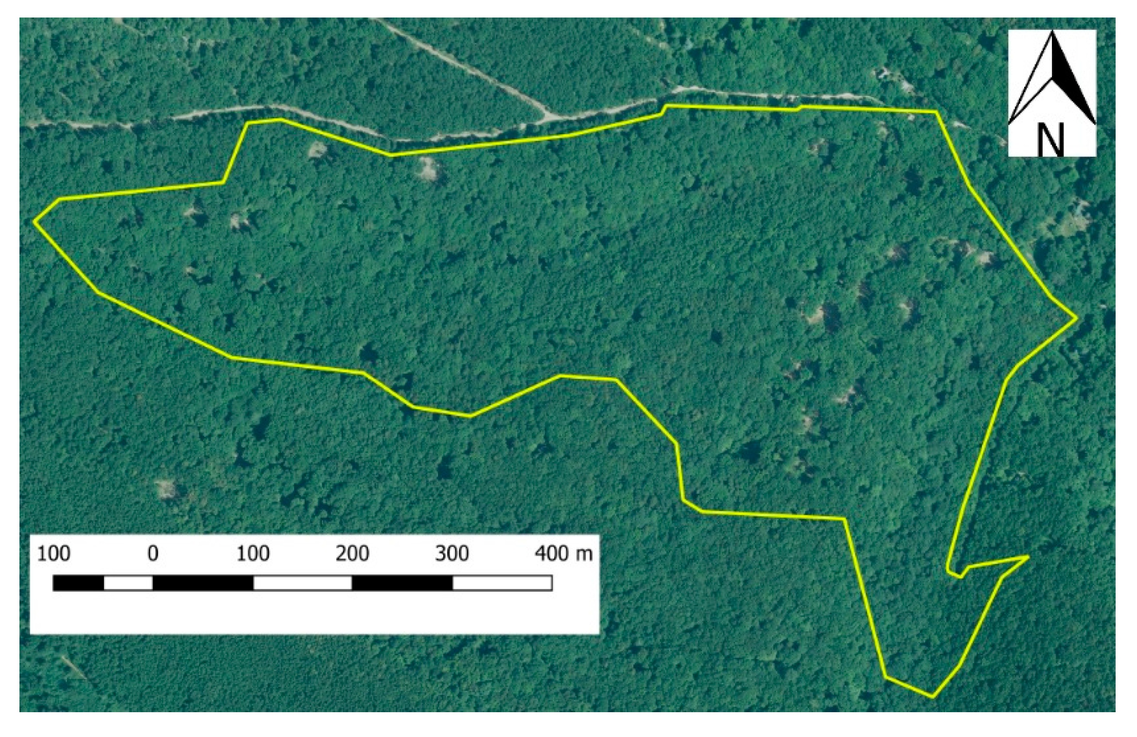
The forest compartments we investigated are close to Kismaros village (47°50′43.20″ N 18°58′37.57″ E) (Figure 2). The total area of the site is 28.4 ha. Hillsides with different aspects, small mountain ridge and a small valley compose the topography of the study site. The mean height above the sea level is 160 m. It is dominated by Oak (Quercus petraea L.) and Hornbeam (Carpinus betulus L.) with some beech forest patches. At the bottom of the gap, dense vegetation is found. It consists of young tree seedlings, blackberry (Rubus fruticosus L.), deadly nightshade (Atropa belladonna L.), sedges, fern and various grasses. The first artificial treefall gaps were opened around 2007. In the winter of 2015–2016 new gaps were opened. The average diameter of the circular-shaped gaps is between 20–25 m. In most of them a seed-tree [36] was left after treefall. The role of these individually standing trees is to plant the gap with seeds. However, the literature says gap is defined only when the mean height of trees in the gap is under 2 m [11]. In that case we would have a ring-shaped gap. Since we aimed to use high resolution satellite imagery, detection of individual seed-trees is limited by the spatial resolution of a pixel. We consider each of these gaps as a compact-shaped [37] object to simplify the methodology. The canopy closure is naturally high outside of the gaps within this climatic region. Of course, there are plenty of minor natural gaps in the canopy layer. Some trees have less leaves than others based on their health and position, and abundance of nutrition in soil [38]. There are some natural gaps in the small valley. Due to the high erosion under the roots these trees fell down naturally. Now they are coarse woody debris (CWD), which is an important source of biodiversity [39]. Thanks to the diverse topographic formations and forest types occurring in this relatively small area, we can test our assumption here because different lighting conditions are present.
2.1.2. Oak Study Site II. (OS2)
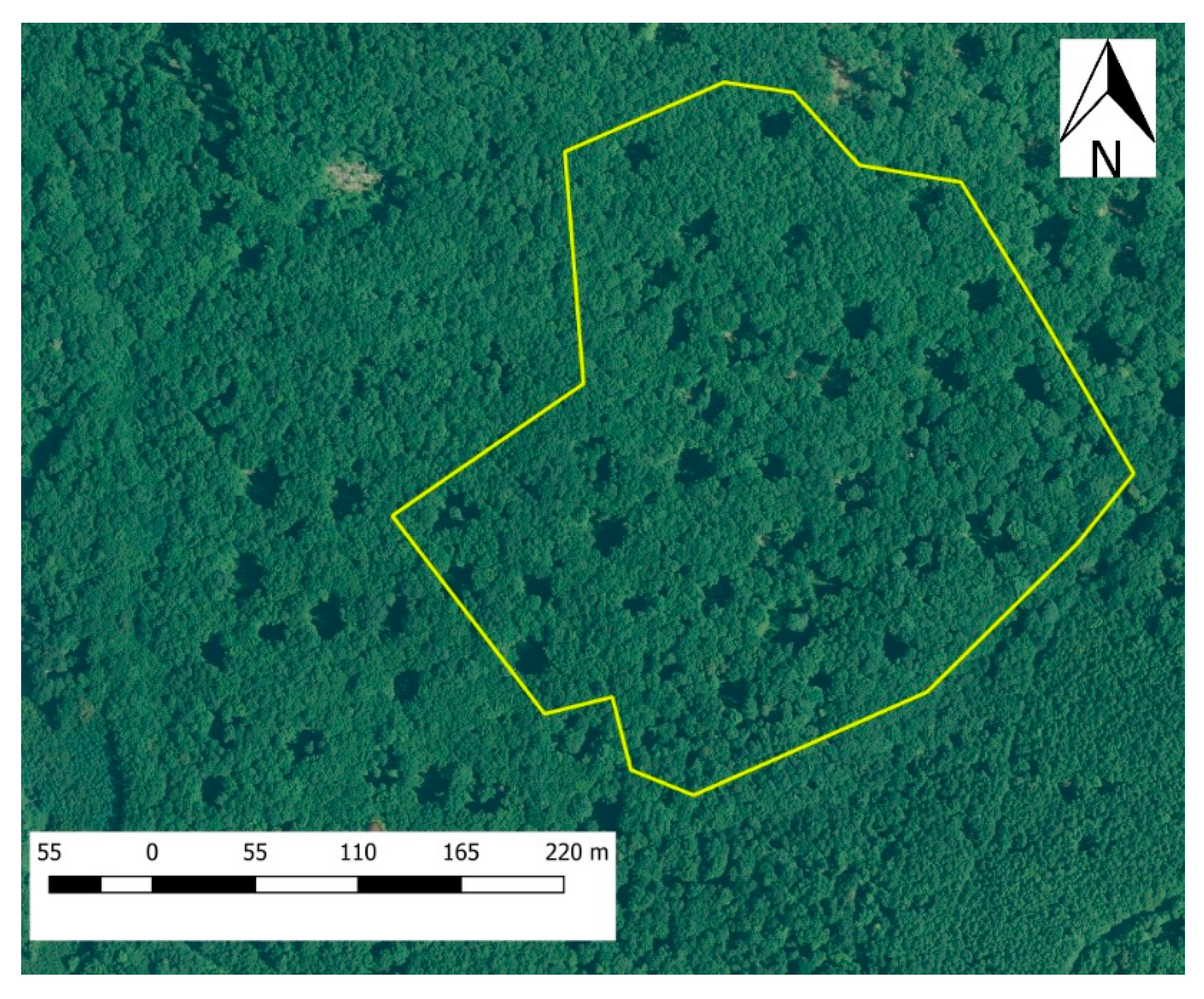
The other oak-dominated study site (47°53′11.60″ N 18°56′33.40″ E) is situated close to Kóspallag village inside the Börzsöny Mountains (Figure 3). It is dominated by the Hornbeam-oak forests as OS1. The mean height above the sea level is 370 m. The total area of the site is 8.88 ha. It has a homogenic, slight western topographic exposure. Therefore, many fewer topographic shades are present at lower sun elevation compared to OS1. The mean height of the forest is 25 m. Artificial gaps have been present since the 2000s. Between 2015 and 2016 there was no change of the treefall gaps. Their shape and dimension is similar to the gaps on the other oak type site. Since most of the gaps are more than 10 years old, the canopy started to overgrow the gaps. Thus, the original size has been reduced and sometimes it is barely recognizable even on VHR aerial images. The canopy closure can be considered as 100% outside the gaps. There are various aerial VHR images available for this site to create models for validation.
2.1.3. Beech Study Site (BS)
The 38.2 ha beech-dominated study site is situated in the higher region of the mountains (47°55′55.78″ N 18°56′37.61″ E) (Figure 4). Its mean height above sea level is 750 m. The dominant tree species is beech. Additional tree species with a lower mixture ratio are present: sessile oak, ash (Fraxinus excelsior L.) and sycamore maple (Acer pseudoplatanus L.). The exposure of this site is southwestern. The mean slope angle is 20°. The more homogeneous topography is compensated by a heterogenic vertical forest structure. Several natural disturbances since the late 1990’s have affected the structure of this beech forest at the study site. These events and the usage of artificial treefall gaps transformed the even-aged forest into an uneven-aged forest. Studies were carried out for modelling the natural disturbances [31,35] including this study site. The site was affected by ice damage in 1996, 2001, 2004 and 2014 and by wind fall in 1999 and 2010 [40]. The recent ice damage caused mainly broken crowns and less treefall because unstable trees had already fallen due to the previous disturbances. Due the fast and strong natural regeneration of beech [41] in the treefall gaps, the terrain is covered by seedlings and young trees and some weeds [42]. The mean height of the old trees is 26 m. The heights of the young forest inside the tree fall gaps vary according to their age but they are clearly separating from the older forest parts. The shapes of gaps differ from the oak type. Their diameters are much larger (30–40 m) and the shape is less compact. Often, adjacent gaps are connected into bigger patches.
2.2. Aerial Data
A digital surface model and orthophoto from the late summer of 2015 were available for the whole Börzsöny Mountains. It was made from 0.2 m ground resolution multispectral aerial images, captured with a Vexcel UltraCamX (Vexcel Imaging GmbH, Graz, Austria). Improved exterior orientations were provided by the forestry company who owns the dataset. Further Global Navigation Satellite System (GNSS) ground control points (GCPs) were measured with a Leica 1200 GPS system. The processing was done with Trimble Inpho® software (version 7.0, Trimble Inc., Sunnyvale, CA, USA) using the existing exterior orientations and the GCPs. The DSM (Digital Surface Model) was generated using the Match-T module [43]. The dense matching was carried out on a 0.5 m resolution grid using an extreme terrain type option. A DSM with 0.5 m and 2.0 m grid resolutions were created from the point cloud using Inpho (version 7.0, Trimble Imaging-Stuttgart, Stuttgart, Germany). An orthophoto was created for the study area using the DSM. The gaps which were opened before 2015 are usually visible. The matching algorithm cannot match the shadowed pixels inside small canopy gaps on the image pairs. This happens when there is a low texture present on the images like shadowed areas [44]. In that case, there is no valid automatic height measurement at the bottom of the gap. Thus the interpolated surface will not go down to the terrain and the gap is filled on the model. The surface of the canopy layer is rough where each part of the tree crown projects shadows to another part or to another tree. This can also cause uncertainties because it looks identical to smaller treefall gaps on the image. For the OS1, a commercial orthophoto from summer 2016 is available with a 1.0 m spatial resolution [45]. On the BS, no major change with the treefall gaps area is assumed between 2015 and 2016. Therefore, the orthophoto from 2015 could be used for validation of Sentinel-2 images from 2016 on that site. An aerial laser scanning (ALS) dataset was available for a small part of the Börzsöny Mountains which covers the OS2. The dataset was recorded with a LEICA ALS-70HP system (Leica Geosystems AG, Heerbrugg, Switzerland) on the morning of 29 August 2015. Simultaneously, aerial images were captured with a LEICA RCD 30 RGBN 60 MP type camera (Leica Geosystems AG, Heerbrugg, Switzerland) with a 0.1 m ground resolution. The dataset consists of 3 flight strips. The average point cloud density is 27 points/m2. The preprocessed point cloud and the orthophoto were provided by the Ipoly Erdő Zrt. It covers several forest compartments where artificial treefall gaps are being used to transform the forest structure. The topography under the forest is not as diverse as at the OS1 and therefore, only one illumination class is present. The ALS dataset was used during the spectral treefall gap modelling.
2.3. Satellite Images
Generally, 11 Sentinel-2A images were used in the research (Table 1). From the R036 and R079 satellite footprints, the 33UYP and the 34UCU granules 100 × 100 km (Figure 1) [24] were used with their original map projection. There is about a 180-degree difference in the azimuth viewing angle of the sensor above the study area on the two granules. The sensor viewing zeniths are similar owing to the sensor’s detector array design [24]. Due to the bidirectional reflectance distribution function (BRDF) effect on Sentinel-2 [46] images, direct comparison methods on pixel values in a time series cannot be used. Sensors had a mean altitude of 786 km and the tree height was approximately 25 m so there is a minimal amount of occlusion of the view, which occurs only at a subpixel level on the gap bottom and forest pixels. We investigated the L1C, the L2A reflectance and the topographically corrected (L2ADEM) data types of Sentinel-2A. The topographic normalization was done using the SRTM [47] 90 m resolution elevation model. All the reflectance products were created with the Sen2Cor 2.3.0 software (European Space Agency, Paris, France). From 2015 there were 2 images and from 2016 there were 9 images. Not all of the images of the study area were totally free of clouds. Therefore, some of the images of individual study sites were excluded based on the cloud and cloud shadow coverage.
The first image of Sentinel-2A was acquired 4 days after its launch on 29 June 2015. [48]. The satellite became operational on 9 September 2016. [49]. Most of the analyzed images were acquired before the operational stage so there was a minor difference between the orbits. Due to the pre-operational phase of the satellite, the early images have a weaker geometrical accuracy. The precise orbit of the satellite and the exact date and time of the image acquisition is known thanks to the two GNSS instruments onboard [24]. The sun positions and sensor viewing angles are stored in a 5 × 5 km grid. This makes it possible to model the illumination of the study area.
2.4. GNSS Reference Data
We did GNSS point measurements in the treefall gaps in the winter of 2016 at the OS1. A total of 79 artificial treefall gaps were measured in the assumed center with a Trimble Juno SB handheld GNSS instrument. This dataset was used for validation along with the aerial reference datasets. Since the area could be determined more precisely from aerial data than with field measurements, we did not measure the area with GNSS.
3. Methods
A complex workflow was developed for detecting treefall gaps (Figure 5). It consists of a shadow modelling, spectral unmixing and image mosaicking steps. A synthetic treefall gap method was used for the area evaluation.
3.1. Shadow Modelling
Topographic normalization is the common method to eliminate differences caused by shadowing [50]. This method balances the reflectance values according to the position of the shadows on the surface. There are several methods [51] to perform the normalization. The most common methods use only terrain-dependent, terrain- and wavelength-dependent [52] or terrain- and reflectance-type dependent methods [50]. Their result can be used with confidence on a regional scale. In our case it would generate more uncertainty on a local scale if some of the parameters like an inaccurate elevation model are included during the correction [51]. Therefore, we could not always rely highly on a topographic normalization.
The differently illuminated areas were delineated and handled according to the condition of the illumination. The shadows for a scene were modelled on the 2 m grid resolution digital surface model (DSM). We modelled the shadows on the topography with the widely used “hill shade”, that creates a shadow layer which is perceptible to the human eye [53]. While the projected shadow calculation is a global function on a raster, the shade calculation is focal. To calculate this requires the slope and the aspect of the elevation model and the sun position. If we use a 3 × 3 window for the focal function, it means calculating only a 6 × 6 m window with a 2 m resolution model. The result would be too fine for a 10 m resolution image to compare. For this purpose we resampled the surface model to 10, 20 and 50 m resolution by averaging. The relative solar incidence angle, or illumination condition (IC) [52] model was generated at all resolutions. The pixel values range from −1.0 (totally shadowed) to 1.0 (totally illuminated). The sun azimuth and zenith angles were derived from the Sentinel-2 product for the study area. The illumination model was generated on 19,255 ha covering a part of the Börzsöny Mountains, and is expressed in the following equation:
where Z = Solar zenith angle (rad), S = Topographic slope angle (rad), ϕZ = Solar azimuth angle (rad), and ϕS = Topographic aspect angle (rad).
With a K-means function [54], the different illumination conditions were clustered into 3 classes using a moving averages of classes method. The benefits of this choice will become visible in Section 4.1. We decided to use the 3 classes, based on a visual examination of the images. The illuminated, neutral and the shadowed classes were created. The range of the illumination values depends on topography and sun position. The cluster means from the 50 m resolution illumination were used for thresholding classification of the 10 m resolution illumination pixels. The 10 m resolution illumination map based on the DSM contains more pits, which are homogenized by the 20 and 50 m resolution. Therefore, the 20 and 50 m illumination maps show a continuous surface.
3.2. Spectral Unmixing
The mean height of the forests is around 25 m at all study sites. The diameter of a gap is approximately 20 m. When the satellite passes the study area in the morning (9:50 GMT), a projected shadow is visible on the bottom of the gap if it has neutral or northern aspect. This causes significantly lower NIR values in the gap among with the other bands. The ratio-based indexes like vegetation indexes [55] would normalize this difference. The gaps in the southern aspect have just the opposite spectral profile. Direct sunlight reaches the bottom and young trees or dense vegetation show higher NIR values than the neighboring trees. This phenomenon occurs especially in beech forests where the gap is usually bigger than for oak forests.
Using spectral mixture analysis, the pixel spectrum can be decomposed into a collection of constituent spectra which are captured under the pixel spatial distribution [56]. The abundance of the feature fraction inside the pixel is transformed into fuzziness when multiple spectral endmembers are used. These endmembers represent the pure spectral response of a feature. It belongs to the soft classification methods where individual pixels are assigned to more than one class with a known ratio of membership [57]. On the highest resolution bands of the satellite with 10 m, the treefall gaps (as features) occur as a mixed pixel with forest in most cases. That is why hard classification methods would not give the best results every time.
Multi-temporal, spectral unmixing has been used in some cases with success [58,59]. The multitemporal spectral library of endmembers can increase the accuracy of the unmixed results [60]. In that case, the layered stack of images from different date are co-registered and the whole stack is used for the unmixing process. Landsat TM data is also suitable to detect change using spectral mixture analysis [61]. Due to the high resolution and the slightly different view angles and sun positions, an indirect multitemporal spectral unmixing was carried out. The individual images were unmixed and only these results were analyzed as a multitemporal dataset.
The linear spectral unmixing method was chosen with multiple endmembers for processing individual Sentinel-2 images. This model assumes that the spectra of pixels consists of the linear combination and the residual errors of the subspectras of the landcover types. They separate clearly when we study the spectral profile of a forest, a gap and a young forest. Typically, spectral unmixing is used with hyperspectral imagery [62]. It uses n linear equations per pixel where n is the number of bands used on the image. The unknown in the equation is the abundance of the material. It is important to have fewer unknown parameters than equations. We used fewer endmembers than the number of bands. In total, 4 bands were available from the multispectral image and 2–3 endmembers were used as a spectral sample from each forest type from each illumination class. This relationship is expressed in the following equations:
where Rk—Reflectance of source at wavelength k, Ek,i—Reflectance of endmember I at wavelength k, ai—Abundance of endmember I, εk—Noise from the sensor and modelling error at wavelength k, RMSE—Root mean square error of the εk, n—Number of endmembers, m—Number of wavelengths in the discrete spectrum.
The linear spectral unmixing was carried out by a least squared method [56]. The fully constrained solution guarantees that the sum of the endmembers inside the pixel has a maximum of 1.0 and it is non-negative. It uses the non-negative least squares method (NNLS) which was solved with an iterative solution. This algorithm is found in various commercial and open source remote sensing softwares. We used the Fully Constrained Linear Spectral Unmixing algorithm [63] from the BEAM toolbox which was developed specially to support ESA’s Earth Observing missions. It is available with a GNU license [64].
In the oak forest study sites, 2 endmembers were used for each illumination category:
- Forest feature
- Shadowed treefall gap feature
In beech forest study sites, 3 endmembers were used for each illumination category:
- Forest feature
- Shadowed treefall gap feature
- Fully illuminated young forest feature
3.3. Endmember Creation
The spectral unmixing was implemented for each Sentinel-2 image. The endmembers were derived from the actual image automatically on each date. Therefore, individual pixel positions were collected by visual interpretation from satellite images which were assumed to be a non-mixed pixel. The sampling positions were selected on a cloudless image from 28 August 2016. The selected pixel positions were stored as geographical coordinates. The spectral samples were collected from these locations. With the recent calibration of Sentinel-2A, 10 m bands do not have a huge dynamic over slightly different aged and mixed deciduous forests. Using the 20 m bands, [25] it is possible to differentiate the forest types but it is not our purpose in this research. Assuming the lower dynamic, the same spectral sample can be used everywhere in the region. Three classes were determined for the beech forests: old forest, young forest, and shadowed treefall gap, and two classes for the oak forests: old forest, and shadowed treefall gap. The sampling positions covered the whole Börzsöny Mountains. The type of the forest was determined by using a forest management inventory because it is hard to classify them visually on a Sentinel-2 image. A cloud mask was used during the sampling to avoid clouds and cloud shadows. This mask was generated during the preprocessing of L2A type images [65]. Further filtering was done according to the blue band (B2). This method is based on the LandtrendR [66] software where it was used for manual correction of cloud masks. Kennedy et al. used the Landsat TM Band 1 which covers the same spectrum as Sentinel-2’s blue band. The fixed threshold for reflectance at B2 was determined at a pixel value 1000 based on the histogram of the images.
The endmembers were created from those sample pixels where illumination classification was available for their positions. The samples were reclassified based on their illumination. The classifying thresholds were taken from averages of 50 m resolution clusters. Therefore, the 10 m resolution illumination map and the Sentinel-2 image were merged to carry out the data collection. Using the illumination class, the forest type and the feature type, the samples were grouped into the classes of young forest, forest and shadowed treefall gap. The mean and the standard deviation (SE) were calculated for each group. The mean of the image bands was used as an endmember. The SE of the group was used as a quality marker.
3.4. Mosaicking Unmixed Images
After the spectral unmixing, there are 6 unmixed images present for each Sentinel-2 image. Two unmixed results belong to each illumination category. There was one oak forest with two features and one beech forest with three features. Prior knowledge of the forest type for the site was used, which reduced the number of unmixed results to the 3 illumination categories. These 3 images were mosaiced together based on the previously created 20 m resolution illumination map, which modelled the actual sun illumination classes on a DSM. Since the young forest, and the shadowed gap features cover the treefall gap in a beech forest, we applied a union for them. After their combination, only the forest and the treefall gap feature remained for both forest types. The ratio of the illuminated young forest and the shadowed young forest depended on the position of the sun which varies from scene to scene during the year. Thus, there was no reason to keep them as different types. The resulting mosaiced image contained 3 bands:
- Band 1: Forest abundance
- Band 2: Treefall gap abundance
- Band 3: Illumination category
The sum of Band 1 and Band 2 on the mosaiced image must be 1.0 according to the used spectral unmixing method. The amount of treefall gaps were used for the further processes which represented their fraction inside the pixel.
3.5. Synthetic Treefall Gap Modelling
A workflow for synthetic treefall gap modelling was created (Figure 6). The aim of this method is to create a spectral mixture model for the treefall gap which can be seen from the Sentinel-2. From this model the threshold value for filtering the treefall gap fraction in a pixel was estimated for each Sentinel-2 image and the synthetic gap was modelled using the created endmembers.
An ALS-based normalized digital surface model (nDSM) was used for this purpose. The DSM was created by using the DSM module [67] of the OPALS software [68]. The surface models were created with a 0.5 m resolution. This DSM is a combination of a maximum surface and a moving least square interpolation which shows less artificial roughness and smoothing. Thus, it better represents the break lines like the edge of the treefall gaps. The digital terrain model (DTM) was generated with the SCOP++ software (version 5.5.0, Trimble Imaging-Stuttgart, Stuttgart, Germany) using the hierarchical robust interpolation [69,70]. The nDSM was created by subtracting the DTM from the DSM.
Six gaps were selected from a naturally illuminated site from the DSM. Three gaps contained a seed-tree inside and three had no seed-tree inside. The reference gap mask was created by using a 2 m vertical threshold for the nDSM. The sun positions were used to model a projected shadow on the surface by view shed analysis. At this point we calculated the fraction of the shadowed area and the illuminated area inside the gap. Also at the VHR nDSM, the roughness of the canopy surface became visible after the shadow modelling. Since the spectral signature of a shadowed canopy part and the shadowed gap is similar, it is important to know how different sun positions change the amount of shadows. The three spectral signatures were created from the endmembers. These spectra were assigned to the 0.5 m resolution pixel according to the mask and the shadow model. If the mask pixel was a canopy, it produced forest signature or gap shadow signature spectra. If it was inside the gap mask, it produced gap shadow or illuminated young forest signature spectra. The 0.5 m resolution image with its 4 bands was resampled to the 10 m resolution by averaging. This makes an image which looks like a real Sentinel-2 image. The same spectral unmixing method was applied here which was used for the main workflow. The endmembers for the unmixing were the same which were used for spectral mixing. Reference pixels were chosen at the 10 m resolution using the gap mask, which visually represents the treefall gap. For these pixels the gap fraction values were used as a thresholding minimum in the main workflow. This was done for each illumination class.
This method is also useful for estimating the ratio of the detected area and the reference area. It is assumed that the detected area on the satellite image highly depends on the elevation of the sun. The L2ADEM type data endmembers were used for the modelling.
3.6. Area Evaluation
3.6.1. Area Evaluation on Individual Images
Each unmixed and mosaiced image contained the treefall gap abundance value for each pixel. Since shadows in the canopy generate small shadowed gap signatures in the canopy layer, filtering has to be applied for the abundance values. These filtering thresholds were determined during the synthetic gap modelling. If a gap abundance value was under the threshold, it was considered as 0. The calculation of the area was based on the filtered treefall gap fraction inside the pixel and the pixel’s ground resolution. By multiplying the area covered by the Sentinel-2 10 m resolution pixel with the treefall gap fraction, the result ranged from 0 m2 to 100 m2. These pixel values inside the study site polygon were summarized, which resulted in the total area of treefall gaps. This process was carried out for each study site with all useable unmixed images.
3.6.2. Time Series Construction
Two methods were used for the evaluation of the unmixed images. With the first method only the mean value and the SE of the evaluated area was calculated. This method allowed us to get a simple comparison between the evaluated treefall gap area and their reference area. It created a comprehensive result, but it neglected the spatial distribution of the treefall gaps. The number of correctly detected treefall gaps therefore cannot be defined, because the reference has a different data type. The spatial correlation of the transformed reference showed the goodness of the fit.
This method is based on a time series construction. A 10 m resolution grid was placed over the study site in the national projection system (HD72/EOV, EPSG:23700). The nearest pixel from an unmixed result was assigned for each grid centroid and their values were stored as an attribute. Since the unmixed images were still in a UTM projection, a coordinate transformation [71] was applied in this step. After assigning all individual images to the grid, a GIS vector layer was available for the analysis. It contained a treefall gap fraction value for each grid cell which went through an individual noise filtering. The treefall gap fraction ranged from 0 to 1 on each individual date. That allowed us to turn their value into probability. Their values were summarized and normalized for each year. We suspected that no significant change took place during the vegetation period during a year. The normalized value on the grid showed the fuzziness of the detected gaps. If it had a value 1.0, it appeared on every date as a treefall gap. If the fuzziness was lower, it could be a part of treefall gap or a false detection. If a false detection was caused by the shadow of low sun elevation, it appeared only a few times. If the number of observations are sufficient, with an observation from each month during the vegetation period, the fuzziness value over these false detected cells will be much lower than if it would cover only a small fraction of a real treefall gap. Therefore, a global filtering was applied for the normalized treefall gap fuzziness value. This global threshold was estimated empirically based on the results. The threshold value was not used in the area evaluation. We detected changes by comparing the fuzziness values from different years. This also created a change map.
The nearest-neighbor sampling method could cause a subpixel shift on the results. According to the preliminary tests, it was always less than 3 m.
3.7. Spectral Sample Subsampling
We wanted to determine the optimal number of spectral samples to create endmembers. Therefore, a subsampling was carried out using the existing endmember samples. We subsampled the spectral sample dataset from 100% to 10% by 10% steps, and from 10% to 0% by 1% steps. The subsampling was done by random selection. An array containing the indexes of the spectral samples was randomly shuffled by C++ STL function [72] and the first n element was selected to create an endmember, where n is the number of samples at a certain subsampling ratio. When the subsampling ratio was set to 0%, it used only 1 randomly selected sample. The endmembers were created from the subsampled spectral data for the forest and gap features. The unmixing workflow was done using the created endmembers for each Sentinel-2 image. Two hundred iterations were done for each Sentinel-2 product (L1C, L2A, L2ADEM). Each treefall gap fraction area was evaluated from the unmixed results. A constant 0.7 threshold was applied for each image. The mean value of the area from iterations was considered during the evaluation.
3.8. Validation
The reference treefall gap maps were created from the aerial photos, orthophotos and the available DSMs. The treefall gap polygons were created using multi-source visual interpretation. The polygons were drawn on the orthophoto. The DSM and the stereo pairs of aerial photos were used for reducing uncertainties. Only the visible parts of the gap were drawn. The seed trees inside the gaps were excluded from the polygons. The polygon vertexes were dropped with approximately 0.5 m accuracy over the edges of the treefall gaps. The GNSS measurements from the OS1 were used to separate artificial and natural gaps in the canopy. The spatial validation of the map with the reference treefall gap polygons was done on the grid polygons. The GIS vector layer of polygons was merged with the 10 m resolution grid polygons. After this operation, the remaining fraction of a treefall gaps was assigned to the grid which already contained the remote sensed gap fraction. A correlation was calculated between the remote sensed and the reference data values.
4. Results and Discussion
The main aim of this research was to determine the area which is covered by treefall gaps and to create maps from them. We carried out the method on a satellite image time series. Three types of satellite imagery were used: L1C, L2A and L2ADEM datasets. Our assumption was that the different types of preprocessing highly influence the results. In the oak forests, 9 images, and on the beech forests 6 images were evaluated due to cloud cover restrictions on the further images. The rest of the images were used only for spectral sampling.
4.1. Endmember Evaluation
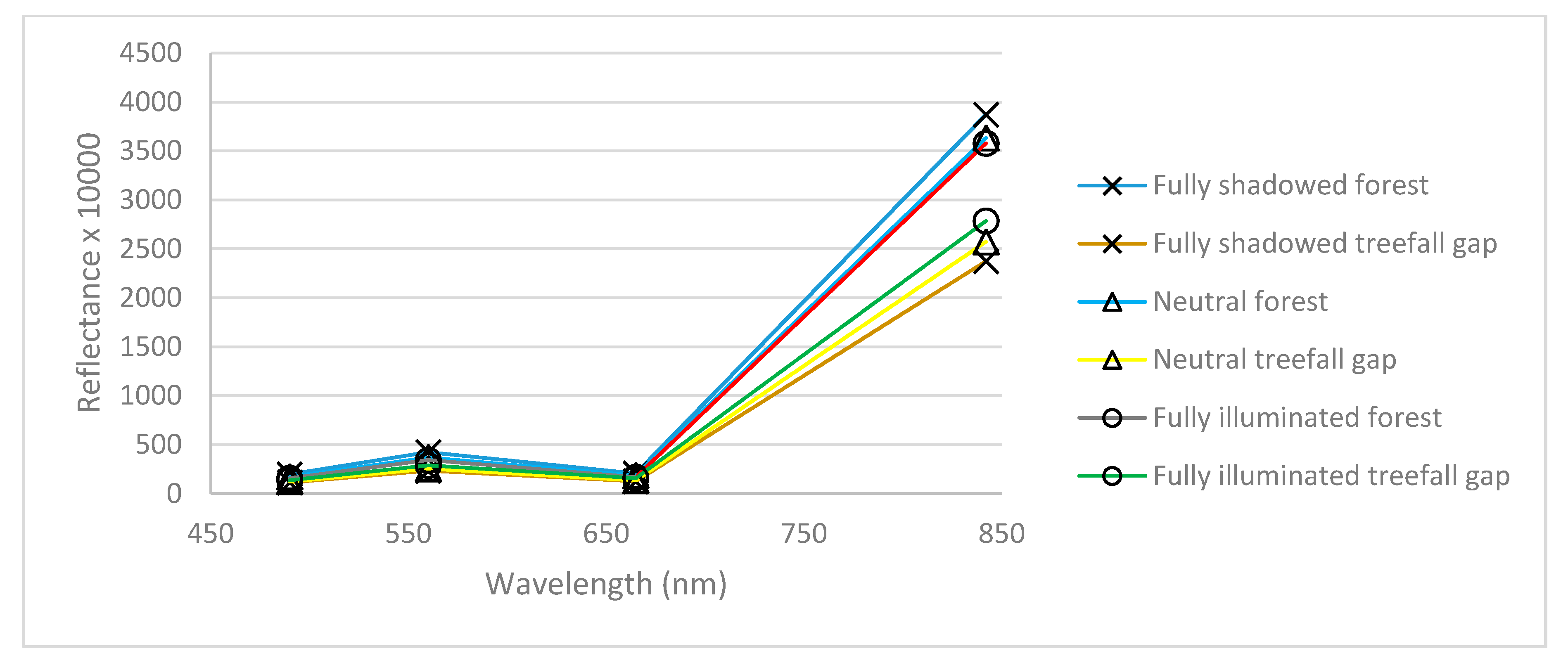
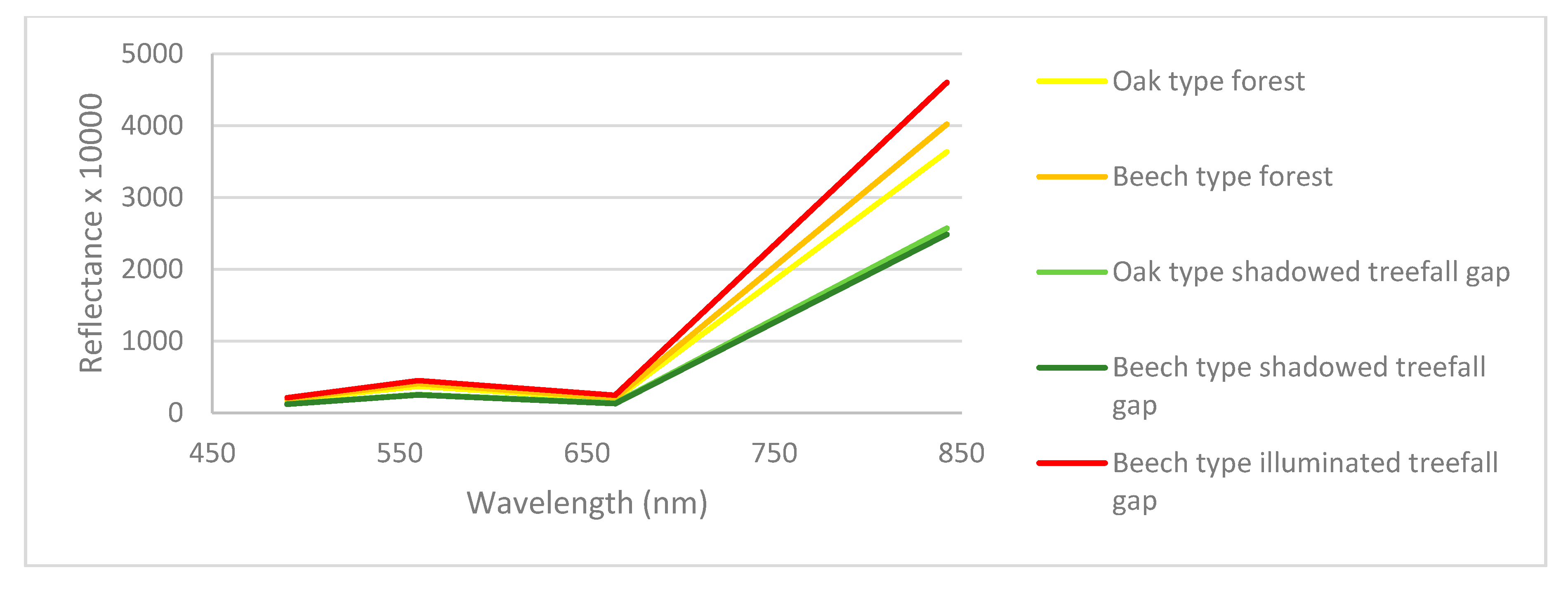
It was visible that the endmembers would have too much variation if the range would be not split into 3 illumination classes as shown in Figure 7. The feature types in the created classes are located separately in the spectral space (Figure 8). Since we were looking at vegetation the NIR spectrum has a main response to the features. But other bands also show differences in their spectral profiles. Spectral features with oak forests always show higher NIR values than the gap features due to projected shadows inside the gap. The forest endmembers in a lower illumination class overlap with a gap endmember from a higher class. This result proves that the spectral mixture analysis should work with better accuracy if illumination is considered.
The mean and SE of the endmembers showed a prior accuracy of the spectral unmixing. A SE value bigger than 1000 on the NIR band indicates an unreliable result. The SE at the NIR band on cloudless images ranges between 0 and 1000. On images with partial cloud cover, due to the errors of the cloud mask, the SE was much higher. After applying a threshold filter on B2, the SE was reduced on each band. Results from the L1C data, where only geometrical correction was applied, showed the lowest SE with 166 on the NIR band on all endmembers, while L2A products had 210 and L2ADEM 251.
The sample positions for the endmembers cover almost the whole Börzsöny Mountains so they come from different altitudes. Even an 800 m height difference occurred between sample positions inside the same class where there is a difference between the aerosol and water vapor thickness (Table 2). The proportion of the useable sampling positions on individual images was calculated (Table 3).
We would expect the lowest SE for endmembers with the L2A radiometrically corrected imagery. In the L2A radiometrically and topographically normalized data type, the SE of the endmembers was higher as expected. The reason for this is the inaccurate DEM (SRTM 90) or the topographic normalization method [73] which caused over-correction of spectral values. The correlation of the endmembers from different data types (Table 4) showed that the atmospheric correction is highly dependent on wavelengths. Aerosols in the atmosphere affect the blue band (B2) most while the topographic correction made only minor changes according to their correlation. This phenomenon was also observed on the green band (B3). The radiometric correction showed less change over the NIR range, and the difference at the correlation is much smaller but it did change the values. In the beech area, the Spectral profiles of young and the old forests converge while without topographic normalization they were clearly separated. In oak forests the distances between the spectral profiles stayed constant where only old forest and shadowed treefall gap features were present.
4.2. Subsample Number of Endmember Samples
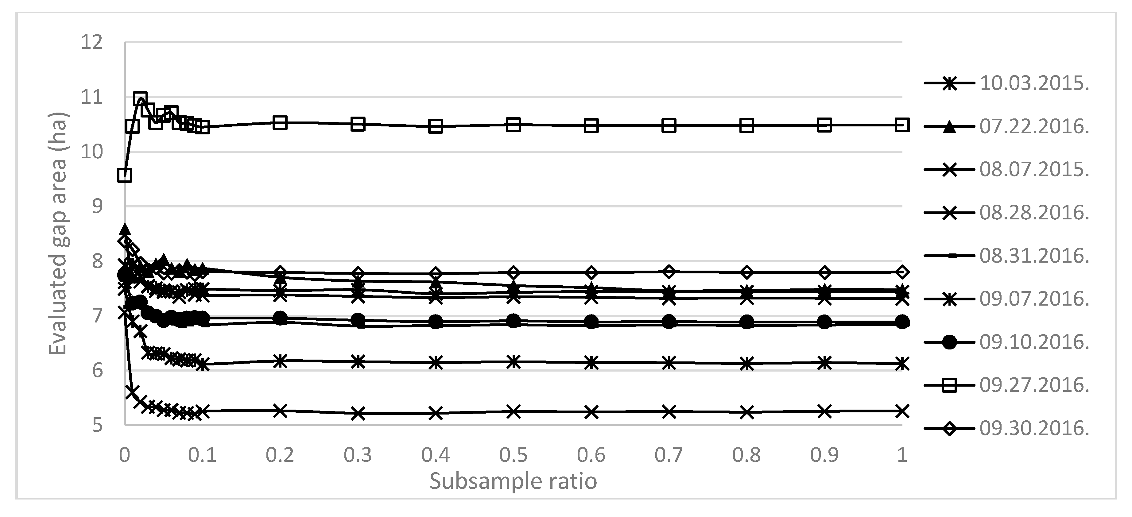
We tested the effect of decreasing the number of samples during the creation of endmembers (Figure 9). According to the area evaluation on the subsampled results, there is only a minor difference above the 10% subsampling ratio. In certain cases only 1 really good endmember for a feature type was enough for each date. This could not be guaranteed so numerous samples are still required, which forms a normal distribution.
Increasing the number of samples for creating endmembers increases the accuracy of the mapped treefall gap positions by the law of large numbers. The optimal number of samples based on this test would be 100–200 rather than a few thousand as we had.
4.3. Synthetic Treefall Gap Modelling
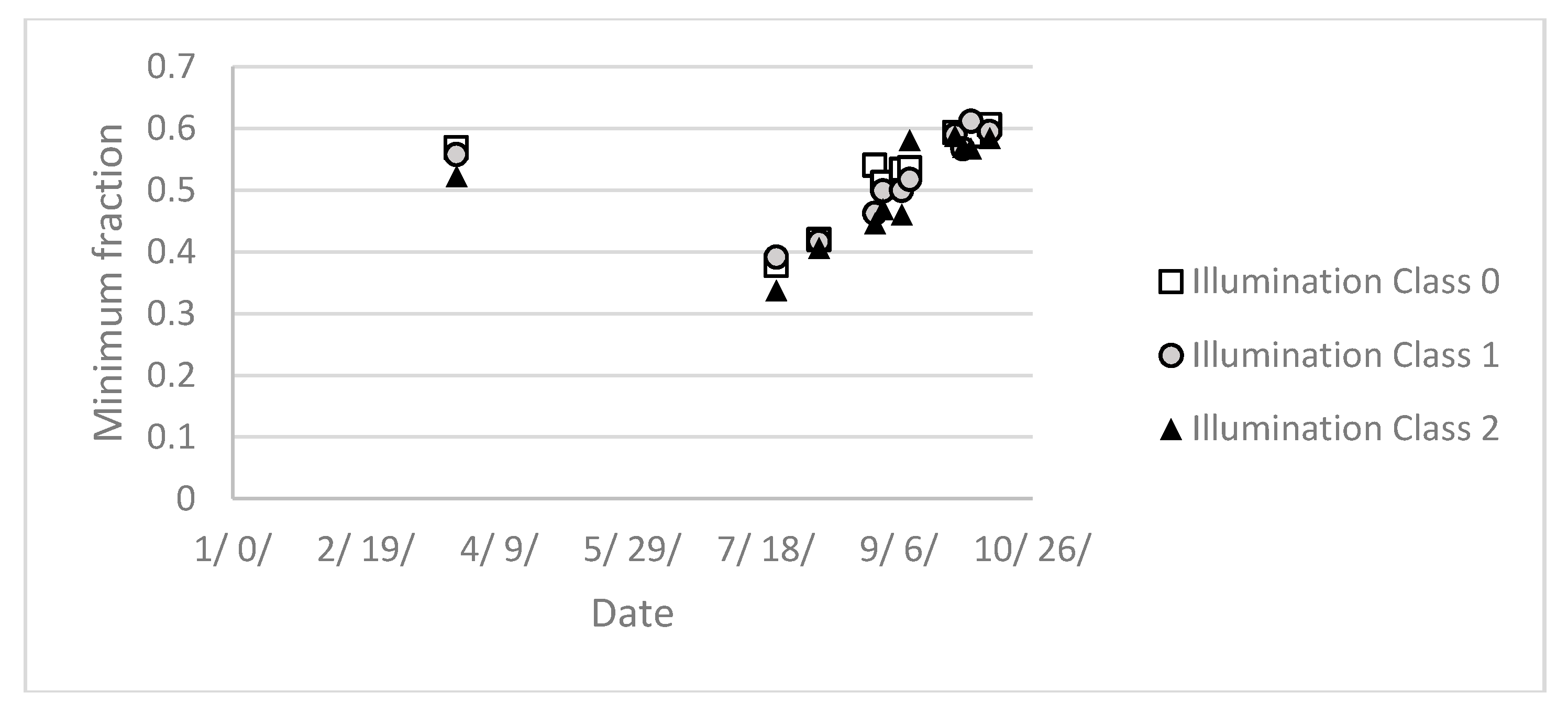
The spectral mixing and then the unmixing was carried out for the selected 6 treefall gap models. All 11 available images were used for the modelling. The minimum fraction on a treefall gap in the visually selected sampling pixels showed the expected pattern through the year. The correlation between the minimum fraction and the elevation of the sun is −0.98. It indicates that the detected amount of shadow which we handle as a treefall gap highly depends on the elevation of the sun. The lower the sun’s elevation is, the more false detections take place. Therefore, a dynamic thresholding value is required for area evaluation on each date. For thresholding, the minimum fraction value was used (Figure 10), which is the average of the minimum fraction of all sampled values.
The evaluated area on the selected sampling pixels was inspected. Using the threshold values, which were calculated previously, the overestimation of the spectral unmixing was modelled. It showed that on average the time series will display the exact area (Figure 11), but individual images could have bigger overestimations in relation with the angle of elevation of the sun.
4.4. Gap Area Evaluation
4.4.1. Oak Study Site I
From the aerial orthophotos in the year 2015, 1.79 ha were evaluated as a gap area. From the aerial orthophotos in the year 2016, 3.29 ha were evaluated as a gap area. The change was 1.50 ha. This area is including the canopy of the single seed-trees inside the gaps. The results exclude those trees, because the satellite imagery is limited to its 10 m resolution.
The natural canopy gaps over the small valley which divided the site into two parts were masked. The image dynamic in that area over the year was so low that valid gap detection was not expected there. The area for evaluation was reduced to 26.3 ha. The area for the treefall gaps was calculated on each single image. Two images from 2015 and seven images from 2016 were evaluated. The individual filtering for each date was applied based on the synthetic treefall gap modelling. Basic statistics were calculated for each year and for each data type (Table 5).
According to the results, the L2A radiometrically and topographically corrected imagery showed the most reliable results for this area. The simple L2A results showed a double amount of gaps with a bit less SE. Despite that the L2A DEM endmembers had a higher SE, the result is surprisingly good on this type of forest both spatially and quantitatively. The change from 2015 to 2016 showed different results. There was almost 1 ha difference, which is 3.5% of the total area, when comparing the biggest to the smallest data. The gaps appeared where reference points were measured on the field but their size was larger than the reference. The georeferencing quality test on some images failed the quality test during the preprocessing of L1C products according to the metadata. The different view angles of the sensor caused a subpixel shift in the result. Some treefall gaps were situated on the border of the study site right next to a road. The sub-pixel movement in the georeferenced areas caused some errors there with the automated evaluation.
There is no regular error between the images which were taken from different orbits. The evaluated area of gaps depends more on the vegetation phase and the lighting conditions. The two types of L2A-based maps showed better overlapping. The L2A DEM maps have more transparent outlines around the gap center. We observed that the adjoining gaps sometimes appear to be fully joined, but on other dates they look separate. This is because their thin border of canopy sometimes mixes into the gap, or sometimes appears individually based on amount of self-shadowing. The different view angles of the sensors could also influence a result with a few pixels’ difference. This was also inspected by view shed test.
The unmixed results from different data types were compared by correlating them (Table 6). This showed a very high correlation between the L1C and L2A images. However, the filtered results showed a much greater difference than the unfiltered results. The atmospheric correction leads to higher contrast between forest and treefall gaps, which causes the differences in area evaluation. The topographic normalization highly affects the correlation value, which makes the area evaluation better.
4.4.2. Oak Study Site II
Treefall gaps were digitalized using the orthophotos and the nDSM on a 1.24 ha area. This site was located in the middle of a forest compartment so it was free from the border effect noise. Two images from 2015 and 7 images from 2016 were evaluated. Since there were no significant changes between the two years’ treefall gap area the results are comparable. In 2015 the first image was taken in the middle of a summer at a high sun elevation. The second image was taken in late autumn. According to the spectral modelling, the average of these two dates should give a reliable estimation for the area. On the L2ADEM product it showed a really close value to the reference with a high SE. In 2016 the images were taken in the second half of the vegetation period. Thus, it brings the average closer to the overestimation which took place at a lower sun elevation.
Since this site was a flat area with neutral topographic exposure, the topographic normalization should not affect the result. However, there is a significant difference between the evaluated areas (Table 7). The correlation between the unmixed unfiltered results showed a better connection than at OS1 due to the smoother topography (Table 8).
4.4.3. Beech Study Site
On the 10 m resolution Sentinel-2 images, only the standing old forest and the young forest and gap categories could be evaluated. These two categories were used during the creation of the reference data set. The total area of the site was 32.76 ha and the gaps covered 14.11 ha according to the orthophoto from the summer of 2015. The convex hull of the crown was considered as a projection where only partial crown damage was detected on the aerial image. Two images from 2015 and 4 images from 2016 were evaluated (Table 9). This site is located in the higher region of the mountains where cloud cover is more frequent.
The previous endmember evaluation showed that the topographic normalization of the L2A data minimizes the spectral distance between the old forest and the young forest signatures. Due to this artifact, many old forest pixels were classified as a young forest which belongs to the treefall gap category. The difference between the L1C and the L2A data results are negligible. The beech sampling positions were situated in the higher region of the mountains, where the amounts of atmospheric aerosol are similar.
Furthermore, the topography under the forest was smoother but steep. The illumination of the site was more balanced. The L2A data showed the lowest SE values in the two different years (Table 9).
On the results from 2015, the damage of the 2014 ice damage was observed. The ice damage caused a partial crown loss for mature beech trees. Thus, more self-shadowing appeared where the general canopy closure was lower. This produces different textures on the orthophotos as well. On images from 2016, the gap area reduced by 22.36% and the SEs of individual results were below one hectare. This can be explained because the canopy of beech trees has a strong ability to regenerate even at older ages.
The correlation between results from different data types showed a low correlation between the topographically corrected data and the others (Table 10). This could be explained by the mixing of old and young forest spectra, which highly effects the NIR range. All the correlation coefficients are lower than in oak forests. The area results show a strong connection between the L1C and the L2A results.
4.5. Time Series Evaluation
4.5.1. Oak Study Site I
The simple area evaluation in Section 4.4 showed an overestimation on every site. Those statistics do not show any spatial distribution, and thus the type of error remains unknown. The evaluation of the time series on a regular grid gave a more accurate result (Figure 12). Turning the treefall gap abundance value into a fuzziness, produced a map for each year with information about the detected accuracy. Only the L2ADEM results were used for this type of evaluation. The area results barely differ from the simpler method in Section 4.4. The individually filtered single values constructed the final result (Table 11). A global filtering was not applied during the area evaluation for the normalized fraction value which shows the fuzziness. The correlation between the evaluated and the reference gap fractions was 0.63 for the year 2015 and it was 0.65 for the year 2016. The fuzziness map of treefall gaps overlaid to the reference data shows further details about the canopy closure. If the crown structure of a tree is looser, it appears on the map with a low fraction as a treefall gap. If the treefall gap mapping process is done on a series of images which were taken before the artificial gap opening, these noises were automatically excluded from area evaluation. The global threshold value is determined empirically at 0.25 for this effect on the summarized fuzziness map of the quantity of gaps. This value highly depends on the elevation of the sun. It was determined visually based on the thematic map (Figure 12). If more images with low sun elevation are used, this will increase the amount of false detections. The amount of false detection is negligible compared to the real gaps. Elongated gaps with low fractions in the pixel are unfortunately filtered out during the individual scene filtering. Treefall gaps with seed trees inside also cause this effect. The minimum extent that could be detected with higher confidence is a compact-shaped gap, which is not much smaller than the pixel size.
4.5.2. Oak Study Site II
The overestimation was investigated in detail on this study site, which was free from border noises and more VHR reference data were available. In total, 1.72 ha of forest were evaluated with the time series method using only individual filtering on the L2ADEM-type unmixed products (Figure 13) (Table 12). The detected pixels overlapped the reference dataset. The correlation between the reference grid and the merged time series was 0.72 without global filtering.
4.5.3. Beech Study Site
The individually filtered, unmixed L2A products were used for the time series evaluation (Table 13). The simple area evaluation in Section 4.4.3 produced acceptable results on images from 2016 (Figure 14). According to the oak study sites, the same gap border artifact should be present. The different structures of the non-compact treefall gaps and inhomogeneous tree height distribution should bring more border effect noise into the time series result. Results from 2015 showed the damaged part of the site. Tree groups which suffered partially broken crowns in 2014 can be seen on the map. The result from 2016 showed better connections to the reference gap polygons. The correlation of the merged treefall gap ratio and the fuzziness of a gap showed the value 0.21, which is significantly lower than with the oak sites since the canopy structure of a mature beech tree is much looser than a mature oak tree. This is especially so if the beech trees had ice damage several times during their lives. These effects were filtered from a longer time series. Here only the regeneration was observed. The regions where strong regeneration took place were observed on the change map of 2015–2016 (Figure 14). The differences between the reference and the calculated maps show the border effect along the edges.
4.5.4. Possible Sources of Overestimated Area
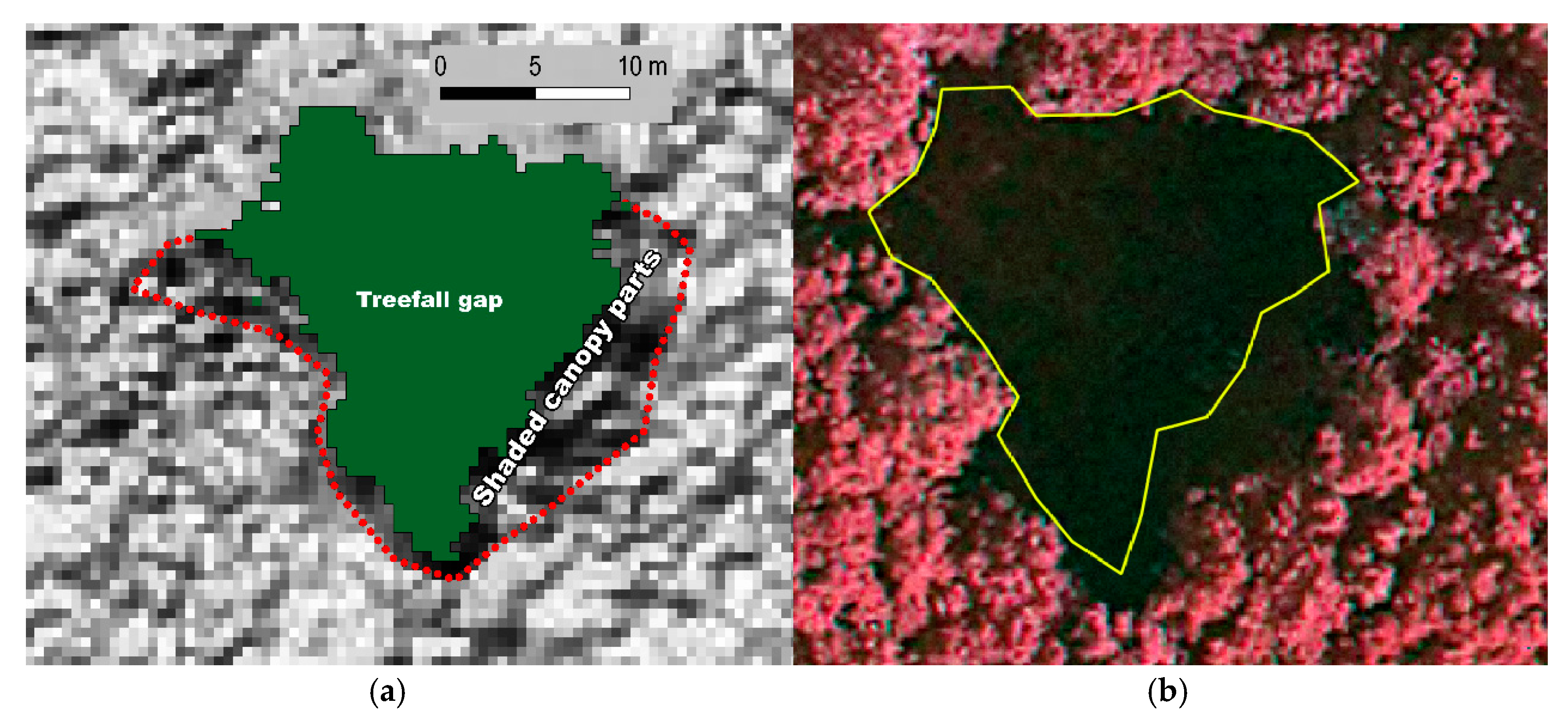
As shown on Figure 13, most errors appear around the edge of the reference gaps, especially on the south-eastern edges. In these cells only a fraction of 1.0 should appear while in most cases it is present with a value close to 1.0. This effect is caused by the shading on the tree crown at the edge (Figure 15). The shading becomes clearly visible if the same approach is applied here which calculated the illumination for the surface using a high resolution DSM. The shape of the upper crown of a broadleaf tree could be approximate with a half sphere. Those parts which face against the direction of the sunlight become shaded. Thus, it is also detected as a shadowed treefall gap signature but this takes place in the canopy. On an aerial photo which was taken in the morning this could be observed in more detail. A 2 m wide buffer zone was added to the reference layers in both years to model this effect. With this extension of reference, the evaluated area from the Sentinel-2A images matched better (Table 11 and Table 12). This shaded canopy effect could also bias the reference dataset during visual interpretation. The effect of a loose crown structure is observed here too, especially between adjacent treefall gaps where a narrow path was cut for transporting the timber. Older trees usually have a looser crown structure and their crown projection is big enough to cover one pixel. If a group of mature trees is observed at a lower sun elevation, the amount of self-shadowing appears on the final map as a treefall gap with a low ratio.
5. Conclusions
A workflow was implemented during the research to detect artificial treefall gaps on Sentinel-2A satellite images. These maps are essential for a more sustainable forest management. The preprocessing of images highly affected the results. In the oak forest, the BOA reflectance gave the most promising result with topographic normalization. For the beech forest, the BOA reflectance without topographic normalization showed better results. At least 100 spectral sample positions from each category with high accuracy would be enough for a region to create spectral endmembers. The accuracy of the DSM for illumination modelling has an important influence on the shadow map we derived. The DSM should match the conditions captured at the satellite images. In Hungary country- wide, commercial DSMs [45] are available every 5–10 years which can be used for this purpose. By using a longer time series which covers the whole vegetation period, a more precise filtering could be made for false gap signals. However, it has not been available with Sentinel-2 until now. With the recently launched Sentinel-2B [74], a denser time series will be available in the future. The vegetation period of 2018 could be the first time when the pair of calibrated Sentinel-2 satellites can deliver a dense time series. One cloudless observation per month from a forest compartment is enough to get acceptable results.
The area estimation for individual compact-shaped treefall gaps is better on images with high sun elevation. On the other hand, smaller and non-compact gaps appear on the satellite images only at lower sun elevation with overestimated size and shifted position due to the shade. The detected area must be reduced with a constant value in order to eliminate known effect of shading on canopy borders. Change detection showed a very high accuracy on the treefall gap area change. Due to the relatively high SE of the results, it is not recommended to use evaluated area directly from single dates. It is better to use a fuzziness map for treefall gaps instead of a binary mask. This also creates a map of the dynamically changing canopy layer. The detection of gaps using higher-resolution remote sensed data could be more precise, but the cost comparing to this method is significantly higher.
Acknowledgments
The authors would like to thank the Ipoly Erdő Zrt. for supplying the ALS, aerial photography and forest management data. This study was partly supported by the Austrian Research Promotion Agency through the project 854053 S2-HQ, “EODC High Quality Sentinel-2 Services” and by the EFOP-3.6.2-16-2017-00018 project.
Author Contributions
Iván Barton, Géza Király and Markus Hollaus designed the experiments. Czimber Kornél supervised the algorithm development for image processing and GIS. Géza Király did the DTM and Markus Hollaus the DSM processing for ALS data. Iván Barton carried out the research, analyzed the data and wrote the paper. Markus Hollaus., Norbert Pfeifer, Géza Király and Czimber Kornél all contributed to editing and reviewing the manuscript.
Conflicts of Interest
The authors declare no conflict of interest.
References
- Brokaw, N.V.L. The definition of treefall gap and its effect on measures of forest dynamics. Biotropica 1982, 14, 158–160. [Google Scholar] [CrossRef]
- Schutz, J. Opportunities and strategies of transforming regular forests to irregular forests. For. Ecol. Manag. 2001, 151, 87–94. [Google Scholar] [CrossRef]
- Wittwer, R.F.; Marcouiller, D.W.; Anderson, S. Even and Uneven-Aged Forest Management; Division of Agricultural Sciences and Natural Resources, Oklahoma State University: Stillwater, OK, USA, 2004. [Google Scholar]
- Petit, R.J. Hybridization as a mechanism of invasion in oaks. New Phytol. 2004, 151–164. [Google Scholar] [CrossRef]
- Schaetzl, R.J.; Burns, S.F.; Johnson, D.L.; Small, T.W. Tree uprooting: Review of impacts on forest ecology. Plant Ecol. 1988, 79, 165–176. [Google Scholar] [CrossRef]
- Swaine, M.D.; Whitmore, T.C. On the definition of ecological species groups in tropical rain forests. Plant Ecol. 1988, 75, 81–86. [Google Scholar] [CrossRef]
- Tinya, F.; Márialigeti, S.; Király, I.; Németh, B.; Ódor, P. The effect of light conditions on herbs, bryophytes and seedlings of temperate mixed forests in Őrség, Western Hungary. Plant Ecol. 2009, 204. [Google Scholar] [CrossRef]
- Jarvis, P.G. The adaptability to light intensity of seedlings of Quercus petraea (Matt.) Liebl. J. Ecol. 1964, 52, 545–571. [Google Scholar] [CrossRef]
- Welander, N.T.; Ottosson, B. The influence of shading on growth and morphology in seedlings of Quercus robur L. and Fagus sylvatica L. For. Ecol. Manag. 1998, 107, 117–126. [Google Scholar] [CrossRef]
- Pommerening, A.; Murphy, S.T. A review of the history, definitions and methods of continuous cover forestry with special attention to afforestation and restocking. Forestry 2004, 77, 27–44. [Google Scholar] [CrossRef]
- Schliemann, S.A.; Bockheim, J.G. Methods for studying treefall gaps: A review. For. Ecol. Manag. 2011, 261, 1143–1151. [Google Scholar] [CrossRef]
- Varga, B.; Asztalos, I.; Bakó, C.; Bartha, D.; Barton, Z.; Csépányi, P.; Csóka, G. A Folyamatos Erdőborítás Fentartása Melletti Erdőgazdálkodás Alapjai; Varga, B., Ed.; Pro Silva Hungaria: Eger, Hungary, 2009. [Google Scholar]
- Prodan, M. Forest Biometrics; Elsevier: Amsterdam, The Netherlands, 2013. [Google Scholar]
- Speidel, G. Forstliche Betriebswirtschaftslehre; Parey: Hamburg, Germany, 1984. [Google Scholar]
- Bitterlich, W. Die Winkelzählprobe. Forstwissenschaftliches Centralblatt 1952, 71, 215–225. [Google Scholar] [CrossRef]
- Erdõvagyon és Erdőgazdálkodás Magyarországon. NÉBIH. 2015. Available online: https://nebih.gov.hu/data/cms/175/031/2015_leporello_magyar_web_300dpi.pdf (accessed on 20 February 2017).
- Szabó, G. Föld- és Területrendezés 14, Erdőrendezés, Erdőtervezés, Erdőtérképezés. SZÉKESFEHÉRVÁR: Nyugat-Magyarországi Egyetem Geoinformatikai Kar. 2010. Available online: http://www.tankonyvtar.hu/hu/tartalom/tamop425/0027_FTR14/index.html (accessed on 20 February 2017).
- Tanács, E.; Barton, I.; Belényesi, M.; Burai, P.; Czimber, K.; Király, G.; Kristóf, D. Távérzékelt adattípusok felhasználásának lehetőségei az erdőállapot-értékelésben. In Erdőállapot-Értékelés Középhegységi Erdeinkben, 9. Kötet; Standovár, T., Bán, M., Kézdy, P., Eds.; Duna–Ipoly Nemzeti Park Igazgatóság: Budapest, Hungary, 2017; pp. 38–107. [Google Scholar]
- Kristóf, D.; Belényesi, M.; Burai, P.; Czimber, K.; Király, G.; Tanács, E. Távérzékelési Adatok és Módszerek Erdőtérképezési Célú Felhasználása, Esettanulmányok és Ajánlások; An Augur Kft.: Budapest, Hungary, 2013; Available online: http://karpatierdeink.hu/files/docs/SH_4_13_Taverz_esettanulmany.pdf (accessed on 20 February 2017).
- Kovács, B.; Kelemen, K.; Ruff, J.; Standovár, T. Experience of large-scale conversion from even-aged to continuous cover forestry by gap-cutting in the Kiralyret Forest Directorate. Bull. For. Sci. 2013, 3, 55–70. [Google Scholar]
- Kenderes, K.; Mihók, B.; Standovár, T. Thirty years of gap dynamics in a Central European beech forest reserve. Forestry 2008, 81, 111–123. [Google Scholar] [CrossRef]
- Koukoulas, S.; Blackburn, G.A. Quantifying the spatial properties of forest canopy gaps using LiDAR imagery and GIS. Int. J. Remote Sens. 2004, 25, 3049–3072. [Google Scholar] [CrossRef]
- Zielewska-Buttner, K.; Adler, P.; Ehmann, M.; Braunisch, V. Automated detection of forest gaps in spruce dominated stands using canopy height models derived from stereo aerial imagery. Remote Sens. 2016, 8, 175. [Google Scholar] [CrossRef]
- Gatti, A.; Bertolini, A. Sentinel-2 Products Specification Document. Available online: https://earth.esa.int/documents/247904/685211/Sentinel-2+Products+Specification+Document (accessed on 21 March 2017).
- Immitzer, M.; Vuolo, F.; Atzberger, C. First experience with Sentinel-2 data for crop and tree species classifications in central Europe. Remote Sens. 2016, 8, 166. [Google Scholar] [CrossRef]
- Garbarino, M.; Mondino, E.B.; Lingua, E.; Nagel, T.A.; Duki, V.; Govedar, Z.; Motta, R. Gap disturbances and regeneration patterns in a Bosnian old-growth forest: A multispectral remote sensing and ground-based approach. Ann. For. Sci. 2012, 69, 617–625. [Google Scholar] [CrossRef]
- Hobi, M.L.; Ginzler, C.; Commarmot, B.; Bugmann, H. Gap pattern of the largest primeval beech forest of Europe revealed by remote sensing. Ecosphere 2015, 1–15. [Google Scholar] [CrossRef]
- Negron-Juarez, R.I.; Chambers, J.Q.; Marra, D.M.; Ribeiro, G.H.P.M.; Rifai, S.W.; Higuchi, N.; Roberts, D. Detection of subpixel treefall gaps with Landsat imagery in Central Amazon forests. Remote Sens. Environ. 2011, 115, 3322–3328. [Google Scholar] [CrossRef]
- Láng, S. A Mátra és a Börzsöny Természeti Földrajza, Földrajzi Monográfiák I; Akadémiai Kiadó: Budapest, Hungary, 1955. [Google Scholar]
- Gyalog, L. Geological Map of Hungary (1: 100,000); European Union: Brussels, Belgium, 2005. [Google Scholar]
- Aszalós, R.; Somodi, I.; Kenderes, K.; Ruff, J.; Czúcz, B.; Standovár, T. Accurate prediction of ice disturbance in European deciduous forests with generalized linear models: A comparison of field-based and airborne-based approaches. Eur. J. For. Res. 2012, 131, 1905–1915. [Google Scholar] [CrossRef]
- Gálhidy, L.; Mihók, B.; Hagyó, A.; Rajkai, K.; Standovár, T. Effects of gap size and associated changes in light and soil moisture on the understorey vegetation of a Hungarian beech forest. Plant Ecol. 2006, 183, 133–145. [Google Scholar] [CrossRef]
- Ipoly Erdő Zrt. Éghajlat. Available online: http://borzsony.ipolyerdo.hu/borzsony/004001003-eghajlat (accessed on 21 March 2017).
- Ipoly Erdő Zrt. A Királyréti Erdei Vasút Története. Available online: http://www.ipolyerdo.hu/004005002003-a_vasut_tortenete (accessed on 21 March 2017).
- Kenderes, K.; Aszalós, R.; Ruff, A.; Barton, Z.; Standovár, T. Effects of topography and tree stand characteristics on susceptibility of forests to natural disturbances (ice and wind) in the Börzsöny Mountains (Hungary). Community Ecol. 2007, 8, 209–220. [Google Scholar] [CrossRef]
- Nyland, R.D. Silviculture Concepts and Applications; McGraw-Hill Co.: New York, NY, USA, 1996. [Google Scholar]
- Bribiesca, E. Measuring 2-D shape compactness using the contact perimeter. Comput. Math. Appl. 1997, 33, 1–9. [Google Scholar] [CrossRef]
- Bartelink, H.H. Allometric relationships for biomass and leaf area of beech (Fagus sylvatica L.). Ann. Sci. For. 1997, 54, 39–50. [Google Scholar] [CrossRef]
- Samuelsson, J.; Gustafsson, L.; Ingelg, T. Dying and Dead Trees. A Review of Their Importance for Biodiversity. Rapport; Naturvårdsverket: Genarp, Sweden, 1994; pp. 87–104. [Google Scholar]
- Nagy, L. Jégkárok az Ipoly Erdõ Zrt. Területén; Erdészeti Lapok (OEE): Budapest, Hungary, 2015; Volume 150, p. 9. [Google Scholar]
- Caquet, B.; Barigah, T.S.; Cochard, H.; Montpied, P.; Collet, C.; Dreyer, E.; Epron, D. Hydraulic properties of naturally regenerated beech saplings respond to canopy opening. Tree Physiol. 2009, 29, 1395–1405. [Google Scholar] [CrossRef] [PubMed]
- Kelemen, K.; Mihók, B.; Gálhidy, L.; Standovár, T. Dynamic response of herbaceous vegetation to gap opening in a Central European beech stand. Silv. Fennica 2012, 46, 53–65. [Google Scholar] [CrossRef]
- Lemaire, C. Aspects of the DSM production with high resolution images. Int. Arch. Photogramm. Remote Sens. Spat. Inf. Sci. 2008, 37, 1143–1146. [Google Scholar]
- Baltsavias, E.P. A comparison between photogrammetry and laser scanning. ISPRS J. Photogramm. Remote Sens. 1999, 54, 83–94. [Google Scholar] [CrossRef]
- BFKH-FTFF geoshop.hu. Available online: http://www.geoshop.hu/index.php?module=StaticPage&pageid=21#ortofoto (accessed on 12 April 2017).
- Kuester, T.; Segl, K.; Spengler, D.; Kaufmann, H. Correction of BRDF-Effects in Vegetation Indices Using Simulated Sentinel-2 Data. In Proceedings of the First Sentinel-2 Preparatory Symposium, Frascati, Italy, 23–27 April 2012. [Google Scholar]
- Jarvis, A.; Reuter, H.I.; Nelson, A.; Guevara, E. Hole-Filled SRTM for the Globe Version 4; CGIAR-CSI: Washington, DC, USA, 2008; Available online: http://srtm.csi.cgiar.org (accessed on 20 February 2017).
- Sentinel-2A Operations Ramp up Phase. Available online: https://sentinel.esa.int/web/sentinel/missions/sentinel-2/operations-ramp-up-phase (accessed on 20 February 2017).
- Scihub News. Available online: https://scihub.copernicus.eu/news/News00097 (accessed on 20 February 2017).
- Colby, J.D. Topographic normalization in rugged terrain. Photogramm. Eng. Remote Sens. 1991, 57, 531–537. [Google Scholar]
- Richter, R.; Kellenberger, T.; Kaufmann, K. Comparison of topographic correction methods. Remote Sens. 2009, 1, 184–196. [Google Scholar] [CrossRef] [Green Version]
- Tan, B.; Masek, J.G.; Wolfe, R.; Gao, F.; Huang, C.; Vermote, E.F.; Sexton, J.O.; Ederer, G. Improved forest change detection with terrain illumination corrected Landsat images. Remote Sens. Environ. 2013, 136, 469–483. [Google Scholar] [CrossRef]
- Imhof, E. Cartographic Relief Presentation, 2nd ed.; Esri Press: Redlands, CA, USA, 2007. [Google Scholar]
- Jain, A.K. Data clustering: 50 years beyond K-means. Pattern Recognit. Lett. 2010, 31, 651–666. [Google Scholar] [CrossRef]
- Bannari, A.; Morin, D.; Bonn, F.; Huete, A.R. A review of vegetation indices. Remote Sens. Rev. 1995, 13, 95–120. [Google Scholar] [CrossRef]
- Keshava, N.; Mustard, J.F. Spectral unmixing. IEEE Signal Process. Mag. 2002, 19, 44–57. [Google Scholar] [CrossRef]
- Wijaya, A. Comparison of soft classification techniques for forest cover mapping. J. Spat. Sci. 2006, 51, 7–18. [Google Scholar] [CrossRef]
- Doxani, G.; Mitraka, Z.; Gascon, F.; Goryl, P.; Bojkov, B.R. A spectral unmixing model for the integration of multi-sensor imagery: A tool to generate consistent time series data. Remote Sens. 2015, 7, 14000–14018. [Google Scholar] [CrossRef]
- Mitraka, Z.; Chrysoulakis, N.; Doxani, G.; Frate, F.D.; Berger, M. Urban surface temperature time series estimation at the local scale by spatial-spectral unmixing of satellite observations. Remote Sens. 2015, 7, 4139–4156. [Google Scholar] [CrossRef] [Green Version]
- Dudley, K.L.; Dennison, P.E.; Roth, K.L.; Roberts, D.A.; Coates, A.R. A multi-temporal spectral library approach for mapping vegetation species across spatial and temporal phenological gradients. Remote Sens. Environ. 2015, 167, 121–134. [Google Scholar] [CrossRef]
- Dutta, D.; Rahman, A.; Kundu, A. Growth of Dehradun city: An application of linear spectral unmixing (LSU) technique using multi-temporal landsat satellite data sets. Remote Sens. Appl. Soc. Environ. 2015, 1, 98–111. [Google Scholar] [CrossRef]
- Bioucas-Dias, J. Hyperspectral unmixing overview: Geometrical, statistical, and sparse regression-based approaches. IEEE J. Sel. Top. Appl. Earth Obs. Remote Sens. 2012, 5, 354–379. [Google Scholar] [CrossRef]
- Brockmann Consult GmbH. Beam Source 2013. Available online: http://www.brockmann-consult.de/cms/web/beam/dlsurvey?p_p_id=downloadportlet_WAR_beamdownloadportlet10&what=software/beam/5.0.0/beam-5.0-sources.zip (accessed on 20 February 2017).
- Free Software Foundation. GNU General Public License v3. 2007. Available online: https://www.gnu.org/copyleft/gpl.html (accessed on 20 February 2017).
- Louis, J.; Debaecker, V.; Pflug, B.; Main-Knorn, M.; Bieniarz, J.; Mueller-Wilm, U.; Cadau, E.; Gascon, F. Sentinel-2 Sen2Cor: L2A Processor for Users. In Proceedings of the Living Planet Symposium (Spacebooks Online), Prague, Czech Republic, 9–13 May 2016; SP-740, pp. 1–8. [Google Scholar]
- Kennedy, R.E.; Yang, Z.; Cohen, W.B. Detecting trends in forest disturbance and recovery using yearly Landsat time series: 1. LandTrendr—Temporal segmentation algorithms. Remote Sens. Environ. 2010, 114, 2897–2910. [Google Scholar]
- Hollaus, M.; Mandlburger, G.; Pfeifer, N.; Mücke, W. Land cover dependent derivation of digital surface models from airborne laser scanning data. IAPRS 2010, 38, 1–3. [Google Scholar]
- Pfeifer, N.; Mandlburger, G.; Otepka, J.; Karel, W. OPALS—A framework for Airborne Laser Scanning data analysis. Comput. Environ. Urban Syst. 2014, 45, 125–136. [Google Scholar] [CrossRef]
- Kraus, K.; Pfeifer, N. Determination of terrain models in wooded areas with airborne laser scanner data. ISPRS J. Photogramm. Remote Sens. 1998, 53, 193–203. [Google Scholar] [CrossRef]
- Briese, C.; Pfeifer, N.; Dorninger, P. Applications of the robust interpolation for DTM determination. Int. Arch. Photogramm. Remote Sens. Spat. Inf. Sci. 2002, 34, 55–61. [Google Scholar]
- Bácsatyai, L. Magyarországi Vetületek; Mezőgazd. Szaktudás K.: Budapest, Hungary, 1993. [Google Scholar]
- Cppreference.com-std::random_shuffle. Available online: http://en.cppreference.com/w/cpp/algorithm/random_shuffle (accessed on 20 February 2017).
- Richter, R.; Louis, J.; Müller-Wilm, U. Algorithm Sentinel-2 MSI—Level 2A Products Algorithm Theoretical Basis Document; 1.8. Issue; Deutsches Zentrum für Luft-und Raumfahrt e.V. (DLR), VEGA Technologies: Bremen, Germany, 2011. [Google Scholar]
- Clerc, S.; Gascon, F.; Bouzinac, C.; Touli-Lebreton, D.; Francesconi, B.; Lafrance, B.; Louis, J.; Alhammoud, B.; Massera, S.; Pflug, B.; et al. Sentinel 2 products and data quality status. In EGU General Assembly Conference Abstracts; European Space Agency: Paris, France, 2017; Volume 19, p. 8970. [Google Scholar]
Figure 1.
Location of forest study sites in Hungary with Sentinel-2 footprints.
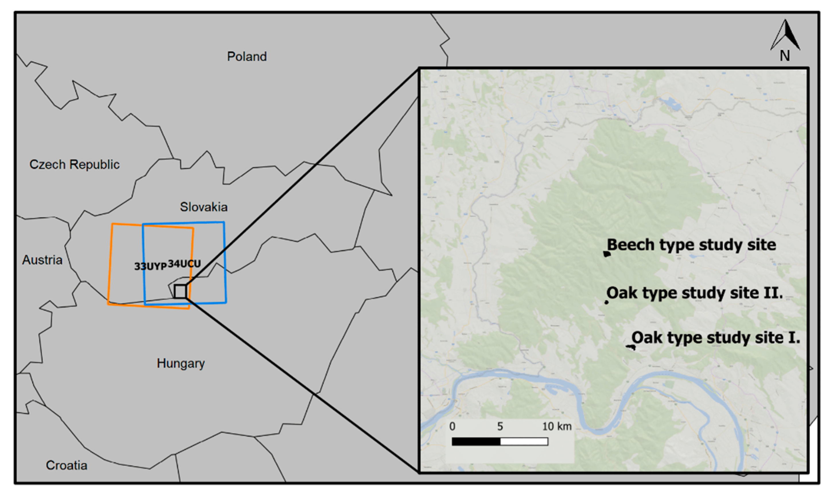
Figure 2.
OS1 with an orthophoto from 2015. The spatial resolution of the orthophoto is 0.2 m.

Figure 3.
OS2 with an orthophoto from 2015 with a spatial resolution of 0.2 m.

Figure 4.
BS with an orthophoto from 2015 with a spatial resolution of 0.2 m.
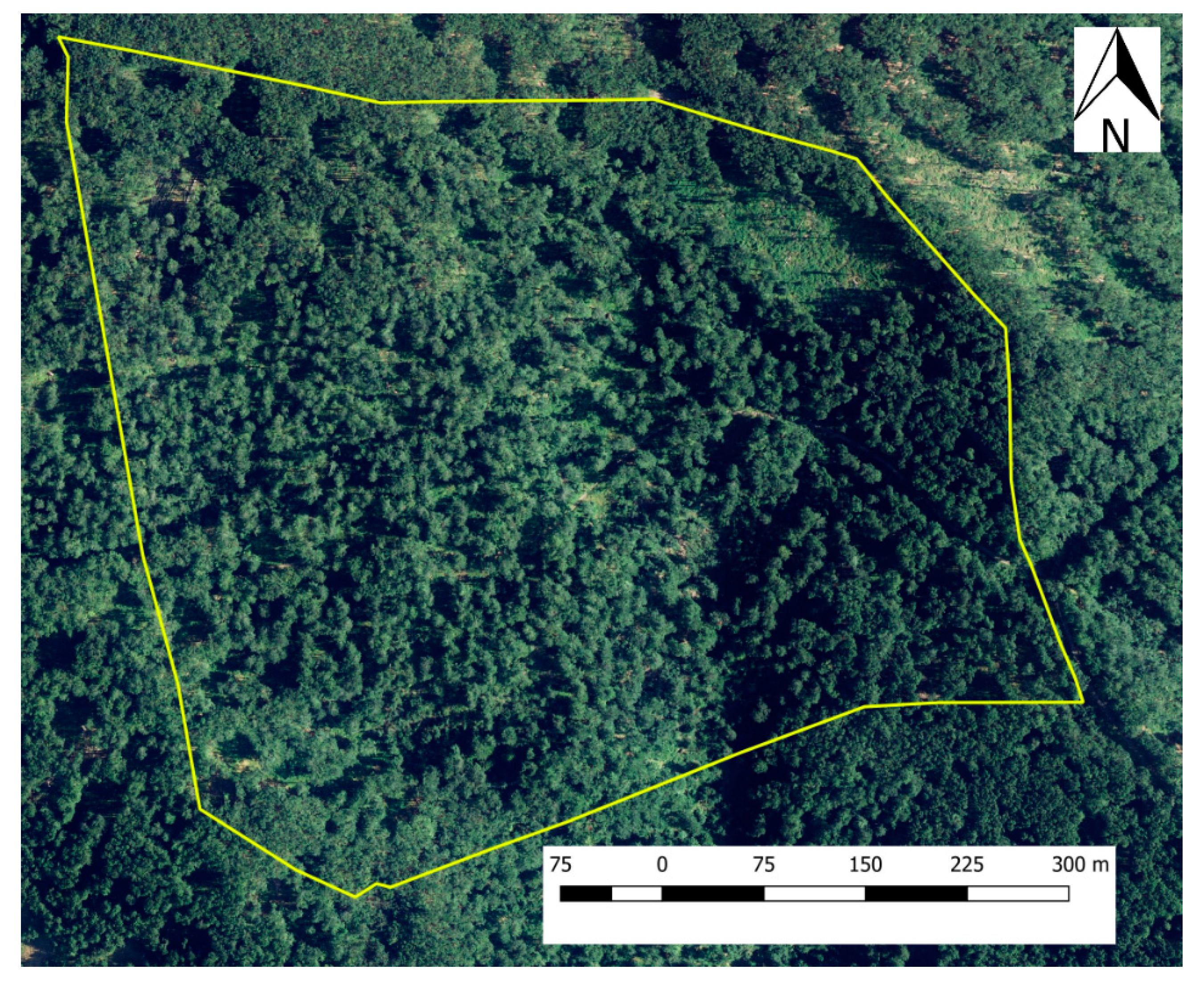
Figure 5.
The workflow chart for spectral mixture analysis.
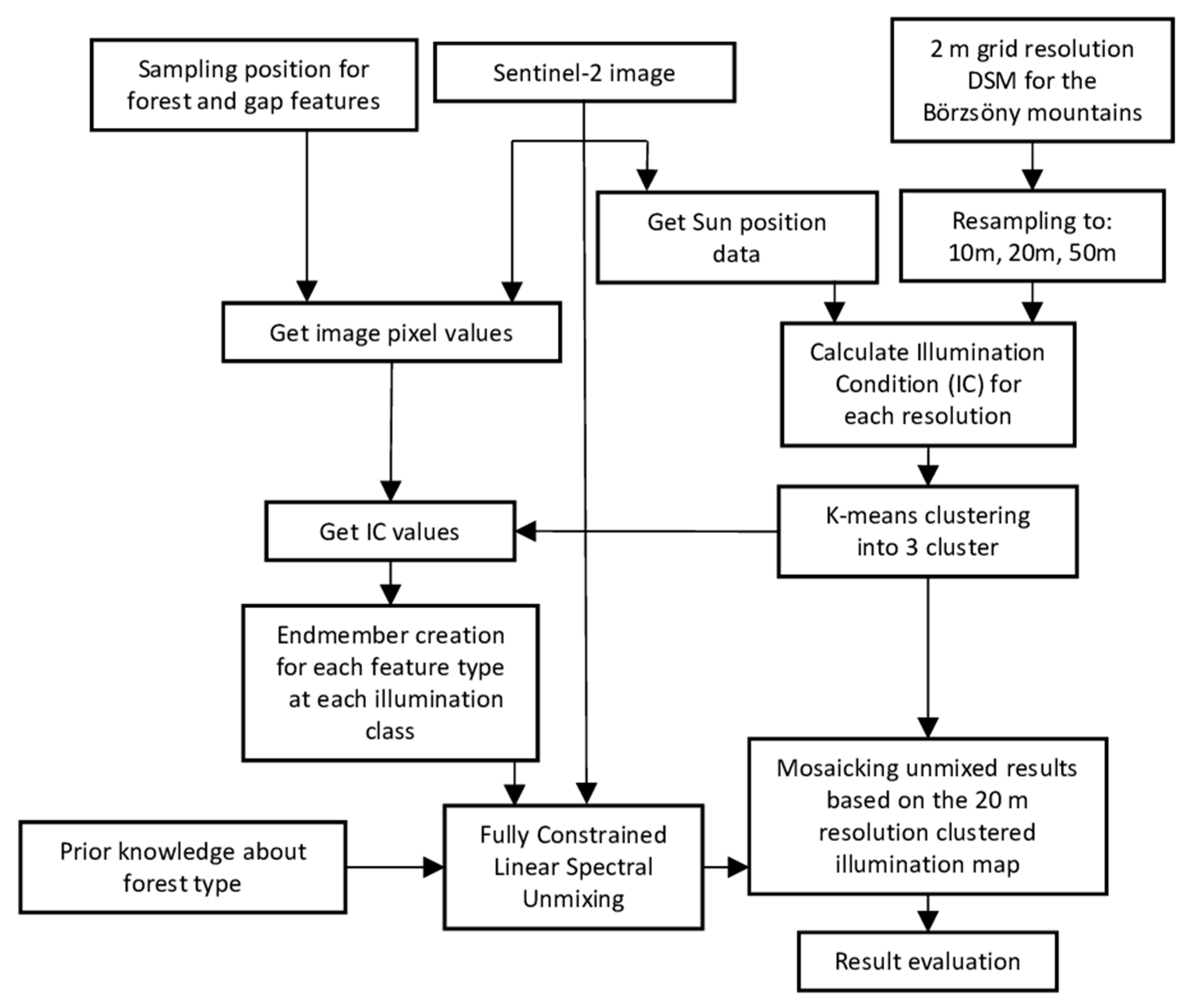
Figure 6.
The workflow chart for synthetic treefall gap modelling.
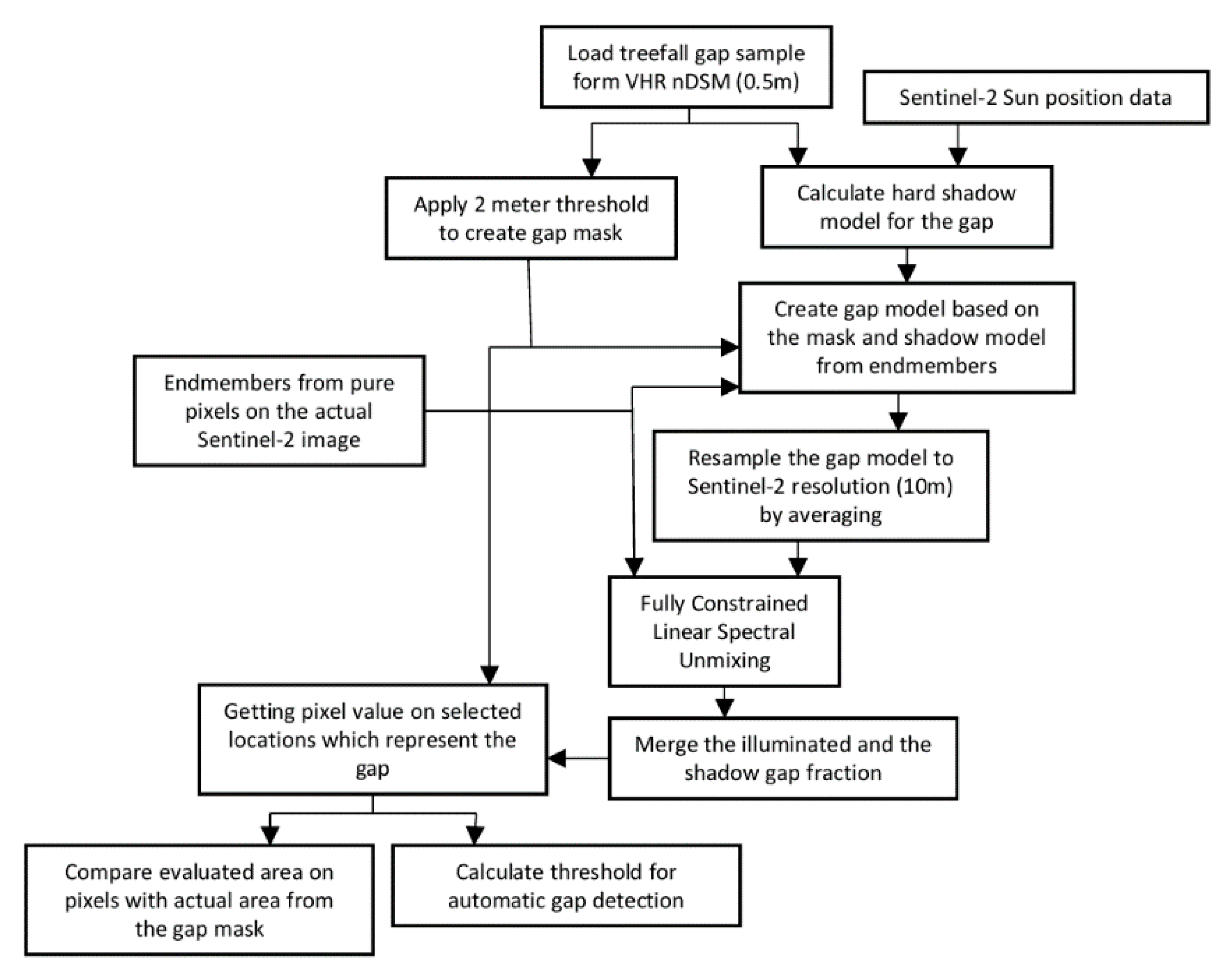
Figure 7.
Gap and Forest type endmembers from the 3 classes of illumination.

Figure 8.
Endmembers spectral profile from one illumination class.

Figure 9.
Area evaluation with randomly subsampled endmember sources on different dates.

Figure 10.
Minimum threshold value for gap fraction.

Figure 11.
Area errors on selected pixels.
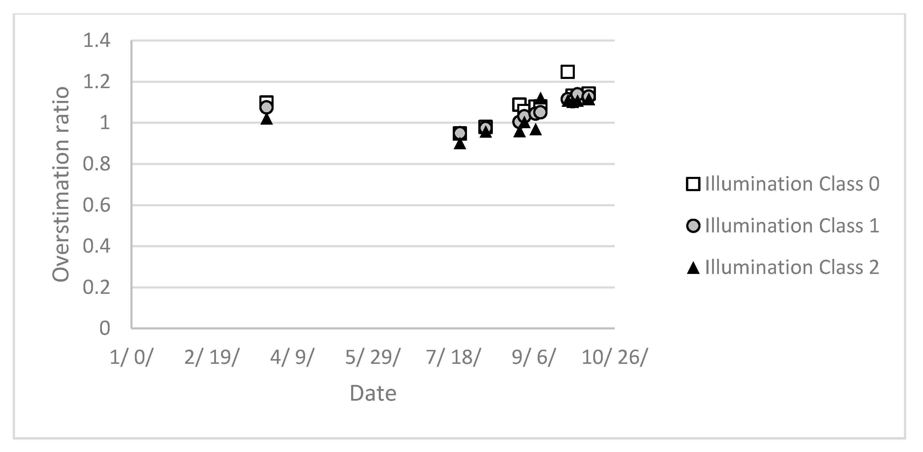
Figure 12.
Treefall gap fuzziness map evaluated from time series for 2015 (a) and 2016 (b) at the OS1 on a 10 m resolution grid. Reference treefall gap polygons shown with black outline for both years.
Figure 12.
Treefall gap fuzziness map evaluated from time series for 2015 (a) and 2016 (b) at the OS1 on a 10 m resolution grid. Reference treefall gap polygons shown with black outline for both years.
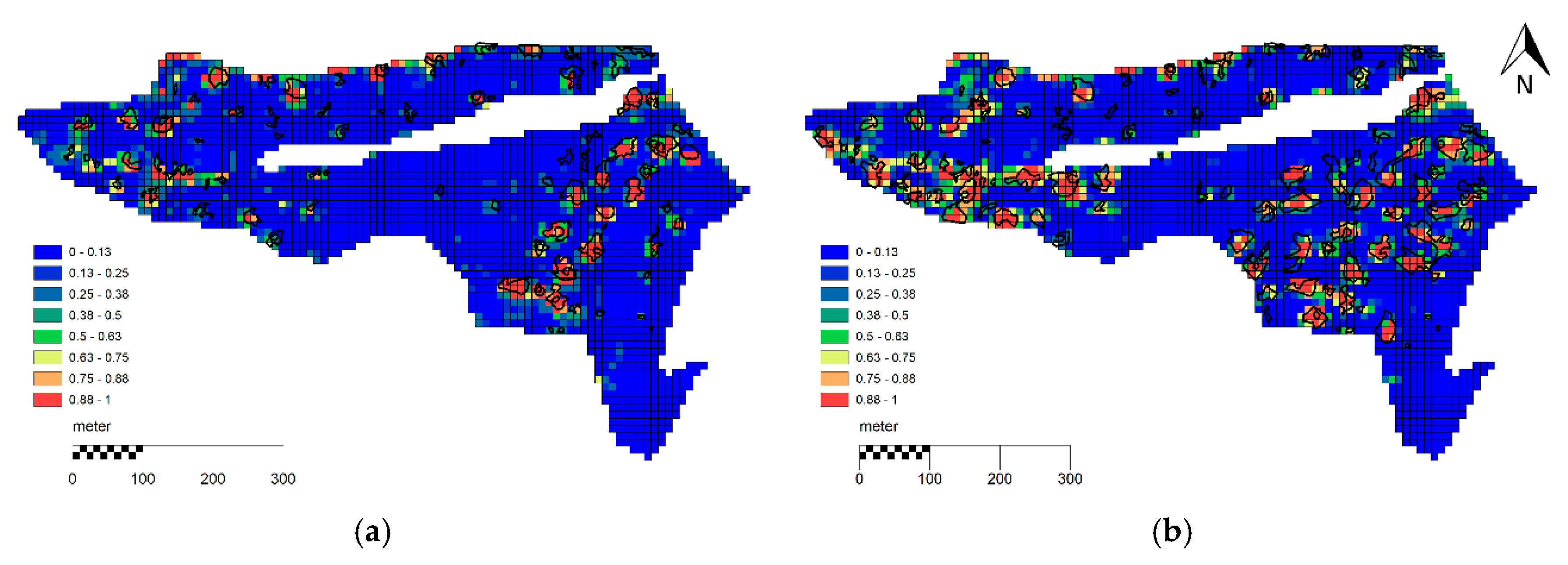
Figure 13.
Treefall gap fuzziness map evaluated from the merged time series of 2015 and 2016 at the OS2 on a 10 m resolution grid. Reference treefall gap polygons are shown with black outline.
Figure 13.
Treefall gap fuzziness map evaluated from the merged time series of 2015 and 2016 at the OS2 on a 10 m resolution grid. Reference treefall gap polygons are shown with black outline.
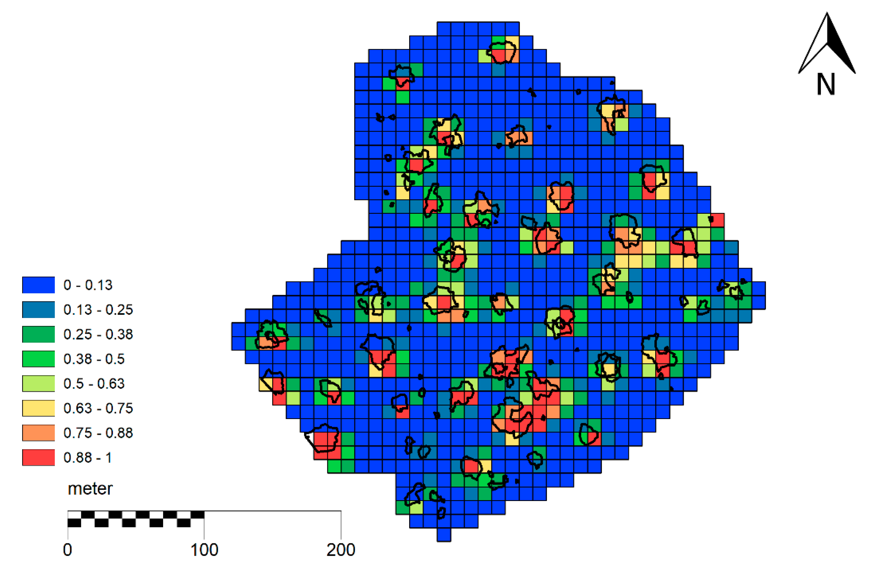
Figure 14.
Treefall gap fuzziness map evaluated from 2016 at the BS on a 10 m resolution grid (a). Regeneration strength map of partial crown damage between 2015 and 2016 on the same 10 m resolution grid (b).
Figure 14.
Treefall gap fuzziness map evaluated from 2016 at the BS on a 10 m resolution grid (a). Regeneration strength map of partial crown damage between 2015 and 2016 on the same 10 m resolution grid (b).
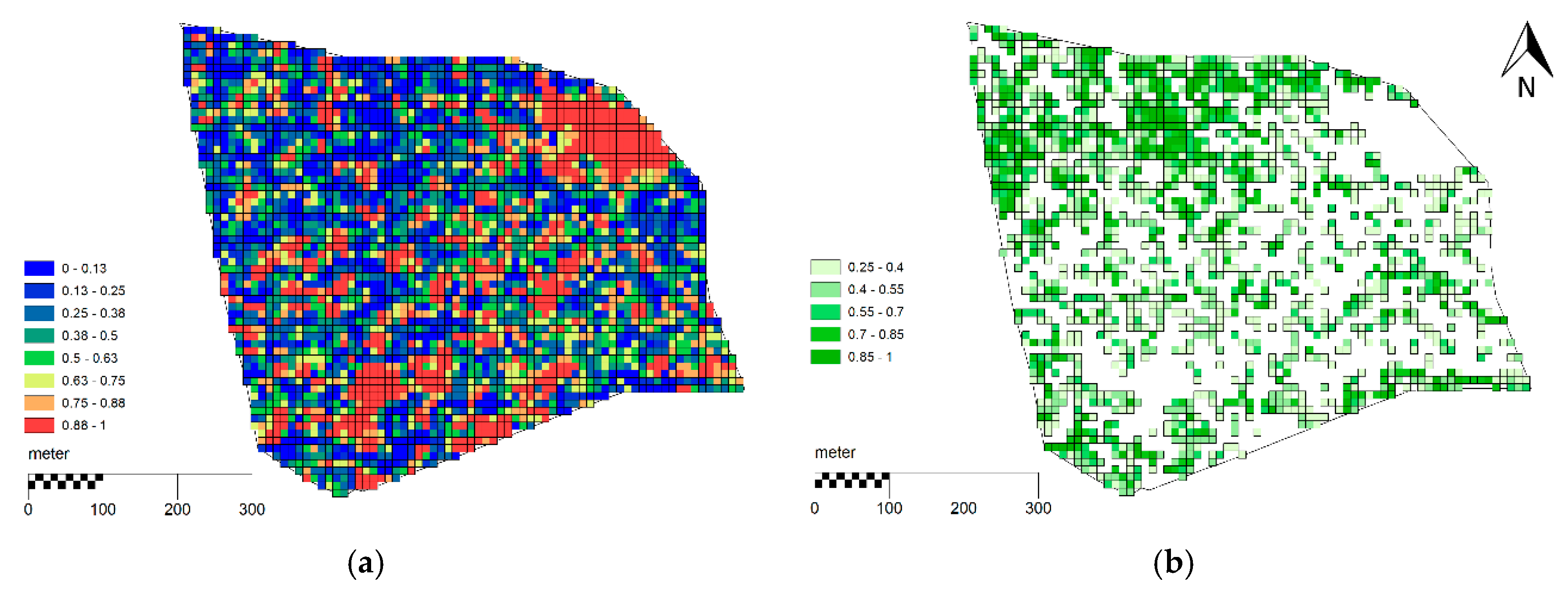
Figure 15.
Overestimation of gap size modelled on DSM (a) and the same treefall gap contour on a 0.1 m resolution color infrared orthophoto captured with lower sun elevation (b).
Figure 15.
Overestimation of gap size modelled on DSM (a) and the same treefall gap contour on a 0.1 m resolution color infrared orthophoto captured with lower sun elevation (b).

Table 1.
Details of the Sentinel-2A data.
| Satellite Path | Year | Month | Day | Sun Azimuth (°) | Sun Elevation (°) |
|---|---|---|---|---|---|
| R079 | 2015 | 08 | 07 | 156.43 | 56.68 |
| R036 | 2015 | 10 | 03 | 165.49 | 37.17 |
| R079 | 2016 | 03 | 24 | 161.83 | 42.31 |
| R079 | 2016 | 07 | 22 | 154.09 | 60.17 |
| R036 | 2016 | 08 | 28 | 157.52 | 49.64 |
| R079 | 2016 | 08 | 31 | 161.92 | 49.22 |
| R036 | 2016 | 09 | 07 | 159.99 | 46.28 |
| R079 | 2016 | 09 | 10 | 164.19 | 45.74 |
| R036 | 2016 | 09 | 27 | 164.46 | 39.09 |
| R079 | 2016 | 09 | 30 | 168.16 | 38.37 |
| R079 | 2016 | 10 | 10 | 169.69 | 34.67 |
Table 2.
Types and number of sampling positions for endmembers.
| Sample Type | Number |
|---|---|
| beech forest old | 1632 |
| beech shadowed treefall gap | 563 |
| beech forest young | 2961 |
| oak forest old | 6694 |
| oak shadowed treefall gap | 2809 |
Table 3.
Proportion of the sample positions on the images.
| Image Date | Active Sampling Positions |
|---|---|
| 7 August 2015 | 97.76% |
| 3 October 2015 | 88.34% |
| 24 March 2016 | 58.51% |
| 22 July 2016 | 62.73% |
| 28 August 2016 | 98.01% |
| 31 August 2016 | 100.00% |
| 7 September 2016 | 100.00% |
| 10 September 2016 | 100.00% |
| 27 September 2016 | 70.75% |
| 30 September 2016 | 99.99% |
| 10 October 2016 | 95.90% |
Table 4.
Correlation matrices for all endmembers from different data types.
| R | R | ||||||
| B2 | L2ADEM | L2A | L1C | B4 | L2ADEM | L2A | L1C |
| L2ADEM | 1.00 | 0.91 | 0.32 | L2ADEM | 1.00 | 0.97 | 0.78 |
| L2A | 0.91 | 1.00 | 0.31 | L2A | 0.97 | 1.00 | 0.78 |
| L1C | 0.32 | 0.31 | 1.00 | L1C | 0.78 | 0.78 | 1.00 |
| R | R | ||||||
| B3 | L2ADEM | L2A | L1C | B8 | L2ADEM | L2A | L1C |
| L2ADEM | 1.00 | 0.85 | 0.58 | L2ADEM | 1.00 | 0.88 | 0.86 |
| L2A | 0.85 | 1.00 | 0.60 | L2A | 0.88 | 1.00 | 0.95 |
| L1C | 0.58 | 0.60 | 1.00 | L1C | 0.86 | 0.95 | 1.00 |
Table 5.
Area evaluation results on OS1.
| Year | L2ADEM | L2A | L1C | Reference | |
|---|---|---|---|---|---|
| Mean (ha) | 2015 | 3.39 | 6.58 | 7.10 | 1.79 |
| 2016 | 5.04 | 8.32 | 7.85 | 3.29 | |
| SE (ha) | 2015 | 2.08 | 0.64 | 1.97 | |
| 2016 | 1.18 | 1.12 | 0.63 | ||
| Gap/Total area | 2015 | 12.92% | 25.05% | 27.03% | 6.80% |
| 2016 | 19.20% | 31.67% | 29.89% | 12.52% | |
| 2016–2015 change | ha | 1.65 | 1.74 | 0.75 | 1.50 |
| % | 6.28% | 6.62% | 2.86% | 5.71% |
Table 6.
Correlation between the treefall gap abundance rasters on different data types on different dates on OS1.
Table 6.
Correlation between the treefall gap abundance rasters on different data types on different dates on OS1.
| Date | R | ||
|---|---|---|---|
| L2ADEM-L2A | L2ADEM-L1C | L2A-L1C | |
| 7 August 2015 | 0.84 | 0.82 | 0.99 |
| 3 October 2015 | 0.58 | 0.59 | 1.00 |
| 22 July 2016 | 0.86 | 0.86 | 0.98 |
| 28 August 2016 | 0.83 | 0.82 | 1.00 |
| 31 August 2016 | 0.84 | 0.84 | 1.00 |
| 7 September 2016 | 0.81 | 0.81 | 1.00 |
| 10 September 2016 | 0.82 | 0.82 | 1.00 |
| 27 September 2016 | 0.73 | 0.78 | 0.98 |
| 30 September 2016 | 0.75 | 0.75 | 1.00 |
Table 7.
Area evaluation results on OS2.
| Year | L2ADEM | L2A | L1C | Reference | |
|---|---|---|---|---|---|
| Mean (ha) | 2015 | 1.30 | 0.76 | 1.00 | 1.24 |
| 2016 | 1.53 | 1.05 | 0.78 | 1.24 | |
| SE (ha) | 2015 | 0.21 | 0.05 | 0.10 | |
| 2016 | 0.30 | 0.28 | 0.17 | ||
| Gap/Total area | 2015 | 14.58% | 8.54% | 11.29% | 13.98% |
| 2016 | 17.23% | 11.77% | 8.83% | 13.98% | |
| 2016–2015 change | ha | 0.23 | 0.29 | −0.22 | |
| % | 2.64% | 3.24% | −2.46% |
Table 8.
Correlation between the treefall gap abundance rasters on different data types on different dates on OS2.
Table 8.
Correlation between the treefall gap abundance rasters on different data types on different dates on OS2.
| Date | R | ||
|---|---|---|---|
| L2ADEM-L2A | L2ADEM-L1C | L2A-L1C | |
| 7 August 2015 | 0.92 | 0.92 | 1.00 |
| 3 October 2015 | 0.78 | 0.77 | 1.00 |
| 22 July 2016 | 0.90 | 0.88 | 0.98 |
| 28 August 2016 | 0.87 | 0.86 | 1.00 |
| 31 August 2016 | 0.88 | 0.88 | 1.00 |
| 7 September 2016 | 0.86 | 0.86 | 1.00 |
| 10 September 2016 | 0.86 | 0.86 | 1.00 |
| 30 September 2016 | 0.82 | 0.82 | 1.00 |
| 10 October 2016 | 0.78 | 0.77 | 1.00 |
Table 9.
Area evaluation results on BS.
| Year | L2ADEM | L2A | L1C | Reference | |
|---|---|---|---|---|---|
| Mean (ha) | 2015 | 26.04 | 22.01 | 22.74 | 14.11 |
| 2016 | 21.27 | 14.69 | 14.61 | 14.11 | |
| SE (ha) | 2015 | 2.07 | 1.34 | 1.57 | |
| 2016 | 1.51 | 0.73 | 0.91 | ||
| Gap/Total area | 2015 | 79.47% | 67.18% | 69.41% | 43.06% |
| 2016 | 64.91% | 44.82% | 44.58% | 43.06% | |
| 2016–2015 change | ha | −4.77 | −7.33 | −8.14 | |
| % | −14.56% | −22.36% | −24.83% |
Table 10.
Correlation between the abundance of treefall gap rasters on different data types on different dates on BS.
Table 10.
Correlation between the abundance of treefall gap rasters on different data types on different dates on BS.
| Date | R | ||
|---|---|---|---|
| L2ADEM-L2A | L2ADEM-L1C | L2A-L1C | |
| 7 August 2015 | −0.16 | −0.11 | 0.83 |
| 3 October 2015 | 0.27 | 0.25 | 0.97 |
| 28 August 2016 | −0.17 | −0.22 | 0.96 |
| 7 September 2016 | −0.24 | −0.26 | 0.97 |
| 10 September 2016 | −0.04 | −0.26 | 0.77 |
| 30 September 2016 | −0.27 | −0.38 | 0.88 |
Table 11.
Evaluated area from time series on OS1.
| L2ADEM | Reference | Reference + 2.0 m Buffer | |
|---|---|---|---|
| Area 2015 (ha) | 3.33 | 1.76 | 3.18 |
| Area 2016 (ha) | 5.19 | 3.26 | 5.32 |
| Area 2015 + 2016 (ha) | 5.39 | 3.26 | 5.32 |
Table 12.
Evaluated area from time series on OS2.
| L2ADEM | Reference | Reference + 2.0 m Buffer | |
|---|---|---|---|
| Area 2015 (ha) | 1.43 | 1.24 | 1.67 |
| Area 2016 (ha) | 1.81 | 1.24 | 1.67 |
| Area 2015 + 2016 (ha) | 1.72 | 1.24 | 1.67 |
Table 13.
Evaluated area from time series on BS.
| L2ADEM | Reference | |
|---|---|---|
| Area 2015 (ha) | 23.03 | 14.11 |
| Area 2016 (ha) | 15.49 | 14.11 |
| Area 2015–2016 (ha) | 7.54 |
© 2017 by the authors. Licensee MDPI, Basel, Switzerland. This article is an open access article distributed under the terms and conditions of the Creative Commons Attribution (CC BY) license (http://creativecommons.org/licenses/by/4.0/).
Share and Cite
MDPI and ACS Style
Barton, I.; Király, G.; Czimber, K.; Hollaus, M.; Pfeifer, N. Treefall Gap Mapping Using Sentinel-2 Images. Forests 2017, 8, 426. https://doi.org/10.3390/f8110426
AMA Style
Barton I, Király G, Czimber K, Hollaus M, Pfeifer N. Treefall Gap Mapping Using Sentinel-2 Images. Forests. 2017; 8(11):426. https://doi.org/10.3390/f8110426
Chicago/Turabian StyleBarton, Iván, Géza Király, Kornél Czimber, Markus Hollaus, and Norbert Pfeifer. 2017. "Treefall Gap Mapping Using Sentinel-2 Images" Forests 8, no. 11: 426. https://doi.org/10.3390/f8110426
Note that from the first issue of 2016, this journal uses article numbers instead of page numbers. See further details here.