An Examination of Diameter Density Prediction with k-NN and Airborne Lidar
by
Jacob L. Strunk
1,*, 
Peter J. Gould
2,
Petteri Packalen
3,
Krishna P. Poudel
4,
Hans-Erik Andersen
1 and
Hailemariam Temesgen
4 1
USDA Forest Service Pacific Northwest Research Station, University of Washington, P.O. Box 352100, Seattle, WA 98195-2100, USA
2
Washington State Department of Natural Resources, P.O. Box 47000, 1111 Washington Street SE, Olympia, WA 98504-7000, USA
3
Faculty of Science and Forestry, University of Eastern Finland, P.O. Box 111, 80101 Joensuu, Finland
4
Department of Forest Engineering, Resources and Management, Oregon State University, Corvallis, Peavy 204, OR 97331-5706, USA
*
Author to whom correspondence should be addressed.
Forests 2017, 8(11), 444; https://doi.org/10.3390/f8110444
Submission received: 29 September 2017
/
Revised: 30 October 2017
/
Accepted: 10 November 2017
/
Published: 16 November 2017
(This article belongs to the Section Forest Inventory, Modeling and Remote Sensing)
Abstract
:While lidar-based forest inventory methods have been widely demonstrated, performances of methods to predict tree diameters with airborne lidar (lidar) are not well understood. One cause for this is that the performance metrics typically used in studies for prediction of diameters can be difficult to interpret, and may not support comparative inferences between sampling designs and study areas. To help with this problem we propose two indices and use them to evaluate a variety of lidar and k nearest neighbor (k-NN) strategies for prediction of tree diameter distributions. The indices are based on the coefficient of determination (R2), and root mean square deviation (RMSD). Both of the indices are highly interpretable, and the RMSD-based index facilitates comparisons with alternative (non-lidar) inventory strategies, and with projects in other regions. K-NN diameter distribution prediction strategies were examined using auxiliary lidar for 190 training plots distribute across the 800 km2 Savannah River Site in South Carolina, USA. We evaluate the performance of k-NN with respect to distance metrics, number of neighbors, predictor sets, and response sets. K-NN and lidar explained 80% of variability in diameters, and Mahalanobis distance with k = 3 neighbors performed best according to a number of criteria.
1. Introduction
Airborne scanning lidar technology (henceforth referred to as simply lidar) provides vegetation measurements which are highly related to forest attributes needed for forest inventory and monitoring. Some examples of forest attributes which are highly related to lidar measurements include stem volume, basal area, quadratic mean diameter, and above-ground biomass [1,2,3]. The lidar vegetation measurements can be obtained with high precision over large areas enabling wall-to-wall measurements and predictions of vegetation attributes, as well as precise estimates of population parameters. Despite demonstrated advantages to using lidar for inventory and monitoring, there are also omissions from most analyses which inhibit common usage. One of the limitations of typical lidar research studies, is that they do not directly evaluate prediction of tree diameter distributions.
The distribution of diameters at breast height (dbh) is an important component of most forest inventory, management, and monitoring strategies. Dbhs are needed to describe stand properties because variables such as growth, volume, market value, conversion-cost, product specifications, and future forest prescriptions are dependent on trees’ dbhs. The use of single-tree level growth and yield models almost always requires dbh distributions. Dbhs are also used to assess forest sustainability based on whether the quantity and sizes of growing stock are suited to replace the current population of harvestable trees [4]. Information about dbhs also informs the type and timing of management strategies and economic value of the stand [5]. Ecological analyses also use dbh density information including, for example, assessments of vegetative diversity [6], insect disturbance mechanics [7], habitat suitability [8], and suitability and distribution of parent stock for coarse woody debris [9].
Dbh distributions are often simplified using a mathematical function with parameters that can be estimated or recovered using lidar measurements or other ancillary data. Dbh distribution functions can be predicted with both parametric and non-parametric strategies. Parametric strategies are based on the assumption that the dbh density can be characterized by a theoretical probability density function. A variety of theoretical functions have been tested including the beta [10], Weibull [11,12] and Johnson’s SB [13,14]. Two methods have been used to predict parameters of theoretical functions, the parameter prediction method and the parameter recovery method [15]. As the name indicates, in the parameter prediction method stand attributes (or remote sensing data) are used to predict parameters of the probability density function. In the parameter recovery method moments or percentiles of dbh distribution are predicted or measured using stand variables. The parameters of a theoretical distribution are then recovered by leveraging the known relationships between the predicted attributes and the distributional parameters.
Non-parametric strategies attempt to predict percentiles of empirical distributions [16,17] or directly predict dbh bins or classes. While parametric strategies are advantageous in being able to represent a complete distribution with a few parameters when the empirical distribution is unimodal, they may have limited ability to represent complex and mixed species stands that may not have unimodal densities [18]. Empirical strategies which retain the original data or relative densities by dbh bins provide more flexibility to accommodate many types of stand tables [17], however, some prediction strategies for multiple dbh percentiles can result in illogical behavior, benefitting from the introduction of constraints [19].
Various strategies for predicting dbh distributions with lidar have been evaluated. Gobakken and Næsset [20] compared parameter prediction and parameter recovery methods in the prediction of stem number and basal area distributions. The underlying probability theoretical distribution was a two-parameter Weibull distribution. The precision was slightly better for the parameter recovery method than for the parameter prediction method. Mehtatalo et al. [21] also used the parameter recovery approach, however, they proposed a method where the parameters of the assumed dbh distribution and height-dbh curve are determined in such a manner that they are compatible with the predictions of stand attributes. Maltamo et al. [22] proposed another approach to obtain a compatible stand description. First the parameters of a Weibull distribution and stand volume are predicted with lidar. Then, the estimated stem number distribution is modified to correspond to the volume obtained in the previous step by using the calibration estimation approach proposed by Deville and Sarndal [23].
Percentiles of dbh distributions have also been predicted with lidar. Maltamo et al. [24] predicted 12 percentile points in semi-natural forests in Finland. Bollandsås and Naesset [25] predicted 10 percentiles in uneven-sized Norway spruce stands. Breidenbach et al. [26] used a generalized linear model (GLM) to estimate parameters of theoretical distributions with lidar. A benefit of GLM is that they can be a one-step procedure, without the need to first fit a distribution and then predict its parameters. Thomas et al. [27] studied the prediction of both unimodal and bimodal dbh distributions using a finite mixture model approach. They successfully predicted the parameters of separate Weibull functions, but because there was no lidar-based method for separation of distribution type (unimodal or bimodal), the applicability of the method is somewhat limited for lidar inventory.
An alternative strategy to predict dbh distribution with lidar is using k-nearest-neighbor (k-NN) imputation. An advantage of k-NN is that the k-NN model can be used to simultaneously predict a suite of response variables, including a list of individual trees records (tree-list). k-NN also provides compatible stand if stand attributes are predicted simultaneously with tree-lists. This was the motivation for the work by Packalén and Maltamo [28]. They predicted stand attributes and tree-lists simultaneously for Scots pine, Norway spruce, and deciduous trees and compared the performance of a tree-list approach to the use of a Weibull distribution approach. The k-NN tree-list strategy was able to mimic bimodal dbh distributions of Norway Spruce (the only shade tolerant tree species in the study area) and in general provided clearly lower error index values. Maltamo et al. [29] examined the performance of a k-NN tree-list approach without considering tree species. Their objectives were to investigate the effect of different predictor and response variables and to examine the influence of reduced numbers of training plots. The results indicated that response variables must be selected very carefully in order to obtain accurate predictions of dbh distributions and stand attributes. They also reported that with a low number of training plots (approx. 100) precise predictions of dbh distributions could be produced in their study area.
When a diameter prediction strategy is evaluated, inference is typically made on differences between the observed and predicted distribution using hypothesis or goodness of fit tests, such as the Kolmogorov-Smirnov test. However, for reasons described extensively in Reynolds et al. [30] including that the p-values can be wildly inaccurate (for fewer than 40 trees per plot), these types of tests are problematic for many of the same reasons that the statistical community discourages p-value based inference in hypothesis testing (e.g., Halsey et al. [31]). Reynolds et al. [30] instead proposed an index based upon absolute deviations in the units of the response. This index is often referred to as the “Reynolds error index” in the literature. Reynolds et al. [30] also described methodologies for formal statistical inference using their error index.
In this study we wished to understand tradeoffs between various lidar and k-NN based dbh prediction strategies (e.g., numbers of neighbors, distance metrics, and others). While studies have examined dbh predictions with lidar, only a subset of prediction strategies were examined, and the indices used by studies are difficult to generalize to other designs and areas. To overcome these limitations, we propose two indices and use them to examine a variety of dbh predictions strategies. The proposed indices are based on the well-known coefficient of determination (R2), and root mean squared deviation (RMSD) which simplifies their interpretation by users and readers.
Initially, we graphically demonstrate the behavior of the two proposed indices using simulations. We then use the indices to describe the relative performances of a variety of lidar and k-NN diameter distribution prediction strategies. Given the large number of components of a k-NN and lidar prediction strategy, clarity is needed on which k-NN configurations work best with lidar for dbh distribution predictions. Components that we examine include distance metrics (e.g., Euclidean vs. Mahalanobis), numbers of neighbors (the k in k-NN), presence or absence of stratification, and sensitivity of predictions to the choice of response and predictor variables. Based on our findings using the proposed indices, we conclude with recommendations on effective diameter distribution predictions strategies with lidar and k-NN.
2. Materials and Methods
2.1. Study Site
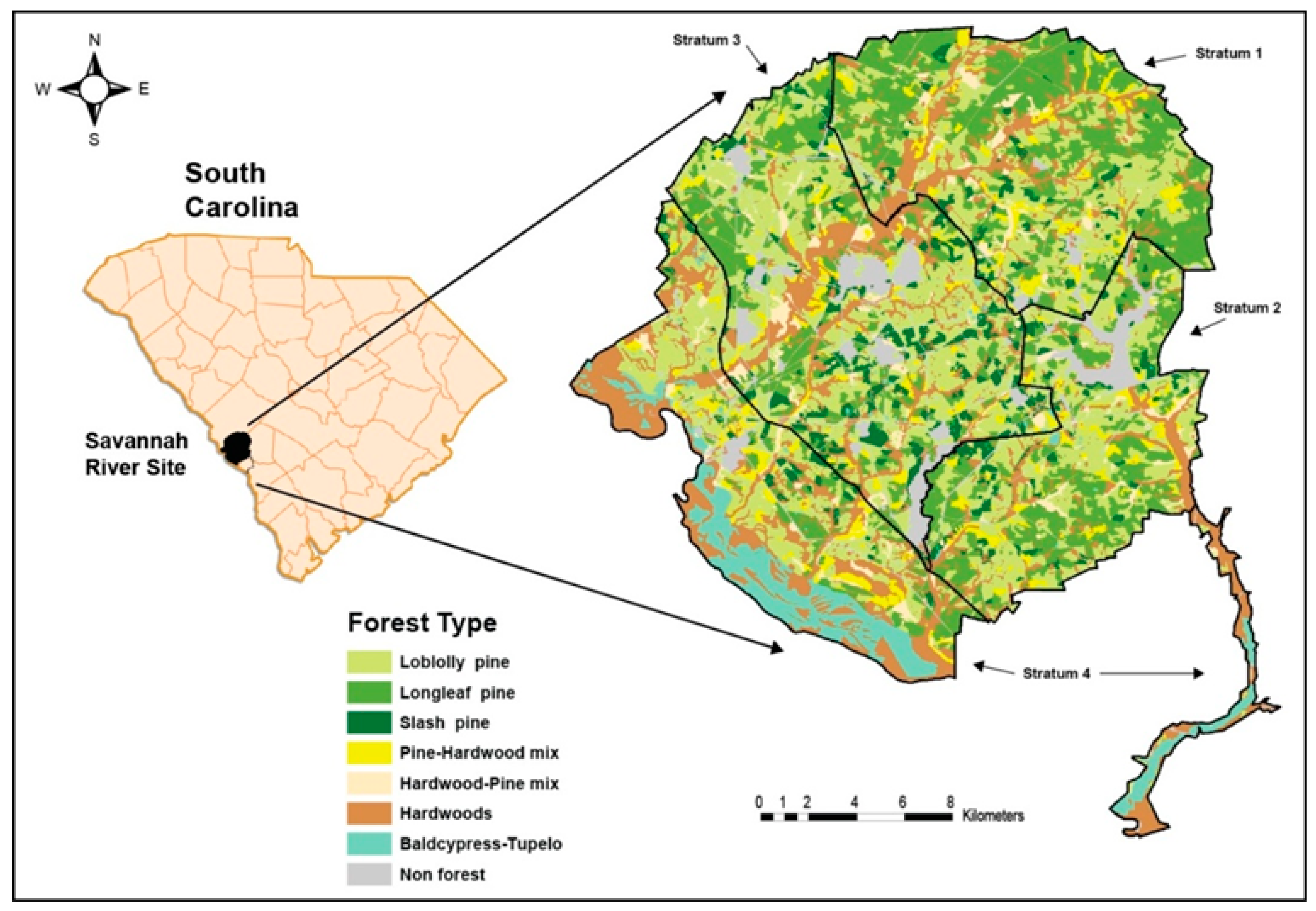
The study was conducted at the U. S. Department of Energy’s Savannah River Site, an 80,267 ha National Environmental Research Park in Aiken and Barnwell counties, South Carolina USA (Figure 1). The Savannah River Site is characterized by sandy soils and gently sloping hills dominated by pines, with hardwoods occurring in riparian areas. Prior to acquisition by the Department of Energy in 1951, the majority of Savannah River Site uplands were agricultural fields or had recently been harvested for timber. The U.S. Department of Agriculture Forest Service has managed the natural resources of the Savannah River Site since 1952 and reforested the majority of the uplands with loblolly (P. taeda), longleaf (P. palustris), and slash (P. elliottii) pines. These pine stands are actively managed for timber and wildlife habitat.
2.2. Ground Data Collection
Plot measurements were performed on a grid of fixed radius circular plots designed for modeling forest attributes with auxiliary lidar data. The plot design consisted of two concentric nested fixed area circular measurement plots. The innermost 0.004 ha plot was used to measure trees between 2.5 and 7.4 cm in dbh. Larger trees were measured on a 0.04 ha plot if there were at least 8 dominant or co-dominant trees, otherwise trees larger than 7.4 cm dbh were measured on a 0.081 ha plot. The heights, dbhs, heights to crown base, and species were recorded for trees on the two concentric plots, and additionally trees between 2.5 and 7.4 cm were tallied on a 0.04 ha plot.
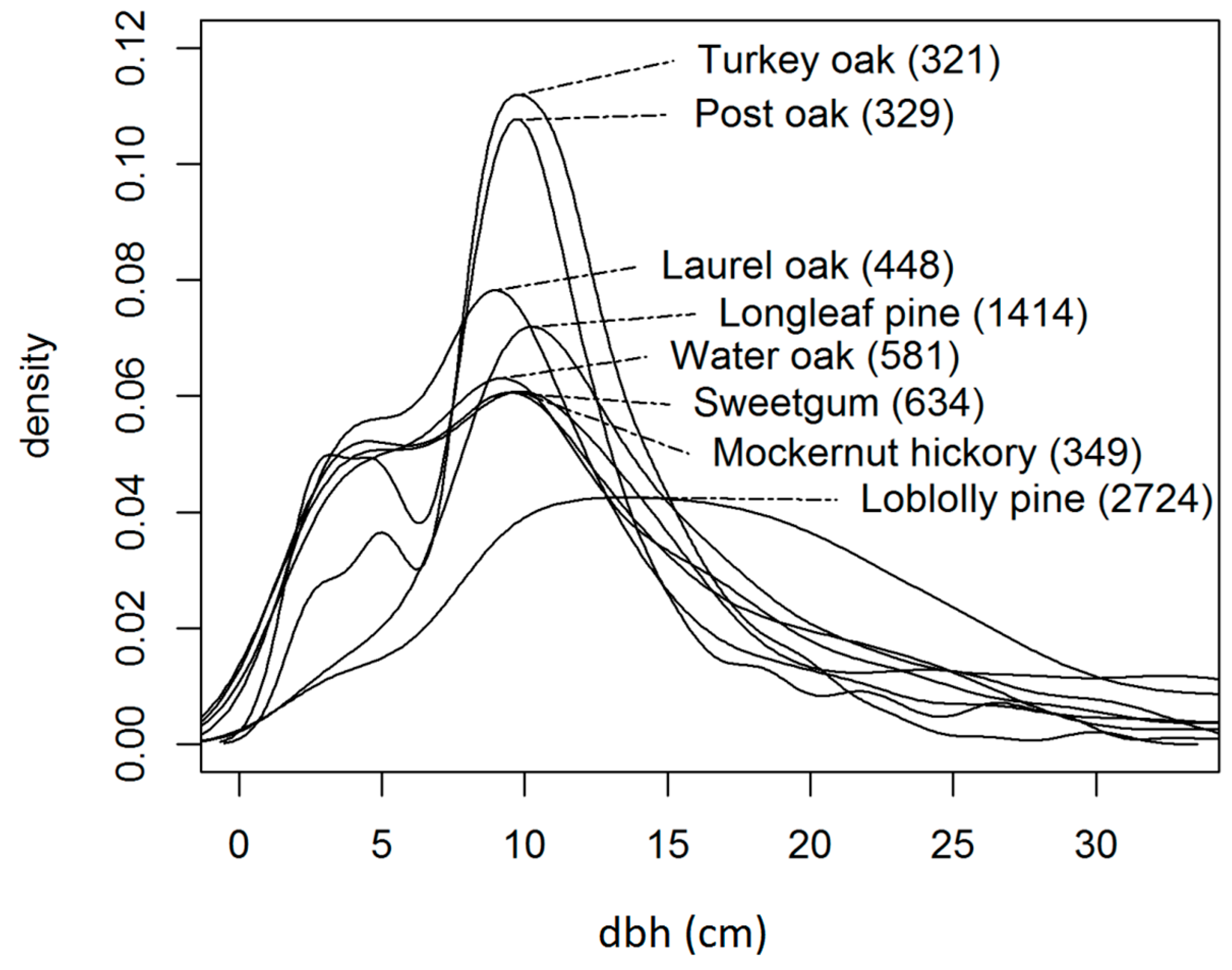
Plot locations were selected purposively to cover the range of tree sizes and stand compositions that occur on the Savannah River Site. Field measurements were taken on 194 field plot locations selected purposively to sample across multiple vegetation classes and sizes. Of the 194 plots, 4 were dropped because it was determined that they were measured in locations outside of our target population. A summary of the tree and plot variables used for this study is provided in Table 1. Additionally, a visual representation of the empirical dbh density functions for the 8 most common species occurring on plots is shown in Figure 2. Additional forest attributes (besides dbh) used in our analyses included trees per hectare (TPH), basal area per hectare (m2/ha, BA), Lorey’s height (m, Lor.), and total cubic stem volume (m3/ha, Vol.).
Plot locations were surveyed using L1/L2 GLONASS enabled survey-grade GPS receivers. The receiver was placed at each plot’s center on a 3 m pole and a minimum of 600 1-second-epoch satellite fixes were collected and differentially corrected. We expect the horizontal RMSE for surveyed plot center positions to be less than 1 m in the pine forest types at the Savannah River Site, based upon our previous experience with positional accuracy using these receivers in a variety of forest types (e.g., Andersen et al. [32]).
Plots were assigned to post-strata using the dominant species group for the stand in which the plot was measured (the most common dominant types include: Hardwood—29 plots; Loblolly P.—76 plots; Longleaf P.—54 plots). All of the hardwood species were combined into a single stratum. Forestry staff for the site developed a tract-wide map of species groups by visually classifying stands in the field. Plots were assigned to strata by intersecting plot locations with the strata map.
2.3. Lidar Data
Lidar data were collected from 21 February to 2 March 2009 with two Leica ALS50-II lidar sensors in leaf-off conditions. Table 2 provides acquisition parameters.
Point cloud data were processed to create predictor variables for this study using the cloudmetrics executable included with FUSION software [33]. This executable computes a large number of statistics from lidar including, but not limited to, height percentiles (e.g., 90th, 50th, and 30th percentile heights in Table 3) and lidar cover (the percent of returns above a threshold, in our case 1.50 m). We also examined fraction without foliage (fwof), a modeled variable which used normalized intensity to suggest the proportion of the leaf-off lidar which did not intersect live foliage.
2.4. k-NN Tree-List Imputation
In k-NN imputation, response variables from measured sites are shared or imputed with sites without measurements based on the degree of similarity in their auxiliary variables. The “similarity” in auxiliary variables is evaluated using a distance metric, e.g., Euclidean distance, where a large number of distance metrics have been demonstrated in the k-NN literature. The distance metrics are functions which determine how one or more auxiliary variables should be weighted and combined. The coefficients of the weight function can also depend on the observed association between response and predictor variables, theoretically weighting predictors which can better predict the response variable(s). If more than one nearest neighbor (k greater than one) is used, then a rule must be formulated to average (continuous) and select (categorical) donor response values. This procedure can be used to simultaneously impute a large number of response variables in a single step.
Procedurally, the process is as follows: (1) a distance metrics is computed between measured and unmeasured (response) observations, then (2) the k observations with the smallest distances (donors) are transferred (imputed) to the observation without a measured response (target).
For this study we relied upon the yaImpute package [34] implemented in R [35] for k-NN imputation. The identities of the donor plots (nearest neighbors) were used to impute tree-lists, as yaImpute is not currently set up to directly impute tree-lists. Based on the donors’ identities, all of the tree records from the imputed donor plots were copied to the target observation. Each copied tree was then distance weighted to generate a tree-list for the target observation. The distance weighted tree-lists from the k neighbors then became the basis for prediction of the empirical dbh density for the target observation. The choice of a weighting function for the K imputed neighbors has been shown to have limited effect on performance [28].
2.5. k-NN Imputation Strategy Components
We examined the effects of 4 components of a k-NN tree-list imputation strategy including (1) the choice of distance metric, (2) the selected predictors, (3) the set of response variables, and (4) the effect of post-stratification. The distance metrics evaluated include Euclidean distance (EUC.), Mahalanobis distance (MAH), most similar neighbors (MSN), and random forest (RF). MSN and RF distances both use response variables for measured observations in computing distances. Additional details for how these distances are defined can be found in the yaImpute package documentation [34]. The effect of post-stratification on k-NN performance was evaluated by stratifying the data, and predicting separately within strata. Strata with fewer than 10 response measurements were imputed from the pool of all observation.
2.6. Dbh Densities
The proportions of trees falling in diameter bins (the empirical dbh density, or just “dbh density”) were computed by first binning lists of trees into 2.54 cm (1 inch) dbh bins and computing the proportions of all trees in the dbh classes. In the case of imputed tree-lists, weighted dbh densities were computed using the distance weights from the imputed plots. The bin proportions were then smoothed with a 3-bin moving average centered on the target bins. The smoothing function was applied to emphasize major trends, and de-emphasize fine-scale fluctuations. Individual plot densities can have spikes, pits, and other characteristics that we did not wish to examine.
2.7. Measures of Performance
Evaluation of k-NN predictions strategies were performed using Leave One Out (LOO) validation in combination with indices. In LOO, models are iteratively fit to the data while omitting one plot at a time. After fitting a given model, the data are then tested against the omitted plot. The errors in prediction for the omitted plots then serve as the basis for indices of performance. Our first suggested measure of performance is index H.
Index H is equivalent to the coefficient of determination (or, commonly, R2) which has a straight-forward interpretation—the proportion of variability explained. The index has an advantage over alternative measures of performance that we examined in that it provides a relative measure of performance. The baseline level of variability comes from plot variation in dbh densities around the mean dbh density within a dbh class for all of the plots. As with R2, smaller prediction error relative to baseline variability will yield index H values closer to one. Larger prediction residuals will in general cause index H to approach zero, and negative values of H are possible if the prediction strategy is inferior to prediction with the means model. Our inferences for this index are similar to those that would be made from R2. We rely heavily on index H for inferences about different k-NN dbh prediction strategies. While the H values are suggestive of general trends in performance, the index is not suited for identifying a single best prediction strategy.
A limitation of index H is that it is only meaningful in comparisons if the baseline variability is similar between compared strategies. In many cases this property will not hold. We expect, for example, to have greater variability amongst variable radius plots than amongst fixed radius plots for the same area; comparing their index H values then would be meaningless. To compare prediction strategies from two different inventory designs or two study areas with different levels of baseline variability, it is important to have an absolute measure of performance. A second limitation to index H is that the index is unitless, and it is often desirable to have an index in the same units as the attribute of interest. To support inferences from multiple designs in the units of the response, we propose a second index, I, which is an absolute measure of performance:
Index I is equivalent to the Root Mean Squared Deviation (RMSD) by plot (rather than by bin). The units for this index are the same as for the attribute of interest. As with RMSD, a smaller value of index I indicates better prediction performance. Index I can be used to compare performance across sites, designs, and project areas.
While we do not use p-values in this analysis, we recognize that some users will wish to use p-values. p-value can be fairly easily generated for the suggest indices with simulations. One simulation-based approach to obtain p-value is to randomly assign tree-lists to plots several thousand times, and compute index values for each randomization. This will yield a distribution of index values for the null model where lidar and k-NN provide no explanatory power. The distribution can then be compared to the observed index value for a particular lidar and k-NN configuration. The proportion of values which are as extreme as the observed index value will serve as the simulation-based p-value.
2.8. Index Demonstration
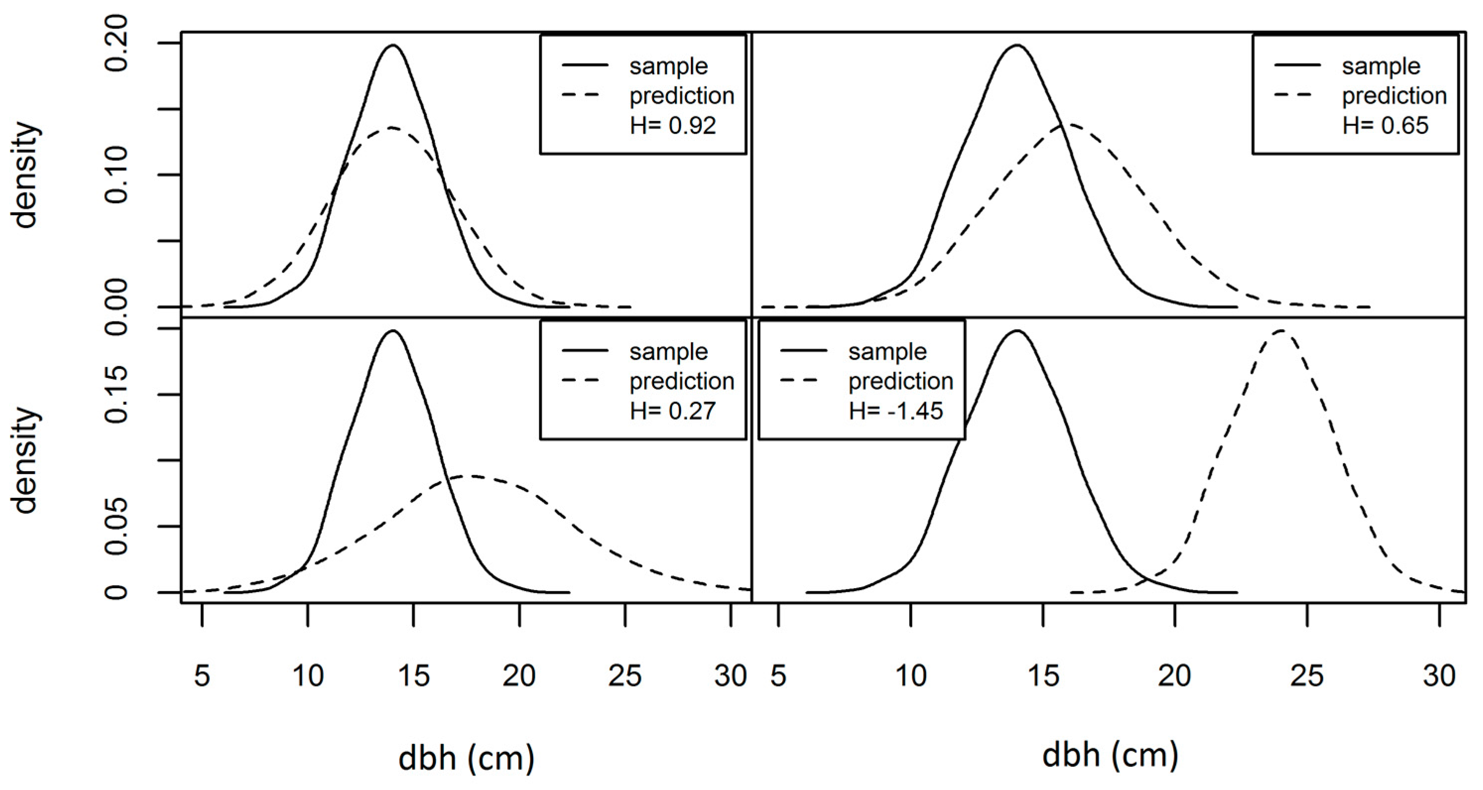
To provide a sense of the behavior of our indices as a function of prediction performance, we provide a visual calibration image which shows H values for various levels of departure from agreement between a sample and a prediction (Figure 3). Our quantitative examination of the properties of H relative to prediction properties used simulated dbhs. Our simulated population is a mixture distribution composed of two normal distributions (the solid line in Figure 4). For our examination, we took 100 clustered sample plots of 50 trees from the simulated population, and compared these with “predictions” for the samples. In Figure 4 we can see all three cases: (1) the underlying population, (2) the distribution observed on a plot, and (3) the prediction for the plot. For the purposes of demonstration, predictions were obtained by taking the original sample data and introducing Gaussian noise with parameters (). In our simulations, we look at various dbh bin widths and four types of errors in our predictions, where the four types of prediction errors are represented as four separate lines and labeled with the parameters of their error distributions. Larger values of index H suggest better prediction performance, where H is bounded by one on its upper end. A value less than zero indicates that the mean by bins (as obtained from all sample plots) is a better predictor of the sample distribution than the prediction strategy under examination.
3. Results
Results are divided into two sections. In the first section—Index properties—we demonstrate the behavior of H under a variety of prediction scenarios. Our demonstration of index H gives a sense of the behavior of H under various conditions, and the degree of sensitivity of the index to disagreement between predicted and observed dbhs. Simulation results are shown only for index H (not I) for the sake of brevity, since the behavior of the two indices is nearly identical (inversely), although the interpretations are quite different: index H provides a measure of relative improvement over the mean model (higher is better), and index I provides a measure of absolute error in the units of the response that is portable between designs and studies (lower is better).
In the second section—K-NN strategies—we use index H to suggest superior dbh prediction strategies, then conclude with a table of H and I values for the best prediction strategies. We investigate number k of nearest neighbors, which distance metric is used, which sets of predictors and response variables are used for k-NN imputation, and how are predictions for individual species. As with R2, higher index H values suggest better prediction performance, but are not necessarily suited for model selection. Instead, they are meant to help interpret general trends in performance for different prediction configurations.
3.1. Index Behavior
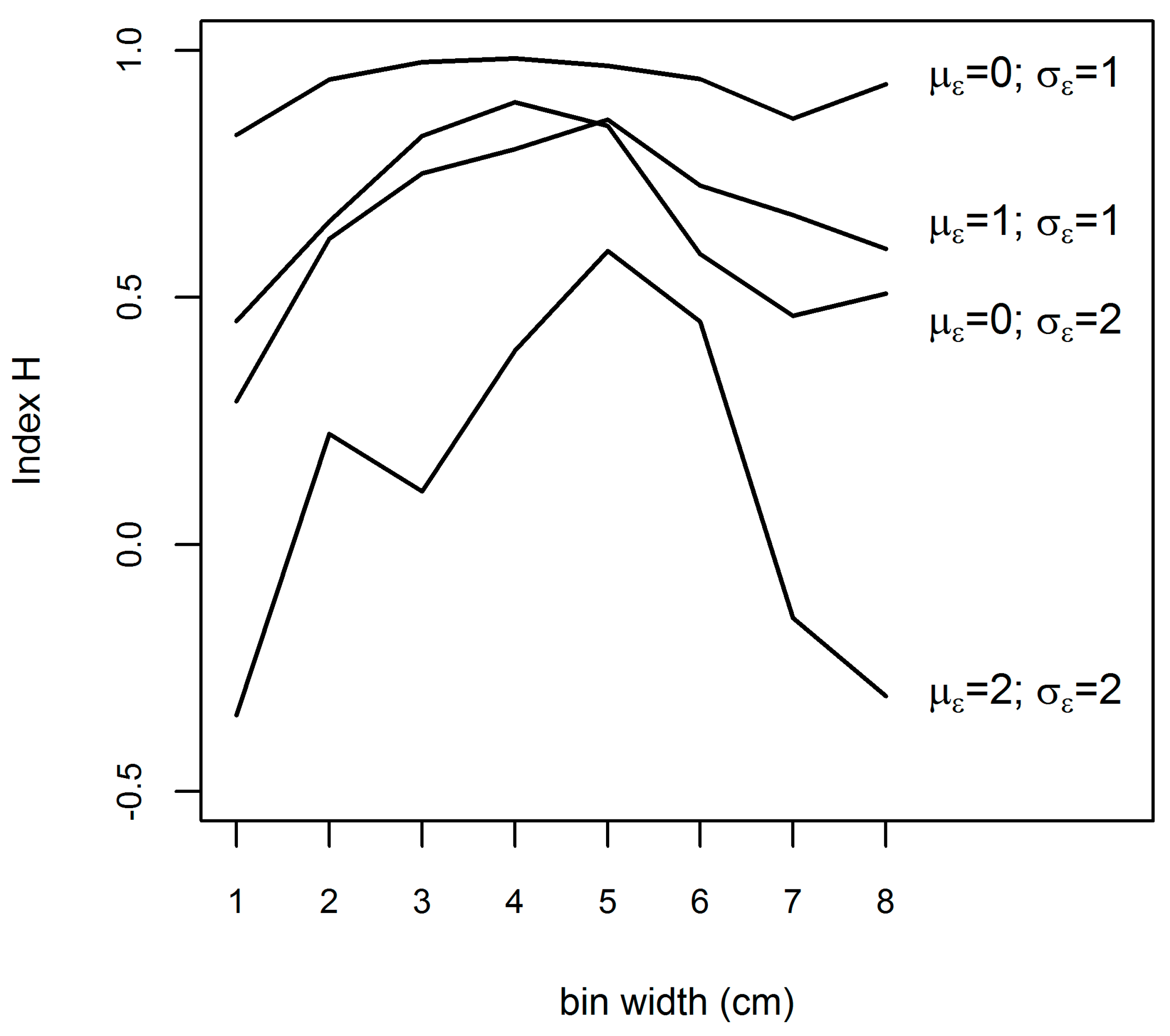
In Figure 5 we can see that the effect of bin width on H was observed similarly for each type of prediction error. In each instance both small and large dbh bin widths have reduced values of H, with the highest (best) values of H typically occurring around 4 to 5 cm for our simulations. We can expect lower values of H for small bins because there are few observations in narrow bins, resulting in higher sampling variability in both the plot sample and the plot predictions for each bin. We can also expect lower values of H for larger dbh bins because the shape of the dbh distribution approaches the average density for the plot. In this case (large dbh bins), plot mean densities have greater likelihood of falling near the population mean density, which means there is little variation to be explained by predictions—causing the H values to decline.
Figure 5 also shows that adding errors of increased size to our predictions causes H values to decline. For example, when we introduce Gaussian errors with no bias and a standard deviation of 1.0 (= 0.0, = 1.0), H values hover around 0.9. When we increase the error by adding a 1 cm bias to predictions, as in the case of the second line in Figure 5 (= 1.0, = 1.0) it causes all of the H values decline. Interestingly, the magnitude of decline in H values for Gaussian errors (= 1, = 1.0) is similar to the H values when errors have parameters (= 0, = 2.0). When we add errors with 2.0 cm bias and 2.0 cm standard deviation (= 0.0, = 2.0) we see a more severe downturn in performance: the H values at best explain 60% of variability, and at worst do a poorer job of prediction than simply using the mean density from all of the plots combined.
3.2. k-NN Strategies
Of the four distance metrics examined, the distance metric which had the greatest sensitivity to configuration was MSN distance. Excluding MSN distance, there was little difference in performance amongst the distance metrics used to impute tree-lists (Table 4). For a given number of neighbors, H only varied by a few percent. The range of values for any number of neighbors, k, is sufficiently small to suggest that there is no practical difference in performances amongst distances (excluding MSN). The effect of number of neighbors, k, was larger, e.g., ranging from 0.50 to 0.76 for Euc., and the decline from using a sub-optimal k was greatest for MSN. Performances were generally best for 3 neighbors relative to fewer or more neighbors, with little differences observed in the vicinity of 3 neighbors.
To test the effect of auxiliary variables on performance, a suite of auxiliary variables was initially selected which would reflect different types of information (Table 5). The variables were then added or removed to isolate the influences of individual predictors—essentially a manual variable selection approach. Table 5 shows the sorted performances of the various predictor sets. There were only marginal differences among performances for predictor sets 1 through 9, when excluding MSN distance. Prediction performances were clearly sensitive to the predictor sets, although, excluding MSN distance, declines in performance from using inferior predictors sets were fairly modest (from H = 0.65 to H = 0.80).
We also examined the sensitivity of the k-NN density imputation strategies to differences in the response sets for MSN and RF. Euc. and Mah., in contrast, do not use response variables when computing distances. We evaluated two sets of predictor variables with five sets of response variables. The results in Table 6 indicate that MSN was sensitive to the choice of response variables, while RF was fairly insensitive to the choice of response variables. Index H values for MSN in Table 6 declined from 0.81 to 0.58, a 28.4% reduction in performance. In contrast, index H values for RF distances varied by less than 4% for the combinations shown.
Our final evaluation of k-NN components was on the effect of post-stratification. As can be seen in Table 7, post-stratification on forest type resulted in slightly poorer prediction performance in most cases. Most notably, stratification on the dominant species in a stand did not consistently improve either species group predictions (hardwood or conifer) or individual species predictions.
3.3. Comparative Performance
In Table 8 we provide H and I values for simple cases of prediction and estimation with each of the distance metrics. Although most of our inferences were based on index H, Table 8 demonstrates the relationship between the two indices—larger values of H, and smaller values of I suggest better performance, much as with the coefficient of determination and RMSD. The values of H can also provide a baseline for others to use in comparisons and in inventory planning.
4. Discussion
4.1. Indices H and I
The indices demonstrated in this study facilitate inferences about dbh distribution predictions. The indices were essential to our analysis, and enabled us to demonstrate the behavior of diameter predictions with k-NN and lidar in an easily interpreted fashion. The results can also be compared with other regions, and prediction strategies through the use of index I. The portability of index I, and to a lesser extent H, should help to clarify the ability of lidar-based methods to provide diameter predictions for forest inventory. While we do not compare the performance of lidar-based methods with a traditional inventory system in this study, such comparisons are a natural extension of this research.
In their current implementation, the indices we proposed are based on tree counts by diameter bin, however they are not limited to this formulation. The proposed indices can be easily tweaked to suit various applications. For example, one could weight bins by basal area, or use a completely different strategy which uses maximum bin deviations. These could, respectively, be used in applications where errors in larger trees are more problematic, or in applications where the maximum bin error is of primary concern.
4.2. k-NN Imputation Strategies
We observed a number of useful trends with respect to the performance of dbh distribution predictions using nearest neighbor imputation methods and lidar. Our first observation agreed with that of other studies [36,37] in that lidar and nearest neighbor methods were able to provide meaningful predictive power for plot level dbh distributions. We were also able to identify patterns in the behavior of prediction performance with respect to the number of neighbors, k, the nearest neighbor distance type, use of strata in prediction, and the selection of variables used for imputing dbh distributions at the plot level. These results may prove indicative of performances in other areas with similar datasets. Our results are also in rough agreement with those of other k-NN studies, although there are few with which direct comparisons are feasible as studies describing dbh distribution prediction with lidar and k-NN are not common.
Our results with respect to the number of neighbors are fairly similar to those observed elsewhere, although not necessarily in the context of dbh distribution prediction. Most studies have observed that prediction performance improves for k greater than 1, with maximal performance usually falling somewhere in the range of 2–7 neighbors (a more detailed discussion of selection of k is provided by Eskelson et al. [38]). Our results also agree with other studies in that prediction performance is not sensitive to a specific number of neighbors in the indicated range.
With respect to distance metric, while MSN distance achieved equal performance with other metrics in the best case, it was very sensitive to the configuration used for prediction, at time faring much poorer than alternate distance metrics. Euc., Mah., and RF were all fairly robust to configuration, and as a result are preferable to MSN. These results are in contrast to another study which found generally good performance with MSN distance [36] for dbh predictions. Our findings with respect to MSN were surprising given that we hypothesized that there would be an advantage to leveraging the empirical relationship between predictor and response variables. MSN distance did not bear out this hypothesis for dbh prediction, although RF distance, which also relies on response metrics, performed the best according to the indices. Even though it performance the best in terms of the indices, a limitation of RF was that it took a much loinger time to calculate distances. While RF had the best results in terms of top performance and stability, the required additional computational time may not merit the effort. Mah. distance had nearly the same performance as RF (for the configurations tested), was faster, and eliminated the need to select a response set for k-NN—simplifying the analysis process.
The choice of a set of predictor variables also influenced performances, but the results were fairly stable with respect to changes so long as a reasonable set of predictors was provided. Height metrics such as P30 and P90 appeared to be more important than the canopy cover metric. This is a fairly intuitive result as the vertical height metrics are likely to better reflect the vertical forest structure, and thereby, indirectly, the dbh density. Unlike other potential response variables such as Vol., dbh densities do not measure the quantity of vegetation, they measure the distribution of sizes. It doesn’t matter if they cover a portion, or all of the plot. The choice of a response set was only important for MSN distance, which was shown to be fairly sensitive to all aspects of the k-NN configuration.
The results from stratification with k-NN suggest that more prevalent species were predicted better without stratification than with stratification. For less common species there was no evidence that one strategy worked better than the other. Previous studies have differed in their conclusions with respect to the effects of stratification on k-NN predictions (e.g., [39,40]), although the studies did not look at dbh predictions. Differing sample sizes between studies likely played a role in the different findings between studies. The number of suitable donors likely also played a role in the observed trend that performances were better for more common species. For dominant subgroups, it is likely dbh densities were simply very similar in form to the combined density from all species, and therefore also effectively predicted without strata.
5. Conclusions
Tree dbhs are a common requirement of forest inventory systems, but a relatively small number of studies document dbh prediction performances when using auxiliary lidar. In addition, the indices commonly used in lidar studies looking at dbh prediction can be difficult to interpret and compare. This study proposes two interpretable indices and uses them to evaluate various lidar and k-NN dbh prediction strategies. K-NN with lidar was shown to effectively predict dbh distributions at a fine scale (nominally 0.04 ha) for an 80,267 ha pine dominated study area in South Carolina. While the results were fairly insensitive to changes, we identified that Mahalanobis distance, k = 3 neighbors, and no stratification was preferable to other strategies. The proposed indices will facilitate others to make comparisons between prediction strategies, and our findings will enable evaluations of lidar and k-NN as inventory tools. We should note that this was an intensively managed pine forest plantation, and the results may vary greatly from results for other forest types.
Acknowledgments
We would like to thank the USDA Forest Service-Savannah River for the lidar and ground plot data used in this study. We thank S. E. Reutebuch and J. I. Blake for commenting on drafts of this manuscript and encouragement to pursue the approach presented in this study. We also thank R.J. McGaughey who provided support for data analyses, and performed the statistical analyses required to generate the fraction without foliage dataset. Funding support was provided by U.S. Department of Energy, Savannah River Operations Office through the USDA Forest Service Savannah and the USDI Bureau of Land Management, Oregon Regional Office. Finally, we thank Bernard Parresol (deceased), formerly with the USDA Southern Research Station, for his contribution to field protocols, sampling, and data compilation.
Author Contributions
Jacob L. Strunk conceived of and implemented the initial analyses and initiated the first draft of the manuscript. Peter J. Gould, Krishna P. Poudel, Hans-Erik Andersen, Petteri Packalen, and Hailemariam Temesgen contributed by providing guidance for lidar processing, statistical analyses, and revisions to the manuscript.
Conflicts of Interest
The authors declare no conflict of interest.
References
- Andersen, H.-E.; Temesgen, H.; Strunk, J. Using airborne light detection and ranging as a sampling tool for estimating forest biomass resources in the upper Tanana valley of interior Alaska. West. J Appl. For. 2011, 26, 157–164. [Google Scholar]
- Means, J.E.; Acker, S.A.; Fitt, B.J.; Renslow, M.; Emerson, L.; Hendrix, C. Predicting forest stand characteristics with airborne scanning lidar. Photogramm. Eng. Remote Sens. 2000, 66, 1367–1372. [Google Scholar]
- Strunk, J.L.; Reutebuch, S.E.; Andersen, H.-E.; Gould, P.J.; McGaughey, R.J. Model-Assisted Forest Yield Estimation with Light Detection and Ranging. West. J. Appl. For. 2012, 27, 53–59. [Google Scholar] [CrossRef] [Green Version]
- Rubin, B.D.; Manion, P.D.; Faber-Langendoen, D. Diameter distributions and structural sustainability in forests. For. Ecol. Manag. 2006, 222, 427–438. [Google Scholar] [CrossRef]
- Knoebel, B.R.; Burkhart, H.E. A Bivariate Distribution Approach to Modeling Forest Diameter Distributions at Two Points in Time. Biometrics 1991, 47, 241–253. [Google Scholar] [CrossRef]
- Buongiorno, J.; Dahir, S.; Lu, H.-C.; Lin, C.-R. Tree size diversity and economic returns in uneven-aged forest stands. For. Sci. 1994, 40, 83–103. [Google Scholar]
- McCarthy, J.W.; Weetman, G. Stand structure and development of an insect-mediated boreal forest landscape. For. Ecol. Manag. 2007, 241, 101–114. [Google Scholar] [CrossRef]
- McComb, W.C.; McGrath, M.T.; Spies, T.A.; Vesely, D. Models for mapping potential habitat at landscape scales: An example using northern spotted owls. For. Sci. 2002, 48, 203–216. [Google Scholar]
- Spetich, M.A.; Shifley, S.R.; Parker, G.R. Regional distribution and dynamics of coarse woody debris in Midwestern old-growth forests. For. Sci. 1999, 45, 302–313. [Google Scholar]
- Clutter, J.L.; Bennett, F.A. Diameter Distributions in Old-Field Slash Pine Plantations; Georgia Forest Research Council: McGraw-Hill, NY, USA, 1965. [Google Scholar]
- Bailey, R.L.; Dell, T.R. Quantifying diameter distributions with the Weibull function. For. Sci. 1973, 19, 97–104. [Google Scholar]
- Matney, T.G.; Sullivan, A.D. Compatible stand and stock tables for thinned and unthinned loblolly pine stands. For. Sci. 1982, 28, 161–171. [Google Scholar]
- Burk, T.E.; Newberry, J.D. Notes: A Simple Algorithm for Moment-Based Recovery of Weibull Distribution Parameters. For. Sci. 1984, 30, 329–332. [Google Scholar]
- Hafley, W.L.; Schreuder, H.T. Statistical distributions for fitting diameter and height data in even-aged stands. Can. J. For. Res. 1977, 7, 481–487. [Google Scholar] [CrossRef]
- Hyink, D.M.; Moser, J.W. A generalized framework for projecting forest yield and stand structure using diameter distributions. For. Sci. 1983, 29, 85–95. [Google Scholar]
- Alder, D. A distance-independent tree model for exotic conifer plantations in East Africa. For. Sci. 1979, 25, 59–71. [Google Scholar]
- Borders, B.E.; Souter, R.A.; Bailey, R.L.; Ware, K.D. Notes: Percentile-based distributions characterize forest stand tables. For. Sci. 1987, 33, 570–576. [Google Scholar]
- Cao, Q.V.; Burkhart, H.E. A segmented distribution approach for modeling diameter frequency data. For. Sci. 1984, 30, 129–137. [Google Scholar]
- Poudel, K.P.; Cao, Q.V. Evaluation of Methods to Predict Weibull Parameters for Characterizing Diameter Distributions. For. Sci. 2013, 59, 243–252. [Google Scholar] [CrossRef]
- Gobakken, T.; Næsset, E. Estimation of diameter and basal area distributions in coniferous forest by means of airborne laser scanner data. Scand. J. For. Res. 2004, 19, 529–542. [Google Scholar] [CrossRef]
- Mehtatalo, L.; Maltamo, M.; Kangas, A. The use of quantile trees in the prediction of the diameter distribution of a stand. Silva Fenn. 2007, 40, 501. [Google Scholar] [CrossRef]
- Maltamo, M.; Suvanto, A.; Packalén, P. Comparison of basal area and stem frequency diameter distribution modelling using airborne laser scanner data and calibration estimation. For. Ecol. Manag. 2007, 247, 26–34. [Google Scholar] [CrossRef]
- Deville, J.-C.; Sarndal, C.-E. Calibration Estimators in Survey Sampling. J. Am. Stat. Assoc. 1992, 87, 376–382. [Google Scholar] [CrossRef]
- Maltamo, M.; Eerikäinen, K.; Packalén, P.; Hyyppä, J. Estimation of stem volume using laser scanning-based canopy height metrics. Forestry 2006, 79, 217–229. [Google Scholar] [CrossRef]
- Bollandsås, O.M.; Naesset, E. Estimating percentile-based diameter distributions in uneven-sized Norway spruce stands using airborne laser scanner data. Scand. J. For. Res. 2007, 22, 33–47. [Google Scholar] [CrossRef]
- Breidenbach, J.; Gläser, C.; Schmidt, M. Estimation of diameter distributions by means of airborne laser scanner data. Can. J. For. Res. 2008, 38, 1611–1620. [Google Scholar] [CrossRef]
- Thomas, V.; Oliver, R.D.; Lim, K.; Woods, M. LiDAR and Weibull modeling of diameter and basal area. For. Chron. 2008, 84, 866–875. [Google Scholar] [CrossRef]
- Packalén, P.; Maltamo, M. Estimation of species-specific diameter distributions using airborne laser scanning and aerial photographs. Can. J. For. Res. 2008, 38, 1750–1760. [Google Scholar] [CrossRef]
- Maltamo, M.; Peuhkurinen, J.; Malinen, J.; Vauhkonen, J.; Packalén, P.; Tokola, T. Predicting tree attributes and quality characteristics of Scots pine using airborne laser scanning data. Silva Fenn. 2009, 43, 507–521. [Google Scholar] [CrossRef]
- Reynolds, M.R.; Burk, T.E.; Huang, W.-C. Goodness-of-Fit Tests and Model Selection Procedures for Diameter Distribution Models. For. Sci. 1988, 34, 373–399. [Google Scholar]
- Halsey, L.G.; Curran-Everett, D.; Vowler, S.L.; Drummond, G.B. The fickle P value generates irreproducible results. Nat. Methods 2015, 12, 179–185. [Google Scholar] [CrossRef] [PubMed]
- Andersen, H.-E.; Clarkin, T.; Winterberger, K.; Strunk, J.L. An Accuracy Assessment of Positions Obtained Using Survey-and Recreational-Grade Global Positioning System Receivers across a Range of Forest Conditions within the Tanana Valley of Interior Alaska. West. J. Appl. For. 2009, 24, 128–136. [Google Scholar]
- McGaughey, R.J. FUSION/LDV: Software for LIDAR Data Analysis and Visualization, Version 3.01; USFS: Washington, DC, USA, 2012.
- Crookston, N.L.; Finley, A.O. yaImpute: An R Package for kNN Imputation. J. Stat. Softw. 2008. [Google Scholar] [CrossRef]
- R Development Core Team. R: A Language and Environment for Statistical Computing; R Foundation for Statistical Computing: Vienna, Austria, 2010. [Google Scholar]
- Packalén, P.; Maltamo, M. The k-MSN method for the prediction of species-specific stand attributes using airborne laser scanning and aerial photographs. Remote Sens. Environ. 2007, 109, 328–341. [Google Scholar] [CrossRef]
- Penner, M.; Woods, M.; Pitt, D.G. A Comparison of Airborne Laser Scanning and Image Point Cloud Derived Tree Size Class Distribution Models in Boreal Ontario. Forests 2015, 6, 4034–4054. [Google Scholar] [CrossRef]
- Eskelson, B.; Temesgen, H.; Lemay, V.; Barrett, T.; Crookston, N.; Hudak, A. The roles of nearest neighbor methods in imputing missing data in forest inventory and monitoring databases. Scand. J. For. Res. 2009, 24, 235–246. [Google Scholar] [CrossRef]
- Eskelson, B.N.I.; Temesgen, H.; Barrett, T.M. Comparison of stratified and non-stratified most similar neighbour imputation for estimating stand tables. Forestry 2008, 81, 125–134. [Google Scholar] [CrossRef]
- Wilson, B.T.; Lister, A.J.; Riemann, R.I. A nearest-neighbor imputation approach to mapping tree species over large areas using forest inventory plots and moderate resolution raster data. For. Ecol. Manag. 2012, 271, 182–198. [Google Scholar] [CrossRef]
Figure 1.
Map of forested areas of the Savannah River Site.

Figure 2.
Dbh densities (relative frequency) for the 8 most common species (common names and numbers of trees) measured on fixed radius plots.
Figure 2.
Dbh densities (relative frequency) for the 8 most common species (common names and numbers of trees) measured on fixed radius plots.

Figure 3.
Examples of values of index H for various prediction behaviors.

Figure 4.
Probability density function of simulated mixture distribution used for testing overlaid with the predicted distribution for a simulated plot, and the observed measurements for the simulated plot.
Figure 4.
Probability density function of simulated mixture distribution used for testing overlaid with the predicted distribution for a simulated plot, and the observed measurements for the simulated plot.
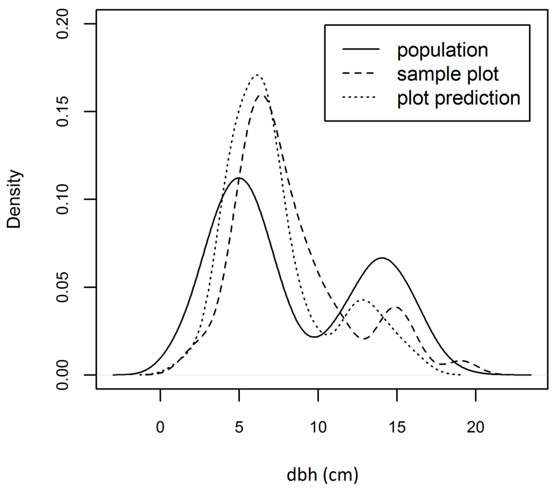
Figure 5.
Effect of bin width on index H values for different combinations of mean and standard deviation values.
Figure 5.
Effect of bin width on index H values for different combinations of mean and standard deviation values.


Table 1.
Summary statistics for plot measurements.
| Statistic | Value |
|---|---|
| measure year | 2009 |
| number of trees | 9210 |
| number of plots | 190 |
| number of species | 63 |
| dominant species | Loblolly P. |
| minimum dbh (cm) | 2.5 |
| mean dbh (cm) | 15.3 |
| median dbh (cm) | 12.2 |
| maximum dbh (cm) | 92.7 |
| standard deviation dbhs (cm) | 11.0 |
| Trees (/ha) | 735.3 |
| BA (m2/ha) | 23.6 |
| Loreys height (m) | 20.1 |
| Volume (m3/ha) | 219.7 |
Trees, BA (basal area per hectare), Lor. (Lorey’s height), and Vol. (total cubic stem volume) are tract level means from plot level calculations, the remaining values were computed from complete tree-lists.
Table 2.
Lidar acquisition parameters.
| Parameters | Value |
|---|---|
| Aircraft Speed (km hr−1) | 220 |
| Flying height (m) | 1430 |
| Nominal density (pulses/m2) | 6 |
| Scan angle (degrees) | ±10 |
| Scan frequency (hz) | 58 |
| Pulse rate (kHz) | 150 |
| Multi-pulse in flight | Enabled |
| Sidelap (percent) | 62.5 |
| Laser beam divergence (mrad @ 1/e) | 0.15 |
| Laser beam diameter at ground (cm) | 22 |
Table 3.
Summary of lidar-derived metrics for plots.
| Variables | Min | Max | Mean | Sd |
|---|---|---|---|---|
| P90 (m) | 3.6 | 36.1 | 20.3 | 6.7 |
| P50 (m) | 2.3 | 32.3 | 15.3 | 6.1 |
| P30 (m) | 1.8 | 30.0 | 12.0 | 5.8 |
| cover(1.50) (%) | 14.5 | 81.9 | 54.1 | 12.8 |
| FWOF (%) | 0.0 | 94.4 | 24.7 | 26.7 |
FWOF refers to Fraction Without Foliage, P30 and P90 refer to 30th and 90th lidar height percentiles, and cover(1.50) refers to the proportion of first returns above 1.50 m. Min: minimum; Max: maximum; Sd: standard deviation.
Table 4.
Index H for k-NN by number of neighbors (k) and distance metric using the three predictor variables P30, P90, and cover(1.50) and responses TPH and Vol. for all species combined.
Table 4.
Index H for k-NN by number of neighbors (k) and distance metric using the three predictor variables P30, P90, and cover(1.50) and responses TPH and Vol. for all species combined.
| k | Euclidean | Mahalanobis | MSN | RF |
|---|---|---|---|---|
| 1 | 0.72 | 0.72 | 0.47 | 0.71 |
| 3 | 0.76 | 0.79 | 0.64 | 0.78 |
| 5 | 0.74 | 0.75 | 0.64 | 0.74 |
| 10 | 0.66 | 0.68 | 0.59 | 0.67 |
| 15 | 0.57 | 0.58 | 0.53 | 0.60 |
| 20 | 0.50 | 0.51 | 0.47 | 0.52 |
MSN, and RF refer to Most Similar Neighbors, and Random Forest respectively.
Table 5.
Sorted index H values for k-NN (k = 3) dbh predictions for selected predictors sets for all species combined with responses TPH and Vol.
Table 5.
Sorted index H values for k-NN (k = 3) dbh predictions for selected predictors sets for all species combined with responses TPH and Vol.
| Set | Predictors | Distance Metric | |||
|---|---|---|---|---|---|
| Euc. | Mah. | MSN | RF | ||
| 1 | P30, P90 | 0.79 | 0.80 | 0.72 | 0.78 |
| 2 | P30, P90, age | 0.78 | 0.80 | 0.72 | 0.79 |
| 3 | P30, P50, P90, FWOF, age | 0.78 | 0.77 | 0.69 | 0.80 |
| 4 | P30, P90, FWOF | 0.79 | 0.78 | 0.71 | 0.79 |
| 5 | P30, P50, P90, age | 0.78 | 0.78 | 0.69 | 0.79 |
| 6 | P30, P90, cover(1.50) | 0.76 | 0.79 | 0.64 | 0.77 |
| 7 | P30, P90, cover(1.50), FWOF | 0.77 | 0.78 | 0.69 | 0.77 |
| 8 | P30, P50, P90, cover(1.50), FWOF, age | 0.76 | 0.76 | 0.68 | 0.78 |
| 9 | P30, P50, P90, cover(1.50), age | 0.76 | 0.76 | 0.69 | 0.77 |
| 10 | P90, age | 0.73 | 0.73 | 0.70 | 0.73 |
| 11 | P90, FWOF | 0.73 | 0.73 | 0.70 | 0.73 |
| 12 | P30, age | 0.72 | 0.72 | 0.62 | 0.73 |
| 13 | P30, FWOF | 0.70 | 0.70 | 0.65 | 0.70 |
| 14 | P90, cover(1.50) | 0.69 | 0.70 | 0.64 | 0.70 |
| 15 | P30, cover(1.50) | 0.65 | 0.66 | 0.46 | 0.66 |
Euc., Mah., MSN, and RF refer to Euclidean, Mahalanobis, Most Similar Neighbors, and Random Forest respectively. FWOF refers to Fraction Without Foliage, P30 and P90 refer to 30th and 90th lidar height percentiles, and cover(1.50) refers to the proportion of first returns above 1.50 m.
Table 6.
Index H values for k-NN (k = 3) dbh predictions for selected predictor and response sets for all species combined.
Table 6.
Index H values for k-NN (k = 3) dbh predictions for selected predictor and response sets for all species combined.
| Response Variables | Predictors | MSN | RF |
|---|---|---|---|
| BA (HS, HW, HW > 23, SW(8–26), SW(26–36), SW > 41) | P30,P90 | 0.81 | 0.79 |
| TPH (HS, HW, SW > 36, SW > 41) | P30,P90 | 0.80 | 0.79 |
| BA (HS, HW, HW > 23, SW(8–26), SW(26–36),SW > 41) | P30,P50,P90,FWOF,age | 0.78 | 0.81 |
| Lor. (HS, HW, SW) | P30,P50,P90,FWOF,age | 0.79 | 0.79 |
| TPH (HS, HW, SW > 36, SW > 41) | P30,P50,P90,FWOF,age | 0.75 | 0.80 |
| BA (HS, HW, SW) | P30,P50,P90,FWOF,age | 0.75 | 0.80 |
| BA, Lor., TPH | P30,P50,P90,FWOF,age | 0.71 | 0.81 |
| BA, Lor., TPH | P30,P90 | 0.71 | 0.79 |
| Lor. (HS, HW, SW) | P30,P90 | 0.70 | 0.78 |
| BA (HS, HW, SW) | P30,P90 | 0.58 | 0.80 |
MSN, and RF refer to Most Similar Neighbors, and Random Forest respectively. Lor. is short for Lorey’s height,. FWOF refers to Fraction Without Foliage, P30 and P90 refer to 30th and 90th lidar height percentiles, and cover(1.50) refers to the proportion of first returns above 1.50 m Items in brackets indicate multiple response variables with different selection criteria including hardwood (HW), softwood (or conifer), and hardwood and softwood (HS) trees; ranges of numbers and greater than symbols indicate selection criteria for dbh values (cm).
Table 7.
Comparison of k-NN (k = 3) density by dbh class with and without stratification for most common species (N = number of plots with species group—it is only by coincidence that both conifers and hardwoods occur on 176 plots each).
Table 7.
Comparison of k-NN (k = 3) density by dbh class with and without stratification for most common species (N = number of plots with species group—it is only by coincidence that both conifers and hardwoods occur on 176 plots each).
| Species | N | Un-Stratified | Stratified | ||
|---|---|---|---|---|---|
| Index H | Dist. Best | Index H | Dist. Best | ||
| all | 190 | 0.81 | RF | 0.78 | RF |
| hardwood | 176 | 0.80 | RF | 0.76 | RF |
| conifer | 176 | 0.71 | RF | 0.64 | RF |
| Loblolly pine | 151 | 0.57 | RF | 0.53 | RF |
| Water oak | 102 | 0.65 | RF | 0.68 | RF |
| Sweetgum | 85 | 0.36 | MSN | 0.39 | MSN |
| Longleaf pine | 79 | 0.54 | RF | 0.47 | RF |
| Black cherry | 71 | 0.45 | MSN | 0.39 | MSN |
| Snag | 66 | 0.41 | RF | 0.38 | RF |
| Laurel oak | 62 | 0.36 | Euc. | 0.30 | Euc. |
| Mockernut hickory | 54 | 0.43 | Euc. | 0.48 | Euc. |
| Blackgum | 54 | 0.37 | RF | 0.52 | RF |
| Post oak | 51 | 0.35 | MSN | 0.43 | MSN |
| Southern red oak | 50 | 0.50 | Euc. | 0.44 | Euc. |
| American Holly | 44 | 0.27 | MSN | 0.41 | MSN |
Euc., Mah., MSN, and RF refer to Euclidean, Mahalanobis, Most Similar Neighbors, and Random Forest respectively. Dist. = none.
Table 8.
Index values (H,I) for k-NN prediction and estimation strategies with k = 3 using the three predictor variables P30, P90, and Cover(1.50) and responses TPH and Vol. for all species combined. We also include the baseline variability (k-NN dist = none) describing plot variability around population dbh density.
| k-NN Dist. | H | I |
|---|---|---|
| none | 0.00 | 0.32 |
| Euc. | 0.76 | 0.16 |
| Mah. | 0.79 | 0.15 |
| MSN | 0.64 | 0.19 |
| RF | 0.78 | 0.15 |
Euc., Mah., MSN, and RF refer to Euclidean, Mahalanobis, Most Similar Neighbors, and Random Forest respectively.
© 2017 by the authors. Licensee MDPI, Basel, Switzerland. This article is an open access article distributed under the terms and conditions of the Creative Commons Attribution (CC BY) license (http://creativecommons.org/licenses/by/4.0/).
Share and Cite
MDPI and ACS Style
Strunk, J.L.; Gould, P.J.; Packalen, P.; Poudel, K.P.; Andersen, H.-E.; Temesgen, H. An Examination of Diameter Density Prediction with k-NN and Airborne Lidar. Forests 2017, 8, 444. https://doi.org/10.3390/f8110444
AMA Style
Strunk JL, Gould PJ, Packalen P, Poudel KP, Andersen H-E, Temesgen H. An Examination of Diameter Density Prediction with k-NN and Airborne Lidar. Forests. 2017; 8(11):444. https://doi.org/10.3390/f8110444
Chicago/Turabian StyleStrunk, Jacob L., Peter J. Gould, Petteri Packalen, Krishna P. Poudel, Hans-Erik Andersen, and Hailemariam Temesgen. 2017. "An Examination of Diameter Density Prediction with k-NN and Airborne Lidar" Forests 8, no. 11: 444. https://doi.org/10.3390/f8110444
Note that from the first issue of 2016, this journal uses article numbers instead of page numbers. See further details here.