Using Linear Mixed-Effects Models with Quantile Regression to Simulate the Crown Profile of Planted Pinus sylvestris var. Mongolica Trees


Department of Forest Management, School of Forestry, Northeast Forestry University, Harbin 150040, China
*
Author to whom correspondence should be addressed.
Forests 2017, 8(11), 446; https://doi.org/10.3390/f8110446
Submission received: 17 October 2017
/
Revised: 9 November 2017
/
Accepted: 14 November 2017
/
Published: 17 November 2017
(This article belongs to the Special Issue Successional Dynamics of Forest Structure and Function)
Abstract
:Crown profile is mostly related to the competition of individual trees in the stands, light interception, growth, and yield of trees. A total of 76 sample trees with a total number of 889 whorls and 3658 live branches were used to develop the outer crown profile model of the planted Pinus sylvestris var. mongolica trees in Heilongjiang Province, China. The power-exponential equation, modified Kozak equation, and simple polynomial equation were used and the model which showed the best performance was used as the basic model. The dummy variable approach was used to analyze the effect of stand age and stand density on the crown profile. Quantile regression for linear mixed-effects model, where the correlations between the series measurements on the same subject were considered, was used to model the outer crown profile. The results indicated that the power-exponential equation had the smallest error and was used as the basic model. Based on the dummy variable approach, stand age and stand density showed significant effects on the crown profile on the whole. Thus, they were directly included into the linear form of the power-exponential equation by a natural logarithm transformation to develop the quantile regression for the linear mixed-effects model. The 0.95th quantile regression model performed best in modeling the outer crown profile when compared to other quantiles. The prediction accuracy of the 0.95th quantile regression model by adding the random effects increased when compared to the quantile regression without random effect. The quantile regression for the linear mixed-effects model also showed an excellent performance in the largest crown radius prediction when compared to the quantile regression model. From suppressed trees to dominant trees, the crown radius increased, with tree size increasing for the same stand age and stand density increases. The crown radius of the suppressed trees from 21 to 40 year stands was the largest and the smallest was from older (>40 years) stands. The crown radius for both the intermediate and dominant trees from 21 to 40 year stands were similar and were larger than the younger (10–20 years) stands. The crown radius increased with tree size when the stand variables were constant. Furthermore, the crown radius increased with the increase of stand age, decreased with increasing stand density, and decreased with increased ratio of tree height to diameter at the breast height (HD) for trees with the same tree variables. Stand density had a weaker effect on the crown profile when compared to the HD. The growth rate of the crown radius of planted Pinus sylvestris var. mongolica trees increased with increasing stand age, and decreased with decreasing stand density. The growth rate of the crown radius decreased with increasing HD.
1. Introduction
The crown profile, which is a useful predictor for crown size, has attracted the most attention as it exhibits a close relationship between species diversity and ecosystem stability [1,2,3]. The crown profile of a tree is generally characterized by simple regular geometrical shapes [4,5] or mathematical equations [6,7,8,9]. However, the mathematical equations are thought to be much more flexible when delineating the plastic crown profile when compared to regular geometrical shapes [9,10]. To describe the outer contour of a tree crown, the approach most commonly used to predict the crown radius at any position is the use of tree variables as the predictors. Diameter at the breast height (DBH), crown length (CL), crown ratio (CR), the largest crown radius (LCR) and other variables on the tree level have been the most commonly used in crown profile model construction [6,9,11]. The impact of the environment and stand variables also play essential roles in the crown profile model. Dong et al. [12] developed a crown profile model for Chinese fir (Cunninghamia lanceolata) for three groups of site index and the differences of crown profile between site indexes were found. Guo et al. [13] studied the crown profile from different age groups for the Chinese fir (Cunninghamia lanceolata) and developed a crown profile model for each age group. Stand density, another important stand variable, has also been considered in the crown profile model. However, it has seldom been directly included in the crown profile model as the predicted crown radius might expand unrealistically in response to forest management activities [14]. Tree variables, such as DBH, tree height, the height to the base of the live foliage, and the ratio of tree height to DBH, are the results of the tree’s response to environmental factors [9]. As a result, much research has used tree variables to reflect the effect of stand density on crown profile indirectly [9,14,15]. However, the effect of stand density on the crown profile is still unclear. Until now, most analysis has still been based on classic regression that conventionally estimates the conditional means of the response variable within the least-squares framework [16,17]. Thus, the fitted outer crown curve has only been confined to describe the central trend of the data. Classic regression only works well when the regression assumptions are met: the error term of the model should follow a normal distribution, and the variance of the error term should follow homoscedasticity and independence between variables [18]. Therefore, the fitted crown curve based on classic regression is not really the outer crown profile.
Quantile regression, introduced by Koenker and Bassett [19,20], provides a comprehensive approach for estimating multiple conditional quantile functions by applying a specific quantile parameter without imposing any distribution assumption on the error term [16]. In addition, quantile regression possesses other specific advantages, i.e., robustness to the distribution assumption, monotone equivariance characteristics, and insensitivity to the outliers without the necessity of subjectively selecting data [16,20,21,22]. Due to the flexible characteristic of quantile regression, it has been widely used in various research areas such as ecology [23,24], education policy [25], medicine [26], economic research [27,28], and forest resource management [29]. Zhang et al. [22] used quantile regression to model the self-thinning line for a Pinus strobus L. plantation and the results showed that quantile regression performed well in modeling the maximum density line. Mehtätalo et al. [30] predicted diameter distribution by using quantile regression, as have other studies found in the research of Ducey and Knapp, Bohora and Cao, and Gao et al. [31,32,33]. The combination of quantile regression and Bayesian models has also been used in a study with count data [34]. Additionally, nonlinear quantile regression has already been used to enable more accurate depictions of the outer crown profiles of individual trees by selecting the specific quantile (e.g., quantile = 0.90) [11]. However, the data used in these studies had a nested or clustered structure and the correlation between the measurements was not clearly explained in the quantile regression model.
Mixed-effects models that include fixed effects to account for covariate effects and random effects to explain heterogeneity between the subjects provides efficient analysis on hierarchical or nested data [35]. Quantile regression has also been extended to the linear mixed-effects model [36,37]. The parameters of quantile regression for the linear mixed-effects model (qrLMM) achieve an unbiased estimation due to the fact that the correlation of the measurements from the same subjects are adequately accounted for [36]. Liu and Bottai [38] studied the parameter estimation of the qrLMM based on Monte Carlo simulations for the fixed parameters of the model given the assumption that no correlation existed between the random effects parameters. Chen et al. [39] proposed a marginally-conditional quantile regression approach to deal with the longitudinal dataset by including the random observing times, and the consistency and asymptotic normality for the estimators were developed. Other productive studies were found in Marino and Farcomeni, and Li et al. [40,41]. Galarza and Lachos [37] used the stochastic approximation of the expectation-maximization (EM) algorithm to derive the maximum likelihood estimates of the fixed effects and variance component of the quantile regression for the linear mixed-effects model, and this method was constructively implemented by the R (Vienna, Austria) package qrLMM [37,42,43].
To the best of our knowledge, the mixed-effects model incorporating quantile regression has not been used in crown profile descriptions until now. Our study developed a new crown profile model based on the power-exponential equation to model the crown profile of planted Pinus sylvestris var. mongolica trees in Heilongjiang Province, Northeast China. In addition, a modified Kozak equation and a simple polynomial equation were also compared and the equation that performed best was used for further analysis. The dummy variable approach was used to analyze the effect of age and stand density on the crown profile. A specific quantile describing the crown profile was further selected. The quantile regression for the linear mixed-effects model (qrLMM) including the random effects on the tree level was further used to predict the crown radius, and was compared to the crown radius predicted by the quantile regression model without the random effects. In addition, the accuracy of the largest crown radius prediction was also compared between the qrLMM and quantile regression model without random effects. The purpose of the study was to introduce the application of the new approach, quantile regression for linear mixed-effects model, into crown profile modeling. We further proposed the analysis of crown profiles for different tree statuses (dominant tree, intermediate tree, and suppressed tree) between different stand ages and density, and the effect of stand age and stand density on the crown profile of planted Pinus sylvestris var. mongolica.
2. Materials and Methods
2.1. Study Area and Data Collection
The study area is located in the Mengjiagang forest farm (130°32′42″–130°52′36″ E, 46°20′16″–46°30′50″ N) and Hengtou Mountain forest farm (130°28′29″–130°44′09″ E, 46°34′40″–46°34′40″ N) in Heilongjiang Province, Northeast China. The main terrain from the three forest farms consists of low mountains and hills with gentle slopes. The Mengjiagang forest farm is located to the west of Wanda Mountain. The average elevation of this area is 250 m. The annual average temperature is 2.7 °C, and annual average precipitation is 550 mm. The frost-free period is about 120 days per year. The Hengtou Mountain forest farm also belongs to the Wanda Mountains where the average elevation is 350 mm. The average annual temperature is 2.5 °C, and the annual average precipitation is 460 mm. The frost-free period is about 130 days per year.
2.2. Data Collection and Analysis
A total of 15 permanent sample plots 20 m × 30 m in size were established in the study area from 2002 to 2006. All trees in the plots were measured for diameter at breast height (DBH, cm), which was defined as 1.3 m above ground level; total tree height (HT, m) using a Vertex IV Ultrasonic Hypsometer (Haglöf, Sweden); and crown width (CW, m). All trees in the plots were divided into five intervals with the equivalent cumulative basal area for each interval with one average tree from each interval selected as the sample tree. Thus, a total of five trees were selected in each plot. Additionally, another average tree was selected from Plot 15 (Table 1). As a result, a total of 76 trees with healthy crowns were selected. Forty-six trees were selected from the Mengjiagang forest farm during the period of 2005–2006, and 30 trees were selected from the Hengtou Mountain forest farm in 2004. The attributes of the 15 sample plots are shown in Table 1.
DBH and CW were measured for all the sample trees before they were felled. A straight line was used to determine the azimuth of all the branches, and was marked from the ground to the height of the DBH on the northern side of the trunk and extended to the tree tip after the tree was felled. When the sample tree was felled, the total tree height was re-measured and the height to the first live branch of the whorl containing at least three branches (HBLC, m) was measured. In our study, the lowest whorl containing at least three branches was defined as the crown base. Thus, crown length (CL, m) was defined as CL = HT – HBLC. The trunk was divided by one-meter sections from the base of the trunk to the tree tip, and the smaller than one meter section remaining was recognized as the tree tip. Branch diameter (BD, mm), branch angle (VA, °), branch chord length (BC, cm), and absolute depth into the crown from the tree tip down to the branch basis (L, cm) were measured sequentially for all the branches from a specific section from the tree tip down to the crown base after the section was placed upright on the ground. For all branches, the branch radius (BR) was calculated as the product of its branch chord length and the sine of the branch angle, and the corresponding absolute distance into the crown (DINC, m) was the difference between the length from the tree tip to the branch base and the projection onto the trunk of the branches based on the trigonometric relationship. Relative distance into the crown radius of interest (RDINC) was defined as RDINC = DINC/CL. In our study, a total of 3658 branches were measured. The statistics of the sample trees and branches are listed in Table 2, and the branch variables are described in Figure 1. The branch with the largest crown radius from each whorl of all the sample trees was selected and was recognized as the whorl radius (WR). Thus, a total of 889 of the largest branches were selected.
2.3. Model Selection for the Crown Profile
The power-exponential equation is a special function in advanced mathematics. However, this function has not been used in the study of crown profile models. We analyzed the curve of this equation and changed the symbol of the parameter of the equation to make the curve reasonable to describe the outer crown profile of the planted Pinus sylvestris var. mongolica trees. The power-exponential equation is shown as Equation (1):
where WR is the whorl radius of the crown based on the largest branches selected from each whorl; RDINC is the relative distance into the crown; and a1, a2, and a3 are the parameters to be estimated. To make the curve reasonable in describing the outer crown profile, the parameters should be restricted as a1 > 0, a2 > 0, and a3 < 0. By analyzing the relationship between the parameters and tree variables, DBH, CR, and HD were at last introduced into the equation and the model is finally defined as Equation (2):
where a1–a5 are the model parameters to be estimated. DBH is the diameter at breast height, CR is the crown ratio, and HD is the ratio of tree height to DBH.
In addition, two other equations, the modified Kozak and simple polynomial equations (which have been used by other studies), were also used and compared in our study. The Kozak model was first introduced into the study of stem profile description, and was then modified to model the outer crown profile [11,15]. The modified Kozak equation is shown as Equation (3):
where a1–a6 are the model parameters.
The simple polynomial equation was also used and compared in the present study, and is shown as Equation (4):
where a1–a4 are the model parameters to be estimated.
Equations (2)–(4) were fitted by using all of the 889 largest branches, and Ra2, root mean square error (RMSE), and Akaike information criterion (AIC) were used to compare the goodness-of-fit of the three basic models. The mean error and mean absolute error for the upper crown, shade crown, and the total tree were calculated. The model with the largest Ra2, the smallest RMSE and AIC, the smallest mean error and mean absolute error was selected as the best model to develop the outer crown profile model.
The dummy variable approach based on the best equation selected was used to analyze the effects of stand age and stand density on the crown profile, respectively. All trees were divided into four groups (<20, 21–30, 31–40, 41–50) based on the stand age and four groups (<1000, 1001–2000, 2001–3000, >3000) based on the stand density.
2.4. Quantile Regression for the Mixed-Effects Outer Crown Profile Model
The outer or outer contour of the exterior edges of the crown was used to characterize the crown profile of a standing tree [11]. Based on the selected equation that best modelled the crown profile, a specific quantile to model the outer crown profile was taken following the study of Gao et al. [11]. The quantile curves were fitted using all the branches by a series of quantiles, from 0.50 to 0.95 with an interval of 0.05 plus the value of 0.99. Three fixed effects (marginal) models with the same equation form were fitted to the entire dataset (the first marginal model), about half of the dataset (the second marginal model) after removing the non-positive residuals of the first marginal model, and about a quarter of the dataset (the third marginal model) of the whorl radius data after removing the non-positive residuals of the second marginal model. The quantile curve that was mostly adjacent to the third marginal model was selected to describe the outer contour of the exterior edges of the crown. This detailed information could be found in the study of Gao et al. [11].
The branches used to model the crown profile were nested into the tree and the correlation relationship between the branches needed to be explained. The quantile regression for linear mixed-effects models where the correlation between the branches within the individual trees was considered by including the random effects were introduced into the outer crown profile model. The Stochastic-Approximation of the EM Algorithm (SAEM) is used to perform the quantile regression for linear mixed-effects models. The d, p, q and r functions for the Asymmetric Laplace Distribution are defined in this model. To explain the hierarchical representation of the Asymmetric Laplace Distribution, exact maximum likelihood estimates of the fixed-effects and variance components is derived based on SAEM [42]. The general linear mixed-effects model is defined as Equation (5):
where yij is the jth observation from the ith subject; is design matrix with the dimension of N × k; β is the fixed effects parameters with the dimension of k × 1; zij is the design matrix with the dimension of q × 1; and bi are the random effects with the dimension of q × 1. Thus, the qth quantile regression for linear mixed-effects model is written as Equation (6):
Akaike information criteria (AIC), Bayesian information criteria (BIC), log-likelihood (LL), and Hannan–Quinn information criterion (HQC) were used to evaluate the performance of the model. The model that had the smallest AIC, BIC, HQC, and the largest LL performed best. The functions are shown as Equations (7)–(9):
where k is the number of parameters, and n is the number of observations. All of the analyses in our study were based on R software [43]. The qrLMM package was used to estimate the parameters of quantile regression for linear mixed-effects models [42]. The generally positive matrix was used to explain the variance-covariance matrix for the random effects parameters for the specific quantile. Statistical indices used to evaluate the marginal models and quantile regression models were R2, Var(εp), [E(εp)]2, predicted mean error (MEP), and predicted mean absolute error (MAEP); and the function can be found in Gao et al. [11]. Based on the results of the dummy variable approach, stand age and stand density were introduced into the quantile regression for the mixed-effects outer crown profile model to analyze the effect of stand variables on the crown profile.
3. Results
3.1. Best Model Selection for the Crown Profile Model
Based on the results of the goodness-of-fit statistics for the three basic models (Table 3), the power-exponential equation (Equation (2)) showed the best performance with an Ra2 of 0.79, RMSE of 0.3544 m, and AIC of 762. Additionally, Equations (2)–(4) were further used to predict the crown radius for the total tree, upper crown, and shade crown. For the total tree, the power-exponential equation and modified Kozak equation produced an equivalent mean error, and the simple polynomial equation produced a relatively larger mean error. As for the light crown, the crown radius was overestimated by all three equations. The mean error for the power-exponential equation was 0.0224 m, which was the largest compared to the two other equations, but still lower than 0.03 m. For the shade crown, all three equations underestimated the crown radius. The modified Kozak equation had the smallest mean error, and the power-exponential equation was slightly larger, while the simple polynomial equation was the largest. In comparison, the power-exponential equation produced the smallest mean absolute error for the total tree, upper crown, and lower crown, and the simple polynomial equation was the largest. Due to the fact that the error produced by the individual trees was mainly derived from the shade crown, the comparison between the shade crowns was used as the criteria to select the best model. Thus, the power-exponential equation was selected as the best equation to model the outer crown profile for the planted Pinus sylvestris var. mongolica trees. The parameters in Equation (2) were restricted as a1 > 0, a2 > 0, and a3 < 0 so that the curve could approach the true shape of the crown. By reparametrization, > 0, (a2 + a3)·CR > 0, and (a4 + a5)·HD < 0, which meets the requirement of the symbol of the parameters.
The dummy variable approach was used to analyze the effect of stand age and stand density on the crown profile, respectively. Based on Equation (2), all parameters were used as the dummy variable. The model with a3 as the dummy variable for both stand age and stand density showed the best performance. The models are shown as Equations (10) and (11).
where A1, A2, A3, and A4 indicate the stand age of <20, 21–30, 31–40, 41–50, and SD1, SD2, SD3, and SD4 indicate stand density of <1000, 1001–2000, 2001–3000, and >3000, respectively. The estimates for the parameters are shown in Table 4.
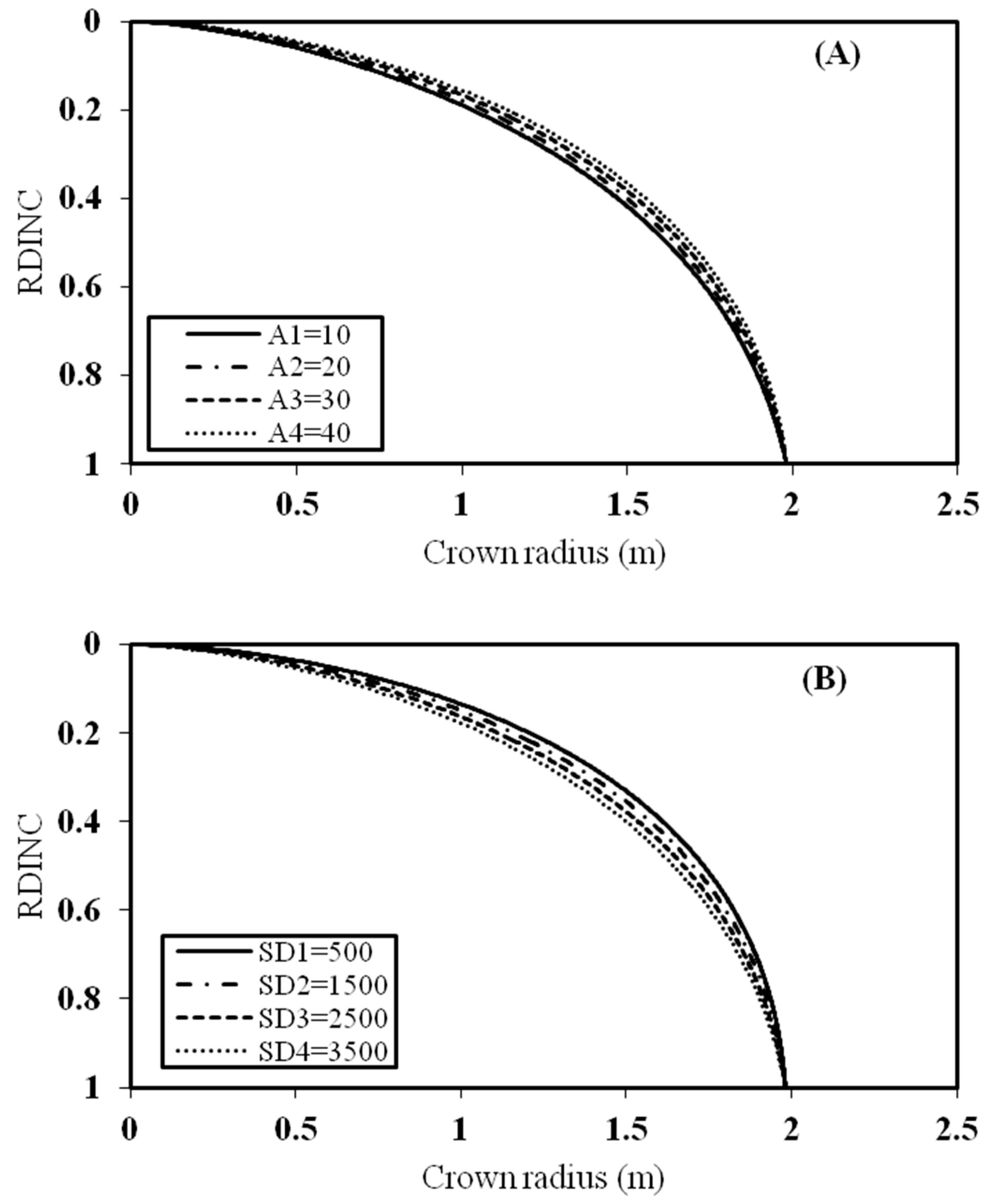
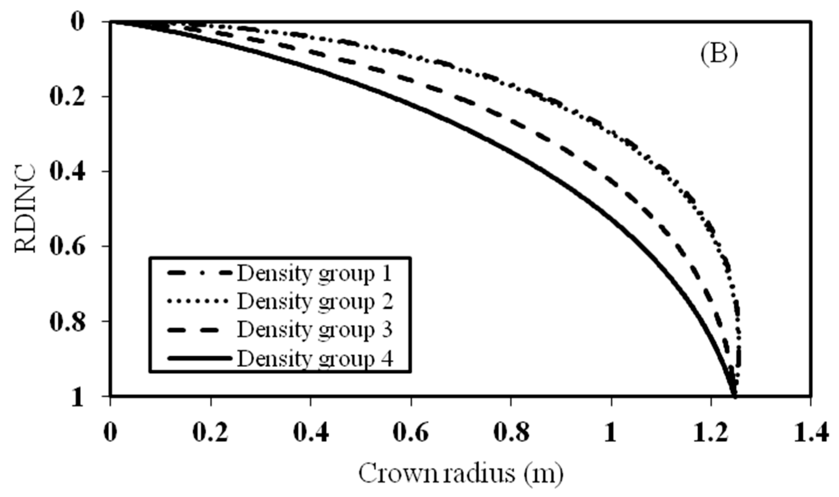
One tree was randomly selected to reflect the effect of stand age and stand density on the crown profile (Figure 2). Figure 2A shows that the tree with a stand age of between 41 and 60 years (Age group 4) had the largest crown radius, and the stand age of lower than 20 years (Age group 1) had the smallest crown radius. The predicted crown radius of stand age between 21 and 30 years (Age group 2) was almost equal to 31–40 years (Age group 3) due to the almost equivalent estimates of parameter a6 and a7 (Table 4). On the whole, this indicated that the crown radius for the tree with the same size increased with the increasing of age. As for stand density (Figure 2B), the predicted crown radius of the tree from a stand density of larger than 3000 trees ha−1 (Density group 4) had the smallest crown radius, followed by the density of between 2000 and 3000 trees ha−1 (Density group 3). The tree from the stand density between 1000 and 2000 trees ha−1 (Density group 2) and the stand density of lower than 1000 trees ha−1 (Density group 1) had the largest crown radius. However, the crown radius of the two groups was almost equivalent.
3.2. Quantile Regression for the Linear Mixed-Effects Crown Profile Model
The quantile regression model was used to describe the crown profile of the individual tree. The branch radius of all the branches was substituted to the whorl radius to fit the quantile regression model. Due to the fact that the linear model was much easier to fit compared to the nonlinear model, the natural logarithm of the two sides of Equation (2) was used in this study. Based on the analysis by the dummy variable approach, stand age and stand density affected the crown profile of individual tree. Thus, stand age and stand density were finally included in the model shown as Equation (12).
where ln is the natural logarithm for the branch variables; BR is the branch radius for all the branches; A is the stand age; SD is the stand density; and b1–b2, b31–b33, b4–b5 are model parameters.
To facilitate the fitted curves of the crown profile approximating the outer contour of the exterior edge of the crown, linear quantile regression based on Equation (12) with the quantile from 0.50 to 0.95 with an interval of 0.05, plus 0.99, was used to develop the crown profile model. Following the method of selecting a quantile to model the outer crown profile from Gao et al. [11], the 0.95th quantile almost performed as well as the third marginal model using approximately one quarter of all branches. The 0.90th and 0.99th quantile curves were all inferior to the 0.95th quantile and the third marginal model (Table 5). The mean error and the mean absolute error in Table 4 also indicated that the 0.90th and 0.99th quantile curves were inferior to the 0.95th quantile curve. Thus, the 0.95 quantile curve was mostly suitable to describe the outer crown profile for the planted Pinus sylvestris var. mongolica trees.
In our study, all branches from the sample trees of the planted Pinus sylvestris var. mongolica trees were measured, which facilitated the use of the quantile regression model by including the random effects, and Equation (12) was used as the basic equation. For Equation (12), b1, b2 were assumed to be the random effects on the individual tree level. The following is the process of calculating the fixed effects parameter and variance-covariance structure for the random effects of qrLMM with the same equation form Equation (13):
where fixed[1]–fixed[7] are the fixed parameters. Thus, the fixed effects of the quantile regression for linear mixed-effects model were lnDBH, lnRDINC, CR·lnRDINC, A·CR·lnRDINC, SD·CR·lnRDINC, RDINC, and HD·RDINC, and the random effects of the qrLMM were lnDBH and lnRDINC.
Based on the 0.95th linear quantile regression model, all possible expansions of only one, two, and three parameters were considered as random effects, and all the models achieved convergence. The models with more than three random effects did not converge and the performance of the model did not improve significantly. Therefore, we compared the mixed-effects models with only one, two, and three random-effects and the results are in Table 6. The qrLMM with b1, b31, and b5 as the random effects achieved the smallest AIC, BIC, and HQ, and the largest logLike and was selected as the best model. Compared to the 0.95th linear quantile regression model, the R2 of the qrLMM, considering b1, b31, and b5 as the random effects parameters, increased and [E(εp)]2 decreased (Table 5). The mean error and mean absolute error of qrLMM were also decreased when compared to the linear quantile regression (Table 5). Therefore, the precision and predicted ability of quantile regression for the linear mixed-effects model was improved when compared to the quantile regression model. The estimates for the parameters and variance-covariance structure are listed in Table 7 and all parameters were stable.
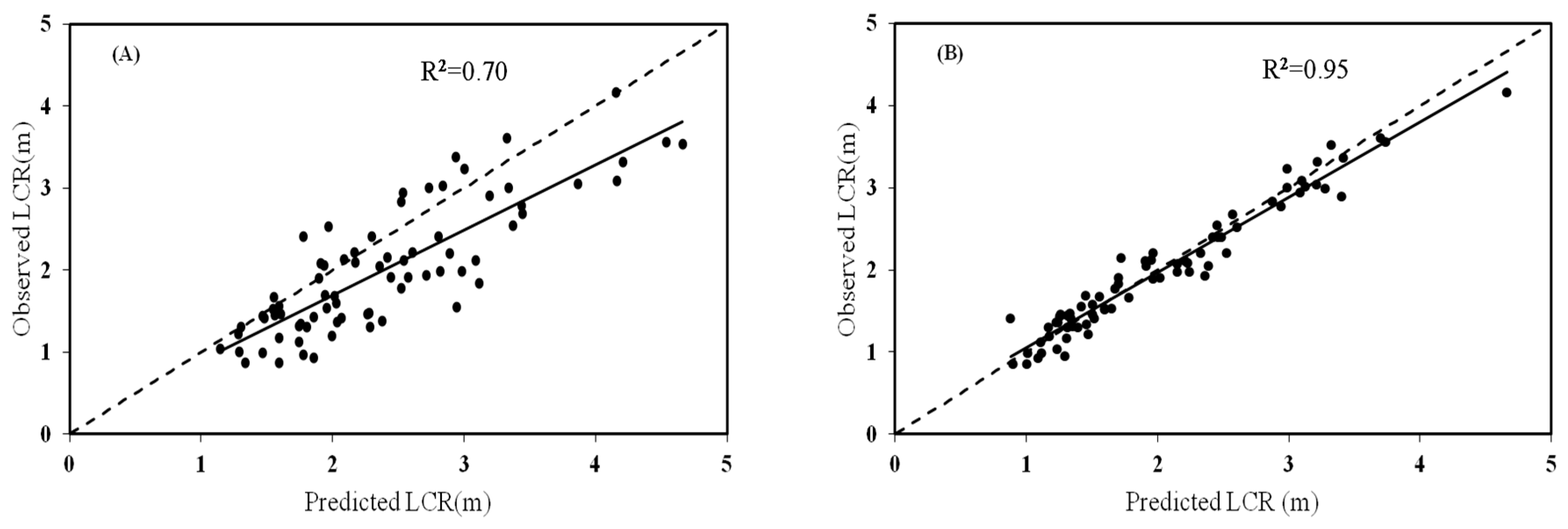
The largest crown radius of all sample trees was calculated with the 0.95th linear quantile regression model and the 0.95th quantile regression for linear mixed-effects model with random effects of b1, b31, and b5 at the tree level, respectively. The predicted largest crown radius by linear quantile regression and qrLMM were plotted against the observed values as shown in Figure 3. It was well documented that the largest crown radius for most trees was overestimated by the linear quantile regression model, while this situation was improved for the qrLMM. The predicted largest crown radius by qrLMM against the observed value was almost distributed around the two sides of y = x. The predicted largest crown radius by quantile regression and qrLMM was also regressed with the observed largest crown radius, respectively. The R2 for the linear quantile regression model was 0.70, and the quantile regression for the linear mixed-effects model was 0.95 (Figure 3). Thus, the prediction for the largest crown radius by qrLMM was improved by adding the random effects into the quantile regression.
Three trees (one dominant tree, one intermediate tree, and one suppressed tree) with different sizes from three plots with different stand age and stand density were selected and the fitted outer crown profile curves against the observed crown radius of the three trees are shown in Figure 4. Ultimately, the quantile regression for the linear mixed-effects model was powerful and suitable in modeling the outer crown profile. For trees from the same plot with the same stand age and stand density, the crown radius increased from the suppressed tree to dominant tree (Figure 4(A1–A3); Figure 4(B1–B3); and Figure 4(C1–C3)). The suppressed tree from the stand age of 33 years (B1) possessed the largest crown and the suppressed tree from the stand age of 44 years (C1) appeared to possess the smallest. The intermediate tree from the stand age of 33 years (B2) and the stand age of 44 years (C2) had a similar crown in size and was larger than the intermediate tree from the stand age of 20 years (A2). The regularity of the crown profile for the dominant tree with the stand age from 20 to 44 years was the same as the intermediate trees.
3.3. Effect of Stand Age and Stand Density on the Crown Profile
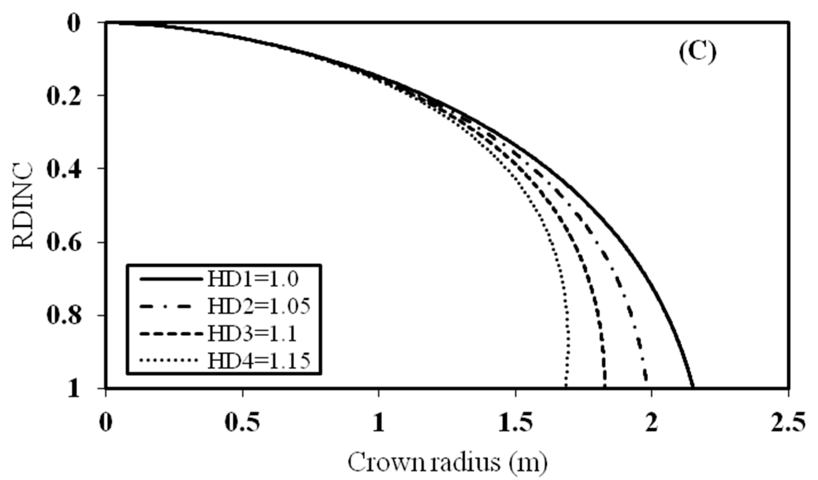
One medium sized tree was selected to analyze the effect of stand age, and stand density on the crown profile. HD is another variable that reflects the effect of stand density on the crown profile, so it was also analyzed (Figure 5). In Figure 5A, the effect of stand age on the crown profile was analyzed while the other variables were kept constant. This indicated that the crown radius of the tree increased with increasing stand age. The RDINC of the tree was divided by 100 intervals and the difference of each interval between A1 and A2, A2 and A3, A3 and A4 was calculated. The sum of the difference for the 100 intervals of A1 and A2, A2 and A3, A3 and A4 was calculated. The sum of the difference of A1 to A2 was 20.38 m, 20.93 m for A2 to A3, and 21.51 m for A3 to A4. Thus, the growth rate of the crown radius of planted Pinus sylvestris var. mongolica trees from A1 to A4 within the stand age of between 12 and 46 years increased with increasing stand age. For Figure 5B, the crown radius decreased with increasing stand density. Similar to the analysis method used for stand age, the sum of difference of SD2 to SD1 was 26.63 m, 27.55 m for SD3 to SD2, and 28.53 m for SD4 to SD3. This showed that the growth rate of the crown radius decreased with a decrease in stand density. In contrast to stand age and stand density, the tree variable HD showed a relatively larger effect on the crown profile (Figure 5C). HD mainly affected the crown profile of the lower part of the crown. The crown radius decreased with increasing HD. The sum of difference of HD2 to HD1 was 74.79 m, 70.63 m for HD3 to HD2, and 66.73 m to HD4 to HD3. The growth rate of the crown radius decreased with increasing HD.
4. Discussion
The crown profile model that depicts the outer contour of the exterior edges of the crown has played an essential role in the growth and yield models of individual trees and stands [6,7,44,45]. In this study, we developed a new crown profile model and the effect of stand age and stand density on the crown profile was analyzed. The incorporation of quantile regression into the linear mixed-effect model increased the accuracy of the crown profile model.
The model selection process is important in crown profile modeling. The feature of the tree species was the main reason to determine the shape of crown. This meant that an equation mostly suitable to describe other tree species may not have shown a good performance in our study. Thus, we listed the modified Kozak equation that has recently been demonstrated as flexible, and showed good performance in crown profile modeling [11,15]. Based on the exploratory analysis of the field measurement data on the screen tree by tree, a simple polynomial shape for most of the trees was detected. The reason for this was that the crown base was defined as the whorl containing at least three branches in our study and no inflection points were detected in the crown profile for some of the trees. In the study of Gao et al. [11,15], the lowest whorl that had at least one live branch was defined as the crown base. Therefore, we also used the simple polynomial equation, similar to the study of Crecente-Campo et al. [9], Dong et al. [12], and Sotocervantes et al. [46]. The power-exponential equation has yet to be used in crown profile modeling. By changing the symbol of the parameters of this equation, it conformed to the shape of the crown. This was the reason why this equation was used to depict the crown profile of the planted Pinus sylvestris var. mongolica trees. In comparison, the power-exponential equation had the lowest mean absolute error for the total tree, upper crown, and shade crown. Thus, it was the most desirable equation to model the planted Pinus sylvestris var. mongolica trees in our study.
We measured all the branches of the sample trees, which made it possible to use the quantile regression approach by considering all the information of the branches. It has been previously demonstrated that quantile regression models showed stable characteristics at, or close to, the median part of the data cloud [20,47]. By including the random effects parameters in the quantile regression model, the dependence between the series measurements for the branches within the same tree was adequately described (Table 5). The outer crown profile is relatively difficult to quantify, to some extent due to the characteristics of the flexibility of the crown. Thus, the crown shape fitted by the largest branch selected from each whorl or stem section was easily affected by the abnormal largest branch. To avoid the situation of subjective data selection, Gao et al. [11] used quantile regression to develop the outer crown profile curve. We further used the quantile regression for the linear mixed-effects model including the random effects to account for the within-tree dependence of branches. This was the main reason why we promoted this powerful approach in the outer crown profile model development. Following the approach of Gao et al. [11], which was to select the quantile to describe the outer crown profile, we selected the 0.95th quantile to model the outer crown profile.
The largest crown radius is an important crown variable as it is useful to estimate the canopy cover of the forest stand [14]. Fu et al. [48,49] developed the crown width model using a nonlinear mixed-effects approach and developed a system of crown width models focusing on the additivity and inherent correlation. Sharma et al. [50] also developed a crown width model by including the explicit and non-explicit competition measures. Their models showed excellent performance in crown width prediction. The outer crown profile models developed in our study also showed good performance in the largest crown radius by the quantile regression with an R2 of 0.70. Furthermore, the R2 of the largest crown radius increased to 0.95 by including the random effects into the quantile regression model. Thus, the quantile regression for the linear mixed-effects model for the outer crown profile showed good performance in both describing the crown shape and largest crown radius prediction. Thus, the largest crown radius is very useful in canopy closure estimation with higher precision. Besides, it is also helpful to study the competition between the subject trees and neighbor trees. The biological diversity and the habitat of the wildlife in the stand are also closely related to the crown structure and the crown layer. It indicated that the crown profile model is not only useful in the individual tree growth and yield model, but also very useful in the biological research area. This is why we used the quantile regression for linear mixed-effects models to increase the prediction precision for the largest crown radius.
The effect of stand variables on the crown profile has been assessed mainly by including only tree variables [9,10,11,51] as including the stand variables in the model may lead to unreasonable results [52]. Gao et al. [15] demonstrated that variations of the crown profiles for Larix olgensis trees existed between tree statuses (dominant, intermediate, and suppressed tree). In our study, we further demonstrated that variations also exist in the crown profile of the tree with the same tree status from different stand ages. For trees from younger stands, most of them had the vigorous ability to obtain more sunlight to grow into the upper layer of the forest canopy. With the development of the stands, the competition turns much fiercer, and the dominant trees possess the upper layer of the forest canopy and occupy the absolute advantages compared to the suppressed trees. Thus, the crowns of dominant trees grow much larger and the suppressed trees become much smaller. This is the reason why the crown radius of the suppressed trees from the stand age of 44 years was smaller than 33 years; however, the differences for the intermediate trees between 33 years and 44 years were not significant. This could be because the intermediate trees from 33 years had stronger tree vigor than those from 44 years as the inhibitory effects from the dominant trees are much stronger compared to the stand of 33 years.
Attocchi and Skovsgaard [53] predicted that the crown radius of Quercus robur L. was related to stem size, stand density, and site productivity, and indicated that the thinning grade and site productivity all had an influence on the crown radius which determined the crown shape of the tree. Bechtold [51,54] found that stand density would affect the largest crown width prediction. However, Ritchie and Hann [14] thought that stand density was inappropriate to incorporate into the crown profile model given that the predicted crown radius might expand unrealistically in response to forest management activities. We used the dummy variable approach to analyze the effect of stand age and stand density on the crown profile by using the 889 largest branches. Figure 2 indicated that the stand age and stand density had a significant effect on the crown profile on the whole. Therefore, we added the stand age and stand density into the quantile regression for linear mixed-effects model directly with linear form to describe the outer crown profile of the planted Pinus sylvestris var. mongolica, and reasonable results were achieved. In Equations (10) and (11), parameter a3, used as the dummy variable for both stand age and stand density, showed the best performance. Therefore, we constructed a crown profile model including stand age and stand density as Equation (12). The crown radius of the trees with the same size increased with increasing stand age and our results conformed to the study of Baldwin et al. [6]. The reason is that the trees occupy a relatively larger space to grow in a larger age group than in a lower age group. The stand age and stand density also provide a biological explanation about the effects on the crown profile. Due to the stand environment variations and the differences of competition level between the sample trees, the trees with the same stand age might show different crown profile. It could explain the growth history of the individual trees and it could provide effective measurement for forest management. The trees with the same age that achieved different crown profiles also showed the biological variations between the individual trees. The trees will grow into the upper layer or occupy the released space due to the change of the stand density. Thus, the trees with the same stand age but different growth environment might show different crown profiles. We also analyzed the effect of both stand density and HD on the crown profile. Stand density had a weaker effect on the crown profile when compared to HD. The possible reason is that the range of stand density is narrow within each group so variations could not be reflected. Another reason might be that the change of crown profile lags when responding to the change of stand density. Thus, we propose that the method of using HD to substitute the effect of stand density is encouraging if the data of stand density is missing.
5. Conclusions
In our study, the quantile regression for a linear mixed-effects model was applied to crown profile modeling. The power-exponential equation was used as the basic equation to develop the crown profile model. The 0.95th quantile was suitable to describe the outer crown profile with the dependence of measurement for the branches from the same tree reasonably explained. By including the random effects into the quantile regression model, the prediction accuracy of the crown profile model and the largest crown radius was improved when compared to the quantile regression model. The crown radius of trees with the same stand age and stand density increased from suppressed trees to dominant trees. The crown radius of the suppressed trees from the stand age of 33 years was the largest and 44 years was the smallest. The crown radius for both the intermediate and dominant trees from the stand age of 33 years and 44 years were similar and the stand age was larger than 20 years. Both stand age and stand density had important effects on the crown profile. The crown radius of the individual tree increased with increasing tree size under the same stand condition. The crown radius increases with the increase of stand age and decreases with the increase of stand density and HD for the trees with the same tree sizes.
Acknowledgments
This research was financially supported by the National Natural Science Foundation of China (31570626). The authors warmly thank Bi for his help in quantile regression and Galarza for his help in parameter estimation of quantile regression for linear mixed-effects model. The authors also thank the teachers and students of the Department of Forest Management, Northeast Forestry University (NEFU), China, who provided and collected the data for this study.
Author Contributions
Yunxia Sun undertook data analysis, and wrote most of the paper. Huilin Gao helped with the data analysis and modified the paper. Fengri Li supervised and coordinated the research paper, designed and installed the experiment, took some measurements, and contributed to the writing of the paper.
Conflicts of Interest
The authors declare no conflict of interest.
References
- Hansen, A.J.; Spies, T.A.; Swanson, F.J.; Ohmann, J.L. Conserving biodiversity in managed forests: Lessons from natural forests. BioScience 1991, 41, 382–392. [Google Scholar] [CrossRef]
- Ishii, H.; McDowell, N. Age-related development of crown structure in coastal Douglas-fir trees. For. Ecol. Manag. 2002, 169, 257–270. [Google Scholar] [CrossRef]
- Fichtner, A.; Sturm, K.; Rickert, C.; Oheimb, G.V.; Härdtle, W. Crown size-growth relationships of European beech (Fagus sylvatica L.) are driven by the interplay of disturbance intensity and inter-specific competition. For. Ecol. Manag. 2013, 302, 178–184. [Google Scholar] [CrossRef]
- Mawson, J.C.; Thomas, J.W.; DeGraaf, R.M. Program HTVOL: The Determination of Tree Crown Volume by Layers; Research Paper NE-354; U.S. Department of Agriculture, Forest Service, Northeastern Forest Experiment Station: Philadelphia, PA, USA, 1976.
- Biging, G.S.; Wensel, L.C. Estimation of crown form for six conifer species of northern California. Can. J. For. Res. 1990, 20, 1137–1142. [Google Scholar] [CrossRef]
- Baldwin, V.C., Jr.; Peterson, K.D. Predicting the crown shape of loblolly pine trees. Can. J. For. Res. 1997, 27, 102–107. [Google Scholar] [CrossRef]
- Hann, D.W. An adjustable predictor of crown profile for stand-growth Douglas-fir trees. For. Sci. 1999, 45, 217–225. [Google Scholar]
- Raulier, F.; Ung, C.-H.; Ouellet, D. Influence of social status on crown geometry and volume increment inregular and irregular black spruce stands. Can. J. For. Res. 1996, 26, 1742–1753. [Google Scholar] [CrossRef]
- Crecente-Campo, F.; Marshall, P.; Lemay, V.; Diéguez-Aranda, U. A crown profile model for Pinus radiata D. Don in Northwestern Spain. For. Ecol. Manag. 2009, 257, 2370–2379. [Google Scholar] [CrossRef]
- Crecente-Campo, F.; Álvarez-González, J.G.; Castedo-Dorado, F.; Gómez-García, E.; Diéguez-Aranda, U. Development of crown profile models for Pinus pinaster Ait. and Pinus sylvestris L. in northwestern Spain. Forestry 2013, 86, 481–491. [Google Scholar] [CrossRef]
- Gao, H.L.; Bi, H.Q.; Li, F.R. Modeling conifer crown profiles as nonlinear conditional quantiles: An example with planted Korean pine in northeast China. For. Ecol. Manag. 2007, 398, 101–115. [Google Scholar] [CrossRef]
- Dong, C.; Wu, B.G.; Wang, C.D.; Guo, Y.R.; Han, Y.H. Study on crown profile models for Chinese fir, in Fujian Province and its visualization simulation. Scand. J. Forest. Res. 2016, 31, 1–32. [Google Scholar] [CrossRef]
- Guo, Y.R.; Wu, B.G.; Zheng, X.X.; Zheng, D.X.; Liu, Y.; Dong, C.; Zhang, M.B. Simulation model of crown profile for Chinese fir (Cunninghamia lanceolata) in different age groups. J. Beijing For. Univ. 2015, 37, 40–47. (In Chinese) [Google Scholar]
- Ritchie, M.W.; Hann, D.W. Equations for Predicting Height to Crown Base for Fourteen Tree Species in Southwest Oregon; Research Paper 50; Forest Research Lab., Oregon State University: Corvallis, OR, USA, 1987. [Google Scholar]
- Gao, H.L.; Dong, L.H.; Li, F.R. Modeling Variation in Crown Profile with Tree Status and Cardinal Directions for Planted Larix olgensis Henry Trees in Northeast China. Forests 2017, 8, 139. [Google Scholar]
- Hao, L.; Naiman, D. Quantile Regression. In Statistics for Social Science and Behavorial Sciences; Sage Publications, Inc: London, UK, 2007. [Google Scholar]
- Wackerly, D.D.; Mendenhall, W., III; Scheaffer, R.L. Mathematical Statistics with Applications; Thomson Learning, Inc: Belmont, USA, 2008. [Google Scholar]
- Rao, C.R.; Toutenburg, H.; Shalabh Heumann, C. Linear Models and Generalizations: Least Squares and Alternatives; Springer: Berlin, Germany, 2008. [Google Scholar]
- Koenker, R.; Bassett, G. Regression quantiles. Econometrica 1978, 46, 33–50. [Google Scholar] [CrossRef]
- Koenker, R. Quantile Regression; Cambridge University Press: Cambridge, UK, 2005. [Google Scholar]
- Koenker, R.; Machado, J.A.F. Goodness of fit and related inference process for quantile regression. J. Am. Stat. Assoc. 1999, 94, 1296–1309. [Google Scholar] [CrossRef]
- Zhang, L.; Bi, H.; Gove, J.H.; Heath, L.S. A comparison of alternative methods for estimating the self-thinning boundary line. Can. J. For. Res. 2005, 35, 1507–1514. [Google Scholar] [CrossRef]
- Cade, B.S.; Noon, B.R. A gentle introduction to quantile regression for ecologists. Front. Ecol. Environ. 2003, 1, 412–420. [Google Scholar]
- Evans, A.M.; Finkral, A.J. A new look at spread rates of exotic diseases in North American forests. For. Sci. 2010, 56, 453–459. [Google Scholar]
- Haile, G.A.; Nguyen, A.N. Determinants of academic attainment in the United States: A quantile regression analysis of test scores. Educ. Econ. 2008, 16, 29–57. [Google Scholar] [CrossRef] [Green Version]
- Austin, P.C.; Schull, M.J. Quantile regression: A statistical tool for out-of hospital research. J. Soc. Acad. Emerg. Med. 2003, 10, 789–797. [Google Scholar] [CrossRef]
- Engle, R.F.; Manganelli, S. CAViaR: Conditional Value at Risk by Quantile Regression; Working Paper No. 7341; National Bureau of Economic Research: Cambridge, UK, 1999. [Google Scholar]
- Machado, J.A.F.; Mata, J. Counterfactual decomposition of changes in wage distributions using quantile regression. J. Appl. Econ. 2005, 20, 445–465. [Google Scholar] [CrossRef]
- Cade, B.S.; Noon, B.R.; Flather, C.H. Quantile regression reveals hidden bias and uncertainty in habitat models. Ecology 2005, 86, 786–800. [Google Scholar] [CrossRef]
- Mehtätalo, L.; Gregoire, T.G.; Burkhart, H.E. Comparing strategies for modeling tree diameter percentiles from remeasured plots. Environmetrics 2008, 19, 529–548. [Google Scholar] [CrossRef]
- Ducey, M.J.; Knapp, R.A. A stand density index for mixed species forests in the northeastern United States. For. Ecol. Manag. 2010, 260, 1613–1622. [Google Scholar] [CrossRef]
- Bohora, S.B.; Cao, Q.V. Prediction of tree diameter growth using quantile regression and mixed-effects models. For. Ecol. Manag. 2014, 319, 62–66. [Google Scholar] [CrossRef]
- Gao, H.L.; Dong, L.H.; Li, F.R. Maximum density-size line for Larix olgensis plantations based on quantile regression. Chin. J. Appl. Ecol. 2016, 27, 3420–3426. (In Chinese) [Google Scholar]
- Fuzi, M.F.M.; Jemain, A.A.; Ismail, N. Bayesian quantile regression model for claim count data. Insur. Math. Econ. 2016, 66, 124–137. [Google Scholar] [CrossRef]
- De-Miguel, S.; Mehtätalo, L.; Shater, Z.; Kraid, B.; Pukkala, T. Evaluating marginal and conditional predictions of taper models in the absence of calibration data. Can. J. For. Res. 2012, 42, 1383–1394. [Google Scholar] [CrossRef]
- Geraci, M.; Bottai, M. Quantile regression for longitudinal data using the asymmetric Laplace distribution. Biostatistics 2007, 8, 140–154. [Google Scholar] [CrossRef] [PubMed]
- Galarza, C.E.; Lachos, V.H. Likelihood based inference for quantile regression in nonlinear mixed effects models. Estadística 2015, 67, 188–189. [Google Scholar]
- Liu, Y.; Bottai, M. Mixed-effects models for conditional quantiles with longitudinal data. Int. J. Biostat. 2009, 5, 28. [Google Scholar] [CrossRef]
- Chen, X.; Tang, N.; Zhou, Y. Quantile regression of longitudinal data with informative observation times. J. Multivar. Anal. 2016, 144, 176–188. [Google Scholar] [CrossRef]
- Marino, M.F.; Farcomeni, A. Linear quantile regression models for longitudinal experiments: An overview. Metron 2015, 73, 229–247. [Google Scholar] [CrossRef]
- Li, C.; Dowling, N.M.; Chappell, R. Quantile regression with a change-point model for longitudinal data: An application to the study of cognitive changes in preclinical Alzheimer’s disease. Biometrics 2015, 71, 625–635. [Google Scholar] [CrossRef] [PubMed]
- Galarza, C.E.; Lachos, V.H. qrLMM: Quantile Regression for Linear Mixed-Effects Models. R Package Version 1.3. 2017. Available online: https://CRAN.R-project.org/package=qrLMM (accessed on 21 March 2017).
- R Core Team. R: A Language and Environment for Statistical Computing; R Foundation for Statistical Computing: Vienna, Austria, 2017; Available online: https://www.r-project.org/ (accessed on 6 March 2017).
- Marshall, D.D.; Johnson, G.P.; Hann, D.W. Crown profile equations for stand-grown western hemlock trees in northeastern Oregon. Can. J. For. Res. 2003, 33, 2059–2066. [Google Scholar] [CrossRef]
- Pretzsch, H. Canopy space filling and tree crown morphology in mixed-species stands compared with monocultures. For. Ecol. Manag. 2014, 327, 251–264. [Google Scholar] [CrossRef]
- Sotocervantes, J.A.; Lópezsánchez, C.A.; Corralrivas, J.J.; Wehenkel, C.; Álvarez-González, J.G.; Crecente-Campo, F. Development of crown profile model for Pinus cooperi Blanco in the UMAFOR 1008, Durango, Mexico. Revist Chapingo Serie Ciencias Forestales Y Del Ambiente 2016. [Google Scholar] [CrossRef]
- Bianchi, A.; Salvati, N. Asymptotic properties and variance estimators of the M-quantile regression coefficients estimators. Commun. Stat-Theor. Methods 2015, 44, 2416–2429. [Google Scholar] [CrossRef]
- Fu, L.; Sun, H.; Sharma, R.P.; Lei, Y.C.; Zhang, H.R.; Tang, S.Z. Nonlinear mixed-effects crown width models for individual trees of Chinese fir (Cunninghamia lanceolata) in south-central China. For. Ecol. Manag. 2013, 302, 210–220. [Google Scholar] [CrossRef]
- Fu, L.; Sharma, R.P.; Wang, G.; Tang, S.Z. Modeling a system of nonlinear additive crown width models applying seemingly unrelated regression for Prince Rupprecht larch in Northern China. For. Ecol. Manag. 2017, 386, 71–80. [Google Scholar] [CrossRef]
- Sharma, R.P.; Vacek, Z.; Vacek, S. Individual tree crown width models for Norway spruce and European beech in Czech Republic. For. Ecol. Manag. 2016, 366, 208–220. [Google Scholar] [CrossRef]
- Bechtold, W.A. Crown-diameter prediction models for 87 species of stand grown trees in the eastern United States. South. J. Appl. For. 2003, 27, 269–278. [Google Scholar]
- Maguire, D.A.; Hann, D.W. Constructing models for direct prediction of 5-year crown recession in southwestern Oregon Douglas-fir. Can. J. For. Res. 1990, 20, 1044–1052. [Google Scholar] [CrossRef]
- Attocchi, G.; Skovsgaard, J.P. Crown radius of pedunculate oak (Quercus robur L.) depending on stem size, stand density and site productivity. Scand. J. For. Res. 2015, 30, 289–303. [Google Scholar]
- Bechtold, W.A. Largest-crown-width prediction models for 53 species in the western United States. West. J. Appl. For. 2004, 19, 245–251. [Google Scholar]
Figure 1.
Individual tree, crown, and branch attributes. HT is total tree height; CL is crown length; HBLC is height to the first live branch of the whorl; DINC is the depth into the crown radius of interest; BR is branch radius; BC is branch chord length; VA is branch angle; and L is absolute depth into the crown from the tree tip down to the branch basis.
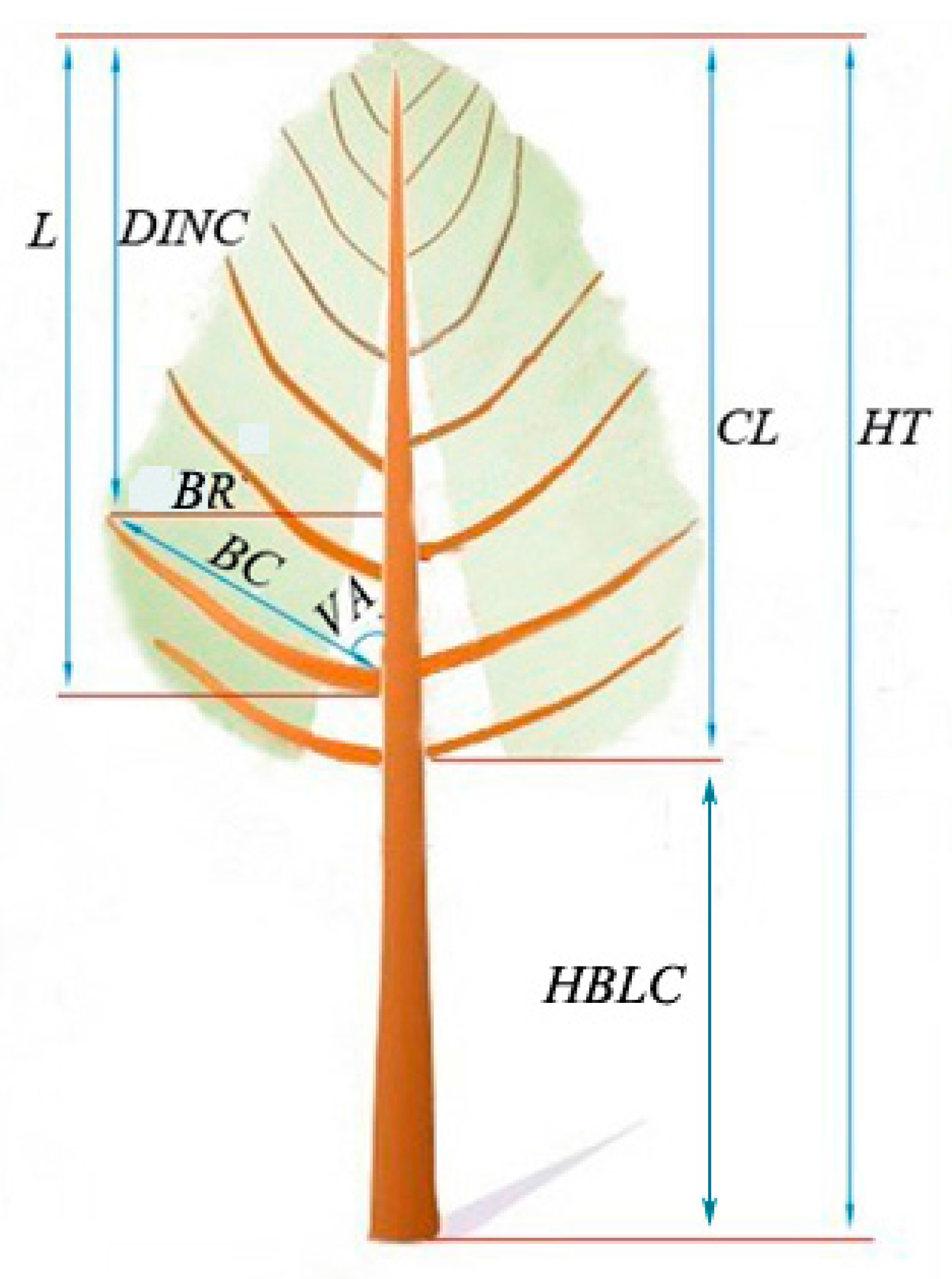
Figure 2.
Effects of stand age and stand density on the crown profile based on the dummy variable approach. (A) reflects the effect of stand age on the crown profile and (B) reflects the effect of stand density on the crown profile. Age group 1 represents the stand age lower than 20 years, Age group 2 between 21 and 30 years, Age group 3 of 31–40 years, and Age group 4 between 41 and 60 years. Density group 1 represents the stand density lower than 1000 trees ha−1; Density group 2 between 1000 and 2000 trees ha−1; Density group 3 between 2000 and 3000 trees ha−1, and Density group 4 of larger than 3000 trees ha−1.
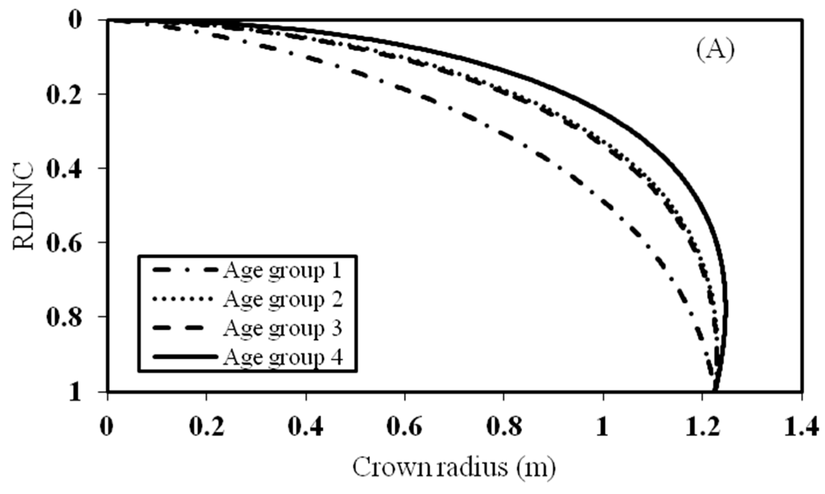

Figure 3.
Observed largest crown radius (LCR) plotted against the predicted crown radius by the quantile regression (A) and quantile regression for linear mixed-effects model (B).
Figure 3.
Observed largest crown radius (LCR) plotted against the predicted crown radius by the quantile regression (A) and quantile regression for linear mixed-effects model (B).

Figure 4.
The fitted outer crown profiles against the observed crown radius for three sample trees from three same plots (stand age is 20 years and stand density is 3950 trees ha−1 for tree (A1–A3); stand age is 33 years and stand density is 1883 trees ha−1 for trees (B1–B3); stand age is 44 years and stand density is 1640 trees ha−1 for trees (C1–C3)) for the planted Pinus sylvestris var. mongolica trees.
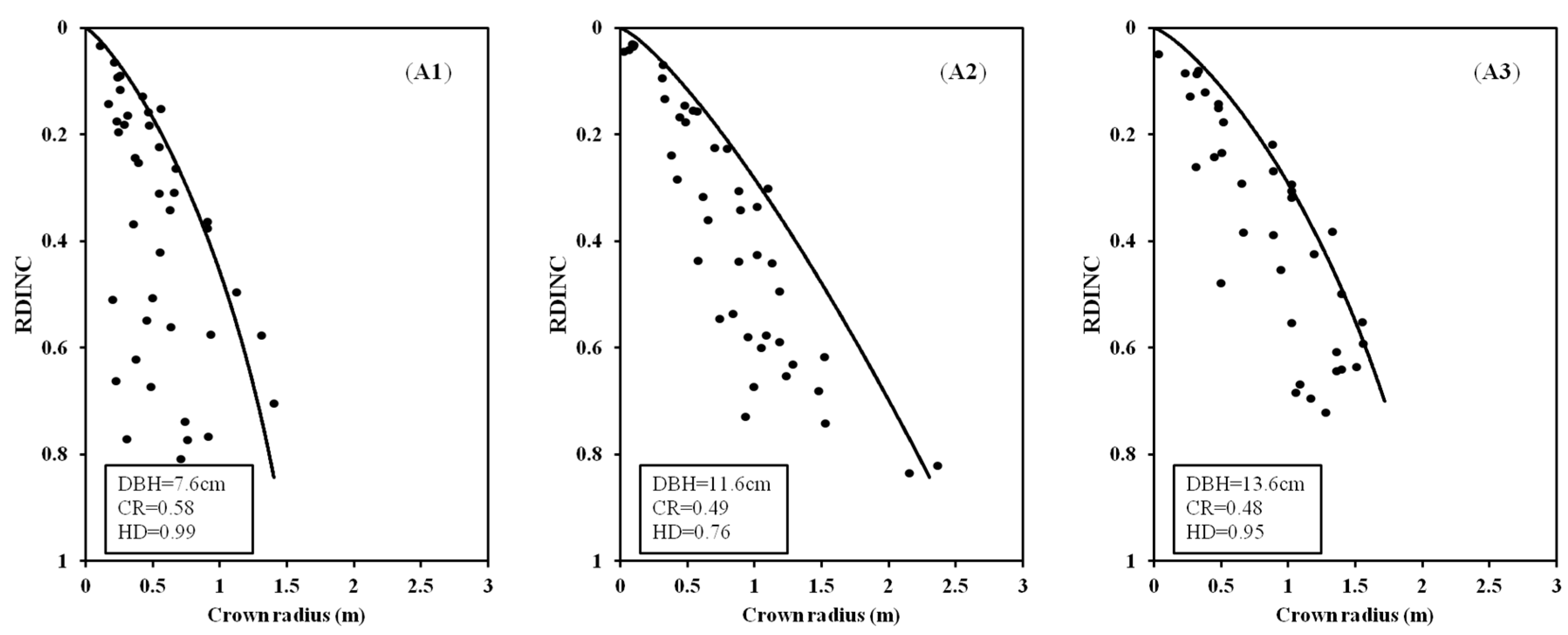
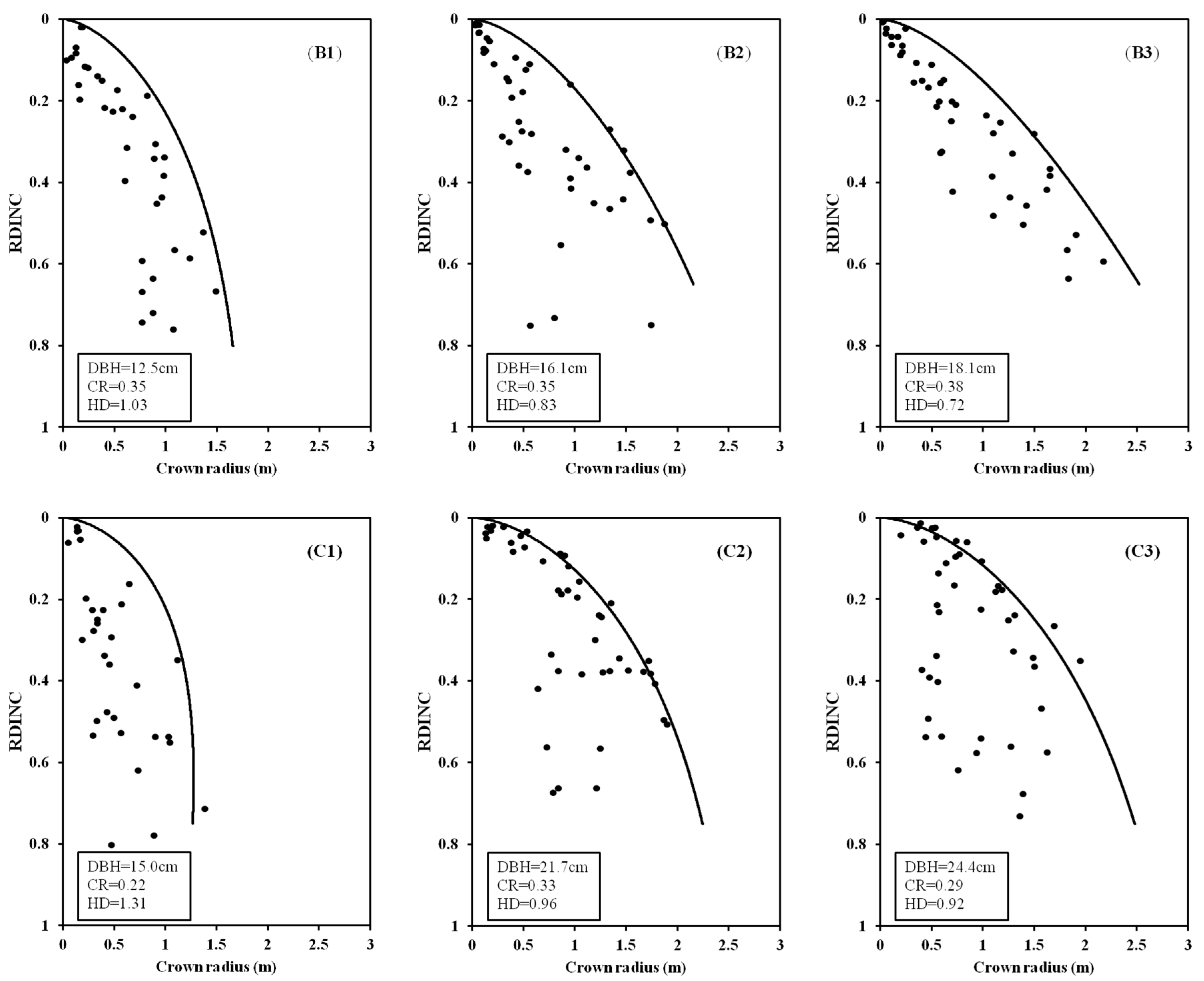
Figure 5.
Effect of stand age, stand density and ratio of tree height to diameter at the breast height (HD) on the crown profile keeping other variables as constant.
Figure 5.
Effect of stand age, stand density and ratio of tree height to diameter at the breast height (HD) on the crown profile keeping other variables as constant.


Table 1.
Summary of the stand attributes for the 15 sample plots.
| Plot Number | Stand Age (Year) | Stand Density (Trees ha−1) | Mean DBH (cm) | Mean Tree Height (m) | Stand Volume (m3 ha−1) | Stand Basal Area (m2 ha−1) | Numbers of Sample Trees |
|---|---|---|---|---|---|---|---|
| 1 | 42 | 385 | 29.1 | 18.2 | 221.9 | 25.81 | 5 |
| 2 | 42 | 650 | 23.6 | 16.9 | 227.2 | 28.86 | 5 |
| 3 | 26 | 783 | 15.2 | 8.6 | 100.1 | 14.99 | 5 |
| 4 | 33 | 1883 | 13.3 | 13.9 | 168.8 | 27.11 | 5 |
| 5 | 18 | 3633 | 8.6 | 5.7 | 117.0 | 22.37 | 5 |
| 6 | 38 | 1025 | 19.1 | 15.4 | 220.4 | 30.33 | 5 |
| 7 | 44 | 1640 | 19.0 | 21.1 | 347.7 | 47.98 | 5 |
| 8 | 33 | 3840 | 10.6 | 9.9 | 163.9 | 28.62 | 5 |
| 9 | 43 | 1100 | 20.1 | 16.5 | 264.3 | 35.73 | 5 |
| 10 | 31 | 2025 | 13.4 | 11.7 | 192.5 | 30.33 | 5 |
| 11 | 46 | 450 | 29.6 | 20.7 | 287.0 | 32.86 | 5 |
| 12 | 38 | 1220 | 19.2 | 16.0 | 267.9 | 36.65 | 5 |
| 13 | 45 | 1217 | 21.0 | 19.5 | 344.0 | 44.36 | 5 |
| 14 | 20 | 3950 | 9.7 | 7.7 | 77.7 | 31.01 | 5 |
| 15 | 12 | 2350 | 7.1 | 4.3 | 36.2 | 9.62 | 6 |
Table 2.
Descriptive statistics of sample trees and all branches for 76 planted Pinus sylvestris var. mongolica trees.
Table 2.
Descriptive statistics of sample trees and all branches for 76 planted Pinus sylvestris var. mongolica trees.
| Statistics | Tree Variables (N = 76) | Branch Variables (N = 3658) | |||||
|---|---|---|---|---|---|---|---|
| DBH (cm) | HT (m) | CL | BL (cm) | BC (cm) | VA (°) | BD (mm) | |
| Mean | 17.9 | 14.3 | 5.4 | 130 | 121 | 47 | 2.02 |
| Std | 7.2 | 5.2 | 1.6 | 88 | 82 | 16 | 1.10 |
| Min | 6.0 | 3.5 | 2.6 | 3 | 3 | 10 | 0.09 |
| Max | 34.5 | 22.5 | 10.9 | 536 | 521 | 150 | 7.16 |
Note: DBH is the diameter at breast height; HT is the total tree height; CL is the crown length; BL is the branch length; BC is the branch chord length; VA is the branch angle; and BD is the branch diameter.
Table 3.
Mean error and mean absolute error produced by power-exponential equation, modified Kozak equation and simple polynomial equation.
Table 3.
Mean error and mean absolute error produced by power-exponential equation, modified Kozak equation and simple polynomial equation.
| Crown | Models | Power-Exponential Equation | Modified Kozak Equation | Simple Polynomial Equation |
|---|---|---|---|---|
| Total tree | Ra2 | 0.79 | 0.77 | 0.76 |
| RMSE | 0.3544 | 0.3675 | 0.3722 | |
| AIC | 762 | 835 | 858 | |
| Mean error | 0.0065 | 0.0065 | 0.0079 | |
| Mean absolute error | 0.2579 | 0.2664 | 0.2717 | |
| Light crown | Mean error | 0.0224 | 0.0209 | 0.0206 |
| Mean absolute error | 0.2467 | 0.2511 | 0.2588 | |
| Shade crown | Mean error | −0.1155 | −0.1039 | −0.1357 |
| Mean absolute error | 0.3436 | 0.3835 | 0.3713 bottom boder |
Table 4.
Estimates for the parameters of the dummy variable regression model for the stand age and stand density (Equations (10) and (11)).
Table 4.
Estimates for the parameters of the dummy variable regression model for the stand age and stand density (Equations (10) and (11)).
| Dummy Variables | Parameters | a1 | a2 | a30 | a31 | a32 | a33 | a4 | a5 |
|---|---|---|---|---|---|---|---|---|---|
| Stand age | Estimates | 0.3283 | 0.8064 | −0.1450 | −0.4671 | −0.4477 | −0.6057 | 0.4686 | −1.3186 |
| Std | 0.0296 | 0.0768 | 0.1175 | 0.1605 | 0.2065 | 0.1803 | 0.2818 | 0.2936 | |
| Stand density | Estimates | 0.3385 | 0.7571 | −0.4034 | −0.3886 | −0.1364 | 0.1067 | 0.4734 | −1.3342 |
| Std | 0.0296 | 0.0752 | 0.1539 | 0.2087 | 0.1148 | 0.1747 | 0.2752 | 0.2841 |
Table 5.
The statistics for the third marginal model, quantile regression model (with the 0.90th, 0.95th, and 0.99th quantile), and the quantile regression for linear mixed-effects model for the 0.95th quantile.
Table 5.
The statistics for the third marginal model, quantile regression model (with the 0.90th, 0.95th, and 0.99th quantile), and the quantile regression for linear mixed-effects model for the 0.95th quantile.
| Models | R2 | Var(εp) | [E(εp)]2 | MEP | MAEP |
|---|---|---|---|---|---|
| M3 | 0.9380 | 0.2291 | 0.0017 | 0.0388 | 0.1626 |
| q = 0.90 | 0.8789 | 0.2351 | 0.0510 | 0.2280 | 0.2312 |
| q = 0.95 | 0.9342 | 0.2312 | 0.0046 | 0.0668 | 0.1635 |
| q = 0.99 | 0.7987 | 0.3446 | 0.0577 | −0.2400 | 0.3187 |
| q = 0.95 (qrLMM) | 0.9431 | 0.2190 | 0.0026 | −0.0545 | 0.1458 |
Table 6.
Fitting statistics for the quantile regression for linear mixed-effects models of the 0.95th quantile with different random effects parameters.
Table 6.
Fitting statistics for the quantile regression for linear mixed-effects models of the 0.95th quantile with different random effects parameters.
| Random Effect | AIC | BIC | HQ | logLike |
|---|---|---|---|---|
| b1 | 1091 | 1130 | 1106 | −537 |
| b2 | 1399 | 1438 | 1414 | −691 |
| b1, b31 | 1064 | 1109 | 1081 | −523 |
| b1, b31, b4 | 1036 | 1104 | 1062 | −504 |
Table 7.
Estimates for the parameters and variance-covariance structure for the quantile regression for linear mixed-effects outer crown profile model.
Table 7.
Estimates for the parameters and variance-covariance structure for the quantile regression for linear mixed-effects outer crown profile model.
| Parameter | b1 | b2 | b31 | b32 | b33 | b4 | b5 |
|---|---|---|---|---|---|---|---|
| Estimates | 0.4084 | 0.6081 | 0.1240 | −0.0079 | 0.0001 | 1.2039 | −1.6362 |
| Std | 0.0126 | 0.0358 | 0.0783 | 0.0029 | 0.0000 | 0.1353 | 0.1461 |
Note: var(b1) = 0.0648, var(b31) = 0.8988, var(b4) = 0.0321, var(b1, b31) = 0.1875, var(b1, b4) = −0.2731, var(b31, b4) = −0.8317.
© 2017 by the authors. Licensee MDPI, Basel, Switzerland. This article is an open access article distributed under the terms and conditions of the Creative Commons Attribution (CC BY) license (http://creativecommons.org/licenses/by/4.0/).
Share and Cite
MDPI and ACS Style
Sun, Y.; Gao, H.; Li, F. Using Linear Mixed-Effects Models with Quantile Regression to Simulate the Crown Profile of Planted Pinus sylvestris var. Mongolica Trees. Forests 2017, 8, 446. https://doi.org/10.3390/f8110446
AMA Style
Sun Y, Gao H, Li F. Using Linear Mixed-Effects Models with Quantile Regression to Simulate the Crown Profile of Planted Pinus sylvestris var. Mongolica Trees. Forests. 2017; 8(11):446. https://doi.org/10.3390/f8110446
Chicago/Turabian StyleSun, Yunxia, Huilin Gao, and Fengri Li. 2017. "Using Linear Mixed-Effects Models with Quantile Regression to Simulate the Crown Profile of Planted Pinus sylvestris var. Mongolica Trees" Forests 8, no. 11: 446. https://doi.org/10.3390/f8110446
Note that from the first issue of 2016, this journal uses article numbers instead of page numbers. See further details here.