A Dynamic System of Growth and Yield Equations for Pinus patula

 ,
, 
 , ,
, , 
Abstract
:1. Introduction
2. Materials and Methods
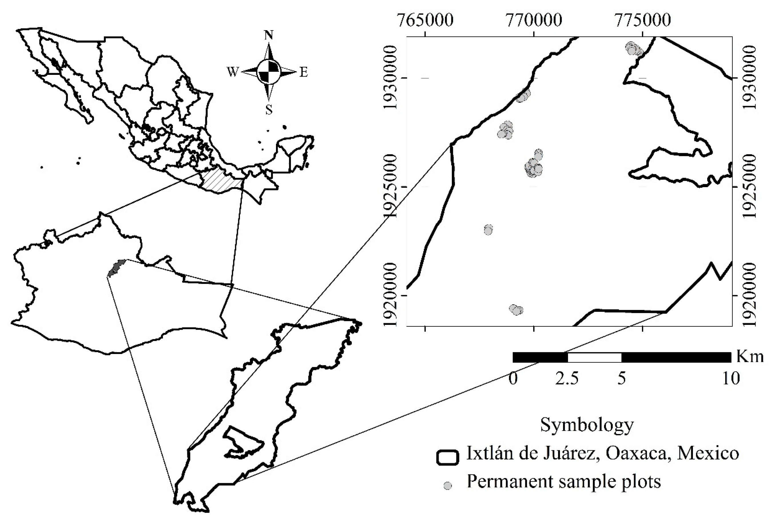
2.1. Study Area
2.2. Forest Inventory Data
2.3. Development of Compatible Models
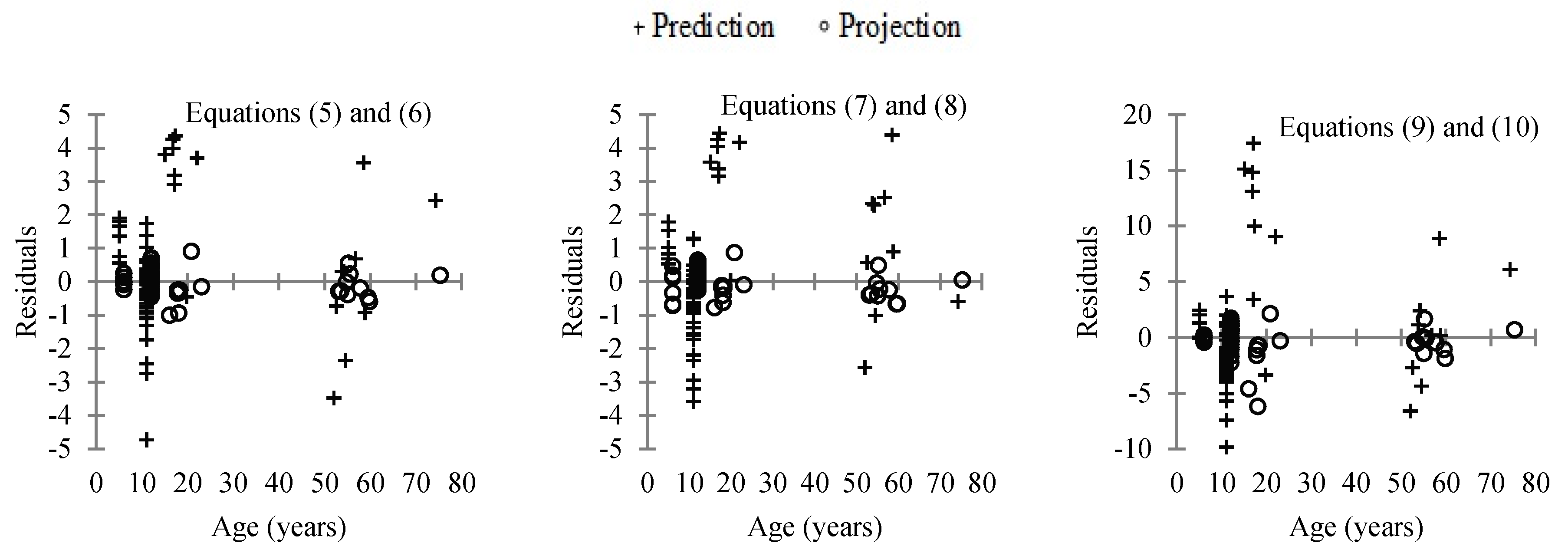
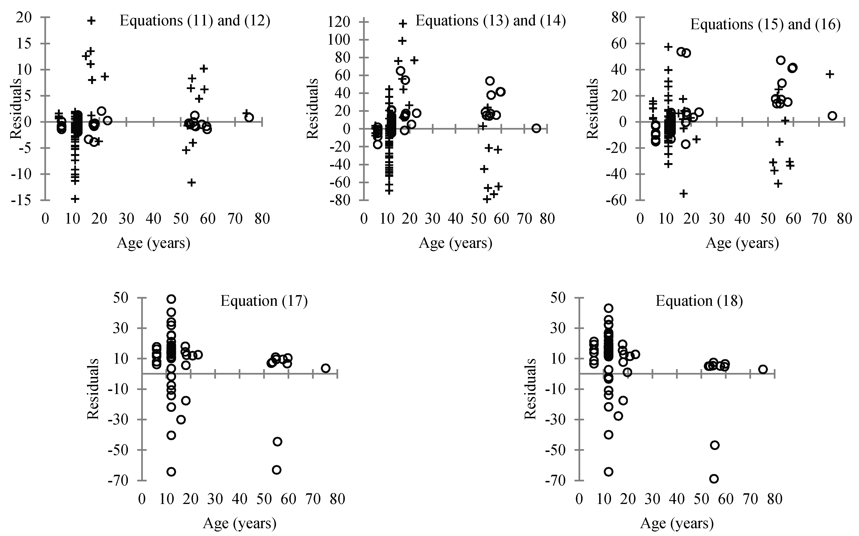
2.4. Fitting Models and Statistical Analysis
3. Results
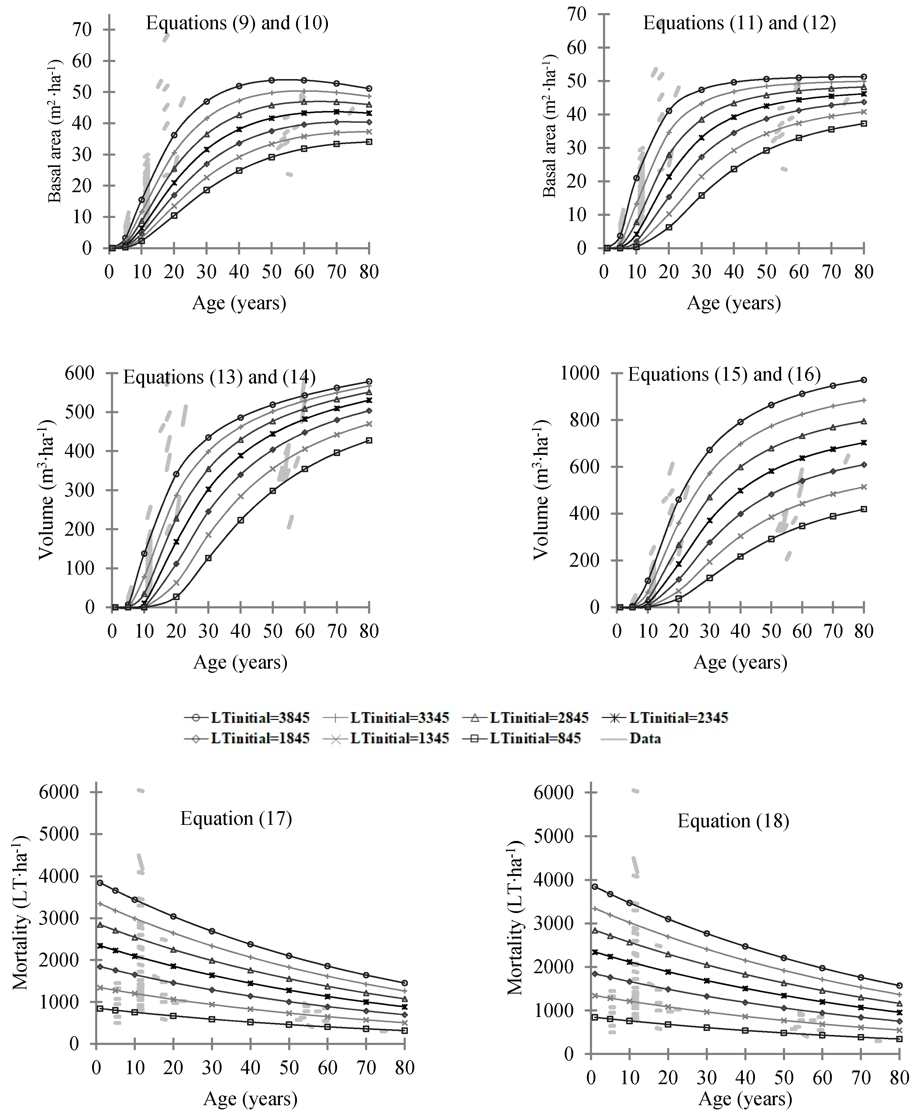
3.1. Growth Models
3.2. Using the Compatible System
4. Discussion
5. Conclusions
Supplementary Materials
Acknowledgments
Author Contributions
Conflicts of Interest
References
- Velázquez, A.; Ángeles, G.; Llanderal, T.; Román, A.; Reyes, V. Monografía de Pinus patula; Conafor-Semarnat-Colpos: Mexico City, Mexico, 2004. [Google Scholar]
- Castellanos-Bolaños, J.F.; Treviño-Garza, E.J.; Aguirre-Calderón, Ó.A.; Jiménez-Pérez, J.; Musalem-Santiago, M.; López-Aguillón, R. Estructura de bosque de pino patula bajo manejo en Ixtlán de Juárez, Oaxaca, Mexico. Madera y Bosques 2008, 14, 51–63. [Google Scholar]
- Madrigal, H.S.; Moreno, C.J.; Vázquez, C.I. Comparación de dos métodos de construcción de curvas de índice de sitio para Pinus pseudostrobus Lindl. Región Hidalgo-Zinapécuaro, Michoacán. Cienc. Nicolaita 2005, 40, 157–172. [Google Scholar]
- Vanclay, J.K. Modelling Forest Growth and Yield, Applications to Mixed Tropical Forests; CAB International: Wallingford, UK, 1994. [Google Scholar]
- Santiago-García, W.; De los Santos-Posadas, H.M.; Ángeles-Pérez, G.; Valdez-Lazalde, J.R.; Corral-Rivas, J.J.; Rodríguez-Ortiz, G.; Santiago-García, E. Modelos de crecimiento y rendimiento de totalidad del rodal para Pinus patula. Madera y Bosques 2015, 21, 95–110. [Google Scholar]
- Clutter, J.L.; Forston, J.C.; Pienaar, L.V.; Brister, G.H.; Bailey, R.L. Timber Management: A Quantitative Approach; John Wiley & Sons, Inc: New York, NY, USA, 1983. [Google Scholar]
- Bailey, R.L.; Clutter, J.L. Base-age invariant polymorphic site curves. For. Sci. 1974, 20, 155–159. [Google Scholar]
- Cieszewski, C.J.; Bailey, R.L. Generalized algebraic difference approach: Theory based derivation of dynamic site equations with polymorphism and variable asymptotes. For. Sci. 2000, 461, 116–126. [Google Scholar]
- Torres, J.M.; Magaña, O.S. Evaluación de Plantaciones Forestales; Limusa: Mexico, Mexico, 2001. [Google Scholar]
- De la Fuente, A.; Velázquez, A.; Torres, J.M.; Ramírez, H.; Rodríguez, C.; Trinidad, A. Predicción del crecimiento y rendimiento de Pinus rudis Endl., en Pueblos Mancomunados, Ixtlán, Oaxaca. Rev. Cien. For. Méx. 1998, 23, 3–8. [Google Scholar]
- Montero, M.; Fierros, A.M. Predicción del crecimiento de Pinus caribaea var. hondurensis Barr y Golf. en “La Sabana”, Oaxaca, Mexico. Rev. For. Centroam. 2000, 32, 20–25. [Google Scholar]
- Zepeda, E.M.; Acosta, M. Incremento y rendimiento maderable de Pinus montezumae Lamb., en San Juan Tetla, Puebla. Madera y Bosques 2000, 6, 15–27. [Google Scholar] [CrossRef]
- Galán, R.; De los Santos, H.M.; Valdez, J.I. Crecimiento y rendimiento maderable de Cedrela odorata L. y Tabebuia donnell-smithii Rose en San José Chacalapa, Pochutla, Oaxaca. Madera y Bosques 2008, 14, 65–82. [Google Scholar]
- Magaña, O.S.; Torres, J.M.; Rodríguez, C.; Aguirre, H.; Fierros, A.M. Predicción de la producción y rendimiento de Pinus rudis Endl. en Aloapan, Oaxaca. Madera y Bosques 2008, 14, 5–19. [Google Scholar]
- Romo, D.; Navarro, H.; De los Santos-Posadas, H.M.; Hernández, O.; López, J. Crecimiento maderable y biomasa aérea en plantaciones jóvenes de Pinus patula Schiede ex Schltdl. et Cham. en Zacualpan, Veracruz. Rev. Mex. Cien. For. 2014, 5, 78–91. [Google Scholar]
- Santiago-García, W.; De los Santos-Posadas, H.M.; Ángeles-Pérez, G.; Valdez-Lazalde, J.R.; Ramírez-Valverde, G. Sistema compatible de crecimiento y rendimiento para rodales coetáneos de Pinus patula. Rev. Fitotec. Mex. 2013, 36, 163–172. [Google Scholar]
- Servicios Técnicos Forestales de Ixtlán de Juárez. Programa de Manejo Forestal Para el Aprovechamiento y Conservación de Los Recursos Forestales Maderables de Ixtlán de Juárez. Ciclo de Corta 2015–2024; Servicios Técnicos Forestales de Ixtlán de Juárez: Oaxaca, Mexico, 2015; p. 111. [Google Scholar]
- Assmann, E. The Principles of Forest Yield Study; Pergamon Press: Oxford, UK, 1970. [Google Scholar]
- Alder, D. Estimación del Volumen Forestal y Predicción del Rendimiento Con Referencia Especial a Los Trópicos; Organización de las Naciones Unidas para la Agricultura y la Alimentación: Rome, Italy, 1980; p. 20. ISBN 92-5-300923-3. [Google Scholar]
- Jacinto-Salinas, A.H. Modelos Alométricos Para Estimar Altura de Árboles en Bosques de Pino-Encino de Ixtlán, Oaxaca; Forestry Engineer, Instituto Tecnológico del Valle Oaxaca: Oaxaca, Mexico, 2016. [Google Scholar]
- Rodríguez-Justino, R. Sistemas Compatibles de Cubicación de Árboles Individuales Para dos Especies de Interés Comercial en Ixtlán de Juárez, Oaxaca. Master’s Thesis, Universidad de la Sierra Juárez, Oaxaca, Mexico, 2017. [Google Scholar]
- Pérez-López, E. Sistema de Crecimiento y Rendimiento Maderable Para Rodales Coetáneos de Pinus patula Schiede ex Schlechtendal & Chamisso; Forestry Engineer, Universidad de la Sierra Juárez: Oaxaca, Mexico, 2017. [Google Scholar]
- Diéguez-Aranda, U.; Castedo, F.; Álvarez, J.G. Funciones de crecimiento en área basimétrica para masas de Pinus sylvestris L. procedentes de repoblaciones en Galicia. Invest. Agr. Sist. Recur. For. 2005, 14, 253–266. [Google Scholar]
- Pienaar, L.V.; Page, H.; Rheney, J.W. Yield prediction for mechanically site-prepared slash pine plantations. South. J. Appl. For. 1990, 14, 104–109. [Google Scholar]
- Hui, G.; Gadow, K. Zur Modellierung der Bestandesgrundflächementwicklung dargestellt am Beispiel der Baumart Cunninghamia lanceolata. Allgemeine Forst- und Jagdzeitung 1993, 164, 144–145. [Google Scholar]
- Santiago-García, W. Modelos de Crecimiento y Rendimiento Maderable Para Pinus oaxacana Mirov, de Ixtlán de Juárez, Oaxaca; Forestry Engineer, Instituto Tecnológico del Valle de Oaxaca: Oaxaca, Mexico, 2006. [Google Scholar]
- Zhao, D.; Borders, B.; Wang, M.; Kane, M. Modeling mortality of second-rotation loblolly pine plantations in the Piedmont/Upper Coastal Plain and Lower Coastal Plain of the southern United States. For. Ecol. Manage 2007, 252, 132–143. [Google Scholar] [CrossRef]
- SAS Institute Inc. SAS/ETS® 9.3 User’s Guide; SAS Institute Inc.: Cary, NC, USA, 2011. [Google Scholar]
- Borders, B.E.; Souter, R.A.; Bailey, R.L.; Ware, K.D. Percentile-based distributions characterize forest stand tables. For. Sci. 1987, 33, 570–576. [Google Scholar]
- Borders, B.E.; Patterson, W.D. Projecting stand tables: A comparison of the Weibull diameter distribution method, a percentile-based projection method, and a basal area growth projection method. For. Sci. 1990, 36, 413–424. [Google Scholar]
- Cancino, J. Dendrometría Básica; Universidad de Concepción: Concepción, Chile, 2006; p. 124. [Google Scholar]
- Gadow, K.V.; Real, P.; Álvarez, J.G. Modelización del Crecimiento y la Evolución de Los Bosques; IUFRO World Series: Viena, Austria, 2001. [Google Scholar]
- Martínez-Zurimendi, P.; Domínguez-Domínguez, M.; Juárez-García, A.; López-López, L.M.; De la Cruz-Arias, V.; Álvarez-Martínez, J. Índice de sitio y producción maderable en plantaciones forestales de Gmelina arborea en Tabasco, Mexico (Ensayo). Rev. Fitotec. Mex. 2015, 38, 415–425. [Google Scholar]


| Variable | Mean | Standard Deviation | Minimum | Maximum |
|---|---|---|---|---|
| A1 | 18.22 | 16.93 | 5.00 | 74.25 |
| A2 | 19.22 | 16.93 | 6.00 | 75.25 |
| DH1 | 14.78 | 6.35 | 4.55 | 34.85 |
| DH2 | 16.00 | 6.17 | 6.32 | 35.41 |
| DBH1 | 13.37 | 6.63 | 5.75 | 39.21 |
| DBH2 | 14.44 | 6.36 | 7.14 | 39.84 |
| BA1 | 21.22 | 14.06 | 1.35 | 66.53 |
| BA2 | 23.82 | 13.46 | 2.59 | 68.26 |
| V1 | 160.76 | 159.59 | 3.62 | 618.24 |
| V2 | 191.56 | 169.73 | 9.01 | 665.33 |
| LT1 | 1525.38 | 1024.50 | 300.00 | 6050.00 |
| LT2 | 1510.61 | 1006.83 | 300.00 | 6025.00 |
| Indicator | Equations |
|---|---|
| Sum of squares of error (SSE) | |
| Root of mean square error (RMSE) | |
| Coefficient of determination adjusted by the number of parameters (R2adj) | |
| Absolute average bias () | |
| Akaike information criterion (AIC) |
| Equation | SSE | RMSE | R2-adj | AIC | |
|---|---|---|---|---|---|
| Prediction | |||||
| 5 (DBH1) | 316.4 | 2.232 | 0.886 | 0.097 | 111.45 |
| 7 (DBH1) | 337.5 | 2.306 | 0.879 | 0.020 | 115.71 |
| 9 (BA1) | 2102.2 | 5.754 | 0.831 | 0.344 | 236.43 |
| 11 (BA1) | 2393.2 | 6.139 | 0.808 | 0.350 | 244.99 |
| 13 (V1) | 121,918.0 | 43.646 | 0.925 | 6.825 | 502.42 |
| 15 (V1) | 24,648.7 | 19.625 | 0.985 | 1.779 | 396.91 |
| Projection | |||||
| 6 (DBH2) | 9.2 | 0.378 | 0.997 | 0.028 | −121.83 |
| 8 (DBH2) | 8.6 | 0.364 | 0.997 | 0.045 | −126.81 |
| 10 (BA2) | 117.8 | 1.351 | 0.990 | 0.041 | 46.24 |
| 12 (BA2) | 70.7 | 1.047 | 0.994 | 0.207 | 12.58 |
| 14 (V2) | 20,373.3 | 17.704 | 0.989 | 9.462 | 384.33 |
| 16 (V2) | 15,255.0 | 15.320 | 0.992 | 4.145 | 365.24 |
| 17 (LT2) | 103,635.0 | 39.930 | 0.998 | 3.901 | 487.69 |
| 18 (LT2) | 104,208.0 | 40.040 | 0.998 | 3.839 | 488.06 |
| Equations | Parameter | Estimate | Standard Error | Pr > |t| | Equations | Parameter | Estimate | Standard Error | Pr > |t| |
|---|---|---|---|---|---|---|---|---|---|
| (5) and (6) | β0 | 2.478 | 0.354 | <0.0001 | (7) and (8) | β0 | −2.568 | 0.557 | <0.0001 |
| β1 | −2.729 | 0.730 | <0.0004 | β1 | 0.705 | 0.053 | <0.0001 | ||
| β2 | −0.204 | 0.033 | <0.0001 | β2 | 0.184 | 0.025 | <0.0001 | ||
| β3 | 0.656 | 0.067 | <0.0001 | β3 | 2.329 | 0.194 | <0.0001 | ||
| (9) and (10) | β0 | −3.613 | 0.599 | <0.0001 | (11) and (12) | β0 | −10.712 | 0.641 | <0.0001 |
| β1 | −6.392 | 1.468 | <0.0001 | β1 | 0.095 | 0.021 | <0.0001 | ||
| β2 | 0.566 | 0.053 | <0.0001 | β2 | 0.596 | 0.060 | <0.0001 | ||
| β3 | 1.149 | 0.120 | <0.0001 | β3 | 3.722 | 0.250 | <0.0001 | ||
| (13) and (14) | δ0 | 2.843 | 0.128 | <0.0001 | (15) and (16) | δ0 | 0.778 | 0.043 | <0.0001 |
| δ1 | −1.725 | 0.120 | <0.0001 | δ1 | −13.580 | 0.627 | <0.0001 | ||
| δ2 | 0.278 | 0.034 | <0.0001 | δ2 | 1.072 | 0.032 | <0.0001 | ||
| (17) | α1 | −0.012 | 0.003 | <0.0001 | (18) | α1 | −0.00039 | 0.000 | <0.0001 |
| A | LT | DH | DBH | BA | V | CAI | MAI |
|---|---|---|---|---|---|---|---|
| 5 | 1500 | 2.41 | 2.76 | 0.27 | 0.23 | 0.05 | 0.05 |
| 6 | 1482 | 3.40 | 3.80 | 0.75 | 1.05 | 0.82 | 0.17 |
| 7 | 1463 | 4.47 | 4.86 | 1.59 | 3.24 | 2.19 | 0.46 |
| 8 | 1446 | 5.57 | 5.91 | 2.82 | 7.64 | 4.40 | 0.96 |
| 9 | 1428 | 6.69 | 6.94 | 4.43 | 14.97 | 7.33 | 1.66 |
| 10 | 1410 | 7.81 | 7.93 | 6.36 | 25.63 | 10.66 | 2.56 |
| 11 | 1393 | 8.91 | 8.89 | 8.53 | 39.70 | 14.07 | 3.61 |
| 12 | 1376 | 10.00 | 9.81 | 10.85 | 56.97 | 17.27 | 4.75 |
| 13 | 1359 | 11.06 | 10.70 | 13.26 | 77.04 | 20.06 | 5.93 |
| 14 | 1343 | 12.09 | 11.54 | 15.69 | 99.39 | 22.35 | 7.10 |
| 15 | 1326 | 13.08 | 12.34 | 18.08 | 123.49 | 24.10 | 8.23 |
| 16 | 1310 | 14.05 | 13.11 | 20.42 | 148.82 | 25.33 | 9.30 |
| 17 | 1294 | 14.98 | 13.85 | 22.66 | 174.91 | 26.09 | 10.29 |
| 18 | 1278 | 15.87 | 14.55 | 24.79 | 201.34 | 26.43 | 11.19 |
| 19 | 1262 | 16.73 | 15.22 | 26.80 | 227.78 | 26.43 | 11.99 |
| 20 | 1247 | 17.56 | 15.87 | 28.69 | 253.93 | 26.16 | 12.70 |
| 21 | 1232 | 18.36 | 16.49 | 30.45 | 279.60 | 25.66 | 13.31 |
| 22 | 1217 | 19.13 | 17.08 | 32.10 | 304.60 | 25.01 | 13.85 |
| 23 | 1202 | 19.86 | 17.65 | 33.62 | 328.83 | 24.23 | 14.30 |
| 24 | 1187 | 20.57 | 18.19 | 35.03 | 352.19 | 23.36 | 14.67 |
| 25 | 1172 | 21.26 | 18.72 | 36.33 | 374.64 | 22.44 | 14.99 |
| 26 | 1158 | 21.92 | 19.22 | 37.54 | 396.13 | 21.50 | 15.24 |
| 27 | 1144 | 22.55 | 19.71 | 38.64 | 416.67 | 20.54 | 15.43 |
| 28 | 1130 | 23.16 | 20.18 | 39.67 | 436.25 | 19.58 | 15.58 |
| 29 | 1116 | 23.75 | 20.64 | 40.61 | 454.89 | 18.64 | 15.69 |
| 30 | 1102 | 24.31 | 21.08 | 41.47 | 472.61 | 17.72 | 15.75 |
| 31 | 1089 | 24.86 | 21.50 | 42.27 | 489.44 | 16.83 | 15.79 |
| 32 | 1076 | 25.38 | 21.92 | 43.00 | 505.42 | 15.97 | 15.79 |
| 33 | 1062 | 25.89 | 22.32 | 43.68 | 520.57 | 15.15 | 15.77 |
| 34 | 1049 | 26.38 | 22.71 | 44.30 | 534.93 | 14.36 | 15.73 |
© 2017 by the authors. Licensee MDPI, Basel, Switzerland. This article is an open access article distributed under the terms and conditions of the Creative Commons Attribution (CC BY) license (http://creativecommons.org/licenses/by/4.0/).
Share and Cite
Santiago-García, W.; Pérez-López, E.; Quiñonez-Barraza, G.; Rodríguez-Ortiz, G.; Santiago-García, E.; Ruiz-Aquino, F.; Tamarit-Urias, J.C. A Dynamic System of Growth and Yield Equations for Pinus patula. Forests 2017, 8, 465. https://doi.org/10.3390/f8120465
Santiago-García W, Pérez-López E, Quiñonez-Barraza G, Rodríguez-Ortiz G, Santiago-García E, Ruiz-Aquino F, Tamarit-Urias JC. A Dynamic System of Growth and Yield Equations for Pinus patula. Forests. 2017; 8(12):465. https://doi.org/10.3390/f8120465
Chicago/Turabian StyleSantiago-García, Wenceslao, Eloísa Pérez-López, Gerónimo Quiñonez-Barraza, Gerardo Rodríguez-Ortiz, Elías Santiago-García, Faustino Ruiz-Aquino, and Juan Carlos Tamarit-Urias. 2017. "A Dynamic System of Growth and Yield Equations for Pinus patula" Forests 8, no. 12: 465. https://doi.org/10.3390/f8120465