Modeling Fuel Treatment Leverage: Encounter Rates, Risk Reduction, and Suppression Cost Impacts


1
U.S. Forest Service, Rocky Mountain Research Station, Fort Collins, CO 80526, USA
2
U.S. Forest Service, Rocky Mountain Research Station, Missoula, MT 59801, USA
3
Bureau of Business and Economic Research, University of Montana, Missoula, MT 59812, USA
*
Author to whom correspondence should be addressed.
Forests 2017, 8(12), 469; https://doi.org/10.3390/f8120469
Submission received: 4 October 2017
/
Revised: 16 November 2017
/
Accepted: 21 November 2017
/
Published: 29 November 2017
(This article belongs to the Special Issue Decision Support Approaches in Adaptive Forest Management—Selected Papers from the IUFRO 125th Anniversary Congress)
Abstract
:The primary theme of this study is the cost-effectiveness of fuel treatments at multiple scales of investment. We focused on the nexus of fuel management and suppression response planning, designing spatial fuel treatment strategies to incorporate landscape features that provide control opportunities that are relevant to fire operations. Our analysis explored the frequency and magnitude of fire-treatment encounters, which are critical determinants of treatment efficacy. Additionally, we examined avoided area burned, avoided suppression costs, and avoided damages, and combined all three under the umbrella of leverage to explore multiple dimensions with which to characterize return on investment. We chose the Sierra National Forest, California, USA, as our study site, due to previous work providing relevant data and analytical products, and because it has the potential for large, long-duration fires and corresponding potential for high suppression expenditures. Modeling results generally confirmed that fire-treatment encounters are rare, such that median suppression cost savings are zero, but in extreme years, savings can more than offset upfront investments. Further, reductions in risk can expand areas where moderated suppression response would be appropriate, and these areas can be mapped in relation to fire control opportunities.
1. Introduction
Wildland fires, an integral component of many ecosystems, can also pose grave safety concerns, result in significant socioeconomic damages, and negatively affect provision of ecosystem services. Changes in climate resulting in warmer, drier conditions along with extended fire season lengths suggest a future of increasing fire activity [1,2,3]. The joint impacts of population growth and expanded ex-urban development will likely result in more human-caused ignitions along with more homes and communities exposed to fire [4,5,6,7,8,9]. In certain fire-prone ecosystems, these challenges are compounded by legacy effects of decades of fire exclusion rendering forest conditions more conducive to extreme fire behavior that is resistant to control and can degrade forest health [10,11,12]. Given a likely future of increasing costs and losses, the need to develop more cost-effective and sustainable approaches to managing wildland fire is apparent [13,14,15,16].
A broad spectrum of fire management interventions is available, with varying degrees of capacity needs, costs, and effectiveness. These approaches can be generally characterized as preventing human-caused ignitions [17,18], preparing for and responding to unplanned ignitions [19,20,21], and, our focus here, implementing hazardous fuel and forest restoration treatments in advance of fires [22,23]. Adopting “fire-safe” principles [24] that reduce surface fuel loads, increase height to live crown, and decrease crown density have been shown to alter fire behavior and enhance responder safety [25,26,27]. When treated areas do burn, they typically do so with lower intensity, such that burn severity is lower and there are fewer undesirable effects [28]. Here, rather than model burn severity, we adopt a more socioecological values-focused approach that links changes in fire intensity to changes in fire consequences to resources and assets like structures, timber, and habitat. Another benefit of fuel treatments is that they may reduce suppression costs by dampening fire activity and associated suppression demands [29,30,31].
However, treatment options can be severely constrained or economically unviable in some landscapes, and questions persist regarding return on investment given current scales of treatment and the relative rarity of fire [32,33,34,35,36]. Expanding the footprint of treated areas and being more strategic in the choice of where to implement treatments are two key themes for improving treatment efficacy [37,38,39]. A critical variable determining treatment efficacy is the rate at which unplanned fires encounter fuel treatments [40]. Encounter rates generally increase with increasing fire frequency, increasing area burned, and, important for our purposes here, increasing area treated. Encounter rates in turn influence treatment leverage, a metric of fuel treatment effectiveness that is often expressed as a ratio of avoided area burned to area treated [41,42].
Here, we expand the concept of leverage in two ways: (1) by exploring reductions in suppression costs in relation to fuel treatment costs, and (2) by exploring reductions in landscape-scale risk metrics in relation to risk metrics within treated areas. This expansion is premised in part on the recognition that focusing on avoided area burned may inadequately capture the effectiveness of fuel treatments, as it may not directly relate to risk reduction for highly valued resources [43]. We note that others have examined avoided area burned, avoided suppression costs, and avoided damages; here we combine all three under the umbrella of leverage to explore multiple dimensions with which to characterize return on investment.
To model fuel treatment effectiveness, we use spatial optimization to schedule fuel treatments across a landscape under different budget levels, and use fire simulation to illustrate subsequent variation in the frequency and magnitude of fire-treatment encounters and corresponding leverage metrics. The optimization model generates efficient frontiers and quantifies tradeoffs across risk reduction and thinning volume production objectives. While similar to other recent work evaluating tradeoffs across spatial treatment strategies [44,45,46], our interest here is less in evaluating these tradeoffs per se, and more in generating plausible, efficient treatment strategies for further investigation in terms of leverage.
The treatment modeling framework we present is largely patterned after the Collaborative Forest Landscape Restoration Program (CFLRP), which is designed to support large-scale implementation of socially and economically viable projects on National Forest System lands in the U.S. [47]. Our work directly targets CFLRP objectives of reducing wildfire risk and reducing wildfire management costs, and simulates landscape treatment strategies that are comparable to existing funded projects in terms of budget levels and area treated [48]. The basics of our framework align with the Risk and Cost Analysis Tools (RCAT) package [49] developed by the Forest Service, U.S. Department of Agriculture, to help project teams evaluate proposed treatment strategies. We expand upon RCAT and a CFLRP pilot study [31] by optimizing and simulating a broader range of treatment strategies, by quantifying treatment impacts in terms of integrated net value change metrics [50,51], and by using an improved econometric model of fire suppression costs [52]. Further, we design spatial treatment strategies as a function of treatment opportunities within predefined operational fire management units, with the aim of strengthening the nexus between fuel treatment and suppression response planning [53]. We present results from a case study landscape encompassing the Sierra National Forest (SNF) in California, USA, building from recent geographically relevant research on fuel treatment opportunities, fire simulation, risk assessment, and incident response planning [33,54,55,56].
2. Materials and Methods
2.1. Case Study Location
The SNF is located in east-central California, in the Forest Service’s Pacific Southwest Region. Established in 1893, the SNF spans ~525,000 hectares between ~275 and ~4250 m in elevation. The SNF has over two dozen species of trees, with California red fir (Abies magnifica), white fir (Abies concolor), ponderosa pine (Pinus ponderosa), lodgepole pine (Pinus contorta), and incense-cedar (Calocedrus decurrens) among the most commonly found in the SNF. The SNF also contains other varied flora and fauna covering rolling foothills, heavily forested elevations, and alpine landscapes [57]. In 2014 and 2015, respectively, 136,900 cubic meters and 117,640 cubic meters of timber were cut from the SNF, mostly in the form of sawtimber and to a much lesser extent, fuelwood.
In terms of historical fire regimes, over half (54%) of the SNF is a frequent fire (≤35-year fire return interval) regime of low to moderate severity (primarily in the lower elevations). Longer fire return intervals are found at higher elevations, with 31% of the SNF in a 35–200 year return interval of low-moderate severity fire. Other fire regimes include 8% barren/non-burnable, 4% replacement severity with 35–200 year return interval, 1% sparsely vegetated, 1% water, 0.2% replacement severity with a less than 35-year return interval, 0.2% longer than 200-year return interval with replacement severity, 0.0005% snow and ice, and 0.00008% indeterminate fire regime [58].
The influences of fire suppression and other factors have shifted forest composition to fire-intolerant species and resulted in substantial departure from historical fire regimes, most notably in dry, low-elevation ponderosa pine forests [59]. Over the time period from 1992–2013, the mean annual area burned by large fires (>100 ha) that ignited in the SNF was 12,472 ha, and the mean annual burn probability for the SNF was 0.0053; the median large-fire size for the fire occurrence area we modeled (see Section 2.5) was 309 ha [60]. More information on historical fire sizes and relation to contemporary burn probabilities and burn probability modeling is available in [54,55,56].
The SNF makes a useful case study location because it reflects a microcosm of many of the challenges surrounding contemporary fire and fuels management in the western U.S.: potential for large, long-duration fires; corresponding potential for high suppression expenditures; proximal at-risk human communities; accumulation of hazardous fuel loads due in part to fire exclusion; and significant treatment and restoration needs. In fact, the National Forest is home to an existing funded project under CFLRP, the Dinkey Landscape Restoration Project, a ~62,000 ha project area where the management strategy aims to “restore key features of diverse, fire-adapted forests, including heterogeneity at multiple scales, reduced surface and ladder fuels, and terrestrial and aquatic habitats for sensitive wildlife species” [59]. To provide a sense of scale, the project aims to implement mechanical treatments on approximately 14,000 ha, and prescribed fire on approximately 19,000 ha, over a 10-year planning horizon. Across the broader SNF, annual treatments rates hover around 1000–2000 ha for mechanical treatment, and 800–1200 ha for prescribed fire [61]. Here, we abstract away from the specifics of that project, and from the logistics of regulated planning processes, to explore alternative spatial treatment strategies under different budget levels across the entire SNF.
From a more practical perspective, the SNF is a well-studied location, such that many of the building blocks for our analysis are readily available. These include maps of fuel treatment constraints [33], biophysically driven fuel treatment prescriptions [54], and spatial risk assessment and response planning results [55]. Of particular note is the use of potential wildland fire operations delineations (PODs) as the spatial unit of analysis for fuel treatment prioritization. As outlined in [55], the SNF pioneered development of PODs, which are polygons whose boundary features are relevant to fire control operations (e.g., roads, ridgetops, and water bodies). PODs provide a useful spatial construct to summarize risk and plan strategic response to unplanned ignitions accordingly [62]. It has been suggested that treatment strategies could be designed to create “anchors” to facilitate fire management operations for landscapes with limited treatment opportunities [33]. Here, we build from that idea by locating and prioritizing fuel treatments within PODs, i.e., the treatment decision unit is the POD. Figure 1 presents a map of the case study landscape, with POD boundaries and suitable treatment locations identified.
2.2. Model Workflow and Leverage Metrics
Figure 2 presents the basic workflow for our treatment modeling framework. Beginning in the upper left, the existing conditions (EC) landscape is the foundation for fire behavior modeling and treatment design, and serves as the basis for creating hypothetical post-treatment (PT) landscape conditions. The primary analytical steps highlighted in this diagram are: (1) optimization to generate efficient spatial treatment strategies, and (2) stochastic fire simulation to evaluate these strategies. Additional modules not directly illustrated in this framework are treatment location, prescription, and cost modeling; spatial risk assessment; and suppression cost modeling. Optimal treatment strategies are developed as a function of treatment costs, harvest volume, feasible treatment locations, and expected net value change (eNVC; see Section 2.5). All of these measures are summarized for each POD, which as described above, is the decision unit for implementing treatments. If a POD is selected for treatment, all of the feasible treatable area within that POD is scheduled for treatment.
Boxes highlighted in grey are used in leverage calculations, the equations for which are presented in the upper right of the figure. The “optimal treatment strategies” box is highlighted in darker grey, as this is where all inputs flow and link before post-treatment conditions are simulated. Within boxes we highlight key datasets, methods, and models used, all of which are described in more detail below. All leverage metrics are calculated as ratios, with the numerator expressing the net change due to the treatment strategy, in terms of annual area burned, suppression costs, and landscape expected net value change. The denominators reflect an attribute of the treatment strategy itself, in terms of area treated, treatment cost, and expected net value change within treated areas. Individual modeling components are described below. By also calculating fire-treatment encounter rates (described below), we are able to generate frequency-magnitude distributions that characterize treatment effects on avoided annual area burned and avoided suppression costs. In other words, in addition to asking how many times simulated fires interacted with treated areas, we can also ask, for instance, how often such interactions resulted in cost savings above a certain threshold. Note that all modeling related to fuel treatments, stochastic fire simulation, and risk assessment is performed on a pixelated, or rasterized, landscape, with a pixel size of 180 × 180 m (see Section 2.5 for more detail).
2.3. Fuel Treatment Eligibility, Prescription, and Cost Modeling
We began our fuel treatment modeling by removing from consideration any locations that were not operationally or administratively feasible for mechanical treatment. To do this, we relied on previous research mapping treatment opportunities by [33], specifically using their Scenario D, which offered the loosest constraints on treatments (allows access to all timber within 610 m of existing roads on slopes <35%, and all timber within 305 m of existing roads on slopes <50%). We then used random forest modeling to assign each pixel on the landscape to a unique tree list that corresponds to an existing Forest Inventory and Analysis (FIA) plot following the methodology of [63]. FIA measures the size and species of each tree on each plot, which provides the basis for these tree lists. Predictor variables were chosen to optimize biomass predictions, and among others included a suite of vegetation variables: existing vegetation group, existing forest cover, and existing forest height. These tree list data, mapped to each pixel on the landscape, and corresponding to a unique empirical FIA plot, formed the basis for subsequent modeling of mechanical harvesting and treatment costs, as described below.
Forest treatment prescriptions simulated for the SNF are those described by [54], and are based upon existing condition canopy cover percentage within specified ranges that are then treated to a meet a canopy cover percentage specified by prescription. The treatment prescriptions also change surface fuel models, which we model as under burning performed after mechanical thinning. These treatment prescriptions were designed to reduce the rate of spread and intensity of surface fires as well as the probability of crown fire; additional details are available in [54].
To simulate these forest treatments, we used the Western Sierra variant of the Forest Vegetation Simulator (FVS) [64]. If a plot had canopy cover > 40%, a thin from below was triggered to cut trees beginning with 5 cm diameter at breast height (DBH), progressing to larger DBH’s until the treated condition canopy cover was achieved. Using FVS, we estimated cut merchantable (tree stems with 25.4 cm minimum DBH) and non-merchantable (tops and limbs of merchantable trees and whole trees less than 25.4 cm DBH) tree components. We assumed that 15% of cut stems and 15% of branchwood from cut stems would remain in the stand due to standard operating procedures in which removing all cut material is generally unachievable for ecological purposes and operational constraints. We additionally computed other plot variables required for harvest cost modeling. Examples of computed estimated plot variables include trees per hectare cut, average cubic meter per tree cut, and the residue fraction of trees cut. We also computed harvested volume for use in treatment optimization (described below).
We then estimated harvest costs for the treatments using the Fuel Reduction Cost Simulator (FRCS) [65]. We estimated treatment costs for each plot assuming mechanical ground-based whole-tree harvesting. In addition to using stand-specific information generated with the FVS, the FRCS required additional variables. We obtained mean slope and elevation from expert opinion of silvicultural specialists with the SNF [61]. Across the entire SNF, we estimated the mean percent slope at 25%, the mean elevation at 1524 m and the mean yarding distance along the mean slope at 152 m. This is admittedly a coarse approximation resulting in vegetation structure being a primary determinant of cost estimates. We did this to dramatically reduce computational time, otherwise we would have had to run thousands of unique tree list-slope-elevation combinations through FRCS. The one-way move in distance was estimated at 121 km, the average treatment area was estimated as 20 ha, and we assumed a partial cut. The average weight of cut trees was calculated as the average of species present in the treatment areas at 362 kg per cubic meter. Following this parameterization of the FRCS model, we estimated treatment costs for all plots on the landscape meeting the canopy cover ranges.
To estimate costs of under burning to dispose of activity fuels generated from implementing the crown cover reduction treatment, we employed the model developed by [66]. As with the FRCS mechanical treatment cost model, we assume a 20 ha treatment size for each entry, where treatment size is the only continuous variable. Based on the expert opinion of a fire management officer [61] of the SNF, we parameterized this cost model assuming a fuel model of logging slash, the presence of threatened and endangered species, and proximity to the wildland-urban interface. These assumptions have the effect of creating higher cost estimates (treatments are cheaper further away from human communities and from sensitive wildlife habitat). Both these and the FRCS mechanical treatment cost estimates were converted to 2012 dollars using the Gross Domestic Product deflator [67], in order to be consistent with modeled suppression costs.
The methods described above provided per-hectare treatment costs for each operationally feasible tree list present on our modeling landscape. We then further removed from consideration tree lists on the basis of low values of canopy cover reduction or trees removed per hectare to avoid estimating what would likely be artificially high treatment costs due to harvest parameters outside of what would normally be implemented on the ground. This resulted in 199 unique tree lists that collectively accounted for 49,490 ha eligible for treatment. We aggregated these results up to the POD scale according to the number of pixels assigned to each unique tree list within each POD, resulting in a total treatment cost estimate per POD.
Lastly, we applied two additional filters for treatment, requiring a minimum treatable area within a POD of 202 ha, and limiting consideration to PODs with a net negative eNVC value (meaning net loss from wildfire). Although PODs with a positive net value change (meaning net benefit) could be candidates for application of prescribed fire for resource benefit, we did not consider that option in this analysis, choosing instead to target PODs for fuel treatments where the potential to avoid loss to highly valued resources was greatest. Applying these filters resulted in 31 PODs eligible for treatment, comprising approximately 20,640 ha.
2.4. Treatment Strategy Optimization
We developed a single-period, bi-criteria integer programming formulation to maximize risk reduction (Equation (1)) and maximize volume harvested (Equation (2)). The objective to maximize risk reduction uses as a proxy the total eNVC within areas feasible for treatment within the POD. To reiterate, the decision variable is whether to treat a given POD; selecting a POD for treatment dictates that all feasible treatment locations within the POD will be treated. The only constraint is that the total amount spent on treatment at the National Forest level must be below a defined budget level (Equation (3)); here, we explored four budgetary levels: $10.5 M, $21 M, $31.5 M, and $42 M. The basic model formulation is shown below.
| index for and set of feasible PODs | |
| B | maximum allowable budget |
| summed expected net value change for POD i | |
| total board foot volume harvested for POD i | |
| total treatment cost of POD i | |
| 0/1 variable; 1 if POD i is scheduled for treatment |
Subject to:
For each of the four budget level scenarios we generated an efficient frontier comprised of twenty solutions, by iteratively fixing the level of the volume harvested objective function and maximizing the risk reduction subject to achieving that level of volume, resulting in a total of eighty optimal treatment strategies. Because of the small size of the problem, heuristics were unnecessary, and we were able to solve all iterations to optimality using the General Algebraic Modeling System (GAMS). Although this generated more solutions than we could feasibly analyze with stochastic fire simulation, evaluating the slope of these frontiers is useful information in its own right to understand how the nature of tradeoffs across objectives may vary with available budget, and we retained optimal solutions for possible exploration in future research.
We selected six treatment strategies to feed into additional simulation analysis. In each case we selected one strategy from each budget level, with two additional strategies for the $21 M budget. To do so, we first re-scaled objective function results on a (0–1) scale according to the best performing solution (i.e., highest risk reduction, highest volume production). We then applied an even weight to both objectives, added the two objective scores together, and selected the treatment solution with the highest overall score. For the $21 M case, we also selected endpoint strategies from the frontier.
2.5. Stochastic Fire Simulation, Risk Assessment, and Suppression Cost Modeling
We used the Large Fire Simulator FSim [68] to model the ignition, spread, and eventual containment of thousands of fires across the modeling landscape. Model parameterization was facilitated by leveraging previous simulations performed on the same landscape [54,55,56,69]. Daily ignition probabilities were based on logistic regression of Energy Release Component for fuel model G values (ERC-G) in a gridded dataset for the pixel in which the Trimmer Remote Automated Weather Station is located [70]. FSim generates an ensemble of artificial yearly weather sequences (comprised of ERC-G, wind speed, and wind direction), whose statistics are representative of the local weather station records [71]. Each yearly weather sequence represents a scenario under which fire ignition and behavior are simulated. For this analysis we ran FSim for 10,024 unique yearly weather scenarios. Running thousands of fire seasons is necessary to capture variation in simulated fire weather and corresponding fire activity. Past simulation performed on the same modeling landscape ran 10,000 seasons [55], which we adopted here, with minor variation due to the number of processors used. Fire growth was based on a minimum travel time algorithm [72] using the Scott and Reinhardt crown fire model [73]. Fire containment was based on daily probabilities derived from the fuel type, number of quiescent versus active growth periods, and length of quiescent versus active growth periods [74]. A pixel size of 180 × 180 m was used, created by nearest neighbor resampling of LANDFIRE c2012 landscape data [58] in native 30 m pixels; this upscaling was performed to increase computational efficiency. Fuel models were based on the 40-model set by [75]. The model was calibrated on this “existing conditions” landscape by adjusting the suppression factor (which controls the rate at which “fireline” is built to contain the fire) and the acrefract (which adjusts the number of ignitions) until the mean number and size of modeled fires closely reflected the historical observed fires in the simulation area [60]. The simulation area was larger than the SNF, in order to allow fires to ignite outside the study area and burn into it; see [54].
FSim outputs include (1) an event set of fire perimeters, (2) a raster of burn probabilities produced by tallying the number of times each pixel burned during the simulation period divided by the number of years in the simulation period, and (3) rasters of the conditional probability of six flame length categories. The same set of fire ignitions and weather was used for all landscapes (current existing conditions landscape and six post-treatment landscapes; see below). Thus, fire sizes, flame lengths, and derived fire suppression costs can be directly compared across all seven runs.
We used FSim outputs as inputs into models of fire risk and suppression cost. In the case of the former, we relied on a widely-used framework [50] that characterizes fire-related losses and benefits in terms of a weighted net value change (NVC) metric. Specifically we used FireNVC, a geospatial risk calculation tool developed by the U.S. Forest Service [51]. NVC values are derived from integrating flame length burn probabilities with resource- and asset-specific response functions that define net changes in value in terms of flame categories. These response functions are tabulations of the relative change in value if the resource or asset were to burn in one of six flame-length classes. Response function values range from −100 (greatest possible loss of resource value) to +100 (greatest increase in value), and are generated by local resource specialists (e.g., wildlife biologists). Relative importance weights can also be incorporated to differentiate resources and assets in terms of management priority, which was done in this case by forest leadership. Resources and assets in the assessment included visual resources (e.g., scenic byways), human communities, inholdings (e.g., private industrial forests), critical infrastructure (e.g., transmission lines), timber resources, watershed resources, and critical terrestrial wildlife habitat. Beneficial effects from low intensity fire were expected for timber, watershed, visual, and habitat resources; more information is available in [55].
NVC values can be calculated conditional on the occurrence of fire, or, as we use here, in terms of statistical expectations that incorporate the probability of experiencing large fire. Henceforth, we refer to the risk metric we employed as expected net value change, or eNVC. To calculate eNVC, we leveraged pre-existing data and risk assessment results from the SNF [55]. For each new hypothetical treatment landscape and accompanying FSim burn probability and flame length results, we re-ran risk calculations using techniques described in [51]. To characterize risk at the POD-level we summed all pixel-level eNVC values within each POD.
To estimate suppression costs, we leveraged a recently developed regression model of suppression costs, referred to as the Spatial Stratified Cost Index (S-SCI) [52]. This model expands upon an earlier suppression cost model (simply called SCI) used by the Forest Service [76] in a few key ways, notably by using spatial data associated with the final fire perimeter rather than the ignition point, and has been shown to have improved predictive power [52]. Whereas previous work combining stochastic fire simulation with suppression cost modeling was only able to discern possible changes in suppression costs through reductions in fire size, here factors driven by changes in both fire size and shape (e.g., proportion of different fuel types burned) can be accommodated into cost estimates. Consistent with intended use to estimate cost for nominally “large” fires, we subset the fire perimeters to include only those fires that grew to be over 100 ha, and further included only fires that ignited within the SNF. The number of fires that met these criteria varied amongst the treated runs slightly, but was near 24,000.
Inputs for the suppression cost model include: fire size; fuel dryness (i.e., maximum Energy Release Component (ERC) percentile during fire and standard deviation of ERC); proportion of fire’s area in various land ownerships (i.e., U.S. Forest Service and U.S. Department of Interior); proportion of the fire’s area in various land management designations (i.e., Wilderness, Inventoried Roadless Area, other specially designated areas); mean elevation; proportion of the fire in various slope categories; proportion of the fire in various fuel types (i.e., grass, brush, timber, and slash); housing value within the fire perimeter as well as within successive buffered distances (8 km, 16 km, 32 km) of the fire perimeter; proportion of the fire in various aspect categories; fire duration; and region. We used the same data sources as [52]: primarily the Wildland Fire Decision Support Center data downloads [77] and Landscape Fire and Resource Management Planning Tools Project fuels data for the landscape c2012 [58]. Because we were estimating costs for simulated rather than observed fires, we derived fire area from a text file output by FSim called the Fire Size List, which gives the final size of each fire ignited in FSim. In order to obtain the maximum ERC during the fire and the standard deviation during the fire, we took the fire’s duration (also obtained from the Fire Size List) and looked up the ERCs during that period in a set of binary files output by FSim that record daily ERCs. Housing value was calculated using a Python script that called the arcpy module to iteratively select for each fire all housing values inside the fire and within buffered distances of the fire and summed these housing values. For the remainder of the predictor variables, we overlaid each fire perimeter with the predictor variable raster and found the variable of interest (mean for some variables and proportion for others) using the RMRS Raster Tool’s Zonal Statistics Tool [78]. Lastly, we used a script written in R [79] to estimate per-fire costs based on these predictor variables, using the coefficients presented for the ordinary least squares model presented in [52].
The processing requirements for modeling suppression costs are noticeably higher than for risk calculations, and are similar to those of the fire simulation. Whereas risk assessment results are built from burn probabilities that are aggregated across all unique simulated seasons, suppression costs must be modeled on a fire-by-fire basis. In total, costs were calculated for nearly 150,000 large fires, across the calibration and all post-treatment runs. Only after calculating these individual fire costs could we estimate annual suppression costs, accounting for years in which no simulated fires occurred and those where several occurred. We similarly calculated distributions of annual area burned, which served as the basis for our encounter rate calculations (see below).
2.6. Fire-Treatment Encounters and Changes in Burn Probability
Similar to [40], we defined a fire-treatment encounter as the geospatial intersection of a simulated fire perimeter with at least one treated pixel. We found the number of treated pixels burned by each fire using [78], overlaying each perimeter with a raster of all treated pixels for each of the six treated landscapes. We converted the number of treated pixels burned into hectares, which enables calculation of total treated area burned per fire. We then annualized these results, calculating distributions of total treated area burned for each simulated fire season. Changes in burn probability result from fire-treatment encounters that change fire sizes due to changed rates of spread in treated areas. To calculate changes in burn probability, we used the following procedure: (1) text-based (.asc) burn probability outputs from FSim were projected and converted to ESRI geodatabase raster format; (2) the burn probability raster from each treatment scenario was subtracted from the burn probability raster from the existing conditions (untreated) scenario; (3) this difference raster was clipped to the boundary of the SNF; and (4) the mean difference was calculated.
3. Results
3.1. POD Summaries, Optimal Treatment Strategies, and Changes in Burn Probability
Once all landscape constraints were implemented, only 8.6% of the SNF was eligible for fuel treatment (Figure 1). However, this figure was several times the amount of landscape that could be treated due to budget constraints. Figure 3 presents POD-level summary statistics on total volume harvested (x-axis), total expected net value change (y-axis), and total treatment cost (bubble size), with results rescaled to a 0–1 scale. PODs colored in orange are those considered eligible for inclusion in the spatial treatment strategy, after applying filters for minimum treatable area and expected net value change. For ease of presentation, in this and subsequent figures we display negative eNVC (net loss) values on the positive y-axis, since our treatment prioritization focused only on those PODs with expected net losses. In other words, PODs with higher positive values on the y-axis represent PODs with greater loss potential. Figure 4 displays efficient frontiers for the treatment strategies across the four budget levels, along with solutions selected for simulation with FSim. The frontiers narrow and become less steep as the budget increases, suggesting that with additional resources the model does not have to face as stark tradeoffs across objectives.
The location of PODs selected for treatment in each budget scenario is presented in Figure 5. At higher budget levels, some of the treated PODs ended up being clustered together, especially in the northwestern corner of the modeling landscape, suggesting that PODs with high risk or high volume are co-located on the landscape and preferentially selected for treatment together. Future work could explore treatment strategies that exploit spatial adjacency relationships to intentionally cluster PODs.
Not surprisingly, increasing the budget increased the number of PODs treated and the total treated area (Table 1). Treated area increased in a linear fashion in response to amount invested, from approximately 4000 ha treated at $10.5 million up to approximately 16,500 ha at $42 million. The mean simulated burn probability for the calibrated (i.e., existing conditions) landscape was 0.0048, comparable to the recent historical mean of 0.0053 (see Section 2.1). Investing $10 million in fuel treatments reduced the mean burn probability of the SNF by 3.7%. Additional investments in fuel treatments reduced burn probability in a linear fashion, by approximately 3% per $10.5 million invested, with reduction in burn probability of 12% for a $42 million investment.
Figure 6 illustrates reductions in burn probability for four treatment scenarios, one at each budget level, in relation to PODs selected for treatment. Burn probabilities were reduced by the treatment within and adjacent to the treated area. Note that reduction in burn probability is negative (blue). Some pixels experienced a slight increase in burn probability (light orange), which is a phenomenon that has been seen in other modeling studies with FSim [31], and is likely attributable to either stochastic spotting within the model or treatments changing rates of spread and fire spread pathways across the landscape. Figure 7 presents a similar set of results, but focuses on reduction in burn probability in high flame length classes, where “high” flame length is defined as >1.2 m. The mean high flame length burn probability for the existing conditions, calibration SNF landscape is 0.002539. The pattern of reduction is similar to Figure 6, but the percentage reductions are higher.
Figure 8 drills down into the $10.5 M budget treatment scenario, showing the actual location of treated pixels with treated PODs, along with changes in flame length probabilities. Note the figure also expresses burn probability changes in percentage, not absolute, terms. Low flame length probabilities show reductions, but also increased within the treated area (lower middle panel), in some cases dramatically (over two orders of magnitude). In many instances these increases in low flame length probability are wholly if not more than compensated for by reductions in high flame length probability, with the net effect being a reduction in total burn probability. The probability of high flame lengths (lower right panel) experienced widespread decreases within the treated areas, adjacent to them, and even in more distant areas (e.g., the lower right corner). Figure 6, Figure 7 and Figure 8 together indicate that treatments generally reduce burn probabilities and shift pixel-specific flame length probability distributions down and to the left, such that areas are first of all less likely to burn, and second less likely to burn with high intensities that lead to negative consequences. While here we focus on resource and asset specific consequences, in general such reductions in high flame probability would likely result in overall lower expected burn severity.
3.2. Encounter Rates and Leverage Metrics
Table 2 summarizes fire-treatment encounters and treated area burned, on a per-fire basis as well as an annualized basis. Across all treatment scenarios the median values for treated area burned on both a per-fire and annualized basis are zero, which reflects the relatively low proportion of the landscape treated as well as the relatively low burn probabilities. Encounter rates are higher on an annualized basis, which captures the possibility of multiple fire-treatment interactions in a given fire season (the mean annual number of large fires is greater than 2 in all scenarios). At the highest budget level, 42% of the fire seasons have at least one fire-treatment encounter, but mean treated area burned is only 85.60 ha.
Figure 9 displays an empirical cumulative distribution function (CDF) for annual avoided area burned. Negative values correspond to increases in area burned in some seasons, a phenomenon that is also reflected in some localized increases in burn probability (Figure 6). As described above, stochastic spotting and changing preferential fire spread pathways may in some cases lead to increases in area burned, which were observed for a small fraction of seasons (0.05 to 0.10 depending on budget level). However, both the frequency and magnitude of reductions in area burned dwarfed these relatively rare and minor increases in area burned, such that mean annual reductions in area burned are positive across all budget levels (Table 3). When fire-treatment encounters do occur, the magnitude of reductions in annual area burned were roughly an order of magnitude larger than annual treated area burned (Table 2 and Table 3). For example, under the $10.5 M budget level, on average 9.12 ha of treated area burns, leading to on average a reduction of 99.27 ha in annual area burned (a factor of 11.23). These numbers in effect tell us the conditional leverage of fire-treatment encounters in terms of area burned.
Although overall reductions in mean annual area burned increased with budget, the ratio of treated area burned to reduced area burned decreased with budget. This suggests a modestly diminishing rate of return from treating more of the landscape, in terms of area burned. This result is driven in part by the objective to reduce risk, which itself is largely driven by burn probability. If leverage were determined on the basis of these fire-treatment encounters alone, the treatment strategies would come across as looking very efficient. However the treated area burned in wildfire is just a small fraction of the total area treated, and in many years, no treated area is burned.
Figure 10 displays an empirical CDF for avoided annual suppression cost. The shapes of the curves in Figure 9 and Figure 10 closely mimic each other, as changes in cost tend to track changes in size. As with avoided area burned, avoided suppression costs has a long right tail, such that in the most extreme (top 1%) of fire seasons, suppression cost savings could pay for the treatment strategies by five- to ten-fold. Table 4 presents mean annual suppression cost savings, with additional metrics related to savings in relation to treatment costs. Across treatment scenarios, cost savings of sufficient magnitude to offset treatment costs are in the 97th–98th percentile across all simulated fire seasons. The payback periods (ignoring the time value of money) are also presented, which range from 11 to 14 years. This length of time roughly aligns with the effective duration of fuel treatments in this location, suggesting that over time, suppression cost savings could at least partially recoup initial fuel treatment investments. To account for forest products revenues, in an admittedly coarse way, the table also presents the break-even revenue amounts for each strategy, using a 10 year payback period (i.e., treatment revenue +10 years of mean annual savings = treatment cost). The last row of the table presents these 10-year breakeven revenues in $ per cubic meter.
Figure 11 illustrates net changes in total POD-level eNVC, which confirm the finding that treatments reduce risk both within and often adjacent to treated PODs. Although some PODs experience minor increases in loss (negative values), likely due to increased burn probability from stochastic spotting, the number of PODs experiencing benefits, and the magnitude of those benefits, both outweigh minor increases in loss. Perhaps more telling are the total POD-level eNVC values after treatment (Figure 12). Not only are reductions in risk apparent in every treated POD, at each level of treatment, but several PODs transition from total net loss to total net benefit. The number of PODs with total net benefits increases with budget level. Here, the connection to changes in response planning becomes most evident, such that within PODs with net benefits, opportunities for moderated suppression responses may increase.
Lastly, Table 5 summarizes overall leverage metrics for avoided area burned, avoided suppression costs, and risk reduction (eNVC). As described above, the relative infrequency of fire-treatment encounters coupled with the small magnitude of impact relative to the upfront investment yields low leverage rates for area burned and suppression cost. On an annual basis, a hectare treated does not preclude a hectare from burning, and a dollar invested in treatment does not save a dollar in suppression costs, as indicated by leverage values less than 1.0. However, as stated earlier, and as demonstrated in Table 4, cost savings may accumulate over time, especially with longer effective treatment durations.
An interesting result emerges from the three solutions for the $21 M budget level. By design, solution 1 prioritized risk reduction, solution 20 prioritized volume production, and solution 10 was a midway compromise. Across those three, Solution 1 performed the best in terms of risk leverage (Table 3), as expected. However, Solution 20, which presumably prioritized economic considerations, did not have the highest cost leverage. Solution 10 in fact dominates Solution 20, performing as well or better in all three leverage categories. That Solution 10 performed the best financially is due to its relatively higher suppression cost savings, highlighting their importance in determining overall cost effectiveness.
Leverage metrics for risk reduction appear comparatively best; one unit of risk reduction within treated areas yields more than one unit of risk reduction across the landscape. This indicates that reducing burn probabilities and flame lengths both within and outside of treated areas results in reduced loss or possibly benefits highly valued resources and assets across this landscape; see [55]. This is particularly evident in Figure 7, illustrating reductions in high flame length probabilities, and in Figure 8, showing a transition to low flame length probabilities. This, for instance, reduces loss to infrastructure, which is typically modeled to experience little to no loss at low flame lengths, while wildlife habitat or fire-dependent vegetation often experiences a net benefit. More information on specifics of the risk assessment conducted on the SNF is available from the authors upon request.
4. Discussion
We developed a coupled optimization-simulation modeling framework to provide a composite picture of fuel treatment leverage in terms of avoided area burned, avoided suppression costs, and reduced risk. To parameterize and test this model, we selected a landscape encompassing the SNF, which is a relatively well-studied area, and where the authors have worked directly with local managers and staff in the past. Because of this, we were able to leverage a bevy of preexisting, vetted data and analytical products to streamline and enhance our modeling process [33,54,55,56]. Reliance on local expertise and intensive model calibration lead to what we believe are credible results in terms of simulated fire activity and corresponding leverage metrics. With that said, the treatment strategies we simulated should not be taken to be immediately implementable or to be in accord with local, collaboratively developed treatment plans, which was never our objective. Downscaled work would, for instance, need to consider what could realistically be accomplished each year given constraints on planning and capacity in addition to budget, and further would need to evaluate changes to spatial treatment strategy in light of concerns and requirements for critical terrestrial habitat. This suggests a possible avenue for future work, which will use these techniques to explore alternate strategies as well as alternative objective function formulations in a collaborative planning setting.
We explored how fire-treatment encounter rates and treated area burned varied with treated area, and in turn explored their influence on leverage metrics. We developed cumulative distribution curves for avoided area burned and avoided suppression costs, which illustrate substantial variation across simulated fire seasons. Results presented here largely corroborate findings from other related studies: opportunities for mechanical treatment can be limited because of land designation, slope, access, and other factors; fire-treatment encounters are relatively rare phenomena, but when they do occur can result in substantial changes in fire behavior both within and outside of treated areas; however, median annual reductions in area burned and suppression costs are zero [25,26,31,33,40].
The requisite of experiencing statistically rare events to offset upfront investments is another common theme in the literature, for instance, the recent finding that avoided post-fire sediment mitigation costs only offset treatment costs following extreme fire and rainstorm events [80]. Here, we found that in most years the benefits of a fuel treatment investment may be negligible from the perspective of changing fire outcomes. It is a very rare result (~1 in 10,000 years) where the investment could yield a large return in terms of avoided costs. As a changing climate possibly exacerbates fire activity, these extreme events could become more frequent, such that the return-on-investment calculus may change over time to become more attractive.
This study underscores the critical role of burn probability, which is simultaneously a key determinant of fire-treatment encounters as well as a measure of landscape-scale treatment effectiveness. Simulation modeling results demonstrated that fuel treatments can produce large reductions in burn probability and probability of high intensity fire, while increasing the probability of low intensity fire, within and near treatment boundaries. Fuel treatments reduced the overall burn probability of the SNF only modestly (3.7% reduction in burn probability with 0.7% of the National Forest treated at $10.5 million, and 12% reduction with approximately 3% treated at $42 million). While fuel treatments at this scale of investment are of little consequence to landscape-level burn probabilities, they do show promise in reducing the impact of wildfire at the site of highly valued resources and assets that could be damaged by fire. High leverage rates for eNVC suggest that these treatments can have beneficial off-site effects as well, even though reductions in burn probability were dampened outside of treated areas (Figure 6 and Figure 7). Further, the finding of positive eNVC leverage seems to confirm the notion that quantifying the avoided area burned alone may paint an incomplete picture of treatment effects relative to the exposure of and the consequences to highly valued resources and assets [43,50].
Reductions in burn probability are not universally a benefit, however, and depend on the site-specific consequences of fire. It might be desirable to increase burn probability in areas where net fire-related effects are positive, or at least to increase the conditional probability of low intensity fire for restoration objectives [81]. Here, we did demonstrate a decrease in high flame length probabilities and at least a partial transition to low flame length probabilities, in addition to broader reductions in overall burn probability. The limited opportunities for mechanical treatment suggest that application of controlled burning and managed natural fire may be necessary to change broader landscape conditions, not only on this specific landscape but across dry mixed conifer forests in the Sierra Nevada region of California [19,33,82,83].
Figure 12 may tell the most compelling story—treatment strategies can transform total POD-level risk from expected loss to expected net benefit to highly valued resources and assets. When conditions allow, managers could opportunistically use lightning-caused fires in these PODs with expected net benefits, and leverage pre-identified control features to limit fire extent within desired boundaries. That many PODs with expected net benefits are adjacent to other PODs with expected net benefits suggests that controlled burns and managed fires could expand to the scale of multiple PODs. Changes in fire management practices could, over time, provide more fire-treated areas and provide more opportunities for safe and effective fire control, as well as potential buffers to prevent growth of wildfires into PODs with expected net loss from fire.
Future improvements and refinements could unfold in a number of ways. Three extensions relate to incorporating additional treatment prescriptions as decision variables, their resultant influence of effective treatment duration, and rates of retreatment to better capture management choices and temporal dynamics [84,85]. Here, we only tangentially addressed questions of time by calculating the payback period of suppression cost savings in relation to fuel treatment costs. That leverage metrics were largely consistent across the budget levels suggests we may not have simulated treating enough of the landscape to see significant changes or economies of scale. Therefore, modeling additional treatments and retreatments over time to significantly expand the footprint of treated areas may tell a more complete picture of dynamics between treatment scale and fire-treatment interactions. Accounting for forest products revenues could offset treatment costs to fund additional treatments, which we effectively captured here by proxy through higher budget levels and sensitivity analysis of breakeven revenues, but a more robust approach could credit them to each POD within the optimization procedure directly. Adopting even longer time horizons would require modeling forest succession and accounting for the multitude of possible trajectories resulting from management and disturbance, which presents a complex computational challenge with substantial uncertainty, but can also yield important insights for policy and management [86,87].
Perhaps the most obvious and immediate extension is to more tightly couple fuel treatment and suppression response modeling [33,53]. Here, we designed treatment strategies that incorporated management units relevant to fire operations (i.e., PODs), which is but one step in enhancing the integration of fire and fuels planning. The joint design and creation of an optimal POD network through identification of potential control locations [88] and prioritizing treatments to create or enhance possible control locations [81] is an avenue ripe for future work. So too is leveraging recent advances in modeling alternative suppression response policies [56], and embedding them in a broader simulation exercise that evaluates the possibly synergistic effects of alternative fuel strategies and suppression responses. We hope that this study motivates other managers and researchers to explore opportunities to plan and implement fuel treatments that improve fire outcomes and that facilitate safe and effective suppression operations.
5. Conclusions
This study illustrates the viability and utility of integrating preventative fuel management with operational suppression response planning. The optimal fuel treatment strategies developed here have potential to reduce fire-related losses, increase fire-related benefits, and provide more options for fire managers. However, results also indicated relatively low fire-treatment encounter rates and leverage values, emphasizing the importance of strategically locating and increasing the scale of fuel treatments. Future research can build upon this work to enhance realism and provide managers with actionable information to evaluate tradeoffs and prioritize mitigation investments.
Acknowledgments
The Joint Fire Sciences Program supported this effort with grant ID 13-1-03-12; the National Fire Decision Support Center also supported this effort. Staff from the Sierra National Forest as well as the Pacific Southwest Region provided data and expertise.
Author Contributions
M.P.T. and K.L.R. conceived and designed the modeling experiments; M.P.T. and K.L.R. and J.R.H. performed the experiments; M.P.T. and K.L.R. analyzed the data; M.P.T. and K.L.R. wrote the paper.
Conflicts of Interest
The authors declare no conflict of interest. The founding sponsors had no role in the design of the study; in the collection, analyses, or interpretation of data; in the writing of the manuscript, and in the decision to publish the results.
References
- Abatzoglou, J.T.; Williams, A.P. Impact of anthropogenic climate change on wildfire across western US forests. Proc. Natl. Acad. Sci. USA 2016, 113, 11770–11775. [Google Scholar] [CrossRef] [PubMed]
- Jolly, W.M.; Cochrane, M.A.; Freeborn, P.H.; Holden, Z.A.; Brown, T.J.; Williamson, G.J.; Bowman, D.M. Climate-induced variations in global wildfire danger from 1979 to 2013. Nat. Commun. 2015, 6. [Google Scholar] [CrossRef] [PubMed]
- Riley, K.L.; Loehman, R.A. Mid-21st-century climate changes increase predicted fire occurrence and fire season length, Northern Rocky Mountains, United States. Ecosphere 2016, 7. [Google Scholar] [CrossRef]
- Syphard, A.D.; Massada, A.B.; Butsic, V.; Keeley, J.E. Land use planning and wildfire: Development policies influence future probability of housing loss. PLoS ONE 2013, 8, e71708. [Google Scholar] [CrossRef] [PubMed]
- Caggiano, M.D.; Tinkham, W.T.; Hoffman, C.; Cheng, A.S.; Hawbaker, T.J. High resolution mapping of development in the wildland-urban interface using object based image extraction. Heliyon 2016, 2, e00174. [Google Scholar] [CrossRef] [PubMed]
- Fusco, E.J.; Abatzoglou, J.T.; Balch, J.K.; Finn, J.T.; Bradley, B.A. Quantifying the human influence on fire ignition across the western USA. Ecol. Appl. 2016, 26, 2390–2401. [Google Scholar] [CrossRef] [PubMed]
- Gude, P.; Rasker, R.; Van den Noort, J. Potential for future development on fire-prone lands. J. For. 2008, 106, 198–205. [Google Scholar]
- Robinne, F.N.; Parisien, M.A.; Flannigan, M. Anthropogenic influence on wildfire activity in Alberta, Canada. Int. J. Wildland Fire 2016, 25, 1131–1143. [Google Scholar] [CrossRef]
- Theobald, D.M.; Romme, W.H. Expansion of the US wildland–urban interface. Landsc. Urban Plan. 2007, 83, 340–354. [Google Scholar] [CrossRef]
- Calkin, D.E.; Thompson, M.P.; Finney, M.A. Negative consequences of positive feedbacks in US wildfire management. For. Ecosyst. 2015, 2. [Google Scholar] [CrossRef]
- Collins, B.M.; Everett, R.G.; Stephens, S.L. Impacts of fire exclusion and recent managed fire on forest structure in old growth Sierra Nevada mixed-conifer forests. Ecosphere 2011, 2, 1–14. [Google Scholar] [CrossRef]
- Stephens, S.L.; Collins, B.M.; Biber, E.; Fulé, P.Z. US federal fire and forest policy: Emphasizing resilience in dry forests. Ecosphere 2016, 7. [Google Scholar] [CrossRef]
- Collins, R.D.; de Neufville, R.; Claro, J.; Oliveira, T.; Pacheco, A.P. Forest fire management to avoid unintended consequences: A case study of Portugal using system dynamics. J. Environ. Manag. 2013, 130, 1–9. [Google Scholar] [CrossRef] [PubMed]
- Curt, T.; Frejaville, T. Wildfire policy in Mediterranean France: How far is it efficient and sustainable? Risk Anal. 2017. [Google Scholar] [CrossRef] [PubMed]
- Olson, R.L.; Bengston, D.N.; DeVaney, L.A.; Thompson, T.A. Wildland Fire Management Futures: Insights from a Foresight Panel; Gen. Tech. Rep. NRS-152; U.S. Department of Agriculture, Forest Service, Northern Research Station: Newtown Square, PA, USA, 2015; 44p.
- Schoennagel, T.; Balch, J.K.; Brenkert-Smith, H.; Dennison, P.E.; Harvey, B.J.; Krawchuk, M.A.; Mietkiewicz, M.; Morgan, P.; Moritz, M.A.; Rasker, R.; et al. Adapt to more wildfire in western North American forests as climate changes. Proc. Natl. Acad. Sci. USA 2017, 114, 4582–4590. [Google Scholar] [CrossRef] [PubMed]
- Balch, J.K.; Bradley, B.A.; Abatzoglou, J.T.; Nagy, R.C.; Fusco, E.J.; Mahood, A.L. Human-started started wildfires expand the fire niche across the United States. Proc. Natl. Acad. Sci. USA 2017, 114, 2946–2951. [Google Scholar] [CrossRef] [PubMed]
- Prestemon, J.P.; Butry, D.T.; Thomas, D.S. The net benefits of human-ignited wildfire forecasting: The case of tribal land units in the United States. Int. J. Wildland Fire 2016, 25, 390–402. [Google Scholar] [CrossRef] [PubMed]
- North, M.P.; Stephens, S.L.; Collins, B.M.; Agee, J.K.; Aplet, G.; Franklin, J.F.; Fulé, P.Z. Reform forest fire management. Science 2015, 349, 1280–1281. [Google Scholar] [CrossRef] [PubMed]
- Haight, R.G.; Fried, J.S. Deploying wildland fire suppression resources with a scenario-based standard response model. INFOR Inf. Syst. Oper. Res. 2007, 45, 31–39. [Google Scholar] [CrossRef]
- Meyer, M.D.; Roberts, S.L.; Wills, R.; Brooks, M.; Winford, E.M. Principles of Effective USA Federal Fire Management Plans. Fire Ecol. 2015, 11. [Google Scholar] [CrossRef]
- Omi, P.N. Theory and practice of wildland fuels management. Curr. For. Rep. 2015, 1, 100–117. [Google Scholar] [CrossRef]
- Fernandes, P.M. Empirical support for the use of prescribed burning as a fuel treatment. Curr. For. Rep. 2015, 1, 118–127. [Google Scholar] [CrossRef]
- Agee, J.K.; Skinner, C.N. Basic principles of forest fuel reduction treatments. For. Ecol. Manag. 2005, 211, 83–96. [Google Scholar] [CrossRef]
- Cochrane, M.A.; Moran, C.J.; Wimberly, M.C.; Baer, A.D.; Finney, M.A.; Beckendorf, K.L.; Eidenshink, J.; Zhu, Z. Estimation of wildfire size and risk changes due to fuels treatments. Int. J. Wildland Fire 2012, 21, 357–367. [Google Scholar] [CrossRef]
- Finney, M.A.; McHugh, C.W.; Grenfell, I.C. Stand-and landscape-level effects of prescribed burning on two Arizona wildfires. Can. J. For. Res. 2005, 35, 1714–1722. [Google Scholar] [CrossRef]
- Graham, R.T.; Jain, T.B.; Loseke, M. Fuel Treatments, Fire Suppression, and Their Interaction with Wildfire and Its Impacts: The Warm Lake Experience during the Cascade Complex of Wildfires in Central Idaho, 2007; Gen. Tech. Rep. RMRS-GTR-229; U.S. Department of Agriculture, Forest Service, Rocky Mountain Research Station: Fort Collins, CO, USA, 2009; 36p.
- Moghaddas, J.J.; Craggs, L. A fuel treatment reduces fire severity and increases suppression efficiency in a mixed conifer forest. Int. J. Wildland Fire 2008, 16, 673–678. [Google Scholar] [CrossRef]
- Snider, G.; Daugherty, P.J.; Wood, D. The irrationality of continued fire suppression: An avoided cost analysis of fire hazard reduction treatments versus no treatment. J. For. 2006, 104, 431–437. [Google Scholar]
- Taylor, M.H.; Sanchez Meador, A.J.; Kim, Y.S.; Rollins, K.; Will, H. The economics of ecological restoration and hazardous fuel reduction treatments in the ponderosa pine forest ecosystem. For. Sci. 2015, 61, 988–1008. [Google Scholar] [CrossRef]
- Thompson, M.P.; Vaillant, N.M.; Haas, J.R.; Gebert, K.M.; Stockmann, K.D. Quantifying the potential impacts of fuel treatments on wildfire suppression costs. J. For. 2013, 111, 49–58. [Google Scholar] [CrossRef]
- Campbell, J.L.; Harmon, M.E.; Mitchell, S.R. Can fuel-reduction treatments really increase forest carbon storage in the western US by reducing future fire emissions? Front. Ecol. Environ. 2012, 10, 83–90. [Google Scholar] [CrossRef]
- North, M.; Brough, A.; Long, J.; Collins, B.; Bowden, P.; Yasuda, D.; Miller, J.; Sugihara, N. Constraints on mechanized treatment significantly limit mechanical fuels reduction extent in the Sierra Nevada. J. For. 2015, 113, 40–48. [Google Scholar] [CrossRef]
- Rhodes, J.J.; Baker, W.L. Fire probability, fuel treatment effectiveness and ecological tradeoffs in western US public forests. Open For. Sci. J. 2008, 1, 1–7. [Google Scholar]
- Thompson, M.; Anderson, N. Modeling fuel treatment impacts on fire suppression cost savings: A review. Calif. Agric. 2015, 69, 164–170. [Google Scholar] [CrossRef]
- Vaillant, N.M.; Reinhardt, E.D. An Evaluation of the Forest Service Hazardous Fuels Treatment Program—Are We Treating Enough to Promote Resiliency or Reduce Hazard? J. For. 2017, 115, 300–308. [Google Scholar] [CrossRef]
- Collins, B.M.; Stephens, S.L.; Moghaddas, J.J.; Battles, J. Challenges and approaches in planning fuel treatments across fire-excluded forested landscapes. J. For. 2010, 108, 24–31. [Google Scholar]
- Finney, M.A. A computational method for optimising fuel treatment locations. Int. J. Wildland Fire 2008, 16, 702–711. [Google Scholar] [CrossRef]
- Loudermilk, E.L.; Stanton, A.; Scheller, R.M.; Dilts, T.E.; Weisberg, P.J.; Skinner, C.; Yang, J. Effectiveness of fuel treatments for mitigating wildfire risk and sequestering forest carbon: A case study in the Lake Tahoe Basin. For. Ecol. Manag. 2014, 323, 114–125. [Google Scholar] [CrossRef]
- Barnett, K.; Parks, S.A.; Miller, C.; Naughton, H.T. Beyond fuel treatment effectiveness: Characterizing Interactions between fire and treatments in the US. Forests 2016, 7, 237. [Google Scholar] [CrossRef]
- Boer, M.M.; Sadler, R.J.; Wittkuhn, R.S.; McCaw, L.; Grierson, P.F. Long-term impacts of prescribed burning on regional extent and incidence of wildfires—Evidence from 50 years of active fire management in SW Australian forests. For. Ecol. Manag. 2009, 259, 132–142. [Google Scholar] [CrossRef]
- Price, O.F.; Pausas, J.G.; Govender, N.; Flannigan, M.; Fernandes, P.M.; Brooks, M.L.; Bird, R.B. Global patterns in fire leverage: The response of annual area burnt to previous fire. Int. J. Wildland Fire 2015, 24, 297–306. [Google Scholar] [CrossRef]
- Cary, G.J.; Davies, I.D.; Bradstock, R.A.; Keane, R.E.; Flannigan, M.D. Importance of fuel treatment for limiting moderate-to-high intensity fire: Findings from comparative fire modelling. Landsc. Ecol. 2017, 32, 1473–1483. [Google Scholar] [CrossRef]
- Ager, A.A.; Day, M.A.; Vogler, K. Production possibility frontiers and socioecological tradeoffs for restoration of fire adapted forests. J. Environ. Manag. 2016, 176, 157–168. [Google Scholar] [CrossRef] [PubMed]
- Stevens, J.T.; Collins, B.M.; Long, J.W.; North, M.P.; Prichard, S.J.; Tarnay, L.W.; White, A.M. Evaluating potential trade-offs among fuel treatment strategies in mixed-conifer forests of the Sierra Nevada. Ecosphere 2016, 7. [Google Scholar] [CrossRef]
- Vogler, K.C.; Ager, A.A.; Day, M.A.; Jennings, M.; Bailey, J.D. Prioritization of forest restoration projects: Tradeoffs between wildfire protection, ecological restoration and economic objectives. Forests 2015, 6, 4403–4420. [Google Scholar] [CrossRef]
- Schultz, C.A.; Jedd, T.; Beam, R.D. The Collaborative Forest Landscape Restoration Program: A history and overview of the first projects. J. For. 2012, 110, 381–391. [Google Scholar] [CrossRef]
- Collaborative Forest Landscape Restoration Program Results. Available online: https://www.fs.fed.us/restoration/CFLRP/results.shtml (accessed on 3 October 2017).
- Collaborative Forest Landscape Restoration Program Projects. Available online: https://www.fs.fed.us/restoration/CFLRP/guidance.shtml (accessed on 3 October 2017).
- Scott, J.H.; Thompson, M.P.; Calkin, D.E. A Wildfire Risk Assessment Framework for Land and Resource Management; Gen. Tech. Rep. RMRS-GTR-315; U.S. Department of Agriculture, Forest Service, Rocky Mountain Research Station: Fort Collins, CO, USA, 2013; 83p.
- Thompson, M.P.; Haas, J.R.; Gilbertson-Day, J.W.; Scott, J.H.; Langowski, P.; Bowne, E.; Calkin, D.E. Development and application of a geospatial wildfire exposure and risk calculation tool. Environ. Model. Softw. 2015, 63, 61–72. [Google Scholar] [CrossRef]
- Hand, M.S.; Thompson, M.P.; Calkin, D.E. Examining heterogeneity and wildfire management expenditures using spatially and temporally descriptive data. J. For. Econ. 2016, 22, 80–102. [Google Scholar] [CrossRef]
- Thompson, M.P. Decision making under uncertainty: Recommendations for the Wildland Fire Decision Support System (WFDSS). In Proceedings of the Large Wildland Fires Conference, Missoula, MT, USA, 19–23 May 2014; Keane, R.E., Jolly, W.M., Parsons, R., Riley, K.L., Eds.; USDA Forest Service, Rocky Mountain Research Station Proc.: Missoula, MT, USA, 2015. RMRS-P-73. [Google Scholar]
- Scott, J.H.; Thompson, M.P.; Gilbertson-Day, J.W. Examining alternative fuel management strategies and the relative contribution of National Forest System land to wildfire risk to adjacent homes—A pilot assessment on the Sierra National Forest, California, USA. For. Ecol. Manag. 2016, 362, 29–37. [Google Scholar] [CrossRef]
- Thompson, M.P.; Bowden, P.; Brough, A.; Scott, J.H.; Gilbertson-Day, J.W.; Taylor, A.; Anderson, J.; Haas, J.R. Application of Wildfire Risk Assessment Results to Wildfire Response Planning in the Southern Sierra Nevada, California, USA. Forests 2016, 7, 64. [Google Scholar] [CrossRef]
- Riley, K.L.; Thompson, M.P.; Scott, J.H.; Gilbertson-Day, J.G. A model-based framework to evaluate alternative wildfire suppression strategies. Resources 2017. in review. [Google Scholar]
- The Sierra National Forest. Available online: https://www.fs.usda.gov/sierra/ (accessed on 3 October 2017).
- Landscape Fire and Resource Management Planning Tools (LANDFIRE). Available online: https://www.landfire.gov/index.php (accessed on 3 October 2017).
- Dinkey Collaborative Landscape Restoration Strategy. Available online: https://www.fs.usda.gov/Internet/FSE_DOCUMENTS/stelprdb5351832.pdf (accessed on 3 October 2017).
- Short, K.C. A spatial database of wildfires in the United States, 1992–2011. Earth Syst. Sci. Data 2014, 6, 1–27. [Google Scholar] [CrossRef]
- Ballard, C.; Ballard, K.; Goss, J.; Rojas, R.; Tolmie, D.; Sierra National Forest Staff, CA, USA. Personal communication, 2016.
- Wei, Y.; Thompson, M.P.; Haas, J.; Dillon, G. Spatial optimization of operationally relevant large fire confine and point protection strategies: model development and test cases. Can. J. For. Res. 2017. in revisions. [Google Scholar]
- Riley, K.L.; Grenfell, I.C.; Finney, M.A. Mapping forest vegetation for the western United States using modified random forests imputation of FIA forest plots. Ecosphere 2016, 7. [Google Scholar] [CrossRef]
- Forest Vegetation Simulator. Available online: https://www.fs.fed.us/fvs/ (accessed on 3 October 2017).
- Fuel Reduction Cost Simulator. Available online: http://www.fs.fed.us/pnw/data/frcs/frcs.shtml (accessed on 3 October 2017).
- Calkin, D.; Gebert, K. Modeling fuel treatment costs on Forest Service lands in the western United States. West. J. Appl. For. 2006, 21, 217–221. [Google Scholar]
- Gross Domestic Product: Implicit Price Deflator. Available online: https://fred.stlouisfed.org/data/GDPDEF.txt (accessed on 3 October 2017).
- Finney, M.A.; McHugh, C.W.; Grenfell, I.C.; Riley, K.L.; Short, K.C. A simulation of probabilistic wildfire risk components for the continental United States. Stoch. Environ. Res. Risk Assess. 2011, 25, 973–1000. [Google Scholar] [CrossRef]
- Scott, J.H.; Thompson, M.P.; Gilbertson-Day, J.W. Exploring how alternative mapping approaches influence fireshed assessment and human community exposure to wildfire. GeoJournal 2017, 82, 201–215. [Google Scholar] [CrossRef]
- Jolly, M.; Missoula Fire Sciences Laboratory, Rocky Mountain Research Station, Missoula, MT, USA. Personal communication, 2014.
- Grenfell, I.C.; Finney, M.A.; Jolly, W.M. Simulating spatial and temporally related fire weather. In Proceedings of the VI International Conference on Forest Fire Research, Coimbra, Portugal, 15–18 November 2010; Viegas, D., Ed.; University of Coimbra: Coimbra, Portugal, 2010; p. 9. [Google Scholar]
- Finney, M.A. Fire growth using minimum travel time methods. Can. J. For. Res. 2002, 32, 1420–1424. [Google Scholar] [CrossRef]
- Scott, J.H.; Reinhardt, E.D. Assessing Crown Fire Potential by Linking Models of Surface and Crown Fire Behavior; USDA Forest Service Research Paper; U.S. Department of Agriculture, Forest Service, Rocky Mountain Research Station: Fort Collins, CO, USA, 2001.
- Finney, M.; Grenfell, I.C.; McHugh, C.W. Modeling containment of large wildfires using generalized linear mixed-model analysis. For. Sci. 2009, 55, 249–255. [Google Scholar]
- Scott, J.H.; Burgan, R.E. Standard Fire Behavior Fuel Models: A Comprehensive Set for Use with Rothermel’s Surface Fire Spread Model; General Technical Report RMRS-GTR-153; USDA Forest Service, Rocky Mountain Research Station: Fort Collins, CO, USA, 2005.
- Gebert, K.M.; Calkin, D.E.; Yoder, J. Estimating suppression expenditures for individual large wildland fires. West. J. Appl. For. 2007, 22, 188–196. [Google Scholar]
- Wildland Fire Decision Support System Data Downloads. Available online: http://wfdss.usgs.gov/wfdss/WFDSS_Data_Downloads.shtml (accessed on 3 October 2017).
- Hogland, J.; Anderson, N. Function Modeling Improves the Efficiency of Spatial Modeling Using Big Data from Remote Sensing. Big Data Cogn. Comput. 2017, 1, 3. [Google Scholar] [CrossRef]
- The R Project for Statistical Computing. Available online: https://www.r-project.org/ (accessed on 3 October 2017).
- Jones, K.W.; Cannon, J.B.; Saavedra, F.A.; Kampf, S.K.; Addington, R.N.; Cheng, A.S.; MacDonald, L.H.; Wilson, C.; Wolk, B. Return on investment from fuel treatments to reduce severe wildfire and erosion in a watershed investment program in Colorado. J. Environ. Manag. 2017, 198, 66–77. [Google Scholar] [CrossRef] [PubMed]
- Ager, A.A.; Vaillant, N.M.; McMahan, A. Restoration of fire in managed forests: A model to prioritize landscapes and analyze tradeoffs. Ecosphere 2013, 4, 1–19. [Google Scholar] [CrossRef]
- Sneeuwjagt, R.J.; Kline, T.S.; Stephens, S.L. Opportunities for improved fire use and management in California: Lessons from Western Australia. Fire Ecol. 2013, 9, 14–25. [Google Scholar]
- North, M.; Collins, B.M.; Stephens, S. Using fire to increase the scale, benefits, and future maintenance of fuels treatments. J. For. 2012, 110, 392–401. [Google Scholar] [CrossRef]
- Finney, M.A.; Seli, R.C.; McHugh, C.W.; Ager, A.A.; Bahro, B.; Agee, J.K. Simulation of long-term landscape-level fuel treatment effects on large wildfires. Int. J. Wildland Fire 2008, 16, 712–727. [Google Scholar] [CrossRef]
- Fried, J.S.; Potts, L.D.; Loreno, S.M.; Christensen, G.A.; Barbour, R.J. Inventory-based landscape-scale simulation of management effectiveness and economic feasibility with BioSum. J. For. 2016, 51, 6499–6514. [Google Scholar] [CrossRef]
- Riley, K.L.; Thompson, M.P. An uncertainty analysis of wildfire modeling. In Uncertainty in Natural Hazards: Modeling and Decision Support; Riley, K.L., Thompson, M.P., Webley, P., Eds.; Wiley and American Geophysical Union Books: New York, NY, USA, 2017; pp. 191–213. [Google Scholar]
- Barros, A.; Ager, A.; Day, M.; Preisler, H.; Spies, T.; White, E.; Pabst, R.; Olsen, K.; Platt, E.; Bailey, J.; et al. Spatiotemporal dynamics of simulated wildfire, forest management, and forest succession in central Oregon, USA. Ecol. Soc. 2017, 22. [Google Scholar] [CrossRef]
- O’Connor, C.D.; Calkin, D.E.; Thompson, M.P. An empirical machine learning method for predicting potential fire control locations for pre-fire planning and operational fire management. Int. J. Wildland Fire 2017, 26, 587–597. [Google Scholar]
Figure 1.
Sierra National Forest, POD boundaries, and feasible treatment locations. The treatment locations were determined by applying the constraint filters of [33] plus additional filters developed on the basis of economic viability (see Section 2.3). POD = potential wildland fire operations delineation, i.e., our unit of analysis for fuel treatment prioritization.
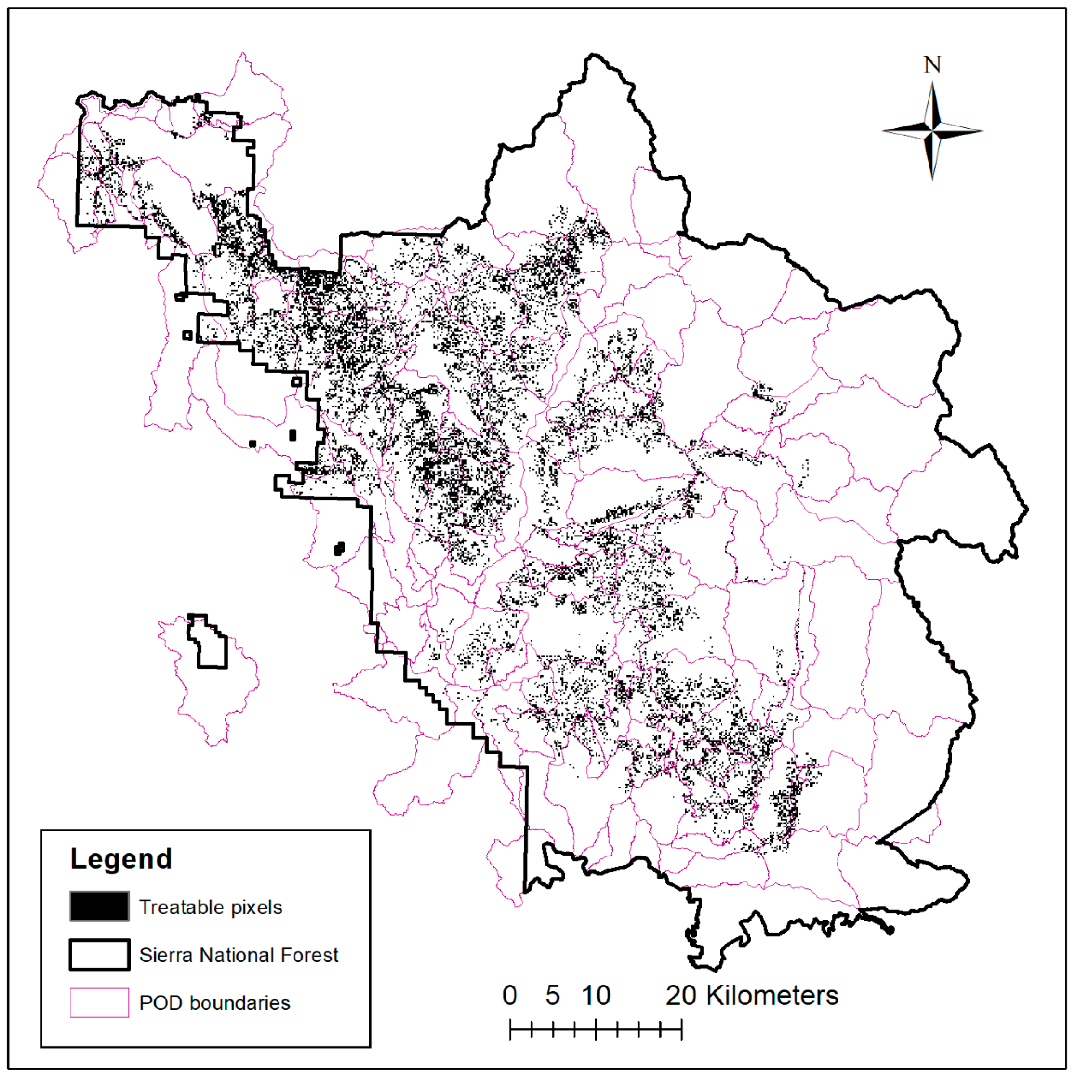
Figure 2.
Optimization-simulation modeling workflow along with leverage formulas; boxes highlighted in grey form the basis for leverage calculations. EC = existing condition; PT = post-treatment; eNVC = expected net value change; L(AB) = leverage as a function of area burned; L($) = leverage as a function of costs (U.S. dollars); L(NVC) = leverage as a function of expected net value change.
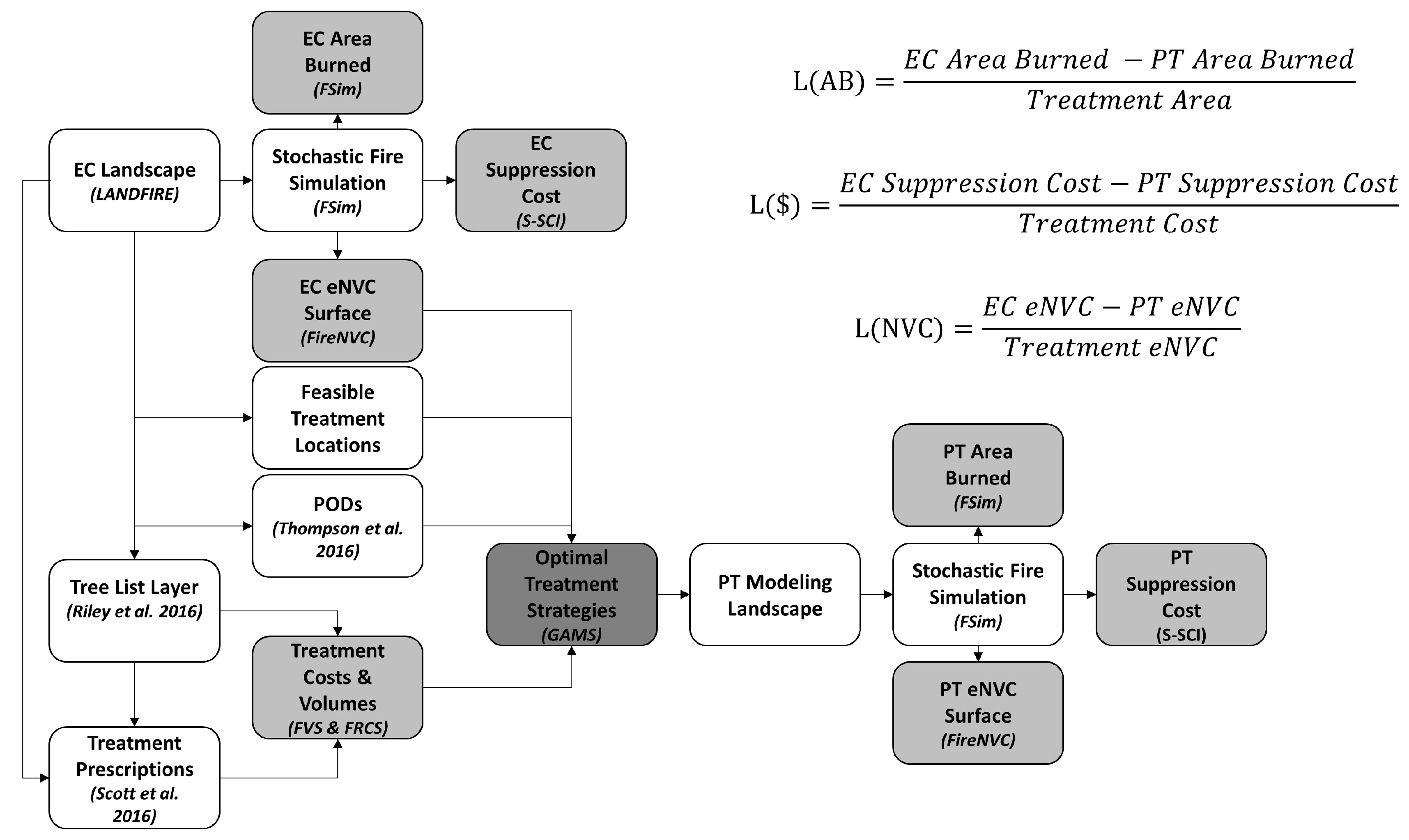
Figure 3.
POD-level summary statistics fed into the treatment optimization model; feasible PODs highlighted in orange. PODs with higher positive values on the y-axis represent PODs with greater loss potential.
Figure 3.
POD-level summary statistics fed into the treatment optimization model; feasible PODs highlighted in orange. PODs with higher positive values on the y-axis represent PODs with greater loss potential.

Figure 4.
Efficient frontiers for fuel treatment strategies, across the four budget levels, with solutions selected for simulation highlighted.
Figure 4.
Efficient frontiers for fuel treatment strategies, across the four budget levels, with solutions selected for simulation highlighted.
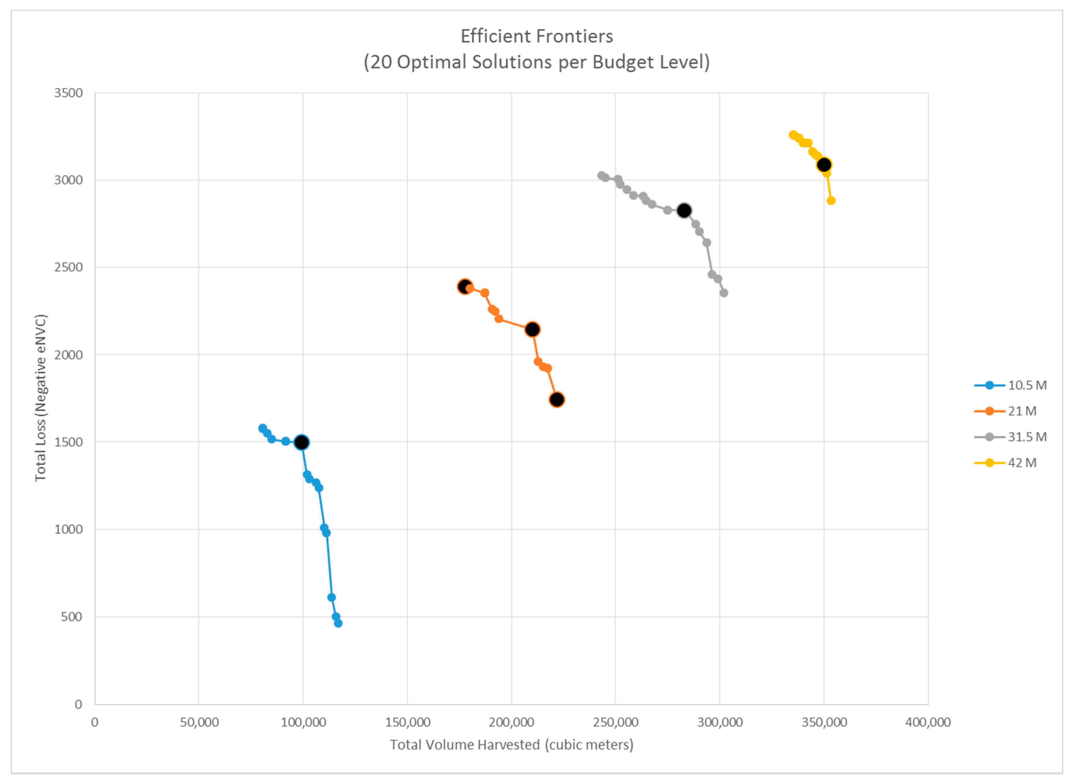
Figure 5.
Location of PODs selected for treatment in each of the six fuel treatment scenarios. The colors are unique to each POD, allowing easier viewing and identification of which PODs were selected in multiple treatment scenarios.
Figure 5.
Location of PODs selected for treatment in each of the six fuel treatment scenarios. The colors are unique to each POD, allowing easier viewing and identification of which PODs were selected in multiple treatment scenarios.
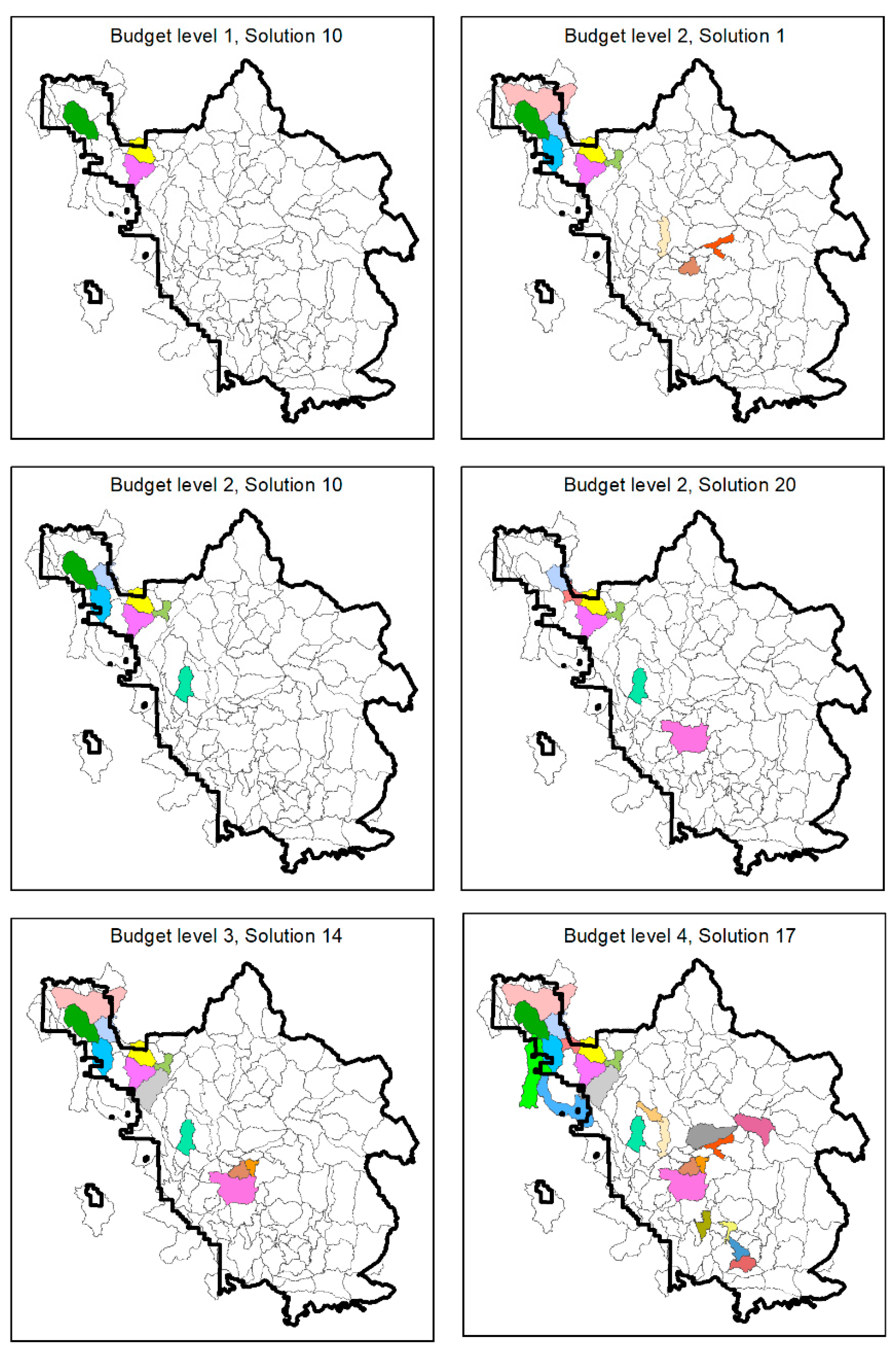
Figure 6.
Modeled fuel treatment effect on burn probabilities (BP) in the Sierra National Forest. Blue areas indicate a reduction in burn probability due to treatment, while orange areas indicate a small increase. Black outlines indicate treated PODs.
Figure 6.
Modeled fuel treatment effect on burn probabilities (BP) in the Sierra National Forest. Blue areas indicate a reduction in burn probability due to treatment, while orange areas indicate a small increase. Black outlines indicate treated PODs.

Figure 7.
Modeled fuel treatment effect on high flame length burn probabilities (FL BP) in the Sierra National Forest. Blue areas indicate a reduction in burn probability due to treatment, while orange areas indicate a small increase. Black outlines indicate treated PODs.
Figure 7.
Modeled fuel treatment effect on high flame length burn probabilities (FL BP) in the Sierra National Forest. Blue areas indicate a reduction in burn probability due to treatment, while orange areas indicate a small increase. Black outlines indicate treated PODs.
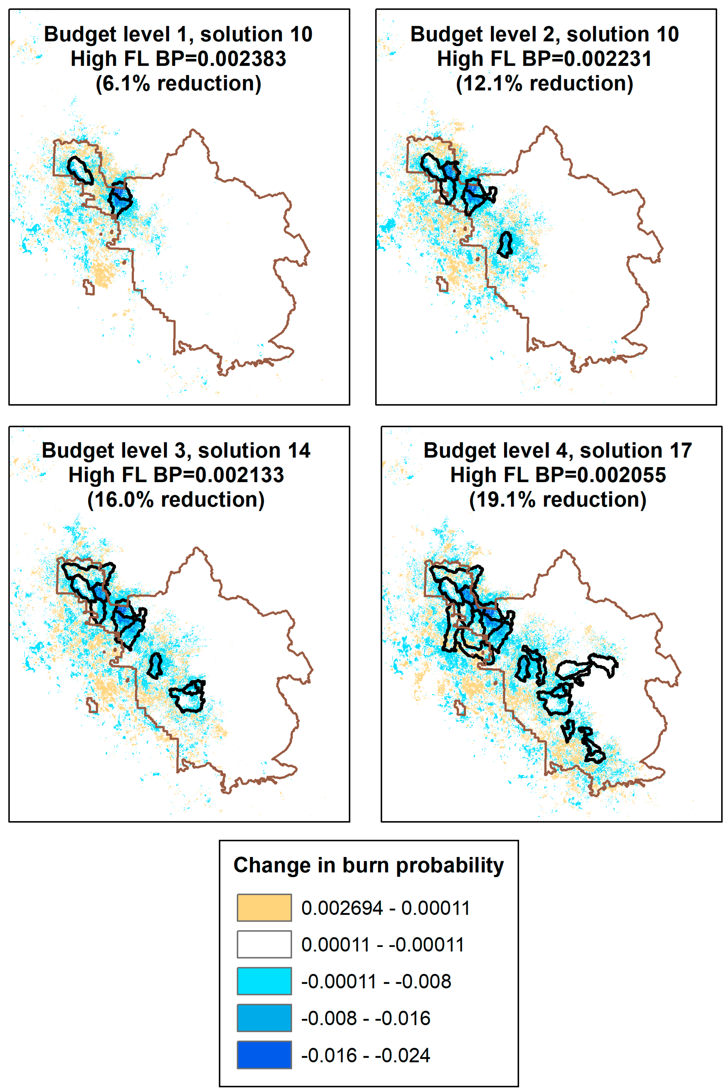
Figure 8.
Changes in burn probability (total, low flame length, and high flame length) for the $10.5 M budget treatment scenario. Each of the three windows is presented at the same scale and for the same extent. At the top left, the annual burn probability is shown for the existing conditions landscape FSim run. The top middle panel illustrates the pixels that were treated. The top right panel shows the burn probability for the post-treatment scenario. The lower left panel shows the percent reduction in burn probability (negative values indicate increases in burn probability). The two lower right panels break down reductions in burn probability according to flame length class, where “low” flame length is defined as <1.2 m. Black outlines indicate POD boundaries.

Figure 9.
Empirical cumulative distribution function (CDF) for avoided annual area burned.

Figure 10.
Empirical cumulative distribution function for avoided annual suppression cost.

Figure 11.
Net change in total POD-level eNVC under four treatment scenarios. Positive values indicate reductions in net loss. Black outlines indicate treated PODs.
Figure 11.
Net change in total POD-level eNVC under four treatment scenarios. Positive values indicate reductions in net loss. Black outlines indicate treated PODs.

Figure 12.
Total POD-level eNVC under the existing conditions (calibration) landscape, as well as four treatment scenarios. Black outlines indicate treated PODs.
Figure 12.
Total POD-level eNVC under the existing conditions (calibration) landscape, as well as four treatment scenarios. Black outlines indicate treated PODs.
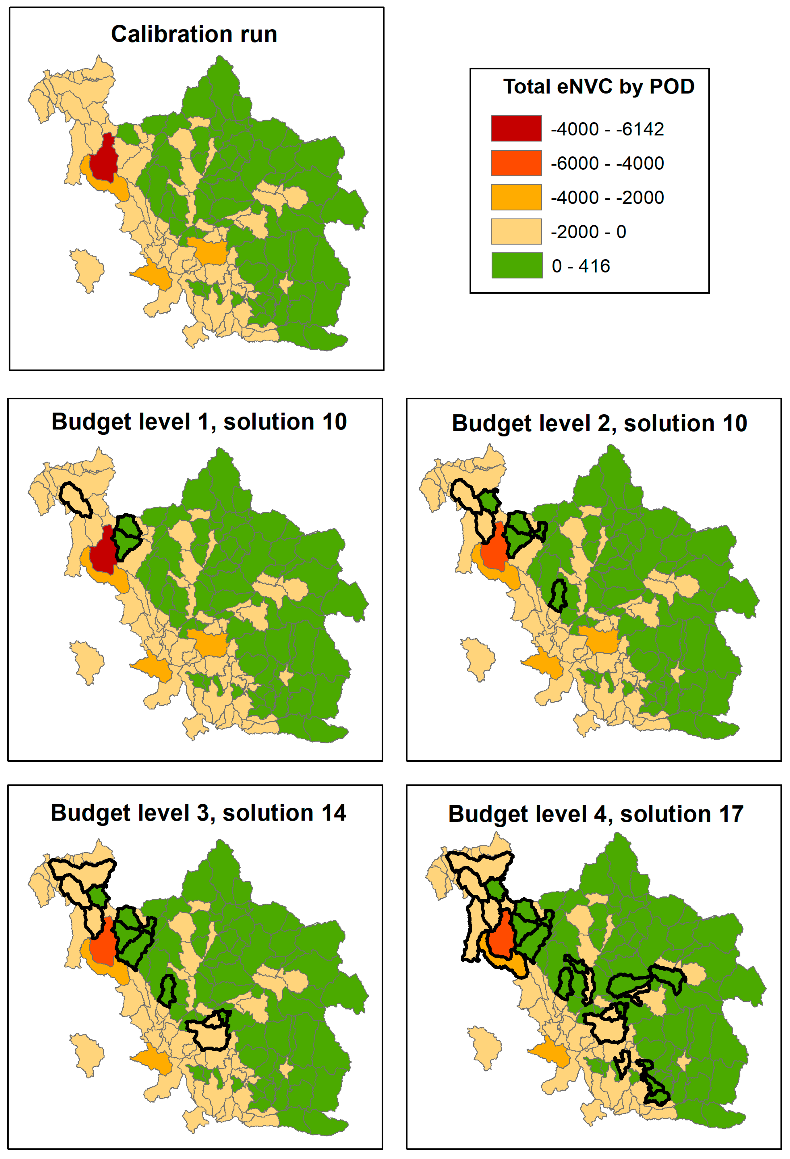

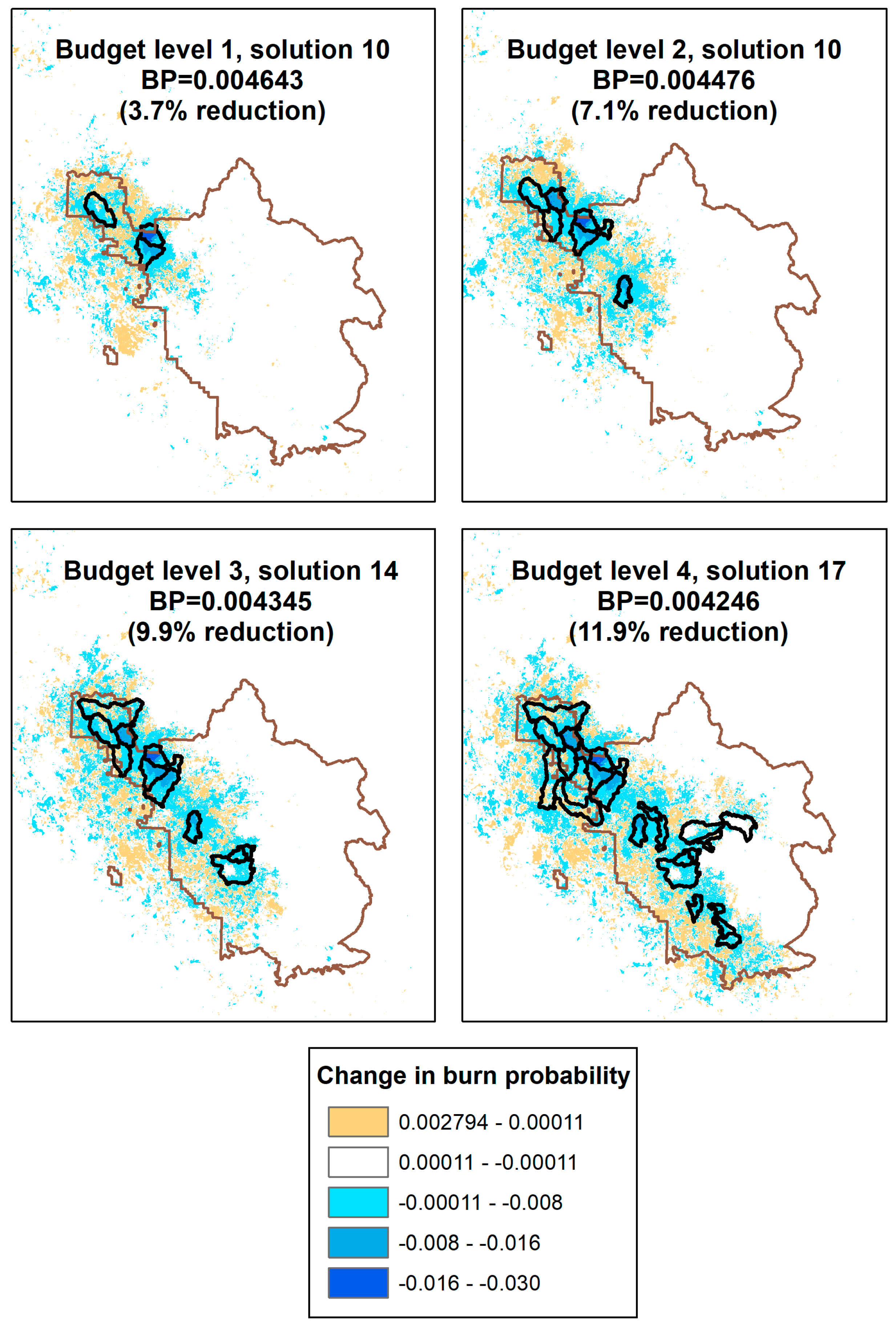
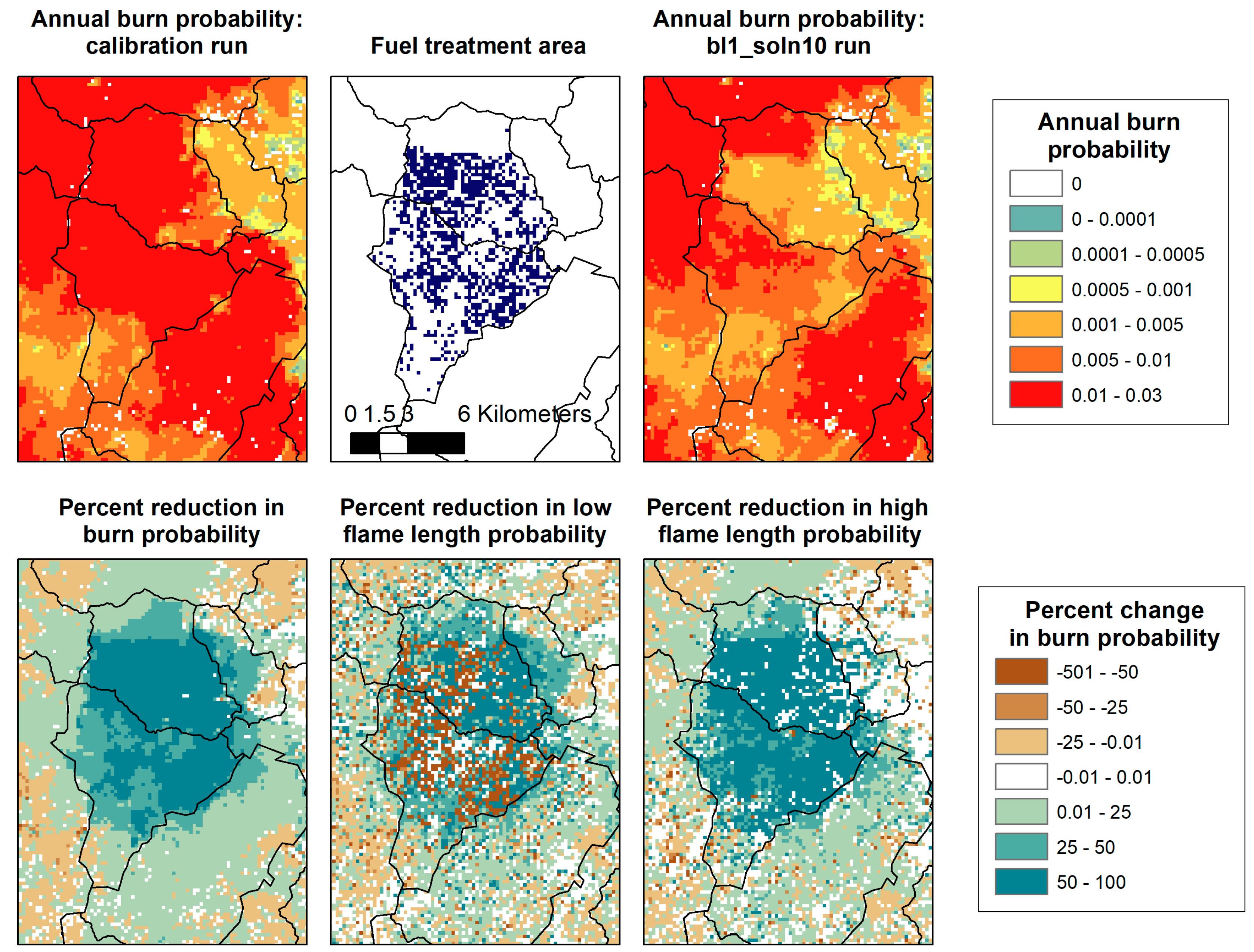
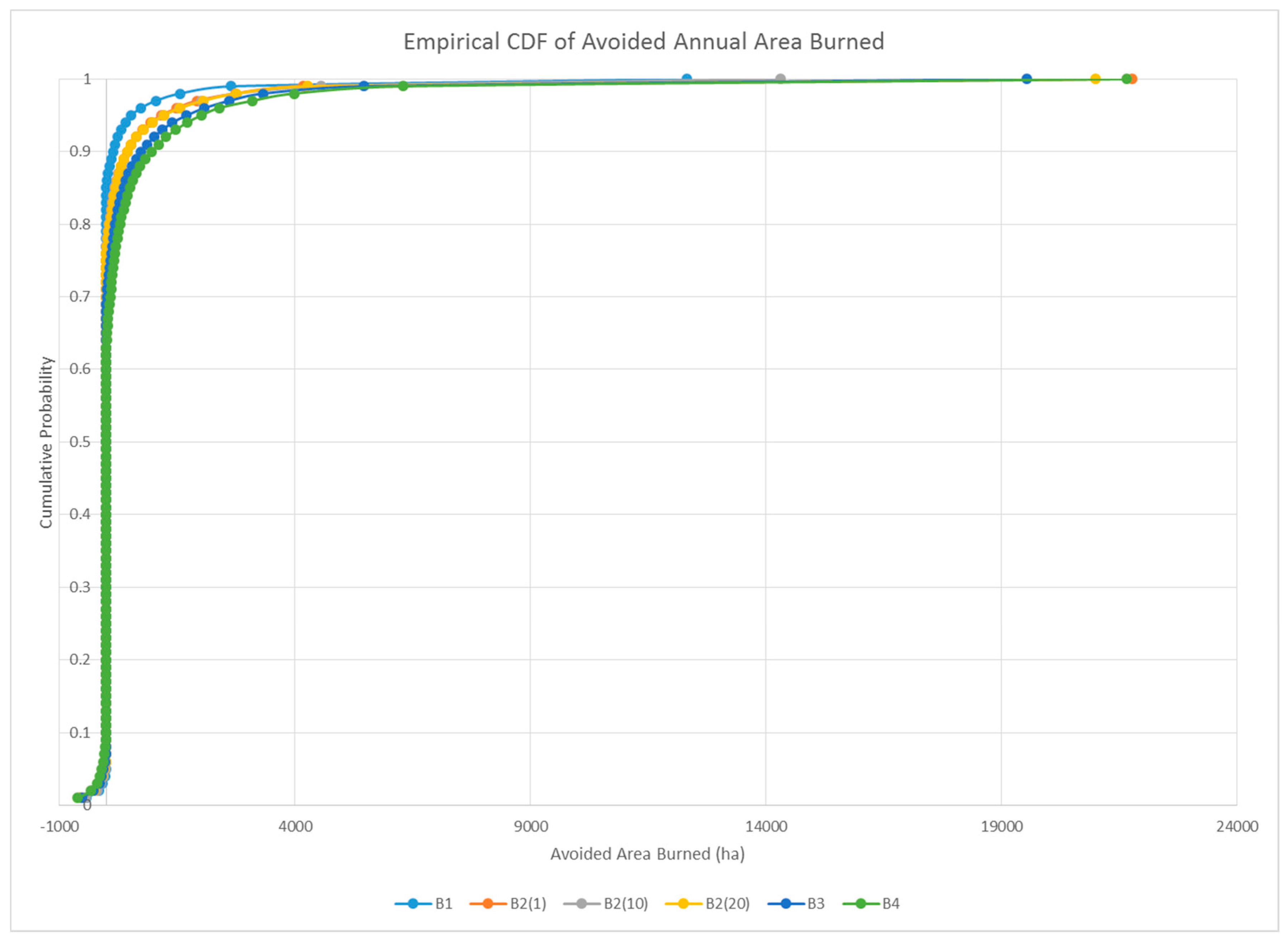
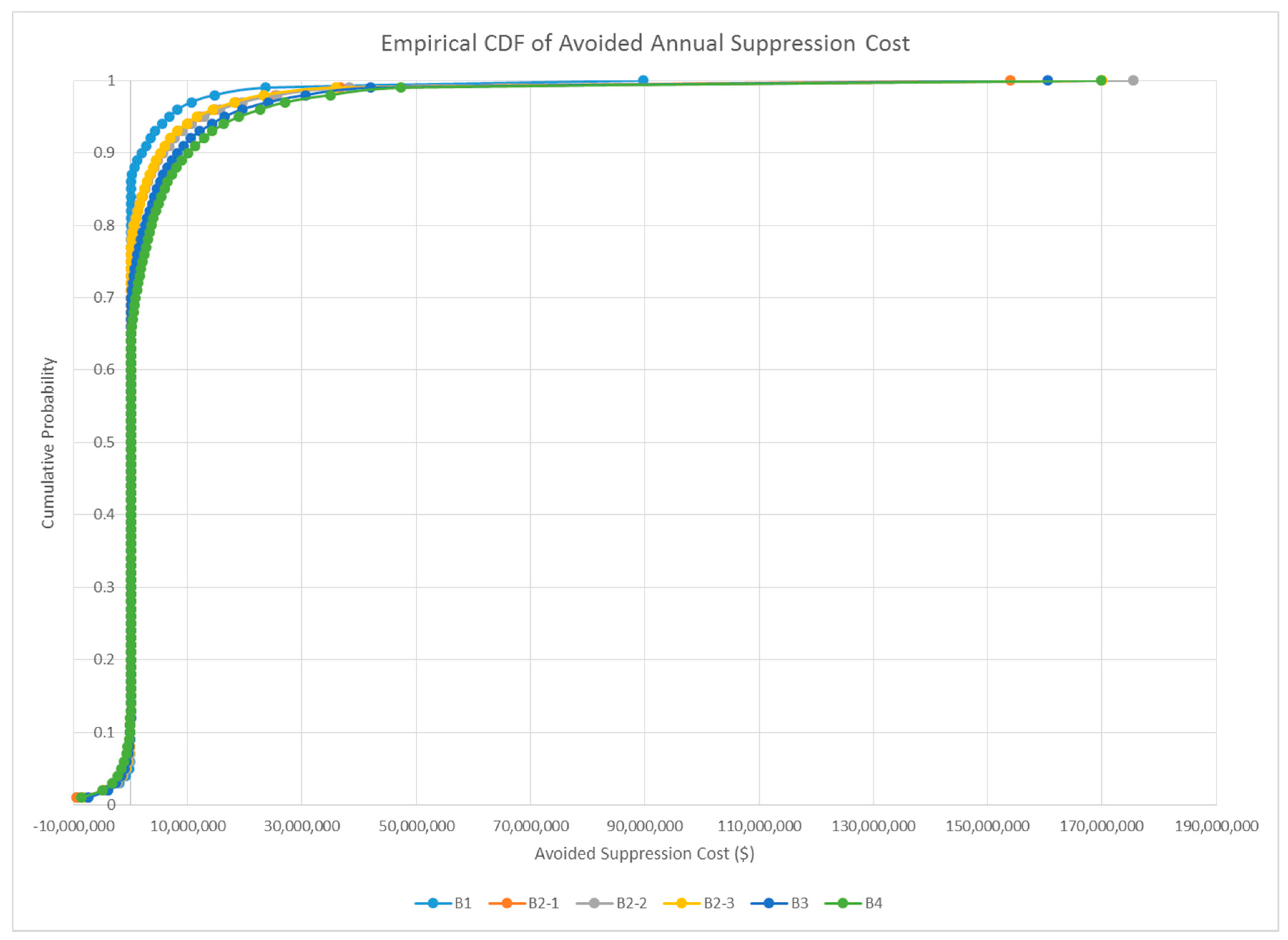
Table 1.
Summary of fuel treatment scenarios.
| Treatment Scenario | Number of PODs Treated | Area Treated (ha) | Percent of Sierra National Forest Treated | Percent Reduction in Sierra National Forest Mean Burn Probability |
|---|---|---|---|---|
| Budget 1 | 3 | 4031 | 0.7% | 3.7% |
| Budget 2 (1) 1 | 10 | 8217 | 1.4% | 6.8% |
| Budget 2 (10) | 7 | 7922 | 1.4% | 7.2% |
| Budget 2 (20) | 7 | 7919 | 1.4% | 6.7% |
| Budget 3 | 12 | 12,114 | 2.1% | 9.9% |
| Budget 4 | 24 | 16,534 | 2.9% | 12.0% |
1 Parenthetical number corresponds to solution number for budget level with multiple solutions selected.
Table 2.
Per-fire and annualized fire-treatment encounters; summarizing treated area burned.
| Budget 1 | Budget 2 (1) | Budget 2 (10) | Budget 2 (20) | Budget 3 | Budget 4 | |
|---|---|---|---|---|---|---|
| Mean annual number of large fires | 2.40 | 2.38 | 2.38 | 2.38 | 2.36 | 2.35 |
| Proportion of fires that encountered a treatment | 0.07 | 0.16 | 0.14 | 0.14 | 0.22 | 0.31 |
| Mean treated area burned per fire (ha) | 9.12 | 20.18 | 19.27 | 18.71 | 28.20 | 36.71 |
| Proportion of fire seasons where fires encountered a treatment | 0.15 | 0.28 | 0.24 | 0.25 | 0.34 | 0.42 |
| Mean annual treated area burned (ha) | 21.85 | 47.77 | 45.55 | 44.19 | 66.23 | 85.60 |
Table 3.
Avoided annual area burned summary.
| Budget 1 | Budget 2 (1) | Budget 2 (10) | Budget 2 (20) | Budget 3 | Budget 4 | |
|---|---|---|---|---|---|---|
| Mean reduction in annual area burned (ha) | 99.27 | 193.83 | 201.20 | 195.45 | 280.09 | 343.55 |
| Ratio of treated area burned to reduction in area burned | 11.23 | 10.03 | 10.91 | 10.93 | 10.45 | 9.92 |
Table 4.
Avoid annual suppression cost summary.
| Budget 1 | Budget 2 (1) | Budget 2 (10) | Budget 2 (20) | Budget 3 | Budget 4 | |
|---|---|---|---|---|---|---|
| Mean annual avoided suppression costs ($M) | 0.72 | 1.67 | 1.79 | 1.60 | 2.50 | 2.99 |
| Percentile corresponding to full offset of treatment cost | 0.97 | 0.97 | 0.97 | 0.98 | 0.98 | 0.98 |
| Payback period (years) | 13.82 | 12.01 | 11.16 | 12.50 | 12.01 | 13.36 |
| Treatment revenue (total) to fully offset treatment cost in 10 years ($M) | $2.76 | $3.35 | $2.07 | $4.00 | $5.02 | $10.06 |
| Treatment revenue ($/cubic meter) to fully offset treatment cost in 10 years | $27.85 | $18.83 | $9.86 | $18.05 | $17.74 | $28.74 |
Table 5.
Leverage metric summary.
| Budget 1 | Budget 2 (1) | Budget 2 (10) | Budget 2 (20) | Budget 3 | Budget 4 | |
|---|---|---|---|---|---|---|
| L(AB) | 0.06 | 0.06 | 0.06 | 0.06 | 0.06 | 0.05 |
| L($) | 0.07 | 0.08 | 0.09 | 0.08 | 0.08 | 0.07 |
| L(NVC) | 2.94 | 3.05 | 2.66 | 2.54 | 2.85 | 2.86 |
© 2017 by the authors. Licensee MDPI, Basel, Switzerland. This article is an open access article distributed under the terms and conditions of the Creative Commons Attribution (CC BY) license (http://creativecommons.org/licenses/by/4.0/).
Share and Cite
MDPI and ACS Style
Thompson, M.P.; Riley, K.L.; Loeffler, D.; Haas, J.R. Modeling Fuel Treatment Leverage: Encounter Rates, Risk Reduction, and Suppression Cost Impacts. Forests 2017, 8, 469. https://doi.org/10.3390/f8120469
AMA Style
Thompson MP, Riley KL, Loeffler D, Haas JR. Modeling Fuel Treatment Leverage: Encounter Rates, Risk Reduction, and Suppression Cost Impacts. Forests. 2017; 8(12):469. https://doi.org/10.3390/f8120469
Chicago/Turabian StyleThompson, Matthew P., Karin L. Riley, Dan Loeffler, and Jessica R. Haas. 2017. "Modeling Fuel Treatment Leverage: Encounter Rates, Risk Reduction, and Suppression Cost Impacts" Forests 8, no. 12: 469. https://doi.org/10.3390/f8120469
Note that from the first issue of 2016, this journal uses article numbers instead of page numbers. See further details here.