Suitability of Soil Erosion Models for the Evaluation of Bladed Skid Trail BMPs in the Southern Appalachians


Department of Forest Resources and Environmental Conservation, Virginia Polytechnic Institute and State University, 310 West Campus Drive, Blacksburg, VA 24061, USA
*
Author to whom correspondence should be addressed.
Forests 2017, 8(12), 482; https://doi.org/10.3390/f8120482
Submission received: 29 September 2017
/
Revised: 30 November 2017
/
Accepted: 30 November 2017
/
Published: 6 December 2017
(This article belongs to the Special Issue Forest Operations, Engineering and Management)
Abstract
:This project measured soil erosion rates from bladed skid trails in the mountains of Virginia following a timber harvest, and compared measured erosion to four erosion model predictions produced by Universal Soil Loss Equation—Forest (USLE-Forest), Revised Universal Soil Loss Equation, v.2 (RUSLE2), Water Erosion Prediction Project—Road (WEPP-Road) using default files, and WEPP-Road using modified files in order to assess the utility of the models for these conditions. Skid trails were segregated into six blocks where each block had similar trail slopes and soils. Each block contained four skid trail closure treatments: (1) bare soil (Control); (2) residual limbs and tops (Slash); (3) grass seed (Seed); and (4) fertilizer, seed, and straw mulch (Mulch). All treatments had waterbars, the minimum trail closure best management practice (BMP), to provide upslope and downslope borders of experimental units. Site cover characteristics on each experimental unit were collected quarterly as input parameters for erosion models. The suitability of soil erosion models were evaluated based upon statistical summaries, linear relationships with measured erosion rates, Nash-Sutcliffe Model Efficiency, and a nonparametric analysis. Treatments were measured to have erosion rates of 15.2 tonnes ha−1 year−1 (Control), 5.9 tonnes ha−1 year−1 (Seed), 1.1 tonnes ha−1 year−1 (Mulch), and 0.8 tonnes ha−1 year−1 (Slash). It was determined that WEPP-Road: Modified (p-value = 0.643) and USLE-Forest (p-value = 0.307) were the most suitable models given their accuracy; however USLE-Forest may be better for making management decisions given its practicality.
1. Introduction
The United States Environmental Protection Agency (USEPA) has identified sediment as the most damaging nonpoint-source pollutant in the U.S. [1]. Forest operations have the potential to produce substantial amounts of soil erosion that may be delivered as sediment in streams [2], thus a variety of forestry best management practices have been developed to either reduce soil erosion or interrupt delivery of eroded material to streams. In the southern Appalachians of the U.S., primary sources of soil erosion associated with forest operations are forest roads [3], overland [4] and bladed skid trails [5], and stream crossings [6]. Roads and skid trails are potentially highly erosive due to exposure of bare soil, terrain slope steepness, low road drainage standards [7,8], and traffic during poor weather conditions. The combination of these factors are known to increase erosion; therefore increasing the possibility of stream sedimentation and degradation [9,10]. Skid trails are potentially of more concern than haul roads because skid trails typically have lower standards than roads and skid trails may comprise a larger percentage of the harvest area [11]. Bladed skid trails are often used in the steep terrain of the region to facilitate skidder operator safety and operational efficiency. They differ from overland skid trails in that a bulldozer is used to construct the road, as opposed to having equipment simply drive on the surface of the soil [3,4]. Kochenderfer [12] estimated that up to 84% of exposed mineral soil in a harvest area was due to skid trails. More recently Worrell et al. [13] reported that bladed skid trails comprised approximately 8% of harvest area in the Appalachian Mountains. Wade et al. [5] measured erosion produced by bladed skid trails in the Piedmont region and determined that sediment production was strongly influenced by the application of forestry best management practices (BMPs). Trails with only waterbars produced 1.1 tonnes ha−1 year−1 of erosion whereas trails using slash or mulch cover produced <4 tonnes ha−1 year−1.
Best management practices for skid trails have been developed to reduce the impacts of forest operations on water quality [14]. Skid trail BMPs include pre-harvest planning (e.g., layout of bladed skid trails), water control structures (e.g., water bars), and the use of ground cover on skid trails [15]. Commonly suggested methods of ground cover for bladed skid trails include grass seed, straw mulch, and residual limbs and tops from the forest harvest (slash) [16,17,18,19]. These methods of ground cover have been found to be both effective and economical in the past [4,5,20].
Soil erosion has the potential to reduce site productivity [21,22] and negatively impact water quality [2], thus quantification of the effects of forest best management practices on soil erosion are clearly important. However, on-site measurement of erosion is often costly and time consuming, thus models are commonly used to estimate erosion potentials [23,24]. Several models were developed to allow agricultural land managers to estimate and prioritize erosion issues and have been adapted to forest use over time [25]. Erosion models can be used by forest managers to make silvicultural, management, or even forest engineering decisions [26]. They are frequently modified to maintain and increase their accuracy and dependability [23]. One of the oldest and most widely applied soil erosion models is the Universal Soil Loss Equation (USLE) that was originally developed by the USDA in 1954 to estimate potential sheet and rill erosion from agricultural lands. The USLE is an empirical model that has been adapted to predict erosion from rangelands, minelands, watershed, and forest lands [27]. Dissmeyer and Foster [28] modified the USLE for use on forestlands (USLE-Forest). The USLE-Forest is relatively simple to use and has been widely used successfully on skid trails in the Piedmont physiographic region [4,5,20]. The USLE-Forest equation components are:
where A is the annual soil loss per unit area, R is the rainfall and runoff factor, K is the soil erodibility factor, L represents the slope-length factor, S is the slope-steepness factor, C is the cover and management factor, and P represents the support practices factor [28]. R is determined based upon the average weather conditions at the location of interest. K is a function of multiple soil characteristics: soil texture, organic matter content, structure, and permeability. K values can be found in soil surveys or soil descriptions [29]. More accurate K-value estimates can be obtained by completing a nomograph included in the USLE-Forest manual. The L value is “the ratio of soil loss from the field slope length to that from a 72.6-foot (22.13 m) length under identical conditions” [28]. Likewise, slope-steepness factor (S) is defined as “the ratio of soil loss from the field slope gradient to that from a 9-percent slope under otherwise identical conditions” [28]. These two variables can be determined from a table found in A Guide to Predicting Sheet and Rill Erosion on Forest Land, written by Dissmeyer and Foster [28]. Cover and management (CP) factors are based upon the amount of bare soil, presence of canopy, soil reconsolidation, high organic matter content, fine roots, residual binding effects, onsite storage, and natural sediment trapping resulting in steps, and can be derived from tables published by Dissmeyer and Foster [28].
A = RKLSCP
The USLE was later revised and converted to a computerized format, labeled the RUSLE or Revised Universal Soil Loss Equation. This model was first produced in the early 1990’s, and RUSLE1.06 and RUSLE2 were both released in 2003. Although the original empirical algorithm from the USLE was kept, it was modified for improved accuracy by deriving soil loss factors in new ways. This revision included changes to make the model more suited for use with forest lands. Other improvements included updated rainfall coefficients, after changing some of the R factors in the eastern US based on weather data collected from more than 1200 weather stations. Soil erodibility (K) is varied seasonally for increased accuracy. The LS factor is improved in that it takes into account the “susceptibility of the soil to rill erosion relative to interrill erosion” and the cover factor uses a new algorithm for determining cover based on prior land use, canopy cover, soil cover, and soil surface roughness [30]. RUSLE2 has no specific data files for forest roads, however there are “highly disturbed land” files that can be modified to suit different forest road treatments [24].
The Water Erosion Prediction Project (WEPP) is a physically-based model produced by the U.S. Department of Agriculture Natural Resource Conservation Service (NRCS) and U.S. Forest Service (USFS) to replace the USLE formula. WEPP “models soil erosion as a process of rill and interrill detachment and transport” [31] as opposed to empirically modeling the ground conditions [32,33]. The WEPP model had additional potential utility because it estimates daily conditions that affect erosion, over the course of a year. In this, senescence, plant growth, residue accumulation and decomposition, as well as daily temperatures and soil water availability are taken into account to provide a very detailed estimate of soil loss over time. An additional benefit is the ability to model complex slopes and forest road profiles, with features such as cutslopes and fillslopes, ditches, and road surfaces [23]. Four types of data files are required to run WEPP: (1) a climate file, to include data on daily precipitation and temperature; (2) a hillslope file, which can contain multiple points to describe a slope’s shape; (3) a soils file, which can include multiple soil types across the hillslope; and (4) a management file containing information on soil disturbances and vegetative conditions present [26]. Weather data are obtained through Cligen, the USDA’s weather resource. This weather file models weather data on a daily basis for more than 1000 climates [34]. Using the hillslope file, WEPP determines the erosion or deposition rates for at least 100 points of the hillslope if there is any runoff predicted that day [35]. Because WEPP, like other models, was originally intended for cropland or rangelands, there have been many efforts to adapt it for forest uses [36,37,38,39,40,41]. One of these interfaces is the WEPP-Road model interface. This program allows the user to determine the amount of sediment delivered to the stream through the forest buffer and amount of sediment eroded from each portion of the road, as well as determine the presence of a sediment plume in the forest [42]. At this time, the selections for cover and land use scenarios appear to limit WEPPs utility for estimation of erosion for many eastern forest management regimes [43].
There have been several attempts to assess the performance of these three models. Wade et al. [24], compared sediment trap data to predictions by all three models. Erosion rates were estimated from different sections of bladed skid trail in the Piedmont of Virginia using sediment traps, and were then compared to erosion rates predicted by USLE, RUSLE2, and WEPP models. It was found that overall, all three models performed well enough for identifying erosion hazards and making management decisions. When comparing the modeled data, it was determined that USLE-Forest ranged from 0.9× to 2.2× the actual erosion rates from data collected from the sediment traps. RUSLE2 ranged from 0.4× to 2× the actual erosion, and WEPP-Road ranged from 2.3× to 7.5× [24]. These data indicated that the USLE-Forest and RUSLE2 can be useful at approximating erosion rates, but WEPP-Road values should only be used for ranking purposes on bladed skid trails. Foster, Toy, and Renard [44] found similar results when comparing USLE, RUSLE1.06, and RUSLE2. WEPP modeling efforts can be improved with laborious programming, but is time consuming and requires many measurements to modify the working files [45]. Lang et al. [45] found that soil erosion models worked best when estimating erosion rates less than 11.2 Mg ha−1 year−1; however when erosion rates surpassed this amount model estimates varied widely. Croke and Netherly [25] compared the USLE and WEPP on skid trails in Australia and concluded that the USLE was more user friendly while the WEPP model was a better predictor of erosion on skid trails. However, their investigation indicated that neither method was wholly satisfactory for estimation of erosion. One important distinction to note is the difference between empirical models, which are simpler to use but are based on observations and measurements; and physically-based models which replicate erosion processes as equations [32,33]. Both types of models have their own advantages and applications [32].
Overall, the literature clearly indicates that erosion from skid trails can be a significant source of nonpoint source pollution from forestry operations [2,46,47,48] and that rates of erosion for different types of skid trail BMPs are warranted in order to evaluate BMP efficacy. This aspect of the problem is addressed by a companion paper [49]. Furthermore, the literature indicates that erosion models have been used with varying success to estimate erosion from skid trails, but modeled erosion rates from bladed skid trails in mountainous terrain have not been compared to direct erosion measures.
The primary objective of this study was to compare measured erosion rates from four bladed skid trail closure methods in mountainous terrain with those produced by the Universal Soil Loss Equation (USLE-Forest), the Revised Universal Soil Loss Equation (RUSLE2), the Water Erosion Prediction Project (WEPP-Road: Default), and a more modified version of WEPP (WEPP-Road: Modified).
2. Materials and Methods
2.1. Research Site
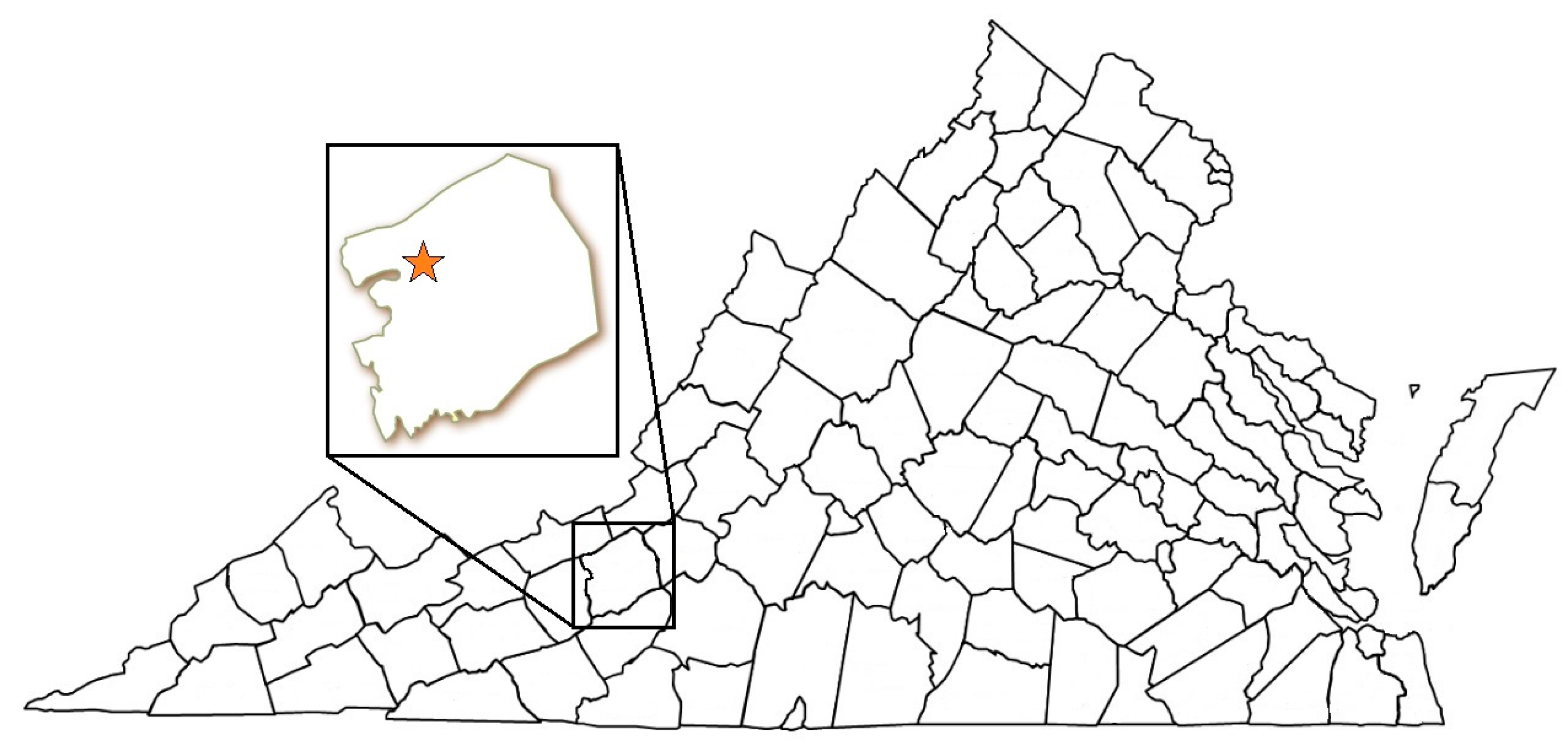
The study site is located in the Ridge and Valley physiographic province, on Virginia Tech’s Fishburn Forest located in Montgomery County, Virginia (Figure 1). This physiographic province is characterized by long mountain ridges with constant linear valleys in between them. The average yearly precipitation is 103.86 cm [50]. The average high and low temperatures for this location in January are 5.3 °C and −5.9 °C. The average high and low temperatures in July are 27.9 °C and 15.6 °C [50]. Rainfall data were collected from a nearby weather station for the duration of the study period (Figure 2) [51] and were used to compare the effects of rainfall on erosion rates [49].
The soils are very shallow, well drained silt loams, being derived mostly from shale, siltstone, and sandstone residuum. Berks, Weikert, Berks-Weikert and Clymer soil series (Lithic Dystrudepts) dominate the site [29]. The harvested stands were primarily mixed upland hardwood-pine stands, composed of white pine (Pinus strobus L.), chestnut oak (Quercus montana Willd.), and white oak (Quercus alba L.). Slopes in this region range from 0% to 100%.
The site was harvested in late 2014-early 2015 using a shelterwood overstory removal of upland hardwoods and pine. Skid trails were laid out in a “logger’s choice” arrangement. Skid trail slopes ranged from 0–35%, with an average slope of 16%. Skid trail sideslopes ranged from 5–45%. The skid trails were divided into 6 blocks based on slope class. Two blocks were arranged in each slope class: Gentle (0–10%), Moderate (11–20%), and Steep (>20%). Each block of treatments contained the four closure methods that were compared in this experiment.
Treatments consisted of 15.2 m segments of skid trail, approximately 2 m wide. On steep slopes (>20%) the treatments were shortened to 12.2 m in order to comply with state BMP guidelines [14]. Closure methods were randomly assigned to each of the 24 experimental units. Units were separated by waterbars. Skid trail treatments were closed to vehicle traffic over the course of the study period in order to avoid any effects of heavy trafficking on soil erosion rates [52].
2.2. BMP Treatments
Four types of treatments were used in this study: (1) waterbars only (Control), (2) waterbars with grass seed (Seed), (3) waterbars with grass seed, fertilizer, and straw mulch (Mulch), and (4) waterbars with slash (Slash) (Figure 3). The Control treatment consists of waterbars with no ground cover treatments and represents the minimum acceptable BMPs as a control reference to which the other treatments were compared. For the Seed treatment, grass seed was applied at the time of skid trail closeout (April 2015) using a mix of 50% perennial ryegrass (Lolium perenne L.) seed and 50% K-31 fescue (Festuca arundinacea Schreb.), based on suggestions from the VDOF BMP manual [14]. Seeds were spread with a hand operated seeder to ensure adequate coverage, at a rate of approximately 168 kg/ha. For the Mulch treatment, the same grass seed mixture was applied, followed by fertilizer and straw mulch. Mulch was spread by hand to ensure near total coverage, at a depth of 3–6 cm across each experimental unit [14]. Fertilizer [5-10-10 (N, P2O5, K2O)] was added at a rate of 336 kg/ha to provide sufficient nutrient availability for the grass. Slash treatments utilized residual slash from on-site logging operations, and was primarily composed of yellow-poplar (Liriodendron tulipifera L.), hickory (Carya spp.), scarlet oak (Quercus coccinea Münch.), chestnut oak (Quercus montana Willd.), white oak (Quercus alba L.), white pine (Pinus strobus L.), and Virginia pine (Pinus virginiana Mill.). Slash was hand applied onto skid trails to ensure similar coverage and then compacted with a bulldozer to make contact with the ground. After being tracked in by the bulldozer, slash was at a depth of 0.6–0.9 m.
2.3. Sediment Trap Installation and Measurement
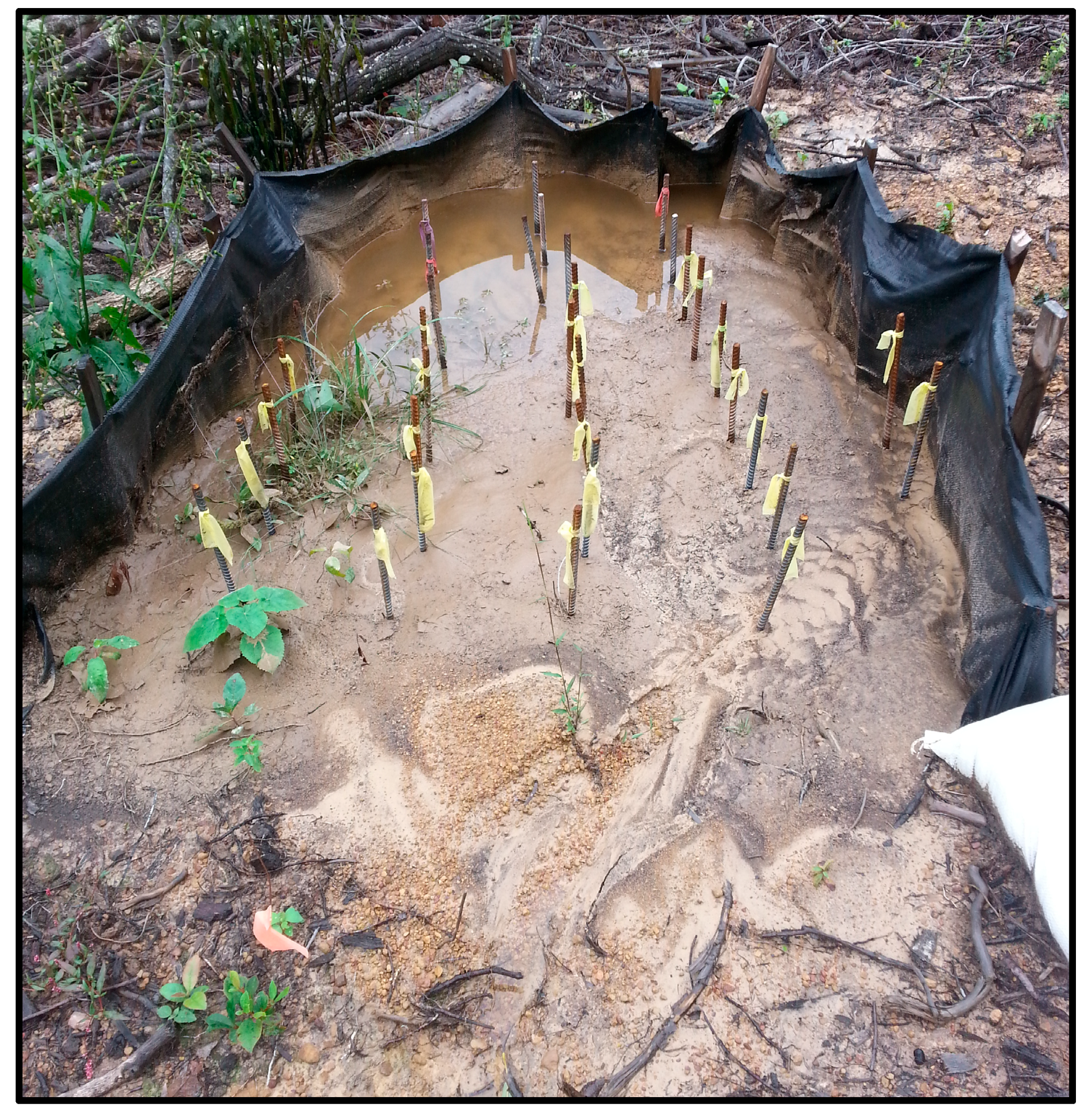
A full description of the collection of field data and the effectiveness of skid trail closure methods is available from Vinson et al. [49]. Sediment traps were used to measure erosion rates in the field over the course of the year. These sediment traps consisted of silt fences that were joined to the downslope waterbars so that they collected all runoff from the skid trail treatment (Figure 4). Berms were constructed on either side of the skid trail to limit overland flow and to ensure runoff from the treatment made it into the sediment trap. Within each sediment trap, metal pins were driven into the ground at regular intervals in a grid pattern. The depth of the sediment was measured at each sediment pin on a monthly basis, as was the area of the sediment collected. From this a volumetric accumulation of sediment was determined over time. Bulk density samples were taken from the accumulated sediment, and this was used to convert the volume of collected sediment to a gravimetric amount.
2.4. Erosion Model Parameters
For modeling, each experimental unit was divided into three sections. The first section being the downhill side of the upslope waterbar, the second section being the actual skid trail surface, and the third being the uphill side of the downslope waterbar (Figure 5a,b). Section 1 and Section 2 were modeled together. Since the two waterbars have sides that are contributing to the area, they needed to be accounted for in the modeling as well. The slope and length of every section was measured using a total station. The USLE was used to estimate erosion from each section of each treatment, and estimates were combined in a weighted average total erosion estimate for each treatment. Grass treatments had model estimates determined both before and after seed germination for a comparison, as ground cover values were measured in the field every 3 months to account for variations in seasons, the establishment of grass, and decomposition of slash and mulch. Slope, climate data, soil characteristics, and cover practices were determined for each experimental unit and input into all three models to estimate soil loss. Actual erosion rates were converted to tonnes ha−1 year−1 in order to compare estimates provided by all three models. For each treatment area the following data were collected: ground cover, slope gradient and slope length, percent of soil in clay, sand, and silt, soil rock content, and rainfall data.
2.5. USLE-Forest Parameters
A rainfall runoff factor of 150 was used as it was derived from a rainfall contour map provided by the USLE-Forest manual [28]. A soil erodibility factor of 0.43 was obtained from the Montgomery County, VA Soil Survey [29]. A total station was used to measure the slope length and gradient for the upper and lower waterbars, and the section of bladed skid trail located between the two. Slope lengths were often too small to be found in the USLE-Forest manual, and therefore were obtained using the equation:
where λ is the slope length in feet, θ is the slope angle in degrees, and m is 0.2 for <1% slopes, 0.3 for 1% to 3% slopes, 0.4 for 3.5% to 4.5% slopes, and 0.5 for ≥5% slopes [28]. The bladed skid trails were considered to be tilled soil, therefore having CP factors to include bare soil, residual binding, and soil reconsolidation; canopy effect; steps; onsite storage; invading vegetation; and contour tillage. Bare soil percentages were calculated by creating transects across the treatment, with evenly spaced points. At each point, ground cover was determined to be either bare or covered, and ground cover percentage was calculated. Ground cover included vegetation, straw mulch, woody residues, rock fragments, and leaf litter. These measurements were collected quarterly over the course of a year to cover the span of four seasons. A weighted average of the four periods was used to determine a final annual erosion rate for each treatment.
LS = (λ/72.6)m(65.41sinθ2 + 4.65sinθ + 0.065)
2.6. RUSLE Parameters
Erosion estimates were also predicted using RUSLE2. Montgomery county weather and soil files were imported into the program to more accurately estimate soil loss. Climatic data were accessed from the NRCS database [29] for Montgomery County, Virginia. Daily and monthly average rainfall rates were included in these data. Montgomery county soil survey indicated the Berks-Weikert complex as the soil series for the site [29], the soil file for which was then imported into the program. The soil file contains information on the erodibility of the soil, the soil texture, and acceptable loss rates. For every treatment, a slope profile was created based on the measured slope and length of each section of the treatment area. Management files had to be created for each BMP treatment, as there were no pre-made files to represent forest roads or skid trails. All operations were set to occur in late April to coincide with the initial site installation. The “highly disturbed land/blade cut” option was selected to represent the Control treatments. Seed treatments used this file, but with the modification of “broadcast seed operation” also used. “Fescue” and “Ryegrass” were used as the species of seed applied, and the “live surface cover” was modified to represent the percentage of ground cover contributed by the germination of the grass seed as time increased. Mulch treatments used this file; however it was modified to include the “add mulch” operation in the form of “bale straw or residue.” The type of mulch chosen in this instance was “wheat straw.” The option “specify cover directly” was chosen and modified for each treatment to correspond with cover percentages measured in the field. Slash treatments were best represented by the “highly disturbed/blade cut” option, followed by the “add mulch” operation, with “prunings, orchard and vineyard, flail shredded” chosen as the material. The cover was again manipulated by modifying the “specify cover directly” parameter, and by modifying the decomposition half-life of the material to 1800 days, as based on rates used by Wade et al. [24] to represent the decomposition rate of woody debris from southern Appalachian hardwood forests.
2.7. WEPP-Road: Default Parameters
WEPP-Road is dependent upon four different types of files to predict soil erosion rates. The software features a database that contains basic files for each of these that can be easily modified to best represent the site. The four types of files are: (1) climate; (2) soil characteristics; (3) slope length and gradient; and (4) land management operations. A climate file for Blacksburg, Virginia is embedded into the software and was therefore chosen as the best representative of the site conditions, as the weather station is less than 8 km (5 miles) away from the study site. Within the WEPP-Road soils database, the file most similar to a Berks-Weikert complex was the “Disturbed Skid Clay Loam,” which was chosen for modeling on this site. Soil rock content for each treatment varied from 10–36%, and was directly correlated with slope steepness. Therefore, it was determined that rock content of the soil would be a parameter which needed modification for each treatment, as well as factored into the ground cover in the initial conditions and management files. Slope length and gradient values were modified for each treatment as they were measured with the total station. The “Forest Bladed Road” management file was used for the Control treatments, and was modified for the others. Initial conditions were modified by their initial rill and interrill ground cover percentage, as measured in the field. Seed treatments used this base of “Forest Bladed Road” as the initial conditions and then were modified with the “fescue” and “annual ryegrass at a low fertilization rate.” Mulch treatment management files used this file as a base, however “fescue residue” was added as a mulch at a rate of 0.788 kg m−2. Similar to RUSLE2, there are no management files in WEPP-Road that represent Slash treatments. Since there are no woody residue mulch treatments, the same “fescue residue” mulch was chosen. The actual application rate (by weight) that was used to apply slash in the field was used to model this treatment, similar to methods used by Wade et al. [24]. All treatments were modeled for one year.
2.8. WEPP-Road: Modified Parameters
WEPP-Road was then used to model these treatments a second time, using files that were modified to more accurately represent the soil and treatment conditions throughout the year. The primary reason for this being that WEPP-Road has a large number of parameters that can be manipulated when using the model. We wished to determine if collecting more data and making use of more of the model parameters would provide a significantly more accurate soil erosion estimate, and how much more labor would be needed to accomplish this. A soils file was created for each experimental unit based on the “Disturbed Skid Clay-Loam” file used earlier, but modified with the soil rock content and soil particle size present in each of the experimental units. The model was used to calculate interrill erodibility, rill erodibility, critical shear, and effective hydrologic conductivity instead of using the default preset values in place for that particular file. The weather file remained the same, as the Blacksburg, Virginia climate file was determined to be accurately representative of the study site based on its geographic proximity. Slope gradient and length were created once again based on measurements taken in the field with a total station. For the Control treatment, the same “Forest Bladed Road” management file was used for the control treatments, and was modified for the others. The Forest Bladed Road file was modified with initial rill and interrill ground cover percentage, as well as bulk density of the experimental units. This time, the “Initial Plant” field in the “Initial Conditions” file was changed to “Skid Trail-Disturbed,” and the “Days Since Last Tillage” field was modified to reflect that the disturbance had just occurred (0 days). Seed treatments used this base of “Forest Bladed Road” as the initial conditions and then were modified with the “fescue” and “annual ryegrass at a low fertilization rate.” Mulch treatment management files used this file as a base, however “annual ryegrass at a high fertilization rate” was used instead of “annual ryegrass at a low fertilization rate;” and “fescue residue” was added as a mulch at a rate of 0.788 kg m−2. Once again, there are no files in WEPP-Road that represent woody material for Slash treatments. In this instance, the “Rock” file was chosen in the “Residue Added” field, and was modified to represent the decomposition rate of woody material. This file was chosen because it is the closest available file that could be modified to represent a slash treatment. The actual application rate (by weight) that was used to apply slash in the field was used to model this treatment. All treatments were modeled for one year.
2.9. Data Analysis
Treatment effects for each erosion model were analyzed using JMP statistical software [53]. A variety of methods were used to compare the trapped and modeled estimates including: (1) summary statistics; (2) linear relationships; (3) Nash-Sutcliffe Model Efficiency (NSE) [54]; and (4) a nonparametric analysis. Summary statistics were analyzed to examine means and standard deviations for each treatment using each erosion model. Linear relationships, and NSE were evaluated to determine the accuracy of the models when compared to the actual trapped erosion rates, and a nonparametric comparison for each pair using the Wilcoxon method was conducted to compare these models to each other. Similar comparisons have been conducted by Wade et al. [24] and Croke and Netherly [25].
3. Results
3.1. BMP Treatment Effectiveness
The sediment collected in traps clearly indicates an overall effectiveness of the BMPs compared. Control treatments with waterbars only were measured to have an erosion rate of 15.2 tonnes ha−1 year−1. Seed treatments were measured to have an erosion rate of 5.9 tonnes ha−1 year−1, and Mulch treatments eroded at a rate of 1.1 tonnes ha−1 year−1. Slash treatments eroded at a rate of 0.8 tonnes ha−1 year−1. Each model ranked the BMP treatments as having the Control as the most erosive, and the Mulch treatment as least erosive. All models tended to over-estimate the erosion rates of Slash treatments. The Control treatments represent the minimum level of BMPs that are acceptable for skid trail closeout, and was measured to have eroded at rates 2.8× to 8× that of seeded treatments, the next most erodible treatment [49]. Mulch and Slash treatments both reduced average sediment rates to minimal amounts. Adding mulch and fertilizer provided the trail with immediate ground cover, which was not attained by the Seed treatments due to the time necessary for germination. Mulch also aided in the retention of soil nutrients and moisture, as well as reduced predation of the grass seeds from wildlife. Slash provided immediate ground cover, and offers the additional benefits of reducing traffic on the trail, in the form of four-wheelers and pedestrians. After cost analysis, Slash was also shown to provide the greatest benefit in soil erosion reduction per dollar spent in installation [49]. This is due to the fact that no materials are needed to be purchased to install a slash treatment, since slash is already present following the harvest. For all treatments, as ground cover increased, soil erosion decreased. Slope and length did have effects upon the erosion rates, as did rock content of the soil. Steeper slopes in this soil series tended to feature higher rock fragment contents, which acted to increase soil cover over time as the soil around them was eroded away. More information on BMP effectiveness and erosion rates over time may be found in Vinson et al. [49].
3.2. Model Suitability
Models were evaluated using the four different techniques outlined earlier. Each of the model predictions was compared to the trapped sediment data after one year (Table 1). WEPP-Road: Modified had the closest overall mean erosion rate estimate for the Control treatments, while RUSLE2 had the closest overall mean erosion rate for the Seed and Mulch treatments and USLE-Forest provided the closest overall mean erosion rate for the Slash treatments. It is to be noted that for the Control and Slash treatments, the estimates provided by RUSLE2 were more than double the next closest estimate, indicating that its results may be very inconsistent based on the conditions being modeled.
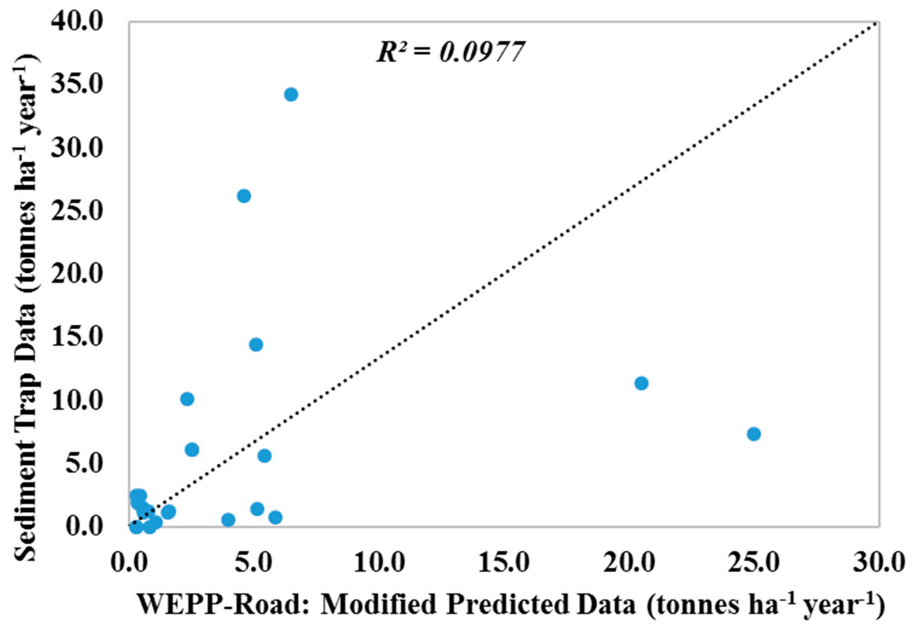
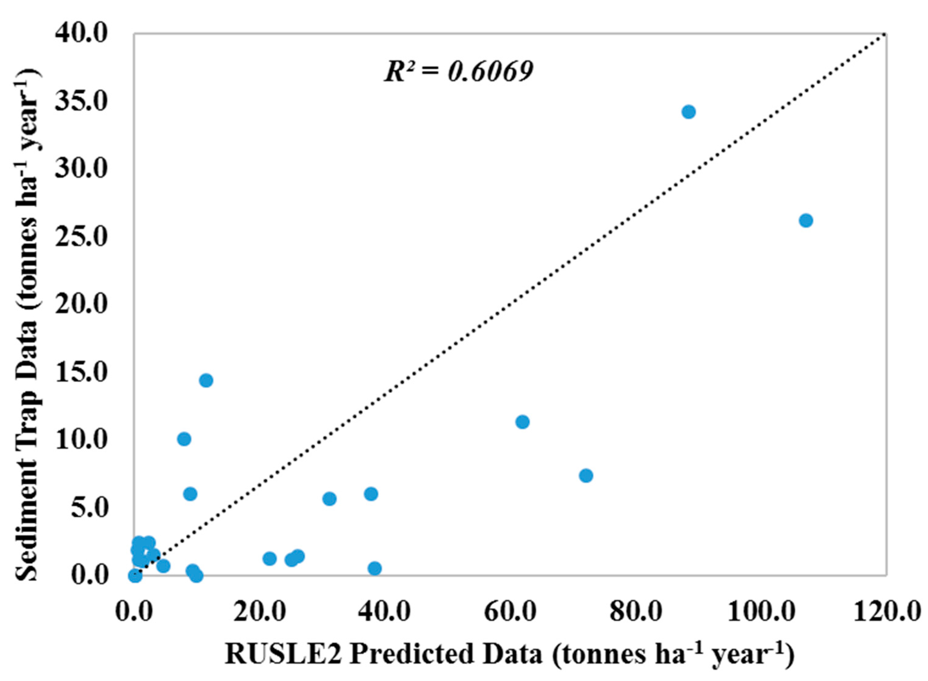
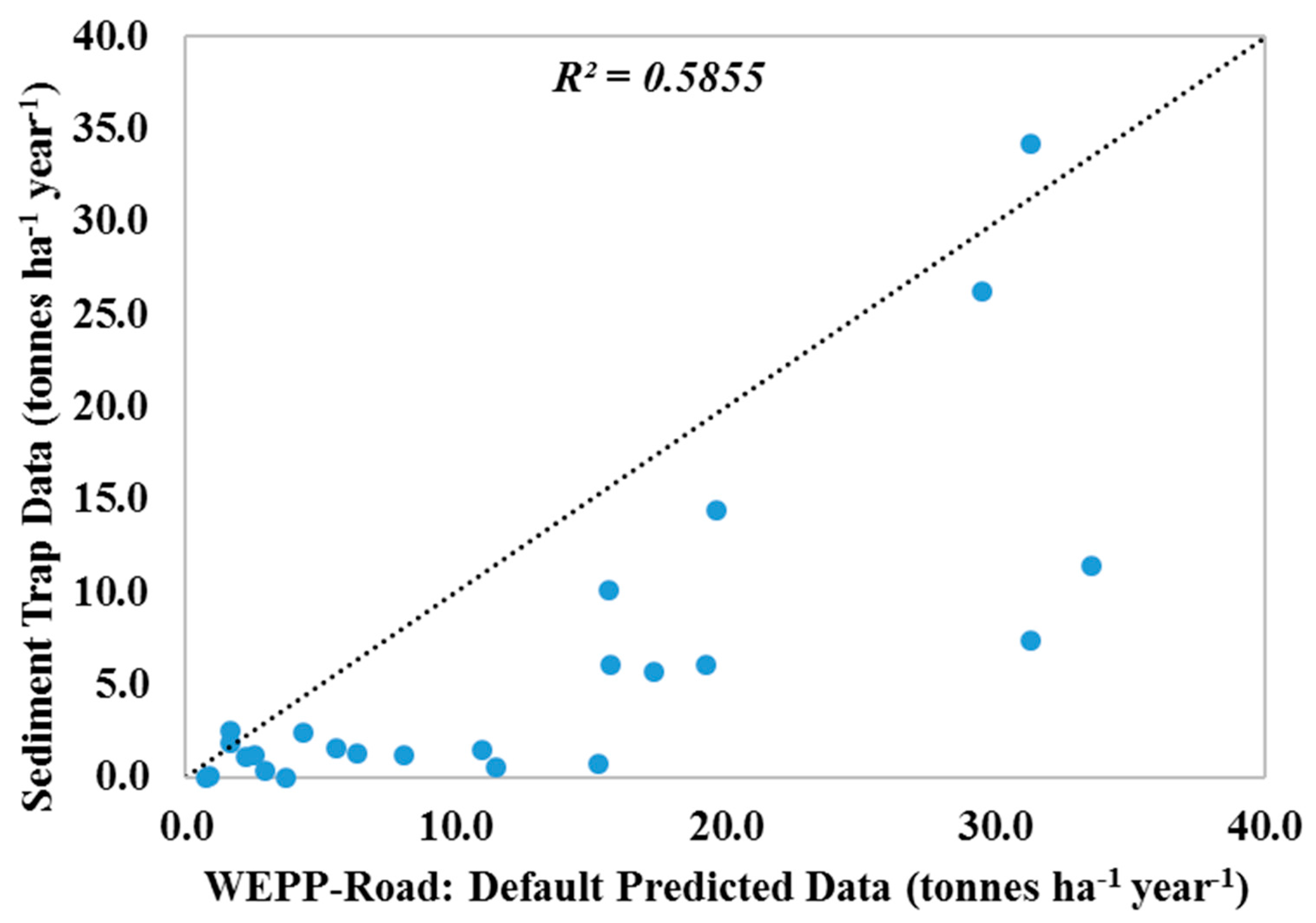
Linear relationships were also used to determine model accuracy. Each of the sets of modeled data were compared to the data collected by sediment traps. Accurate models are expected to have a linear relationship to the collected data [24]. In this study, RUSLE2 was shown to have the highest R2 value amongst the three, at 0.6069 (Figure 6). This indicates that RUSLE2 has the best estimated linear relationship with the trapped data. The linear relationship of WEPP-Road: Default to measured data has the second highest R2 value of 0.5855 (Figure 7), followed by USLE-Forest with an R2 value of 0.4652 (Figure 8). When compared to the 1:1 line, the inclination of the trend lines of these models indicate that they both tend to overestimate erosion rates. Lastly, the relationship of WEPP-Road: Modified to the measured erosion data has the lowest R2 value (0.0977) which is indicative of a poor model accuracy (Figure 9). This could have occurred due to inadequacies in modeling just one specific treatment.
The Nash-Sutcliffe Model Efficiency (NSE) is commonly used to evaluate hydrologic models. The range of efficiency is from −∞ to 1, with values from 0–1 indicating that the model is a good predictor of the measured values. As values approach 1, the model is a more accurate representation of true values. Negative values indicate that the mean of the measured values are a better predictor than the model itself [54], with lower values representing less suitable models. NSE was calculated for each of the treatments and each of the models as a whole (Table 2). All values were negative with the exception of the WEPP-Road: Default (0.15) and RUSLE2 (0.23) models at predicting Mulch treatment erosion rates. The NSE values for the other two models are negative for this treatment (−0.29, and −0.24), however they are substantially greater in value than most other treatment categories. This is evidence that the models did reasonably well at predicting erosion from Mulch treatments. Control treatments were found to have the lowest values for each model, indicating that all models were insufficient at predicting soil loss from bare soil treatments. When evaluating the entire model over all types of treatments, RUSLE2 has a much lower NSE value (−1174.15) than USLE-Forest (−146.35), WEPP-Road: Default (−115.01), and WEPP-Road: Modified (−102.72) indicating that it is the least suitable of the three models. Using this “whole model evaluation,” WEPP-Road: Modified has the highest NSE score and would be ranked the most accurate of the four.
Lastly, the models were analyzed using a nonparametric comparison for each pair using the Wilcoxon method (Table 3). For this method, each model was individually compared to the measured data to find significance. In this instance, WEPP-Road: Default and RUSLE2 were considered to be significantly different to the measured data (p-value = 0.0046, p-value = 0.0154).
4. Discussion
Results indicate that the BMPs effectively provided ground cover necessary to reduce erosion. Generally, as ground cover increased, erosion rates decreased. It was seen in the field that rock fragments had a major impact on ground cover and therefore erosion rates [49], which may have been difficult for the models to assess. Slash, seed, and straw mulch have been shown to reduce erosion from skid trails and temporary roads. Slash and straw mulch both provide immediate cover, especially during the initial months at which one can expect erosion rates to be the highest. Slash is readily available, lasts longer than straw mulch, and is more effective at reducing trail traffic. Both slash and straw mulch may also improve the chemical and physical properties of the soil through decomposition. This study indicates that additional road closure BMPs can be used to enhance the minimal effects of waterbars only. Erosion models were shown to have varying degrees of accuracy and suitability based upon their use. Similar conclusions were also reached by Wade et al. [24], Brown et al. [43], and Lang et al. [45].
USLE-Forest was slightly different than the other models in terms of management and cover practices. Whereas RUSLE2 and WEPP-Road model a specific operation and make assumptions based upon its effects, USLE-Forest models these effects directly. This has a noticeable impact on the accuracy of the model. However, many field measurements are required to produce a feasible value from this model. Soils, ground cover, and canopy cover must all be measured in the field. However, this does allow for a more “field available” prediction, whereas RUSLE2 and WEPP-Road both require the use of computer software. The USLE was shown to be the most user-friendly of the three models, in that it can easily be performed with a manual in the field with relatively minimal training and still provide an acceptable estimate of soil loss. Of all the models compared, USLE-Forest provided a consistently, reasonably reliable prediction with minimal difficulty.
RUSLE2 was determined to be the least suitable of the four models assessed, in that its NSE values and nonparametric p-values are all the least favorable of the models. One of the factors affecting the model accuracy is the aforementioned soil rock content. While soils files were accurate enough for the model, it did not take into account the increased soil ground cover from the high soil rock content over time. Other factors include the fact that operations are modeled as such instead of the effects that those operations had upon the ground surface [44]. The primary reason for poor performance of this model would be the fact that there are no management files available for bladed roads or slash treatments. However, RUSLE2 was able to model Seed and Mulch treatments exceptionally well. This shows that RUSLE2 can sufficiently model soil loss for certain ground conditions, but overall may be too inconsistent to be trusted.
WEPP-Road (both Default and Modified) was shown to be the most accurate of the four models based on NSE. This can be attributed to a number of factors. This is the only model that takes into account soil rock content in its analysis, which could have helped to make predictions more accurately. In addition to this, there are forest road and skid trail treatment files available, which gives WEPP-Road an advantage over RUSLE2. One major disadvantage to WEPP is that it does not feature any wood or wood-fiber based mulches to represent slash treatments. Both WEPP-Road and RUSLE2 are at a disadvantage, in that when compared to USLE-Forest, they are difficult to learn initially. They also require significant computer use, which is not always practical for field management decisions.
WEPP-Road: Modified outperformed WEPP-Road: Default. Of the predictions that the modified WEPP model produced, 71% were closer to the measured value than the default WEPP predictions. Lang et al. [45] found similar results when comparing soil erosion models to trapped data from forest haul roads. However, there were some treatments that WEPP-Road: Default modeled better than WEPP-Road: Modified. Inaccuracies in the modified version may have arisen from issues with certain parameters, resulting in the low correlation of modeled points in a linear relationship. It was noted that when using the WEPP model, as the rock content of the experimental unit was increased, the predicted erosion rate dramatically increased. This is not reflective of what was measured or observed in the field measurements, and is also contrary to what other studies have found regarding the effects of soil rock content on the erosion of soils [55,56]. For this reason, we perceive WEPP to be limited in its uses of producing accurate soil erosion predictions on steep, rocky slopes.
5. Conclusions
The primary objective of this study was to evaluate models based on the similarity of their predictions to erosion data collected in the field. After having modeled 24 experimental units over the course of a year using all four models, they were analyzed to determine accuracy. Four BMP treatments were compared to show that adding grass seed; fertilizer, grass seed, mulch; or slash were able to significantly reduce the amount of soil erosion from a bladed skid trail. Mulch and Slash treatments were both the most effective at reducing soil erosion, as they provide immediate ground cover. Based on the Nash-Sutcliffe Model Evaluation and a nonparametric analysis, USLE-Forest and WEPP-Road (both Default and Modified) were significantly better than the other models applied to this site. RUSLE2 was shown to be insufficient for use in modeling bladed skid trails, having over-predicted almost every value. However, of all the soil erosion models, RUSLE2 featured the best linear relationship with the measured erosion data. Each model was able to rank the BMP treatments as having the Control as the most erosive, and the Mulch treatment as least erosive. All models overestimated the erosion rates for Slash treatments, with RUSLE2 placing it at the second-highest erosion rate.
USLE-Forest and WEPP-Road (both Default and Modified) were shown to have been the best suited for this site. With improvements in management and soil files for RUSLE2 and the Default WEPP-Road models, we can expect model accuracy to significantly increase, therefore broadening their applicability to more varied sites. However, as can be seen with results from our Modified WEPP-Road model, as more files are modified and accuracy is further increased the labor involved and time required to complete the modeling drastically increases. This challenge could lead to other models like USLE-Forest being better suited for making forestland management decisions due to their ease of use and ability to provide an acceptable erosion estimate with fewer field measurements and less time required. There are additional research opportunities for comparing these models under different conditions globally.
Acknowledgments
This work was sponsored by the Virginia Polytechnic Institute and State University Department of Forest Resources and Environmental Conservation along with the USDA National Institute of Food and Agriculture McIntire-Stennis program. The Virginia Tech Open Access Subvention Fund (OASF) provided funding to publish in open access.
Author Contributions
J. Andrew Vinson, Scott M. Barrett, W. Michael Aust, and Chad M. Bolding conceived and designed the experiments; J. Andrew Vinson performed the experiments; J. Andrew Vinson and Scott M. Barrett analyzed the data; J. Andrew Vinson wrote the manuscript, and all co-authors edited numerous drafts.
Conflicts of Interest
The authors declare no conflict of interest.
References
- U.S. Environmental Protection Agency (USEPA). Nonpoint-Source Pollution: The Nation’s Largest Water Quality Problem; US Environmental Protection Agency, Office of Water, Nonpoint Source Control Branch: Washington, DC, USA, 2003. Available online: http://www.epa.gov/owow/nps/facts/point1.htm (accessed on 12 November 2014).
- Yoho, N.S. Forest management and sediment production in the south—A review. South. J. Appl. For. 1981, 4, 27–36. [Google Scholar]
- Brown, K.R.; Aust, W.M.; McGuire, K.J. Sediment delivery from bare and graveled forest road stream crossings approaches in the Virginia Piedmont. For. Ecol. Manag. 2013, 310, 836–846. [Google Scholar] [CrossRef]
- Sawyers, B.C.; Bolding, M.C.; Aust, W.M.; Lakel, W.A. Effectiveness and implementation costs of overland skid trail closure techniques in the Virginia Piedmont. J. Soil Water Conserv. 2012, 67, 300–310. [Google Scholar] [CrossRef]
- Wade, C.R.; Bolding, M.C.; Aust, W.M.; Lakel, W.A. Comparison of five erosion control techniques for bladed skid trails in Virginia. South. J. Appl. For. 2012, 36, 191–197. [Google Scholar] [CrossRef]
- Aust, W.M.; Carroll, M.B.; Bolding, M.C.; Dolloff, C.A. Operational forest stream crossings effects on water quality in the Virginia Piedmont. South. J. Appl. For. 2011, 35, 123–130. [Google Scholar]
- Anderson, C.J.; Lockaby, B.G. Effectiveness of forestry best management practices for sediment control in the Southeastern United States: A literature review. South. J. Appl. For. 2011, 35, 170–177. [Google Scholar]
- Grace, J.M. Effectiveness of vegetation in erosion control from forest road sideslopes. Trans. ASAE 2002, 45, 681–685. [Google Scholar]
- Grace, J.M. Forest operations and water quality in the south. Trans. ASAE 2005, 48, 871–880. [Google Scholar] [CrossRef]
- Swift, L.W. Forest road design to minimize erosion in the Southern Appalachians. In Proceedings of the Forestry and Water Quality: A Mid-South Symposium, Little Rock, AR, USA, 8–9 May 1985; Blackmon, B.G., Ed.; University of Arkansas: Monticello, AR, USA, 1985; pp. 141–151. [Google Scholar]
- Nolan, L.; Aust, W.M.; Barrett, S.B.; Bolding, M.C.; Brown, K.; McGuire, K. Estimating costs and effectiveness of upgrades in Forestry Best Management Practices for stream crossings. Water 2015, 7, 6946–6966. [Google Scholar] [CrossRef]
- Kochenderfer, J.N. Area in skidroads, truck roads, and landings in the Central Appalachians. J. For. 1977, 75, 507–508. [Google Scholar]
- Worrell, W.C.; Bolding, M.C.; Aust, W.M. Potential soil erosion following skyline yarding versus tracked skidding on bladed skid trails in the Appalachian region of Virginia. South. J. Appl. For. 2011, 35, 131–135. [Google Scholar]
- Virginia Department of Forestry. Virginia’s Best Management Practices for Water Quality, 5th ed.; Virginia Department of Forestry: Charlottesville, VA, USA, 2011; 165p.
- Cristan, R.; Aust, W.M.; Bolding, M.C.; Barrett, S.M.; Munsell, J.F.; Schilling, E. Effectiveness of forestry best management practices in the United States: Literature review. For. Ecol. Manag. 2015, 360, 133–151. [Google Scholar] [CrossRef]
- Foltz, R.B. A comparison of three erosion control mulches on decommissioned forest road corridors in the northern Rocky Mountains, United States. J. Soil Water Conserv. 2012, 67, 536–544. [Google Scholar] [CrossRef]
- Grushecky, S.T.; Spong, B.D.; McGill, D.W.; Edwards, J.W. Reducing sediments from skid roads in West Virginia using fiber mats. North. J. Appl. For. 2009, 26, 118–121. [Google Scholar]
- Lyons, K.; Day, K. Temporary logging roads surfaced with mulched wood. West. J. Appl. For. 2009, 24, 124–127. [Google Scholar]
- McGreer, D.J. Skid Trail Erosion Tests—First-Year Results; Potlatch Company: Spokane, WA, USA, 1981. [Google Scholar]
- Wear, L.R.; Aust, W.M.; Bolding, M.C.; Strahm, B.D.; Dolloff, C.A. Effectiveness of Best Management Practices for Sediment Reduction at Operational Forest Stream Crossings. For. Ecol. Manag. 2013, 289, 551–561. [Google Scholar] [CrossRef]
- Crosson, P.R. Productivity Effects of Cropland Erosion in the United States; Routledge: London, UK, 2016. [Google Scholar]
- Weil, R.R.; Brady, N.C. The Nature and Property of Soils; Pearson: London, UK, 2016; pp. 516–517. [Google Scholar]
- Fu, B.; Newham, L.T.; Ramos-Scharrón, C.E. A review of surface erosion and sediment delivery models for unsealed roads. Environ. Model. Softw. 2010, 25, 1–14. [Google Scholar] [CrossRef]
- Wade, C.R.; Bolding, M.C.; Aust, W.M.; Lakel, W.A.; Schilling, E.B. Comparing sediment trap data with the USLE-Forest, RUSLE2, and WEPP-Road erosion models for evaluation of bladed skid trail BMPs. Trans. ASABE 2012, 55, 403–414. [Google Scholar] [CrossRef]
- Croke, J.C.; Nethery, M. Modelling runoff and erosion in logged forests: Scope and application of some existing models. Catena 2006, 67, 35–49. [Google Scholar] [CrossRef]
- Elliot, W.J. WEPP internet interfaces for forest erosion prediction. J. Am. Water Resour. Assoc. 2004, 40, 299–309. [Google Scholar] [CrossRef]
- Toy, T.J.; Osterkamp, W.R. The application of RUSLE to geomorphic studies. J. Soil Water Conserv. 1995, 50, 498–503. [Google Scholar]
- Dissmeyer, G.E.; Foster, G.R. A Guide for Predicting Sheet and Rill Erosion on Forestland; General Technical Report R8-TP-6; U.S. Department of Agriculture, Forest Service: Washington, DC, USA, 1980; 40p.
- United States Department of Agriculture Natural Resource Conservation Service. Web Soil Survey. Natural Resources Conservation Service, 2013. Available online: http://websoilsurvey.nrcs.usda.gov/app/ (accessed on 9 October 2014).
- Renard, K.G.; Foster, G.R.; Weesies, G.A.; Porter, J.P. RUSLE revised universal soil loss equation. J. Soil Water Conserv. 1991, 46, 30–33. [Google Scholar]
- Laflen, J.M.; Elliot, W.J.; Simanton, J.R.; Holzhey, C.S.; Kohl, K.D. WEPP soil erodibility experiments for rangeland and cropland soils. J. Soil Water Conserv. 1991, 46, 39–44. [Google Scholar]
- Morgan, R.P.C. Soil Erosion and Conservation; John Wiley and Sons: Hoboken, NJ, USA, 2009. [Google Scholar]
- Amore, E.; Modica, C.; Nearing, M.A.; Santoro, V.C. Scale effect in USLE and WEPP application for soil erosion computation from three Sicilian basins. J. Hydrol. 2004, 293, 100–114. [Google Scholar] [CrossRef]
- Cligen Overview. 2015. Available online: https://www.ars.usda.gov/midwest-area/west-lafayette-in/national-soil-erosion-research/docs/wepp/cligen/ (accessed on 12 June 2015).
- Elliot, W.J.; Hall, D.E.; Graves, S.R. Predicting sedimentation from forest roads. J. For. 1999, 8, 23–29. [Google Scholar]
- Dun, S.; Wu, J.Q.; Elliot, W.J.; Robichaud, P.R.; Flanagan, D.C.; Frankenberger, J.R.; Brown, R.E.; Xu, A.C. Adapting the Water Erosion Prediction Project (WEPP) model for forest applications. J. Hydrol. 2009, 366, 46–54. [Google Scholar] [CrossRef]
- Elliot, W.J.; Foltz, R.B.; Luce, C.H. Applying the WEPP erosion model to timber harvest areas. In Proceedings of the ASCE Watershed Management Symposium, San Antonio, TX, USA, 14–16 August 1995; ASCE: New York, NY, USA, 1995; pp. 83–93. [Google Scholar]
- Elliot, W.J.; Hall, D.E. Water Erosion Prediction Project (WEPP) Forest Applications; General Technical Report INT-GTR-365; Moscow, ID; U.S. Department of Agriculture: Washington, DC, USA; U.S. Forest Service: Washington, DC, USA; Intermountain Research Station: Ogden, UT, USA, 1997; 11p.
- Elliot, W.J.; Foltz, M. Validation of the FS WEPP Interfaces for forest roads and disturbances. In Proceedings of the Transactions of the ASAE Annual International Meeting, Sacramento, CA, USA, 30 July–1 August 2001. [Google Scholar]
- Morfin, S.; Elliot, B.; Foltz, R.; Miller, S. Predicting effects of climate, soil, and topography on road erosion with WEPP. In Proceedings of the Transactions of the ASAE Annual International Meeting, Phoenix, AZ, USA, 14–18 July 1996. [Google Scholar]
- Tysdal, L.M.; Elliot, W.J.; Luce, C.H.; Black, T. Modeling insloped road erosion processes with the WEPP Watershed Model. In Proceedings of the Transactions of the ASAE Annual International Meeting, Minneapolis, MN, USA, 10–14 August 1997. [Google Scholar]
- Elliot, W.J.; Scheele, D.L.; Hall, D.E. The Forest Service WEPP Interfaces. In Proceedings of the Transactions of the ASAE Annual International Meeting, Milwaukee, WI, USA, 9–12 July 2000. [Google Scholar]
- Brown, K.R.; McGuire, K.J.; Hession, W.C.; Aust, W.M. Can the Water Erosion Prediction Project model be used to estimate best management practice effectiveness from forest roads? J. For. 2016, 114, 17–26. [Google Scholar] [CrossRef]
- Foster, G.R.; Toy, T.J.; Renard, K.G. Comparison of the USLE, RUSLE 1.06c, and RUSLE2 for Application to Highly Disturbed Lands. In Proceedings of the First Interagency Conference on Research in the Watersheds, Benson, AZ, USA, 27–30 October 2003; pp. 154–160. [Google Scholar]
- Lang, A.J.; Aust, W.M.; Bolding, M.C.; McGuire, K.J.; Schilling, E.B. Comparing sediment trap data with erosion models for evaluation of forest haul road stream crossing approaches. Trans. ASABE 2017, 60, 393–408. [Google Scholar]
- Fransen, P.J.; Phillips, C.J.; Fahey, B.D. Forest road erosion in New Zealand, overview. Earth Surf. Process. Landf. 2001, 26, 165–174. [Google Scholar] [CrossRef]
- Croke, J.; Mockler, S. Gully initiation and road-to-stream linkage in a forested catchment, southeastern Australia. Earth Surf. Process. Landf. 2001, 26, 205–217. [Google Scholar] [CrossRef]
- Luce, C.H.; Black, T.A. Sediment production from forest roads in western Oregon. Water Resour. Res. 1999, 35, 2561–2570. [Google Scholar] [CrossRef]
- Vinson, J.A.; Barrett, S.M.; Aust, W.M.; Bolding, M.C. Evaluation of bladed skid trail closure methods in the ridge and valley region. For. Sci. 2017, 63, 432–440. [Google Scholar] [CrossRef]
- National Oceanographic and Atmospheric Administration. Summary of Monthly Normals 1981–2010; Blacksburg National Weather Station Office: Blacksburg, VA, USA, 2010. Available online: http://www.weather.gov/rnk/MonthlyClimateNormals (accessed on 13 May 2015).
- Weather Underground Service. Weather History for April 2015 through April 2016; the Weather Channel Interactive, Inc.: Atlanta, GA, USA, 2016; Available online: www.wunderground.com/history (accessed on 9 April 2016).
- Cambi, M.; Certini, G.; Neri, F.; Marchi, E. The impact of heavy traffic on forest soils: A review. For. Ecol. Manag. 2015, 338, 124–138. [Google Scholar] [CrossRef]
- JMP®, version 11.0; SAS Institute Inc.: Cary, NC, USA, 1989–2015.
- Nash, J.E.; Sutcliffe, J.E. River flow forecasting through conceptual models: Part 1. A discussion of principles. J. Hydrol. 1970, 10, 282–290. [Google Scholar] [CrossRef]
- Poesen, J.W.; Torri, D.; Bunte, K. Effects of rock fragments on soil erosion by water at different spatial scales: A review. Catena 1994, 23, 141–166. [Google Scholar] [CrossRef]
- Cerdá, A. Effects of rock fragment cover on soil infiltration, interrill runoff, and erosion. Eur. J. Soil Sci. 2001, 52, 59–68. [Google Scholar] [CrossRef]
Figure 1.
Timber harvest was located in Montgomery County of southwestern Virginia, located on the southeastern coast of the United States. Map is not to scale.
Figure 1.
Timber harvest was located in Montgomery County of southwestern Virginia, located on the southeastern coast of the United States. Map is not to scale.

Figure 2.
Daily rainfall amounts over the course of 1 year of data collection.
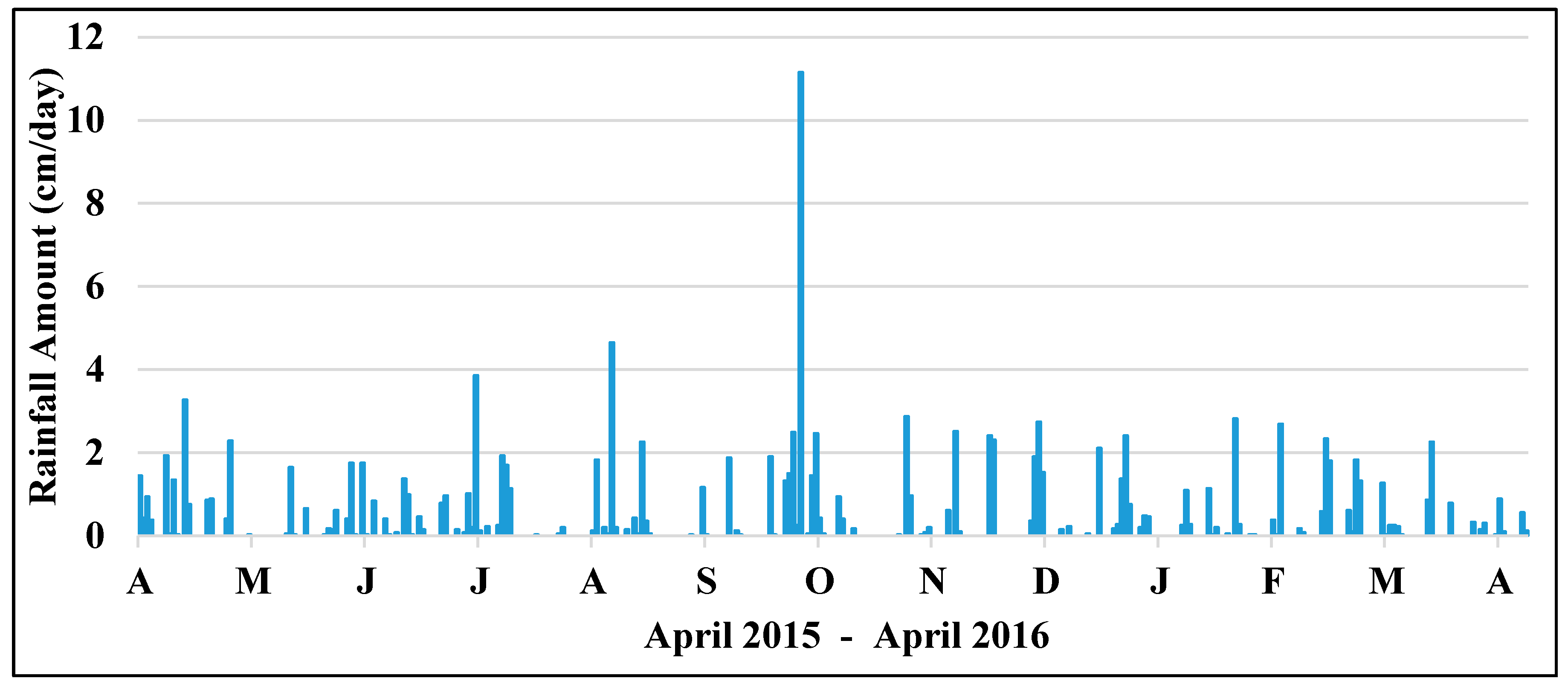
Figure 3.
A comparison of the four skid trail closeout best management practices (BMPs) used in the study.
Figure 3.
A comparison of the four skid trail closeout best management practices (BMPs) used in the study.
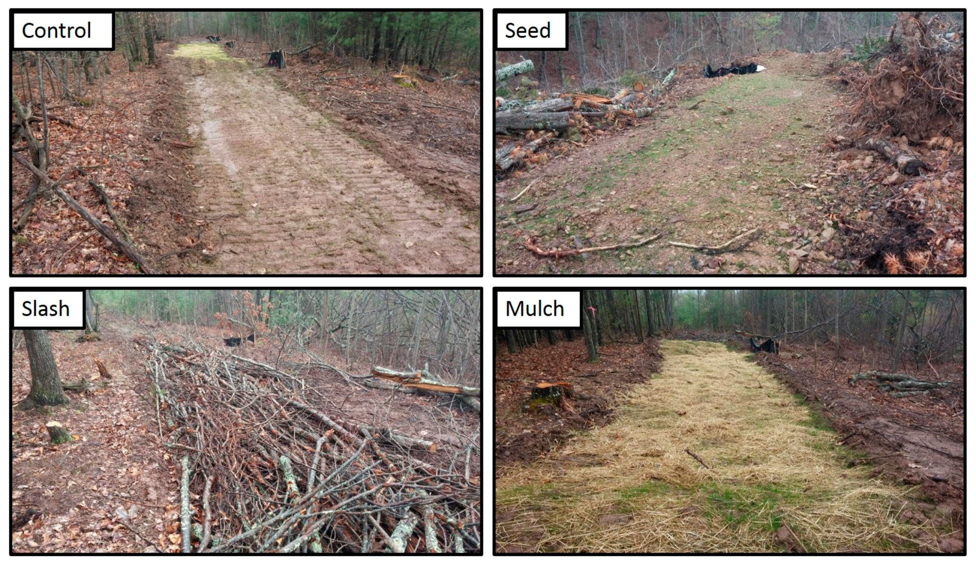
Figure 4.
An example of the silt fence sediment traps used in the study. Sediment pins were driven into trap area on a grid pattern and measured at regular intervals.
Figure 4.
An example of the silt fence sediment traps used in the study. Sediment pins were driven into trap area on a grid pattern and measured at regular intervals.

Figure 5.
(a) Profile of skid trail treatment. Section 1 and Section 2 (lower side of upslope waterbar and skid trail surface) were modeled together; Section 3 (upper side of downslope waterbar) was modeled separately; (b) Photographs of a Mulch treatment from the upslope waterbar looking down toward treatment, downslope waterbar, and sediment trap (first photograph), and from the sediment trap looking upslope to waterbar at top of treatment (second photograph).
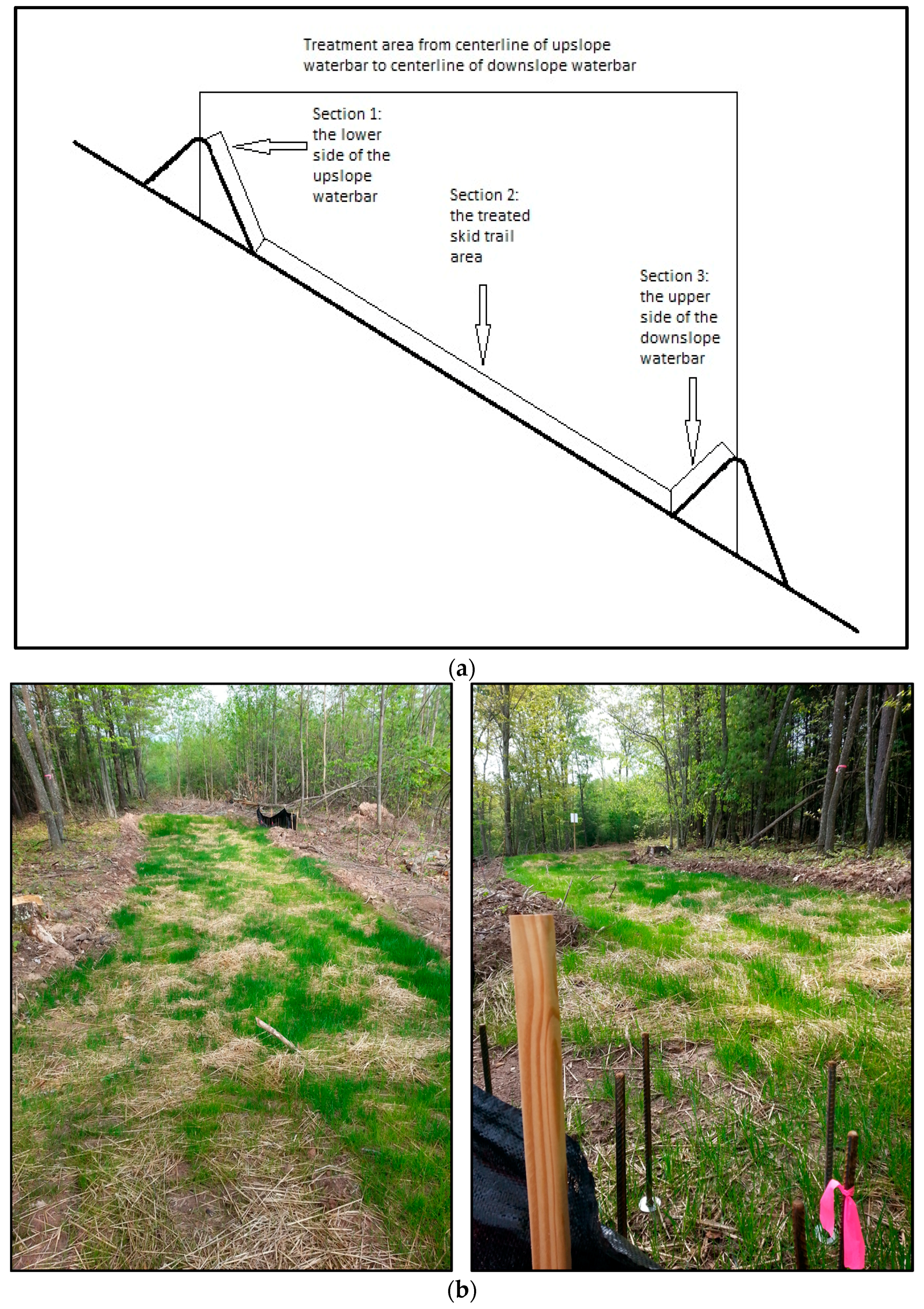
Figure 6.
Linear relationship of RUSLE2 modeled data and actual measured erosion data. Line on graph represents a 1:1 relationship.
Figure 6.
Linear relationship of RUSLE2 modeled data and actual measured erosion data. Line on graph represents a 1:1 relationship.

Figure 7.
Linear relationship of WEPP-Road modeled data and actual measured erosion data. Line on graph represents a 1:1 relationship.
Figure 7.
Linear relationship of WEPP-Road modeled data and actual measured erosion data. Line on graph represents a 1:1 relationship.

Figure 8.
Linear relationship of USLE-Forest modeled data and actual measured erosion data. Line on graph represents a 1:1 relationship.
Figure 8.
Linear relationship of USLE-Forest modeled data and actual measured erosion data. Line on graph represents a 1:1 relationship.
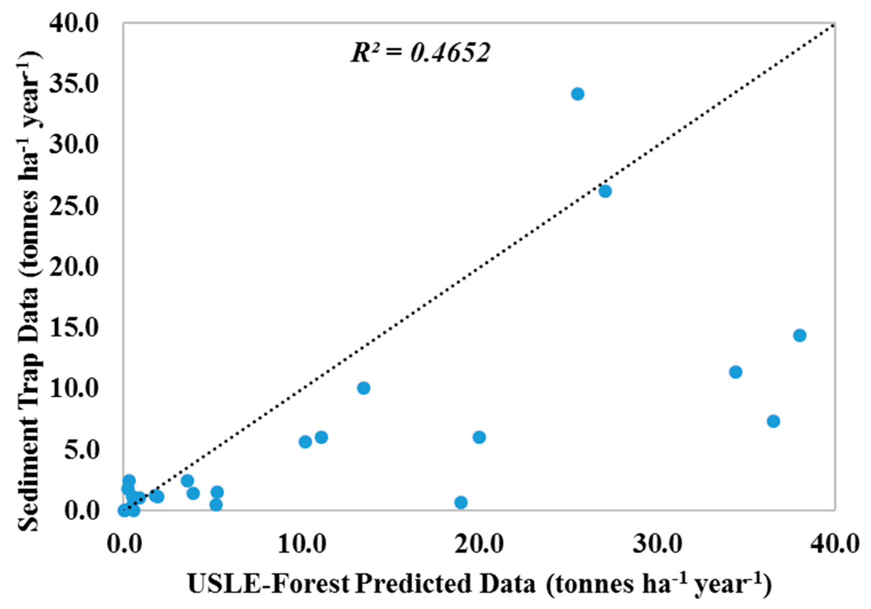
Figure 9.
Linear relationship of WEPP-Road: Modified modeled data and actual erosion data. Line on graph represents a 1:1 relationship.
Figure 9.
Linear relationship of WEPP-Road: Modified modeled data and actual erosion data. Line on graph represents a 1:1 relationship.

Table 1.
Summary statistics for each of the models analyzed. For each treatment, there is an asterisk (*) next to the model prediction that is closest to the measured amount.
Table 1.
Summary statistics for each of the models analyzed. For each treatment, there is an asterisk (*) next to the model prediction that is closest to the measured amount.
| Treatment | Method | Erosion Rate (tonnes ha-1 year−1) | Std Dev a | Std Error Mean b | Lower 95% | Upper 95% |
|---|---|---|---|---|---|---|
| Control | Measured | 15.2 | 12.1 | 5.0 | 2.4 | 27.9 |
| USLE-Forest c | 24.1 | 11.3 | 4.6 | 12.3 | 36.0 | |
| RUSLE2 d | 66.4 | 29.2 | 11.9 | 35.8 | 97.1 | |
| WEPP-Road e: Default | 27.1 | 6.9 | 2.8 | 19.8 | 34.3 | |
| WEPP-Road e: Modified | * 10.8 | 9.5 | 3.9 | 0.8 | 20.7 | |
| Seed | Measured | 5.9 | 5.4 | 2.2 | 0.2 | 11.6 |
| USLE-Forest c | 16.5 | 12.5 | 5.1 | 3.4 | 29.7 | |
| RUSLE2 d | * 6.4 | 3.6 | 1.5 | 2.6 | 10.2 | |
| WEPP-Road e: Default | 12.7 | 6.2 | 2.5 | 6.2 | 19.2 | |
| WEPP-Road e: Modified | 2.8 | 2.3 | 0.9 | 0.4 | 5.2 | |
| Mulch | Measured | 1.1 | 1.0 | 0.4 | 0.1 | 2.1 |
| USLE-Forestc | 0.3 | 0.3 | 0.1 | 0.0 | 0.7 | |
| RUSLE2 d | * 0.6 | 0.4 | 0.2 | 0.2 | 1.1 | |
| WEPP-Road e: Default | 1.6 | 0.7 | 0.3 | 0.9 | 2.4 | |
| WEPP-Road e: Modified | 0.5 | 0.2 | 0.1 | 0.2 | 0.7 | |
| Slash | Measured | 0.8 | 0.6 | 0.2 | 0.2 | 1.4 |
| USLE-Forest c | * 2.3 | 1.9 | 0.8 | 0.3 | 4.3 | |
| RUSLE2 d | 21.8 | 11.0 | 4.5 | 10.3 | 33.3 | |
| WEPP-Road e: Default | 7.3 | 3.6 | 1.5 | 3.5 | 11.0 | |
| WEPP-Road e: Modified | 2.4 | 1.8 | 0.7 | 0.5 | 4.2 |
a Standard Deviation; b Standard Error of the Mean; c Univsersal Soil Loss Equation—Forest; d Revised Universal Soil Loss Equation, v.2; e Water Erosion Prediction Project—Road.
Table 2.
A comparison of predicted erosion rates and their Nash-Sutcliffe Model Efficiency (NSE) values for the whole model and for each treatment type.
Table 2.
A comparison of predicted erosion rates and their Nash-Sutcliffe Model Efficiency (NSE) values for the whole model and for each treatment type.
| Control | Seed | Mulch | Slash | Whole Model NSE a | ||
|---|---|---|---|---|---|---|
| Trapped Sediment | (tonnes ha-1 year-1) | 15.15 | 5.87 | 1.10 | 0.78 | -- |
| USLE-Forest b | (tonnes ha-1 year-1) | 24.14 | 16.54 | 0.33 | 2.30 | -- |
| NSE a | −476.81 | −276.44 | −0.29 | −4.87 | −146.35 | |
| RUSLE2 c | (tonnes ha-1 year-1) | 66.44 | 6.36 | 0.62 | 21.77 | -- |
| NSEa | −5681.25 | −8.90 | 0.23 | −651.77 | −1174.15 | |
| WEPP-Road d: Default | (tonnes ha-1 year-1) | 27.06 | 12.70 | 1.62 | 7.25 | -- |
| NSE a | −442.32 | −94.39 | 0.15 | −60.95 | −115.01 | |
| WEPP-Road d: Modified | (tonnes ha-1 year-1) | 10.75 | 2.05 | 0.45 | 2.37 | -- |
| NSE a | −520.42 | −46.55 | −0.24 | −4.49 | −102.72 |
a Nash-Sutcliffe Model Efficiency; b Univsersal Soil Loss Equation—Forest; c Revised Universal Soil Loss Equation, v.2; d Water Erosion Prediction Project—Road.
Table 3.
Nonparametric analysis comparing each model to the measured data using Wilcoxon method. α = 0.05.
Table 3.
Nonparametric analysis comparing each model to the measured data using Wilcoxon method. α = 0.05.
| Model | Score Mean Difference | Standard Error Difference | p-Value |
|---|---|---|---|
| USLE-Forest a | 4.13 | 4.04 | 0.3074 |
| RUSLE2 b | 9.79 | 4.04 | * 0.0154 |
| WEPP-Road c: Default | 11.45 | 4.04 | * 0.0046 |
| WEPP-Road c: Modified | −1.88 | 4.04 | 0.6427 |
a Univsersal Soil Loss Equation—Forest; b Revised Universal Soil Loss Equation, v.2; c Water Erosion Prediction Project—Road.
© 2017 by the authors. Licensee MDPI, Basel, Switzerland. This article is an open access article distributed under the terms and conditions of the Creative Commons Attribution (CC BY) license (http://creativecommons.org/licenses/by/4.0/).
Share and Cite
MDPI and ACS Style
Vinson, J.A.; Barrett, S.M.; Aust, W.M.; Bolding, M.C. Suitability of Soil Erosion Models for the Evaluation of Bladed Skid Trail BMPs in the Southern Appalachians. Forests 2017, 8, 482. https://doi.org/10.3390/f8120482
AMA Style
Vinson JA, Barrett SM, Aust WM, Bolding MC. Suitability of Soil Erosion Models for the Evaluation of Bladed Skid Trail BMPs in the Southern Appalachians. Forests. 2017; 8(12):482. https://doi.org/10.3390/f8120482
Chicago/Turabian StyleVinson, J. Andrew, Scott M. Barrett, W. Michael Aust, and M. Chad Bolding. 2017. "Suitability of Soil Erosion Models for the Evaluation of Bladed Skid Trail BMPs in the Southern Appalachians" Forests 8, no. 12: 482. https://doi.org/10.3390/f8120482
Note that from the first issue of 2016, this journal uses article numbers instead of page numbers. See further details here.