Vicariance and Oceanic Barriers Drive Contemporary Genetic Structure of Widespread Mangrove Species Sonneratia alba J. Sm in the Indo-West Pacific

 , and add
Show full author list
, and add
Show full author list
Abstract
:1. Introduction
2. Materials and Methods
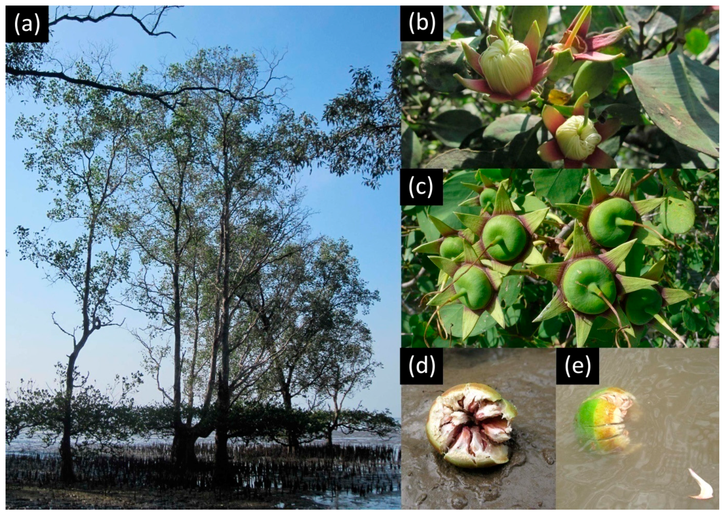
2.1. Study Species
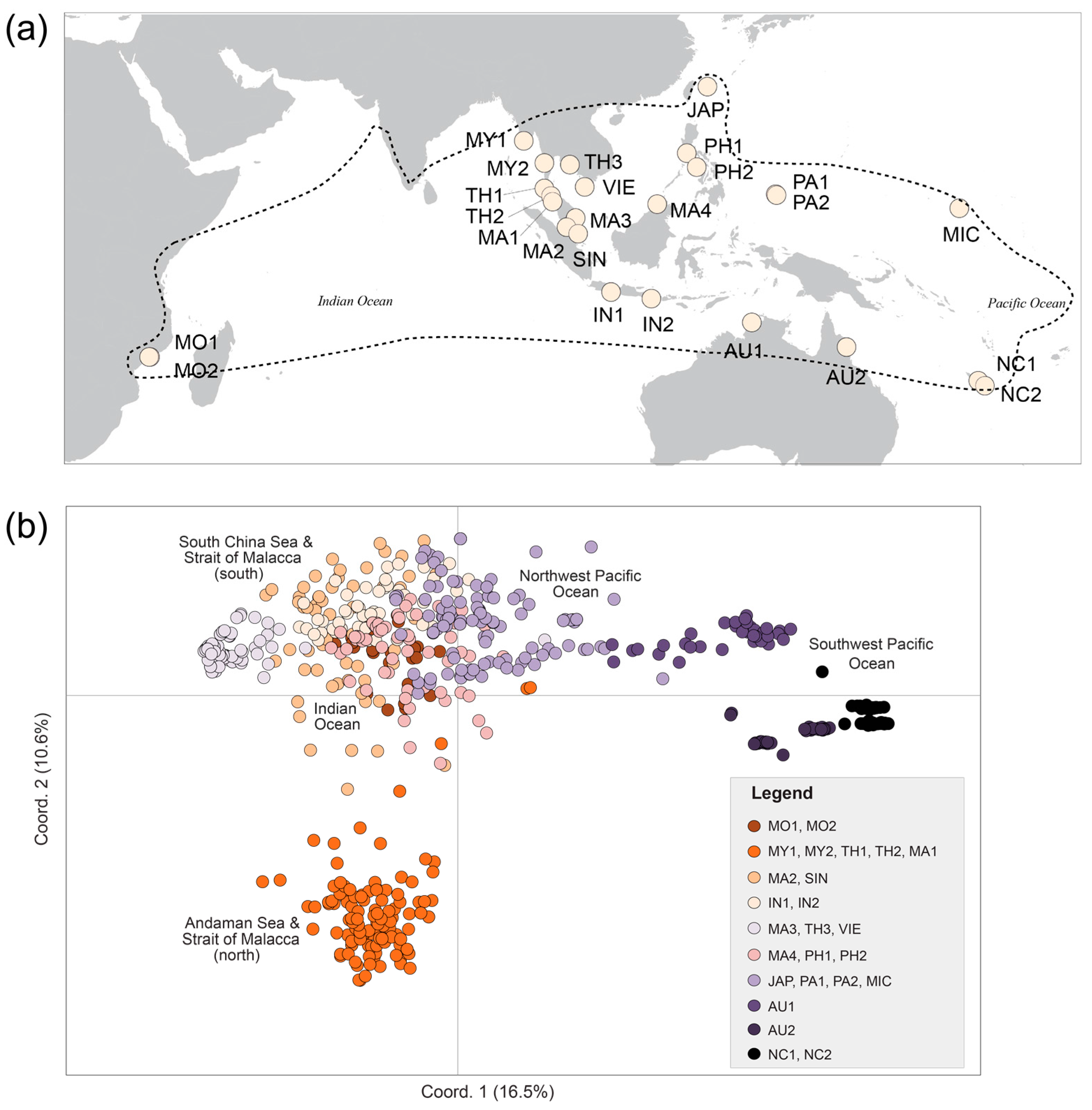
2.2. Plant Material
2.3. DNA Extraction and Genotyping
2.4. Nuclear Microsatellite Data Analysis
2.5. Chloroplast Sequence Data Analysis
3. Results
3.1. Data Quality
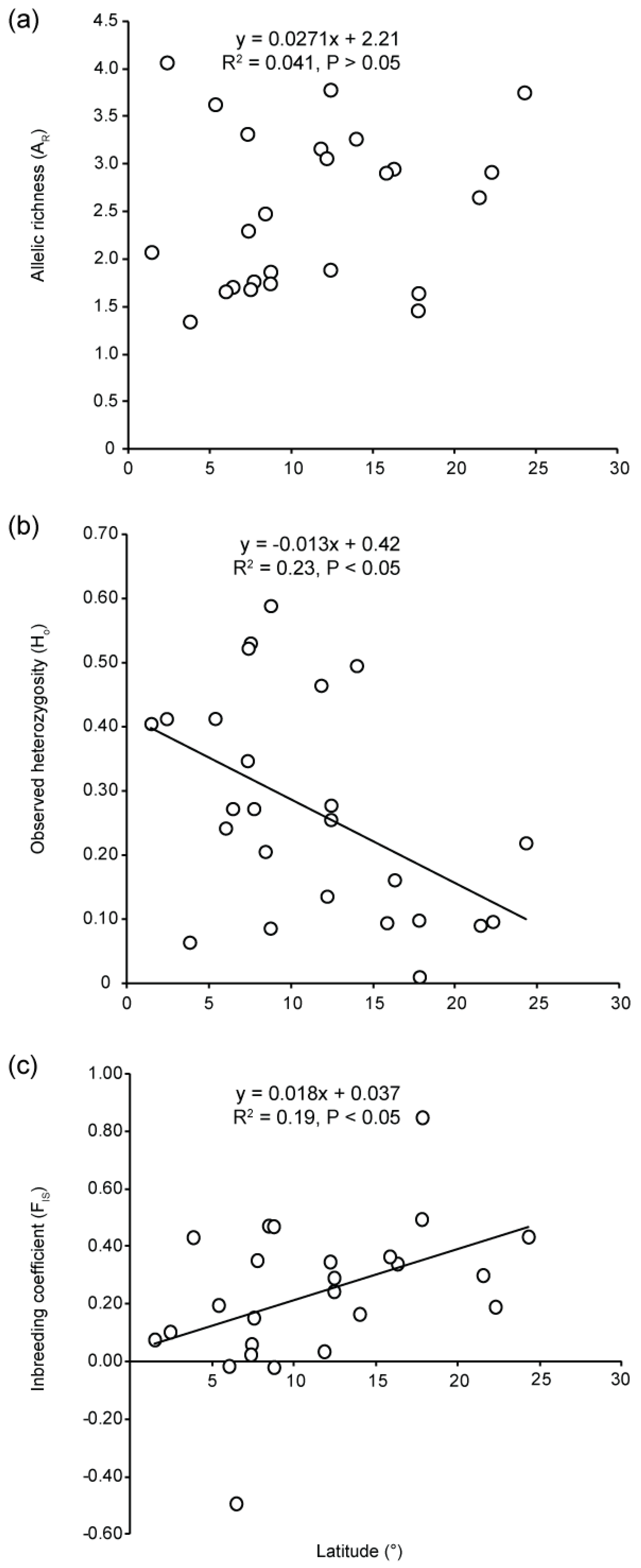
3.2. Genetic Diversity
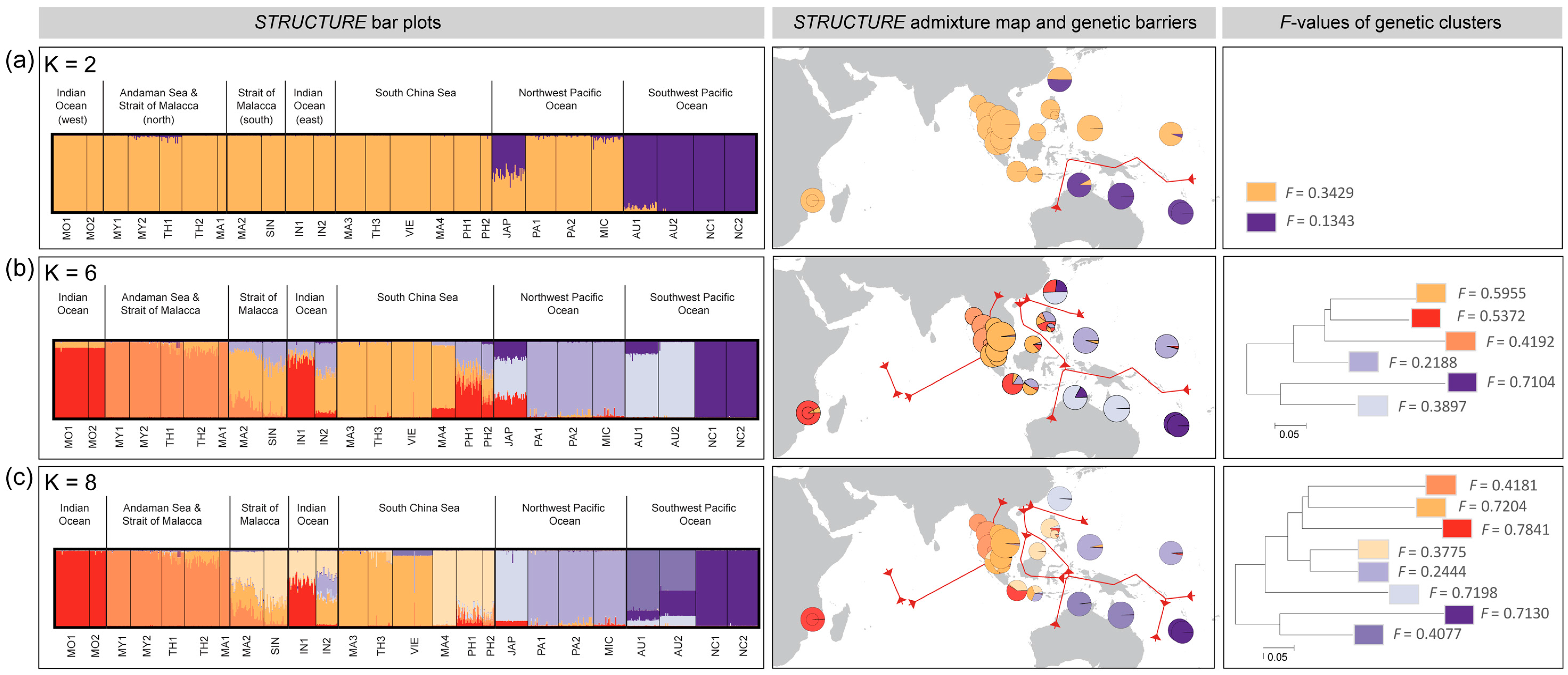
3.3. Population Differentiation and Genetic Structure
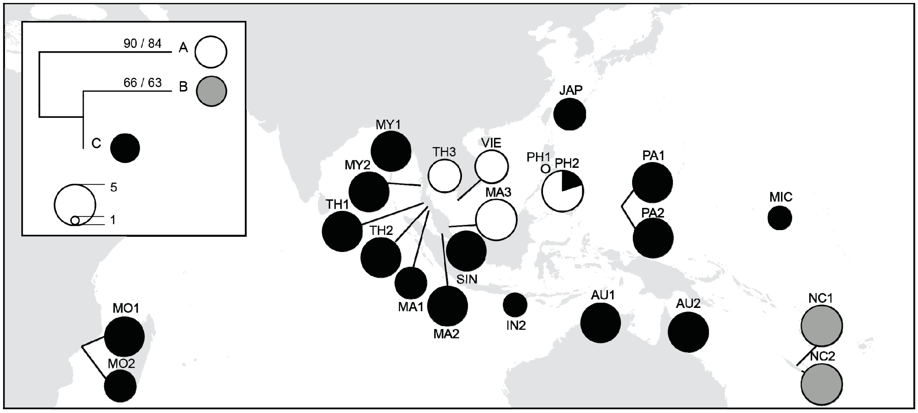
3.4. Chloroplast DNA Variations
4. Discussion
4.1. Majorphylogeographic Break between Indo-Malesia and Australasia
4.2. Strong Influence of Vicariance and Oceanic Barriers on Genetic Structure
4.3. Restricted Gene Flow
4.4. Low Genetic Diversity and High Genetic Drift at Range Edge
5. Conclusions
Supplementary Materials
Acknowledgments
Author Contributions
Conflicts of Interest
References
- Duke, N.; Lo, E.; Sun, M. Global distribution and genetic discontinuities of mangroves—Emerging patterns in the evolution of rhizophora. Trees Struct. Funct. 2002, 16, 65–79. [Google Scholar] [CrossRef]
- Cerón-Souza, I.; Gonzalez, E.G.; Schwarzbach, A.E.; Salas-Leiva, D.E.; Rivera-Ocasio, E.; Toro-Perea, N.; Bermingham, E.; McMillan, W.O. Contrasting demographic history and gene flow patterns of two mangrove species on either side of the central american isthmus. Ecol. Evol. 2015, 5, 3486–3499. [Google Scholar] [CrossRef] [PubMed]
- Takayama, K.; Tamura, M.; Tateishi, Y.; Webb, E.L.; Kajita, T. Strong genetic structure over the american continents and transoceanic dispersal in the mangrove genus rhizophora (rhizophoraceae) revealed by broad-scale nuclear and chloroplast DNA analysis. Am. J. Bot. 2013, 100, 1191–1201. [Google Scholar] [CrossRef] [PubMed]
- Minobe, S.; Fukui, S.; Saiki, R.; Kajita, T.; Changtragoon, S.; Ab Shukor, N.A.; Latiff, A.; Ramesh, B.; Koizumi, O.; Yamazaki, T. Highly differentiated population structure of a mangrove species, Bruguiera gymnorhiza (Rhizophoraceae) revealed by one nuclear gapcp and one chloroplast intergenic spacer TRNF–TRNL. Conserv. Genet. 2010, 11, 301–310. [Google Scholar] [CrossRef]
- Huang, Y.; Tan, F.; Su, G.; Deng, S.; He, H.; Shi, S. Population genetic structure of three tree species in the mangrove genus Ceriops (Rhizophoraceae) from the indo West Pacific. Genetica 2008, 133, 47–56. [Google Scholar] [CrossRef] [PubMed]
- Su, G.-H.; Huang, Y.-L.; Tan, F.-X.; Ni, X.-W.; Tang, T.; Shi, S.-H. Genetic variation in Lumnitzera racemosa, a mangrove species from the indo-west pacific. Aquat. Bot. 2006, 84, 341–346. [Google Scholar] [CrossRef]
- Wee, A.K.; Takayama, K.; Asakawa, T.; Thompson, B.; Sungkaew, S.; Tung, N.X.; Nazre, M.; Soe, K.K.; Tan, H.T.; Watano, Y.; et al. Oceanic currents, not land masses, maintain the genetic structure of the mangrove Rhizophora mucronata Lam. (Rhizophoraceae) in southeast asia. J. Biogeogr. 2014, 41, 954–964. [Google Scholar] [CrossRef]
- Wee, A.K.; Takayama, K.; Chua, J.L.; Asakawa, T.; Meenakshisundaram, S.H.; Adjie, B.; Ardli, E.R.; Sungkaew, S.; Malekal, N.B.; Tung, N.X.; et al. Genetic differentiation and phylogeography of partially sympatric species complex Rhizophora mucronata Lam. and R. stylosa Griff. Using SSR markers. BMC Evol. Biol. 2015, 15, 57. [Google Scholar] [CrossRef] [PubMed]
- Tomlinson, P.B. The Botany of Mangroves; Cambridge University Press: Cambridge, UK, 1986. [Google Scholar]
- Spalding, M.D.; Kainuma, M.; Collins, L. World Atlas of Mangrove; Earthscan: New York, NY, USA, 2010; p. 304. [Google Scholar]
- Yang, Y.; Li, J.; Yang, S.; Li, X.; Fang, L.; Zhong, C.; Duke, N.C.; Zhou, R.; Shi, S. Effects of pleistocene sea-level fluctuations on mangrove population dynamics: A lesson from Sonneratia alba. BMC Evol. Biol. 2017, 17, 22. [Google Scholar] [CrossRef] [PubMed]
- Zhou, R.; Ling, S.; Zhao, W.; Osada, N.; Chen, S.; Zhang, M.; He, Z.; Bao, H.; Zhong, C.; Zhang, B.; et al. Population genetics in nonmodel organisms: II. Natural selection in marginal habitats revealed by deep sequencing on dual platforms. Mol. Biol. Evol. 2011, 28, 2833–2842. [Google Scholar] [CrossRef] [PubMed]
- Onrizal, O.; Mansor, M. Status of coastal forests of the northern sumatra in 2004’s tsunami catastrophe. Biodivers. J. Biol. Divers. 2016, 17, 44–54. [Google Scholar] [CrossRef]
- Ball, M.C.; Pidsley, S.M. Growth responses to salinity in relation to distribution of two mangrove species, Sonneratia alba and S. lanceolata, in Northern Australia. Funct. Ecol. 1995, 9, 77–85. [Google Scholar] [CrossRef]
- Mazda, Y.; Magi, M.; Ikeda, Y.; Kurokawa, T.; Asano, T. Wave reduction in a mangrove forest dominated by sonneratia sp. Wetl. Ecol. Manag. 2006, 14, 365–378. [Google Scholar] [CrossRef]
- Primack, R.B.; Duke, N.C.; Tomlinson, P.B. Floral morphology in relation to pollination ecology in five queensland coastal plants. Austrobaileya 1981, 1, 346–355. [Google Scholar]
- Doyle, J.J.; Doyle, J.L. A rapid DNA isolation procedure for small quantities of fresh leaf tissue. Phytochem. Bull. 1987, 19, 11–15. [Google Scholar]
- Shinmura, Y.; Wee, A.; Takayama, K.; Asakawa, T.; Yllano, O.; Salmo, S.; Ardli, E.; Tung, N.; Malekal, N.; Onrizal, O.; et al. Development and characterization of 15 polymorphic microsatellite loci in Sonneratia alba (Lythraceae) using next-generation sequencing. Conserv. Genet. Resour. 2012, 4, 811–814. [Google Scholar] [CrossRef]
- Hamilton, M. Four primer pairs for the amplification of chloroplast intergenic regions with intraspecific variation. Mol. Ecol. 1999, 8, 521–523. [Google Scholar] [PubMed]
- Jordan, W.C.; Courtney, M.W.; Neigel, J.E. Low levels of intraspecific genetic variation at a rapidly evolving chloroplast DNA locus in north american duckweeds (Lemnaceae). Am. J. Bot. 1996, 430–439. [Google Scholar] [CrossRef]
- Goudet, J. Fstat (Version 2.9.3.): A Program to Estimate and Test Gene Diversities and Fixation Indices. Available online: http://www2.unil.ch/popgen/softwares/fstat.htm (accessed on 5 June 2014).
- Dempster, A.P.; Laird, N.M.; Rubin, D.B. Maximum likelihood from incomplete data via the EM algorithm. J. R. Stat. Soc. B Methodol. 1977, 39, 1–38. [Google Scholar]
- Chapuis, M.-P.; Estoup, A. Microsatellite null alleles and estimation of population differentiation. Mol. Biol. Evol. 2007, 24, 621–631. [Google Scholar] [CrossRef] [PubMed]
- Weir, B.S.; Cockerham, C.C. Estimating f-statistics for the analysis of population structure. Evolution 1984, 38, 1358–1370. [Google Scholar] [PubMed]
- Peakall, R.; Smouse, P. Genalex 6.5: Genetic analysis in excel. Population genetic software for teaching and research—An update. Bioinformatics 2012, 28, 2537–2539. [Google Scholar] [CrossRef] [PubMed]
- Piry, S.; Luikart, G.; Cornuet, J.-M. Bottleneck: A program for detecting recent effective population size reductions from allele data frequencies. J. Heredity 1999, 90, 502–503. [Google Scholar] [CrossRef]
- Meirmans, P.G.; Hedrick, P.W. Assessing population structure: Fst and related measures. Mol. Ecol. Resour. 2011, 11, 5–18. [Google Scholar] [CrossRef] [PubMed]
- Pritchard, J.K.; Stephens, M.; Donnelly, P. Inference of population structure using multilocus genotype data. Genetics 2000, 155, 945–959. [Google Scholar] [PubMed]
- Falush, D.; Stephens, M.; Pritchard, J.K. Inference of population structure using multilocus genotype data: Linked loci and correlated allele frequencies. Genetics 2003, 164, 1567–1587. [Google Scholar] [PubMed]
- Hubisz, M.J.; Falush, D.; Stephens, M.; Pritchard, J.K. Inferring weak population structure with the assistance of sample group information. Mol. Ecol. Resour. 2009, 9, 1322–1332. [Google Scholar] [CrossRef] [PubMed]
- Evanno, G.; Regnaut, S.; Goudet, J. Detecting the number of clusters of individuals using the software Structure: A simulation study. Mol. Ecol. 2005, 14, 2611–2620. [Google Scholar] [CrossRef] [PubMed]
- Earl, D.; vonHoldt, B. Structure harvester: A website and program for visualizing structure output and implementing the Evanno method. Conserv. Genet. Resour. 2012, 4, 359–361. [Google Scholar] [CrossRef]
- Kopelman, N.M.; Mayzel, J.; Jakobsson, M.; Rosenberg, N.A.; Mayrose, I. Clumpak: A program for identifying clustering modes and packaging population structure inferences across K. Mol. Ecol. Resour. 2015, 15, 1179–1191. [Google Scholar] [CrossRef] [PubMed]
- Langella, O. Populations 1.2.28. Population Genetic Software (Individuals or Populations Distances, Phylogenetic Trees); The French National Center for Scientific Research (CNRS): Paris, France, 2002.
- Manni, F.; Guerard, E.; Heyer, E. Geographic patterns of (genetic, morphologic, linguistic) variation: How barriers can be detected by using Monmonier’s algorithm. Hum. Biol. 2004, 76, 173–190. [Google Scholar] [CrossRef] [PubMed]
- Dodd, R.S.; Afzal-Rafii, Z.; Kashani, N.; Budrick, J. Land barriers and open oceans: Effects on gene diversity and population structure in Avicennia germinans L. (avicenniaceae). Mol. Ecol. 2002, 11, 1327–1338. [Google Scholar] [CrossRef] [PubMed]
- Oksanen, J.; Kindt, R.; Legendre, P.; O’Hara, B.; Stevens, M.H.H.; Oksanen, M.J.; Suggests, M. The vegan package. Community Ecol. Package 2007, 10, 631–637. [Google Scholar]
- Kumar, S.; Stecher, G.; Tamura, K. Mega7: Molecular evolutionary genetics analysis version 7.0 for bigger datasets. Mol. Biol. Evol. 2016, 33, 1870–1874. [Google Scholar] [CrossRef] [PubMed]
- Posada, D. Jmodeltest: Phylogenetic model averaging. Mol. Biol. Evol. 2008, 25, 1253–1256. [Google Scholar] [CrossRef] [PubMed]
- Hasegawa, M.; Kishino, H.; Yano, T.-A. Dating of the human-ape splitting by a molecular clock of mitochondrial DNA. J. Mol. Evol. 1985, 22, 160–174. [Google Scholar] [CrossRef] [PubMed]
- Gascuel, O. Bionj: An improved version of the NJ algorithm based on a simple model of sequence data. Mol. Biol. Evol. 1997, 14, 685–695. [Google Scholar] [CrossRef] [PubMed]
- QGIS Desktop v2.18.10. Available online: www.qgis.org (accessed on 17 November 2016).
- DIVA-GIS. Available online: www.diva-gis.org/gdata (accessed on 17 November 2016).
- Lo, E.Y.; Duke, N.C.; Sun, M. Phylogeographic pattern of Rhizophora (Rhizophoraceae) reveals the importance of both vicariance and long-distance oceanic dispersal to modern mangrove distribution. BMC Evol. Biol. 2014, 14, 83. [Google Scholar] [CrossRef] [PubMed] [Green Version]
- Voris, H.K. Maps of Pleistocene sea levels in southeast asia: Shorelines, river systems and time durations. J. Biogeogr. 2000, 27, 1153–1167. [Google Scholar] [CrossRef]
- Saint-Cast, F.; Condie, S.A. Circulation Modelling in Torres Strait; Geoscience Australia: Canberra, Australia, 2006.
- Mirams, A.; Treml, E.; Shields, J.; Liggins, L.; Riginos, C. Vicariance and dispersal across an intermittent barrier: Population genetic structure of marine animals across the Torres strait land bridge. Coral Reefs 2011, 30, 937–949. [Google Scholar] [CrossRef]
- Planes, S.; Fauvelot, C. Isolation by distance and vicariance drive genetic structure of a coral reef fish in the Pacific Ocean. Evolution 2002, 56, 378–399. [Google Scholar] [CrossRef] [PubMed]
- Chiang, T.Y.; Chiang, Y.C.; Chen, Y.J.; Chou, C.H.; Havanond, S.; Hong, T.N.; Huang, S. Phylogeography of Kandelia candel in east Asiatic mangroves based on nucleotide variation of chloroplast and mitochondrial DNAs. Mol. Ecol. 2001, 10, 2697–2710. [Google Scholar] [CrossRef] [PubMed]
- Ngeve, M.N.; Van der Stocken, T.; Menemenlis, D.; Koedam, N.; Triest, L. Contrasting effects of historical sea level rise and contemporary ocean currents on regional gene flow of Rhizophora racemosa in Eastern Atlantic mangroves. PLoS ONE 2016, 11, e0150950. [Google Scholar] [CrossRef] [PubMed]
- Lohman, D.J.; Bruyn, M.; Page, T.; Rintelen, K.; Hall, R.; Ng, P.K.; Shih, H.-T.; Carvalho, G.R.; Rintelen, T. Biogeography of the Indo-Australian Archipelago. Annu. Rev. Ecol. Evol. Syst. 2011, 42, 205–226. [Google Scholar] [CrossRef]
- Barber, P.; Palumbi, S.; Erdmann, M.; Moosa, M. Sharp genetic breaks among populations of Haptosquilla pulchella (Stomatopoda) indicate limits to larval transport: Patterns, causes, and consequences. Mol. Ecol. 2002, 11, 659–674. [Google Scholar] [CrossRef] [PubMed]
- Benzie, J.A. Major genetic differences between crown-of-thorns starfish (Acanthaster planci) populations in the Indian and Pacific Oceans. Evolution 1999, 53, 1782–1795. [Google Scholar] [PubMed]
- Barber, P.H.; Erdmann, M.V.; Palumbi, S.R. Comparative phylogeography of three codistributed Stomatopods: Origins and timing of regional lineage diversification in the Coral Triangle. Evolution 2006, 60, 1825–1839. [Google Scholar] [CrossRef] [PubMed]
- Taylor, M.S.; Hellberg, M.E. Genetic evidence for local retention of pelagic larvae in a Caribbean reef fish. Science 2003, 299, 107–109. [Google Scholar] [CrossRef] [PubMed]
- Di Nitto, D.; Erftemeijer, P.; van Beek, J.; Dahdouh-Guebas, F.; Higazi, L.; Quisthoudt, K.; Jayatissa, L.; Koedam, N. Modelling drivers of mangrove propagule dispersal and restoration of abandoned shrimp farms. Biogeosci. Discuss. 2013, 10, 1267–1312. [Google Scholar] [CrossRef]
- Rabinowitz, D. Dispersal properties of mangrove propagules. Biotropica 1978, 10, 47–57. [Google Scholar] [CrossRef]
- Vargas, P.; Nogales, M.; Jaramillo, P.; Olesen, J.M.; Traveset, A.; Heleno, R. Plant colonization across the galápagos islands: Success of the sea dispersal syndrome. Bot. J. Linn. Soc. 2014, 174, 349–358. [Google Scholar] [CrossRef]
- Gamache, I.; Jaramillo-Correa, J.P.; Payette, S.; Bousquet, J. Diverging patterns of mitochondrial and nuclear DNA diversity in subarctic black spruce: Imprint of a founder effect associated with postglacial colonization. Mol. Ecol. 2003, 12, 891–901. [Google Scholar] [CrossRef] [PubMed]
- Källström, B.; Nyqvist, A.; Åberg, P.; Bodin, M.; André, C. Seed rafting as a dispersal strategy for eelgrass (Zostera marina). Aquat. Bot. 2008, 88, 148–153. [Google Scholar] [CrossRef]
- Tsuda, Y.; Nakao, K.; Ide, Y.; Tsumura, Y. The population demography of Betula maximowicziana, a cool-temperate tree species in Japan, in relation to the last glacial period: Its admixture-like genetic structure is the result of simple population splitting not admixing. Mol. Ecol. 2015, 24, 1403–1418. [Google Scholar] [CrossRef] [PubMed]
- Arnaud-Haond, S.; Teixeira, S.; Massa, S.I.; Billot, C.; Saenger, P.; Coupland, G.; Duarte, C.M.; Serrao, E.A. Genetic structure at range edge: Low diversity and high inbreeding in southeast asian mangrove (Avicennia marina) populations. Mol. Ecol. 2006, 15, 3515–3525. [Google Scholar] [CrossRef] [PubMed]
- De Ryck, D.J.; Koedam, N.; Van der Stocken, T.; van der Ven, R.M.; Adams, J.; Triest, L. Dispersal limitation of the mangrove Avicennia marina at its South African range limit in strong contrast to connectivity in its core East African region. Mar. Ecol. Prog. Ser. 2016, 545, 123–134. [Google Scholar] [CrossRef]
- Islam, M.S.; Lian, C.; Kameyama, N.; Hogetsu, T. Low genetic diversity and limited gene flow in a dominant mangrove tree species (Rhizophora stylosa) at its northern biogeographical limit across the chain of three Sakishima islands of the Japanese archipelago as revealed by chloroplast and nuclear SSR analysis. Plant Syst. Evol. 2014, 300, 1123–1136. [Google Scholar]
- Sexton, J.P.; McIntyre, P.J.; Angert, A.L.; Rice, K.J. Evolution and ecology of species range limits. Annu. Rev. Ecol. Evol. Syst. 2009, 40, 415–436. [Google Scholar] [CrossRef]
- Cordellier, M.; Pfenninger, M. Inferring the past to predict the future: Climate modelling predictions and phylogeography for the freshwater gastropod Radix balthica (Pulmonata, Basommatophora). Mol. Ecol. 2009, 18, 534–544. [Google Scholar] [CrossRef] [PubMed]


| Pop. Code | N | Location | Country | Major Region-Minor Region | Latitude | Longitude |
|---|---|---|---|---|---|---|
| MO1 | 34 | Espinho | Mozambique | WIO | 17°45′38″ S | 37°11′36″ E |
| MO2 | 17 | Zalala Beach | Mozambique | WIO | 17°47′43″ S | 37°04′33″ E |
| MY1 | 25 | Myanmar | Myanmar | EIO-Andaman Sea | 15°48′39″ N | 95°16′09″ E |
| MY2 | 32 | Myanmar | Myanmar | EIO-Andaman Sea | 12°23′53″ N | 98°34′11″ E |
| TH1 | 23 | Phuket | Thailand | EIO-Strait of Malacca | 08°24′28″ N | 98°30′42″ E |
| TH2 | 36 | Kantang | Thailand | EIO-Strait of Malacca | 07°19′13″ N | 99°29′27″ E |
| MA1 | 10 | Langkawi | Malaysia | EIO-Strait of Malacca | 06°25′14″ N | 99°49′19″ E |
| MA2 | 35 | Linggi | Malaysia | EIO-Strait of Malacca | 02°23′34″ N | 101°58′42″ E |
| SIN | 24 | SungeiBuloh | Singapore | EIO-Strait of Malacca | 01°26′54″ N | 103°43′51″ E |
| IN1 | 29 | Cilacap | Indonesia | EIO-East Indian Ocean | 07°42′33″ S | 108°54′00″ E |
| IN2 | 22 | Bali | Indonesia | EIO-Java Sea | 08°44′01″ S | 115°11′48″ E |
| MA3 | 31 | Kuantan | Malaysia | SCS | 03°47′57″ N | 103°19′33″ E |
| TH3 | 25 | Nam Chiao | Thailand | SCS | 12°09′57″ N | 102°28′36″ E |
| VIE | 41 | Ca Mau | Vietnam | SCS | 08°42′51″ N | 104°48′58″ E |
| MA4 | 24 | Sabah | Malaysia | SCS | 05°59′25″ N | 116°05′29″ E |
| PH1 | 27 | Batangas | Philippines | SCS | 13°58′11″ N | 120°37′33″ E |
| PH2 | 12 | Panay | Philippines | SCS | 11°48′09″ N | 122°12′26″ E |
| JAP | 34 | Iriomote | Japan | NPO | 24°16′50″ N | 123°52′58″ E |
| PA1 | 31 | Palau | Palau | NPO | 07°30′13″ N | 134°32′09″ E |
| PA2 | 36 | Palau | Palau | NPO | 07°22′04″ N | 134°34′35″ E |
| MIC | 33 | Kosrae | Micronesia | NPO | 05°21′03″ N | 163°01′12″ E |
| AU1 | 37 | Daintree | Australia | NA | 16°16′45″ S | 145°26′22″ E |
| AU2 | 34 | Ludmila Creek | Australia | NA | 12°24′30″ S | 130°49′57″ E |
| NC1 | 31 | Baie de Tare | New Caledonia | SPO | 22°15′48″ S | 167°00′57″ E |
| NC2 | 32 | Canala | New Caledonia | SPO | 21°30′23″ S | 165°58′12″ E |
| Pop. Code | AR | PA | HO | HE | HS | FIS | Bottleneck |
|---|---|---|---|---|---|---|---|
| MO1 | 1.637 | 0 | 0.099 ± 0.033 | 0.192 ± 0.061 | 0.196 | 0.496 * | No |
| MO2 | 1.338 | 0 | 0.011 ± 0.007 | 0.068 ± 0.038 | 0.072 | 0.850 * | No |
| MY1 | 1.739 | 0 | 0.095 ± 0.042 | 0.146 ± 0.063 | 0.150 | 0.366 * | No |
| MY2 | 2.645 | 2 | 0.256 ± 0.063 | 0.332 ± 0.076 | 0.339 | 0.245 * | No |
| TH1 | 2.902 | 1 | 0.206 ± 0.065 | 0.378 ± 0.085 | 0.390 | 0.473 * | No |
| TH2 | 2.911 | 1 | 0.347 ± 0.087 | 0.351 ± 0.09 | 0.357 | 0.025 | No |
| MA1 | 1.455 | 1 | 0.273 ± 0.129 | 0.178 ± 0.070 | 0.183 | −0.492 | Yes |
| MA2 | 3.055 | 1 | 0.413 ± 0.059 | 0.454 ± 0.055 | 0.461 | 0.104 | No |
| SIN | 2.944 | 1 | 0.405 ± 0.059 | 0.429 ± 0.060 | 0.439 | 0.077 | No |
| IN1 | 2.474 | 2 | 0.273 ± 0.038 | 0.412 ± 0.056 | 0.422 | 0.353 * | No |
| IN2 | 3.747 | 2 | 0.589 ± 0.066 | 0.565 ± 0.065 | 0.578 | −0.019 | No |
| MA3 | 1.655 | 0 | 0.065 ± 0.040 | 0.111 ± 0.061 | 0.114 | 0.433 * | No |
| TH3 | 1.883 | 2 | 0.136 ± 0.053 | 0.203 ± 0.071 | 0.209 | 0.348 * | No |
| VIE | 1.760 | 2 | 0.086 ± 0.038 | 0.160 ± 0.054 | 0.164 | 0.471 * | No |
| MA4 | 1.702 | 2 | 0.242 ± 0.082 | 0.234 ± 0.077 | 0.239 | −0.015 | No |
| PH1 | 3.775 | 1 | 0.496 ± 0.048 | 0.581 ± 0.056 | 0.594 | 0.166 * | No |
| PH2 | 3.311 | 0 | 0.465 ± 0.057 | 0.461 ± 0.055 | 0.482 | 0.036 | No |
| JPN | 2.069 | 0 | 0.219 ± 0.042 | 0.380 ± 0.071 | 0.388 | 0.435 * | No |
| PA1 | 4.062 | 2 | 0.531 ± 0.036 | 0.615 ± 0.042 | 0.626 | 0.153 * | No |
| PA2 | 3.622 | 2 | 0.523 ± 0.077 | 0.549 ± 0.052 | 0.557 | 0.061 | No |
| MIC | 3.157 | 2 | 0.413 ± 0.063 | 0.506 ± 0.066 | 0.515 | 0.197 * | Yes |
| AU1 | 3.26 | 5 | 0.278 ± 0.076 | 0.385 ± 0.102 | 0.393 | 0.292 * | No |
| AU2 | 2.293 | 8 | 0.162 ± 0.068 | 0.241 ± 0.096 | 0.245 | 0.341 * | No |
| NC1 | 1.678 | 0 | 0.091 ± 0.068 | 0.127 ± 0.087 | 0.130 | 0.301 * | Yes |
| NC2 | 1.862 | 1 | 0.097 ± 0.063 | 0.117 ± 0.077 | 0.120 | 0.191 | No |
| Mean | 2.517 | 1.5 | 0.271 ± 0.016 | 0.327 ± 0.017 | 0.335 |
| MO1 | MO2 | MY1 | MY2 | TH1 | TH2 | MA1 | MA2 | SIN | IN1 | IN2 | MA3 | TH3 | VIE | MA4 | PH1 | PH2 | JPN | PA1 | PA2 | MIC | AU1 | AU2 | NC1 | NC2 | |
|---|---|---|---|---|---|---|---|---|---|---|---|---|---|---|---|---|---|---|---|---|---|---|---|---|---|
| MO1 | *** | *** | *** | *** | *** | *** | *** | *** | *** | *** | *** | *** | *** | *** | *** | *** | *** | *** | *** | *** | *** | *** | *** | *** | |
| MO2 | 0.319 | *** | *** | *** | *** | ** | *** | *** | *** | *** | *** | *** | *** | *** | *** | *** | *** | *** | *** | *** | *** | *** | *** | *** | |
| MY1 | 0.705 | 0.819 | *** | *** | *** | *** | *** | *** | *** | *** | *** | *** | *** | *** | *** | *** | *** | *** | *** | *** | *** | *** | *** | *** | |
| MY2 | 0.634 | 0.684 | 0.377 | *** | *** | *** | *** | *** | *** | *** | *** | *** | *** | *** | *** | *** | *** | *** | *** | *** | *** | *** | *** | *** | |
| TH1 | 0.629 | 0.664 | 0.372 | 0.206 | *** | *** | *** | *** | *** | *** | *** | *** | *** | *** | *** | *** | *** | *** | *** | *** | *** | *** | *** | *** | |
| TH2 | 0.608 | 0.645 | 0.327 | 0.142 | 0.076 | *** | *** | *** | *** | *** | *** | *** | *** | *** | *** | *** | *** | *** | *** | *** | *** | *** | *** | *** | |
| MA1 | 0.768 | 0.863 | 0.646 | 0.426 | 0.352 | 0.344 | *** | *** | *** | *** | *** | *** | *** | *** | *** | ** | *** | *** | *** | *** | *** | *** | *** | *** | |
| MA2 | 0.593 | 0.612 | 0.564 | 0.428 | 0.400 | 0.391 | 0.473 | *** | *** | *** | *** | *** | *** | *** | *** | *** | *** | *** | *** | *** | *** | *** | *** | *** | |
| SIN | 0.621 | 0.650 | 0.643 | 0.514 | 0.478 | 0.484 | 0.536 | 0.085 | *** | *** | *** | *** | *** | *** | *** | *** | *** | *** | *** | *** | *** | *** | *** | *** | |
| IN1 | 0.347 | 0.427 | 0.601 | 0.541 | 0.510 | 0.509 | 0.598 | 0.424 | 0.400 | *** | *** | *** | *** | *** | *** | *** | *** | *** | *** | *** | *** | *** | *** | *** | |
| IN2 | 0.499 | 0.514 | 0.555 | 0.438 | 0.392 | 0.409 | 0.514 | 0.250 | 0.256 | 0.264 | *** | *** | *** | *** | *** | *** | *** | *** | *** | *** | *** | *** | *** | *** | |
| MA3 | 0.759 | 0.849 | 0.794 | 0.644 | 0.636 | 0.582 | 0.813 | 0.456 | 0.510 | 0.610 | 0.407 | *** | *** | *** | *** | *** | *** | *** | *** | *** | *** | *** | *** | *** | |
| TH3 | 0.679 | 0.769 | 0.702 | 0.569 | 0.552 | 0.514 | 0.732 | 0.350 | 0.400 | 0.523 | 0.332 | 0.262 | *** | *** | *** | *** | *** | *** | *** | *** | *** | *** | *** | *** | |
| VIE | 0.698 | 0.772 | 0.760 | 0.627 | 0.632 | 0.573 | 0.768 | 0.407 | 0.493 | 0.568 | 0.407 | 0.514 | 0.463 | *** | *** | *** | *** | *** | *** | *** | *** | *** | *** | *** | |
| MA4 | 0.722 | 0.769 | 0.746 | 0.631 | 0.612 | 0.596 | 0.736 | 0.449 | 0.476 | 0.576 | 0.473 | 0.719 | 0.627 | 0.667 | *** | *** | *** | *** | *** | *** | *** | *** | *** | *** | |
| PH1 | 0.444 | 0.484 | 0.494 | 0.393 | 0.367 | 0.384 | 0.481 | 0.307 | 0.274 | 0.239 | 0.228 | 0.518 | 0.422 | 0.513 | 0.414 | *** | *** | *** | *** | *** | *** | *** | *** | *** | |
| PH2 | 0.611 | 0.685 | 0.619 | 0.513 | 0.450 | 0.463 | 0.571 | 0.406 | 0.379 | 0.349 | 0.286 | 0.659 | 0.537 | 0.665 | 0.569 | 0.238 | *** | *** | *** | *** | *** | *** | *** | *** | |
| JPN | 0.597 | 0.641 | 0.660 | 0.560 | 0.517 | 0.548 | 0.664 | 0.489 | 0.513 | 0.496 | 0.410 | 0.639 | 0.588 | 0.644 | 0.626 | 0.372 | 0.501 | *** | *** | *** | *** | *** | *** | *** | |
| PA1 | 0.496 | 0.499 | 0.536 | 0.450 | 0.412 | 0.437 | 0.461 | 0.296 | 0.285 | 0.336 | 0.239 | 0.544 | 0.455 | 0.527 | 0.482 | 0.292 | 0.331 | 0.446 | *** | *** | *** | *** | *** | *** | |
| PA2 | 0.524 | 0.507 | 0.580 | 0.485 | 0.442 | 0.470 | 0.521 | 0.343 | 0.326 | 0.425 | 0.271 | 0.545 | 0.465 | 0.533 | 0.483 | 0.311 | 0.366 | 0.488 | 0.174 | *** | *** | *** | *** | *** | |
| MIC | 0.559 | 0.572 | 0.588 | 0.515 | 0.464 | 0.484 | 0.539 | 0.361 | 0.330 | 0.364 | 0.317 | 0.588 | 0.501 | 0.564 | 0.509 | 0.325 | 0.361 | 0.524 | 0.228 | 0.309 | *** | *** | *** | *** | |
| AU1 | 0.666 | 0.688 | 0.707 | 0.619 | 0.587 | 0.607 | 0.665 | 0.551 | 0.562 | 0.562 | 0.479 | 0.704 | 0.659 | 0.714 | 0.663 | 0.489 | 0.517 | 0.541 | 0.457 | 0.468 | 0.506 | *** | *** | *** | |
| AU2 | 0.751 | 0.794 | 0.760 | 0.667 | 0.654 | 0.661 | 0.745 | 0.631 | 0.663 | 0.660 | 0.599 | 0.811 | 0.766 | 0.793 | 0.751 | 0.583 | 0.669 | 0.633 | 0.556 | 0.571 | 0.606 | 0.555 | *** | *** | |
| NC1 | 0.820 | 0.880 | 0.845 | 0.745 | 0.722 | 0.709 | 0.832 | 0.650 | 0.702 | 0.716 | 0.646 | 0.863 | 0.819 | 0.836 | 0.804 | 0.617 | 0.725 | 0.697 | 0.604 | 0.601 | 0.646 | 0.658 | 0.729 | *** | |
| NC2 | 0.824 | 0.888 | 0.851 | 0.748 | 0.716 | 0.711 | 0.841 | 0.675 | 0.725 | 0.724 | 0.662 | 0.871 | 0.825 | 0.841 | 0.810 | 0.637 | 0.734 | 0.716 | 0.612 | 0.603 | 0.655 | 0.661 | 0.738 | 0.504 |
| AR | HO | HS | FIS | FST | |
|---|---|---|---|---|---|
| Core | 2.727 | 0.334 | 0.394 | 0.152 | 0.449 |
| Peripheral | 2.291 | 0.191 | 0.272 | 0.298 | 0.66 |
| p-value | 0.193 | 0.031 | 0.070 | 0.031 | 0.010 |
© 2017 by the authors. Licensee MDPI, Basel, Switzerland. This article is an open access article distributed under the terms and conditions of the Creative Commons Attribution (CC BY) license (http://creativecommons.org/licenses/by/4.0/).
Share and Cite
Wee, A.K.S.; Teo, J.X.H.; Chua, J.L.; Takayama, K.; Asakawa, T.; Meenakshisundaram, S.H.; Onrizal; Adjie, B.; Ardli, E.R.; Sungkaew, S.; et al. Vicariance and Oceanic Barriers Drive Contemporary Genetic Structure of Widespread Mangrove Species Sonneratia alba J. Sm in the Indo-West Pacific. Forests 2017, 8, 483. https://doi.org/10.3390/f8120483
Wee AKS, Teo JXH, Chua JL, Takayama K, Asakawa T, Meenakshisundaram SH, Onrizal, Adjie B, Ardli ER, Sungkaew S, et al. Vicariance and Oceanic Barriers Drive Contemporary Genetic Structure of Widespread Mangrove Species Sonneratia alba J. Sm in the Indo-West Pacific. Forests. 2017; 8(12):483. https://doi.org/10.3390/f8120483
Chicago/Turabian StyleWee, Alison K. S., Jessica Xian Hui Teo, Jasher L. Chua, Koji Takayama, Takeshi Asakawa, Sankararamasubramanian H. Meenakshisundaram, Onrizal, Bayu Adjie, Erwin Riyanto Ardli, Sarawood Sungkaew, and et al. 2017. "Vicariance and Oceanic Barriers Drive Contemporary Genetic Structure of Widespread Mangrove Species Sonneratia alba J. Sm in the Indo-West Pacific" Forests 8, no. 12: 483. https://doi.org/10.3390/f8120483