Mapping Net Stocked Plantation Area for Small-Scale Forests in New Zealand Using Integrated RapidEye and LiDAR Sensors


New Zealand School of Forestry, University of Canterbury, Christchurch 8140, New Zealand
*
Author to whom correspondence should be addressed.
Forests 2017, 8(12), 487; https://doi.org/10.3390/f8120487
Submission received: 4 October 2017
/
Revised: 30 November 2017
/
Accepted: 2 December 2017
/
Published: 7 December 2017
(This article belongs to the Section Forest Inventory, Modeling and Remote Sensing)
Abstract
:In New Zealand, approximately 70% of plantation forests are large-scale (over 1000 ha) with accurate resource description. In contrast, the remaining 30% of plantation forests are small-scale (less than 1000 ha). It is forecasted that these small-scale forests will supply nearly 40% of the national wood production in the next decade. However, in-depth description of these forests, especially those under 100 ha, is very limited. This research evaluates the use of remote sensing datasets to map and estimate the net stocked plantation area for small-scale forests. We compared a factorial combination of two classification approaches (Nearest Neighbour (NN), Classification and Regression Tree (CART)) and two remote sensing datasets (RapidEye, RapidEye plus LiDAR) for their ability to accurately classify planted forest area. CART with a combination of RapidEye and LiDAR metrics outperformed the other three combinations producing the highest accuracy for mapping forest plantations (user’s accuracy = 90% and producer’s accuracy = 88%). This method was further examined by comparing the mapped plantations with manually digitised plantations based on aerial photography. The mapping approach overestimated the plantation area by 3%. It was also found that forest patches exceeding 10 ha achieved higher conformance with the digitised areas. Overall, the mapping approach in this research provided a proof of concept for deriving forest area and mapping boundaries using remote sensing data, and is especially relevant for small-scale forests where limited information is currently available.
1. Introduction
Forestry is a significant industry in New Zealand, being the third largest export earner and contributing approximately $5 billion annually to New Zealand’s economy [1]. New Zealand’s plantation forests, which are dominated by radiata pine (Pinus radiata D. Don), cover approximately 1.70 million hectares as 1 April 2016 [2]. The New Zealand National Exotic Forest Description (NEFD) [2] indicates that approximately 70% of the plantations have an area over 1000 ha and are owned by large-scale owners, who are mainly corporate forest companies. These forests undergo regular monitoring and assessment by professional foresters. The area descriptions of large-scale forest owners are captured from the NEFD annual survey. The information from large-scale owners, especially those with more than 10,000 ha of forests, is considered the most reliable source of NEFD data [2].
On the other hand, the remaining 30% are small-scale plantation forests owned by individual investors, farmers or local governments, who are less likely to have regular area assessment. The forest description of smaller-scale forests is less reliable due to inconsistent area definition and management practices. The data provided by small-scale forest owners is likely to be more variable in terms of reliability as (1) some of the areas reported may well be gross areas rather than net stocked areas; (2) data potentially contain higher non-sampling errors due to reporting inaccuracies and responses based on owners’ estimates and (3) errors raised in transferring non-electronic data into the database [2]. In addition, the NEFD survey only directly surveys 232,000 ha of the 520,000 ha of small-scale forests in New Zealand; most of the remaining area is imputed from annual nursery surveys off the number of seedlings sold [2]. The approach was considered a reasonable and efficient way of estimating, but also less accurate than alternative methods [3]. However, since 2006 new plantings have not been added to the NEFD due to the low levels of new seedlings planted [2]. The limitations of this process are that it does not provide direct measurement of the plantation area, nor describe where the plantations are located.
Overall, the lack of reliability of forest description for small-scale forests has led to insufficient understanding of the wood supply from these forests. These small-scale forests, which were mostly planted in the 1990s, will play an important role in providing wood supply in the next few decades. By 2020, the small-scale forests will have the capacity to provide around 15 million m3 of radiata pine logs per annum, which will be over 40% of the total radiata pine supply [4]. Therefore, it is critical to understand the location and area of these small-scale forests in order to effectively plan marketing, harvesting, logistics and transport capacity that are required for additional wood supply.
A remote sensing solution for small-scale forest description is necessary because conducting a comprehensive survey and field assessment of these patchy forests is impractical due to the substantial time and cost associated with it. The existing spatial description of plantation resources include the Land Cover Database (LCDB) and Land Use Carbon Analysis System (LUCAS) [2]. However, the plantation areas for small-scale forests reported from these sources are gross area, including areas that are not intended for timber production [2], and therefore are an overestimate of the net stocked area. The satellite imagery used to develop the LCDB were SPOT and Landsat [5], which are medium resolution (10–30 m) that potentially overlook small patches of forests and erroneously include gaps in forest area estimates.
Remote sensing has played an important role in forest classification and delineation. Aerial photography has traditionally been the most commonly used approach to determine forest area through manual interpretation despite being potentially subjective and time consuming [6]. Optical sensors such as satellite imagery can also be used in forest classification and delineation, by automatically assigning forest cover types and estimating forest variables with algorithms based on the spectral, textural and auxiliary data in the images [7]. This produces a more objective classification and delineation, which reduces time and associated costs [8,9]. LiDAR as an active sensor adds additional structural information for forest classification and delineation through direct estimation of forest canopy area and height [10,11].
Combining LiDAR with optical sensors has been used in a number of studies and more accurate forest classification and delineation results have been achieved relative to using optical sensors alone [7,12]. Nordkvist, et al. [9] combined LiDAR-derived height metrics and SPOT 5-derived spectral information for vegetation classification, and achieved 16.1% improvement in classification accuracy compared to using SPOT only. Sasaki, et al. [13] improved the overall land cover classification accuracy marginally by 2.5% by using high resolution spectral images and LiDAR-derived metrics including height, ratio [14], pulse and intensity parameters. Furthermore, Bork and Su [8] found that the fusion of LiDAR and multispectral imagery increased classification accuracy by 15–20%. Xu et al. [12] reviewed a number of forest cover classification studies and concluded that using both LiDAR sensor and optical sensors produced up to 20% improvement in classification results compared with using a single sensor.
Object-based image analysis (OBIA) is an image analysis approach that groups and classifies similar pixels (i.e., image objects) rather than individual pixels [15]. Pixel-based image classification tends to be sensitive to spectral variations, hence it is likely to result in a high level of misclassification and reduce the accuracy of classification [16]. OBIA segmentation processes create image objects that are similar to real land cover features in size and shape [17]. The approach allows use of multiple image elements, parameters and scales such as texture, shape and context, as opposed to pixel-based classification that solely relies on the pixel value. Overall, OBIA has been proven to produce more accurate classification results compared to pixel-based approaches using medium to high resolution imagery, producing improvements in classification accuracy ranging from 9–23% [18,19,20].
Two commonly used supervised OBIA classification approaches include Nearest Neighbour (NN) and Classification and Regression Tree (CART). NN classification is a non-parametric classifier, and there is no Gaussian distribution for the input data [21]. The classification algorithm computes the statistical distance iteratively from image objects to be classified to the nearest training sample points and assigns them into that class [22]. NN has been applied in delineating forest polygons with OBIA analysis [22], classifying forested land covers [23], delineating forested and non-forested areas [24] and describing vegetation species composition and structure [25].
CART is also a non-parametric statistical technique that allows selection of the most appropriate explanatory variables through tree form learning, which can be used in data mining [26]. The algorithm allows the classes from representative training samples to be split in an optimal manner. The purpose is to create a model that predicts the land cover of a target object based on attributes attached to training samples. A tree can be “learned” by splitting the source set into subsets based on an attribute value test. This process is repeated on each derived subset in a recursive manner called recursive partitioning. The subsequent subsets are separated further until no further division is possible or the tree reaches a defined maximum depth [26,27]. CART has been used in a number of studies for land cover classification [28], delineating forest boundaries [22] and extracting forest variables [17].
This research aims to evaluate the performance of forest classification and delineation using RapidEye multispectral imagery alone and combined with LiDAR data. RapidEye imagery is a 5-m multispectral sensor containing five spectral bands including blue, green, red, red edge and near-inferred [29]. The aim is to develop an automated approach to detect and provide accurate estimation of the stocked areas for small-scale forests using an OBIA approach. The key objective is to compare the net stocked plantation areas derived by different combinations of remote sensing datasets and mapping approaches with the plantation areas manually digitised from high-resolution aerial photography in order to determine which approach provides the best potential for accurate automated plantation mapping. Specifically, this study will address the following research questions: (1) Which combination of the remote sensing dataset and mapping approach produces the highest classification accuracy? (2) How different is the mapped plantation area compared with the manually digitised plantation area and (3) Is the performance of the classification approach affected by plantation patch size?
2. Materials and Methods
2.1. Study Area
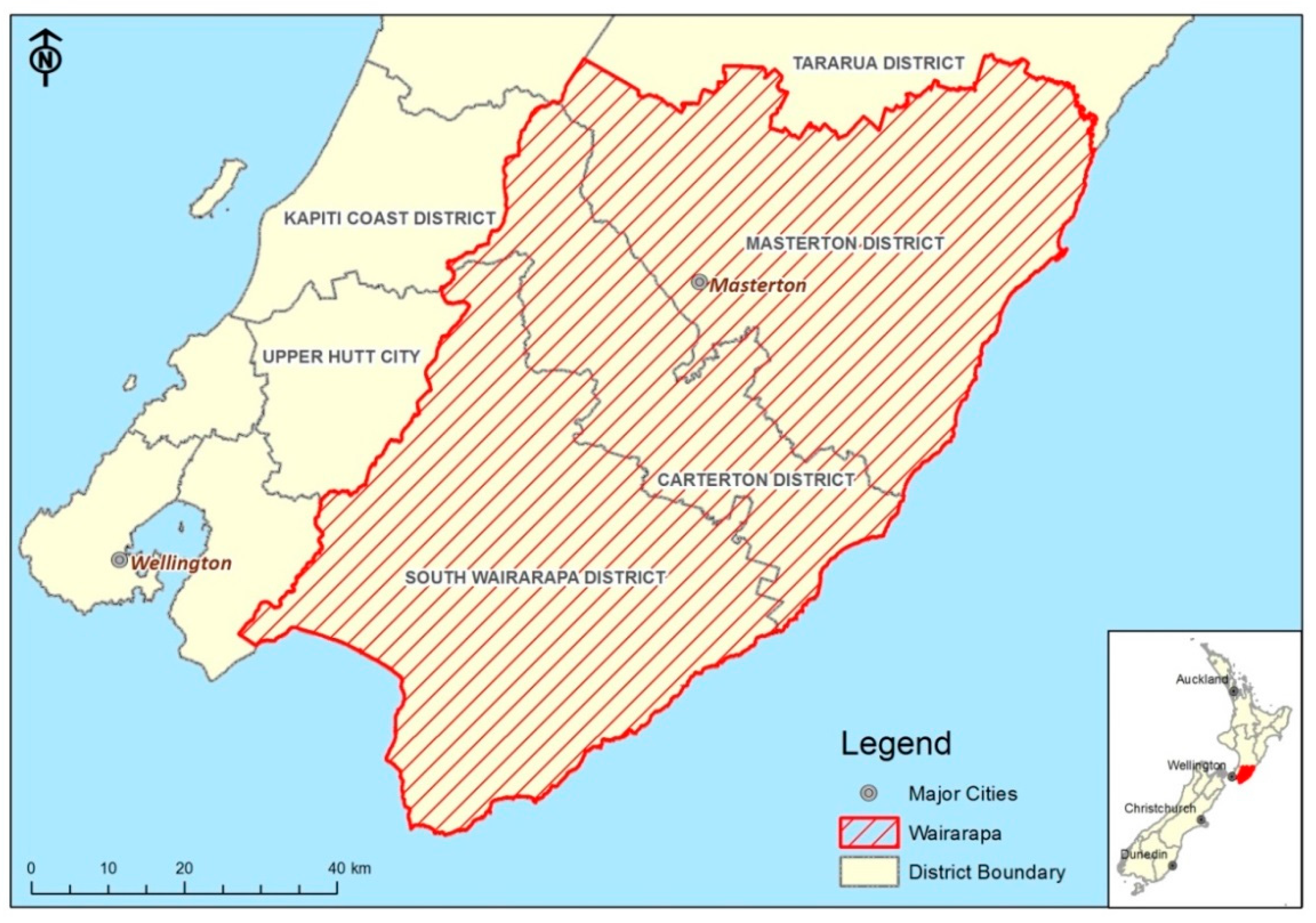
The study area is New Zealand’s Wairarapa region (593,803 ha) (Figure 1). The region mainly contains three types of landscape: the western mountains, the central lowlands and the hilly eastern uplands. The climate is warm and dry, with annual rainfall ranging from 800 to 1200 millimetres and maximum temperatures of 20–28 °C in summer and 10–15 °C in winter [30].
The region consists of three districts: Masterton, Carterton and South Wairarapa. The NEFD indicates there are approximately 51,237 ha of forest plantations in the Wairarapa Region [2], which primarily consist of radiata pine (98%). Other minor planted species include Douglas-fir, cypress and eucalyptus [2]. Approximately 50% of the plantations are owned by small-scale forest owners. This region was selected due to its large area of small-scale plantations and the availability of recent LiDAR coverage.
2.2. Data Preparation
Three sets of remote sensing data: 0.3 m orthorectified aerial photography, airborne LiDAR and Rapid Eye. The Wellington Regional Council (WRC) acquired orthorectified aerial photography between 10 December 2012 and 30 January 2013. In total, 764 aerial photos covered the Wairarapa region. The delivered aerial photographs were used as the basis for manual interpretation of plantation as well as the ground truth dataset, against which classified datasets would be compared.
WRC and Landcare Research provided wall-to-wall LiDAR coverage over the Wairarapa Region. Airborne LiDAR survey data were collected by Aerial Surveys Ltd. (Auckland, New Zealand) from 4 January to 23 December 2013. The flight specifications are listed in Table 1. Landcare Research, as the agent for the WRC, delivered geo-referenced but unclassified raw LiDAR points, in LAS format, in 1 km × 1 km tiles. The planned point density was 1.3 points m−2, the actual point density delivered was much higher due to high swath overlap. The delivered point density differs for each sub-region, but averaged 3.76 points m−2.
LiDAR points from all returns were classified as ground and non-ground points, and a 1 m digital elevation model (DEM), digital surface model (DSM) and canopy height model (CHM) which was calculated by subtracting DEM from DSM, were generated using FUSION (Pacific Northwest Research Station, USDA).
The RapidEye scenes were delivered with radiometric, sensor and geometric corrections applied to the data. A total of 21 cloud-free images were acquired between 13 November 2013 and 20 February 2014. Atmospheric corrections and topographic corrections were applied to all scenes using ATCOR for ERDAS Imagine 2014 (Geosystems GmbH, Germering, Germany). ATCOR was developed by Richter and Schläpfer [31] utilising MODTRAN atmospheric simulation code [32,33]. The algorithm is reported to perform well for a wide range of sensors, terrains and land covers [34,35,36].
The DEM layers used for topographic correction are the National 15 m DEM developed by New Zealand School of Surveying [37]. The DEM was resampled to 5 m to match the 5 m resolution RapidEye imagery. In spite of resampling to 5 m resolution, the topographic correction did not correct any micro relief finer than the original 15 m-resolution. The atmospherically and topographically corrected RapidEye images were represented as surface spectral reflectance. The coordinate system used for all input data was New Zealand Transverse Mercator 2000 (NZTM2000).
2.3. Sample Area Selection
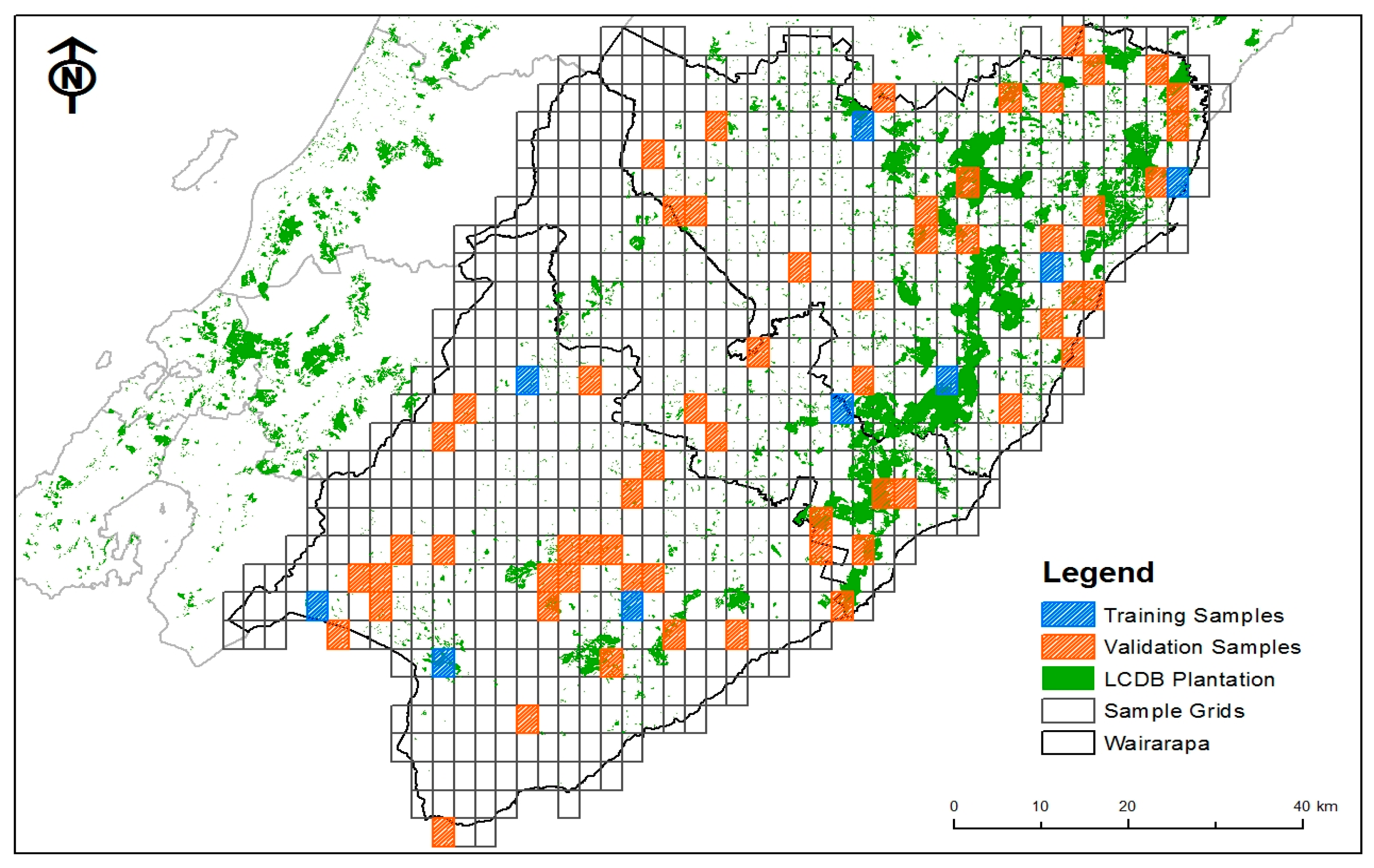
Due to the extensive study area, a stratified random sampling approach was applied to select representative sample areas for developing the mapping approach. The orthophoto survey grids (3.6 km × 2.4 km) were used as sampling grids; in total there were 764 grids covering the Wairarapa region, each being 864 ha (Figure 2).
The New Zealand LCDB is a digital map layer representing the land cover of New Zealand. The plantation areas from the most recent version (LCDB v4.1) were mapped by New Zealand Landcare Research based on 2012 satellite imagery and were overlaid on sampling grids to allow calculation of total plantation area within each grid. Individual grids were then classified into three forest area classes based on total plantation area within each grid:
- Forest Class 1: <10 ha
- Forest Class 2: 10–100 ha
- Forest Class 3: >100 ha
The binomial proportion power calculator developed based on Rosner [38] suggested a minimum of 32 grids be selected as a representative sample of the study area. In total, 69 sample grids were selected to represent the Wairarapa region for plantation derivation. These included nine grids (three randomly selected from each stratified forest area class), which served as the training grids for developing an OBIA forest mapping workflow, and 60 grids (20 randomly selected from each stratified forest area class), which served as the validation grids. The total area of all 69 sample grids was 59,616 ha, which accounted for approximately 10% of the whole Wairarapa area.
2.4. Forest Mapping
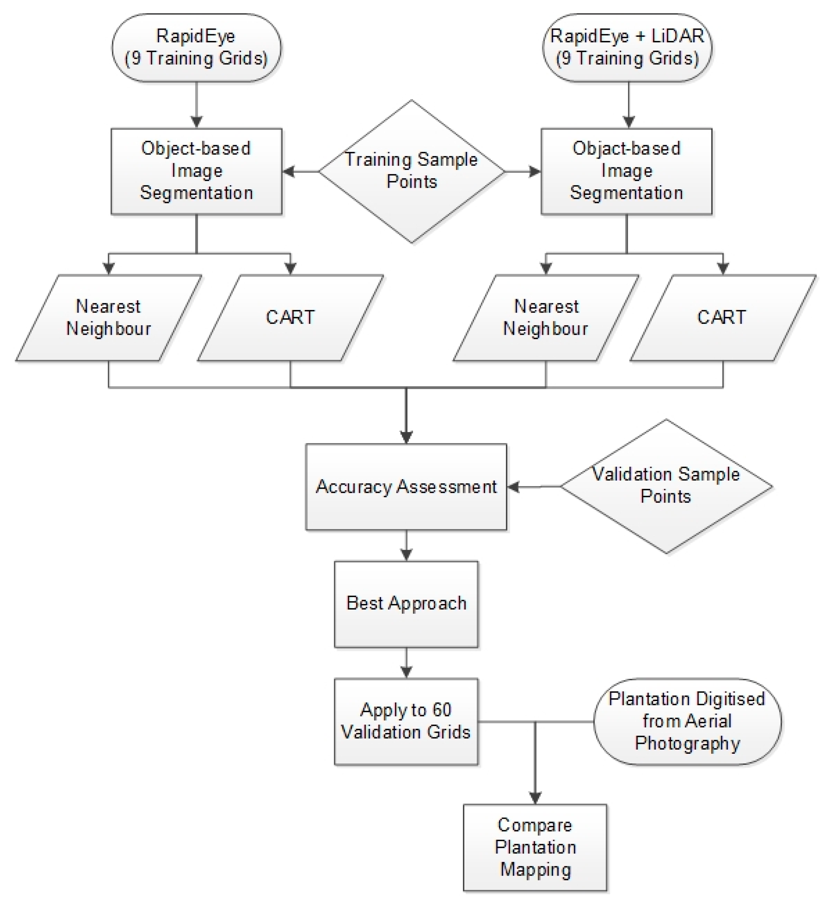
The aim was to develop an automated mapping process for delineating forest plantations using object based image analysis. The segmentation and classification steps for the OBIA are described in detail below; however, a brief overview of the mapping process is described here. The first step was to perform a land cover classification on the nine test grids using only RapidEye imagery and then a fusion of RapidEye and LiDAR-derived grids. Nearest Neighbour (NN) and Classification and Regression Tree (CART) were undertaken on each test grid. Therefore, each test grid was subjected to four classifications as follows:
- NN to RapidEye only (NN-RE)
- NN to RapidEye and LiDAR (NN-RE+LiDAR)
- CART to RapidEye only (CART-RE)
- CART to RapidEye and LiDAR (CART-RE+LiDAR)
The classification accuracies from different sensor and algorithm combinations across the nine training grids were compared with manually digitised plantation areas to determine the approach with the highest accuracy. This approach was selected and applied to the 60 validation grids. The plantation areas in all 69 grids (9 test grids and 60 validation grids) were mapped using the approach with the highest accuracy and were compared with manual digitisation of plantation area from aerial photography. Figure 3 shows an overview of the plantation mapping process.
2.4.1. Segmentation
eCognition Developer 8.8 (Trimble Germany GmbH, München, Germany) was used for the OBIA classification. An important prerequisite for OBIA classification is quality image segmentation. Multi-resolution segmentation was applied to extract meaningful objects by taking account of the scale, shape and context of objects [27]. An estimation of scale parameter (ESP) tool was used to inform the selection of the optimal scale parameter for multi-resolution segmentation. It was implemented as a customised rule set in eCognition that runs multiple segmentations with a defined fixed increment for the scale parameter, and calculates the local variance (LV, the mean standard deviation for all objects) and the rate of change (ROC) to assess the change of LV from one scale level to another [39,40].
ROC = (LV − (LV − 1))/(LV − 1) × 100,
Sample grids with low forest cover (i.e., small and patchy forests) generally required a finer scale factor, whereas grids that contained large and continuous forest cover did not require as fine of scale parameter. Based on both EPS results and visual observation, scale parameters ranging from 100 to 140 were chosen for grids depending on their forest cover class (Table 2).
2.4.2. Classification
Although the key purpose was to map forest plantation area, it is important to include other representative land cover classes in classification so that sources of error can be identified. Six land cover classes were used in this study (Table 3).
NN and CART were evaluated for their utility in land cover classification. For both classification approaches, there were 87 spatial predictors used for RapidEye classification and 99 features used to classify RapidEye combined with LiDAR; these features include built-in features which include the mean, standard deviation, skewness, brightness and texture [41] and geometry related features as well as customised features. Customised spatial predictors refer to band ratios or vegetation indices calculated from RapidEye spectral bands, to provide additional and more standardised spectral description of images. In total, 17 customised predictors were derived based on research from Machala and Zejdova [23] and Rana, et al. [42] (shown in Table 4). All LiDAR-derived grids were re-sampled to 5 m resolution to be consistent with RapidEye imagery. Since LiDAR-derived CHM, DSM, DEM, slope, as well as the standard deviation and skewness of these grids have proven to be useful in differentiating vegetation types [43]; they were also included as the spatial predictors for the NN and CART classification.
Both NN and CART classification algorithms were built into eCognition. For both approaches, sample points that are representative of each land cover class were manually selected in ArcGIS (ESRI, Redlands, CA, USA) based on high resolution aerial photography, and were then used as the training sample points for supervised OBIA classification. A total of 702 sample points representing the six land cover classes were selected for the nine training grids.
Prior to the NN classification, all input features were evaluated using Feature Space Optimisation in eCognition to calculate the best combination of features in the feature space [44]. The Feature Space Optimisation tool calculates the separation Euclidian distance between all samples of all classes with all possible combinations of input features, and finds the feature combination that produces the largest separation distance (which is the largest average minimum distance) between samples of different land cover classes. The combination of features that produces the largest separation distance was selected to use for classification. Feature Space Optimisation was applied to all nine training grids to define the optimal features to be used in the NN classification.
The CART process in eCognition involves defining CART parameters (maximum tree depth, minimum sample per node and cross validation folds) and applying these to the training samples. Different parameter values were tested, but in the end all three parameters were given a value of 10 based on visual assessment of classification. Additionally, the same settings were used in a similar forest classification study [28]. The selection of the spatial predictors was not required for CART classification as the decision tree automatically selected the useful predictors.
2.4.3. Aerial Photo Interpretation
The stocked plantation areas were manually digitised in ArcGIS. Plantation assessment from 0.3 m orthophotos was used as the ground truthing data since aerial photography has higher resolution than other sensors used in this study. In general, the stocked plantation forests showed distinct characteristics on orthophotos, so they were easily differentiated from surrounding land cover classes. Occasionally, image stretching was applied to enhance orthophotos to allow clearer interpretation.
The mapping rules adopted for the manual digitisation process in this study were as follows:
- Maximum mapping scale: 1:1000
- All features were digitised at the maximum scale of 1:1000; some smaller features were digitised at 1:500
- Minimum mapping unit: 0.1 ha
- All isolated forest blocks over 0.1 ha were digitised. Any gaps within forests over 0.05 ha were digitised
- Forest areas less than 15 m wide were excluded, i.e., some narrow shelterbelts were not mapped as forest
- The minimum distance between forest patches was 50 m, if the distance between two mapped forest patches was less than 50 m, they were mapped as one patch. Otherwise, they needed to be digitised as separate forest patches
2.4.4. Initial Accuracy Assessment
Quantitative assessment of classification results was obtained through a confusion matrix, which compares the classification results against corresponding ground truthing data or known reference points [45]. A stratified random sample of points was used for accuracy assessment. The number of points required was calculated based on multinomial probability theory [46,47]. According to this theory, a minimum of 636 points were required for accuracy assessment. The area proportion of each aggregated land cover class from the LCDB was used as a basis to assign the number of points to each land cover class. In total, 1200 points were randomly distributed amongst all land cover classes. A trained aerial photography interpreter was provided with the points and asked to determine the true land cover class for each point. These reference points were then compared with the classified results to establish the confusion matrix. Based on the confusion matrix, the overall accuracy, producer’s accuracy and user’s accuracy were calculated for each land cover class.
The overall accuracy is calculated as the proportion of the number of corrected classified points over the total number of points. The producer’s accuracy (corresponding to the omission error) is the number of correctly classified points of each land cover class divided by the total number of reference points in each corresponding land cover class, which indicates the probability of a reference point being correctly classified. On the other hand, the user’s accuracy (corresponding to commission error) is the number of correctly classified points of each land cover class divided by the total number of points that were classified in that land cover class, it is indicative of the probability that a classified point actually represents that class on ground [45].
Following the automated classification, some post-classification refinements were implemented in a decision tree built manually to correct any obvious misclassification from automated classification. The customised feature Red Edge (RE) Ratio was useful in separating natural and planted forests; and REGNDVI, which is a vegetation index incorporating Red Edge and Green band, was found to be very useful in differentiating vegetation and non-vegetation classes. The description of the refinements is provided in the supplementary material.
2.4.5. Overall Classification Accuracy Assessment
The classification approach was validated using a larger subset of 60 validation grids. The accuracy assessment involved the same approach used for the nine training grids which was establishing a confusion matrix that compared the mapped land cover class with the reference land cover class. A new set of 1200 validation points covering the larger extent was generated and used in classification accuracy assessment.
2.4.6. Assessing the Accuracy of Automatically Classified Plantation Patches
The purpose of the analysis is to evaluate how well the mapping approach delineated forest plantation boundaries. The total plantation area mapped by the mapping approach was compared with the manual interpretation grid by grid for all nine training and 60 validation grids. Additionally, the mapped plantation area for all 69 grids was compared to the latest LCDB plantation area. The comparison only included areas with standing trees so that any harvested areas and areas waiting to be replanted were not included.
To better understand the effect of forest patch size on mapping success, mapped and digitised forest patches were compared. Where a single mapped forest patch corresponded to a single digitised forest patch, it is straight forward to compare the areas. However, where a single mapped forest patch corresponded to two or more digitised patches, or vice-versa, a different approach was required. In such cases, the combined area of the two or more smaller patches was compared to the area of the corresponding single larger patch. For two or more forest patches to be considered as a single patch, they all would have to have some overlap with the single larger polygon or be separated by no more than 50 m. In total, 889 polygons were manually digitised and 584 sets of valid patch-to-patch comparisons were established. This excluded area that did not follow the mapping standards (such as area less than minimum mapping unit of 0.1 ha or shelterbelts that are less than 15 m in width), harvested areas and new plantings. A paired t-test was used to determine whether the mapped and digitised plantation patch areas were statistically different.
3. Results and Discussion
3.1. Initial Land Cover Classification
The classification accuracies for each land cover class achieved by the four combinations of classification approaches are shown in Table 5. The overall classification accuracy was the lowest (60%) when using NN-RE only approach; whereas the classification accuracy was the highest (75%) using CART-RE+LiDAR approach. Using only RapidEye imagery produced overall classification of 60% and 67% for NN and CART respectively. Incorporating LiDAR data has improved the classification accuracy slightly by 3% and 8% respectively for NN and CART. Overall, CART outperformed the NN algorithm in overall classification and most of the individual land cover classifications. However, there was no obvious difference observed in the classification accuracy for bare ground when using different classification approaches, and NN appeared to perform slightly better in classifying the water class. In general, when only RapidEye imagery was used, CART improved the overall classification accuracy by 7%. When incorporating LiDAR data, there was a 12% improvement relative to NN. The superiority of CART was also observed by Mallinis, et al. [22] who found that CART improved classification accuracy by over 20% compared to NN approach in classifying natural forest in Northern Greece.
The improvement of sensor fusion shown here is consistent with what other studies have found although the amount of improvement in this study appears lower compared to Bork and Su [8] and Nordkvist, et al. [9], who saw a 15–20% improvement when combining LiDAR surfaces with optical sensors. Using only RapidEye enables the capture of plantations reasonably well; giving a minimum producer’s accuracy of 80% and a minimum user’s accuracy of 83% both achieved by NN-RE only. There was a small improvement in the producer’s accuracy when incorporating LiDAR features; reaching 82% accuracy with a NN approach and 88% with a CART approach. Using both RapidEye and LiDAR benefited the classification of natural forest and shrubland the most compared to using RapidEye alone. Table 5 indicates that the producer’s accuracy of natural forest has increased by 13% using a NN approach; and the producer’s accuracy of shrubland and scrub has increased by 31% using a CART approach. Both the overall and plantation classification accuracy were highest using the CART approach with both RapidEye and LiDAR data as inputs. Therefore, using CART with both RapidEye and LiDAR data as inputs was chosen as the optimal mapping approach.
Post-classification refinements, detailed in [48] and the supplementary material, were applied to the CART with both the RapidEye and LiDAR approach. The final overall accuracy for all land cover classes increased by 10%, from 75 to 85% (Table 6). The producer’s and user’s accuracy of plantation forests was 89% and 92% respectively. At 85%, the overall classification accuracy is not very high, but is comparable with some recent forest classification studies. Haywood and Stone [49] developed an automated approach that applied aerial photos and LiDAR CHM to delineate Eucalyptus forest boundaries and achieved 65% overall accuracy. Pham, et al. [50] used Quickbird and LiDAR to classify forest species in a New Zealand urban environment and achieved an overall accuracy of 85%. Another OBIA classification by Dupuy, et al. [51] used SPOT 5 and LiDAR surfaces to classify tropical vegetation type and gained 92% overall accuracy.
Despite general improvements in classification, errors for some classes, especially bare ground, still remain. Almost half of the bare ground was misclassified into grassland and in many cases grassland was misclassified as bare ground. The omission errors for planted forests mainly came from natural forests and some from grassland. It was understandable that planted forests tended to have similar spectral signature and height to natural forests, yet the misclassification to grassland raised concerns. Apart from planted forest, natural forests and shrubland also appeared to be misclassified as grassland. In order to further examine these errors, all classification errors were manually reviewed to identify whether the errors were due to the classification approach or another reason.
It was noticed that some of the remaining misclassifications were due to changes that occurred over time; this is a consequence of the RapidEye images being collected approximately one year later than the reference aerial photos. For example, in Figure 4, the aerial photo shows planted forest, but the RapidEye image shows the same area as bare ground which has been harvested. Another factor that affected the classification accuracy was the resolution of RapidEye imagery, which is coarser than aerial photography used for ground truthing. The difference in pixel size could affect the classification accuracy (see example in Figure 5). The classification errors caused by temporal change and resolution difference were quantified after reviewing all classification errors. In total, there were 178 classification errors within all 1200 reference points. It was found that 22 errors, which accounted for 12% of all errors, were due to temporal difference between RapidEye and aerial photographs; and 65 errors, which accounted for 37% of all errors, were due to differences in resolution between RapidEye and aerial photos. If those errors were excluded, the overall classification accuracy would reach 91%. This highlights the importance of obtaining remote sensing data and truthing information at the same time to reduce the errors caused by temporal difference. The difference in the data resolution in this study remains as a limitation of using remote sensing for classification.
3.2. Land Cover Classification of All Validation Grids
Having refined the classification approach to achieve an acceptable accuracy assessment for the nine training grids, the approach was then applied to all 60 validation grids. The overall classification accuracy for the 60 validation grids was 89% (Table 7). Based on producer’s accuracy, grassland, natural forest and water were more accurately classified than bare ground, planted forest and shrubland. This indicates that bare ground, planted forests and shrubland tend to be misclassified into other land cover classes. Based on user’s accuracy, other classes were more likely to be misclassified into bare ground, natural forests and shrubland. The producer’s accuracy for plantation was 79% and user’s accuracy for plantation was 94%, which means that the classification approach tends to under-classify planted forests. The omission error for planted forests was 21% and most of these were contributed by natural forest and shrubland. Similarly, commission occurred when natural forests or shrubland were misclassified as plantations. The commission error for planted forests was much lower at 6%, which suggests the classification approach does not tend to misclassify other classes as planted forests.
The overall accuracy (89%) achieved for all validation grids was also within the range of other studies, but did not reach the accuracies achieved by Hellesen and Matikainen [28] and Sasaki, et al. [13] who produced classification accuracies over 95%. It is worth noting that almost all comparable classification studies were applied on a single study area with limited spatial coverage, ranging from 100 ha to 1500 ha [13,23,28,52]. This study area contains 69 sample grids that are geographically separated from each other, with a total area of 59,616 ha. The largest study area reviewed was by Bork and Su [8], who classified vegetation classes in a rangeland covering 2400 ha and obtained an overall accuracy of 83.9%. Designing a mapping approach that works for a larger study area can be more challenging as more variations need to be taken account, such as topographic variation, spectral variation from satellite imagery and land cover variation.
Since plantations are being actively managed, many misclassifications of plantation are caused by temporal changes such as harvesting and new plantings. By reviewing all 135 classification errors it was found that 33 errors (accounting for 24% of all errors) were caused by temporal change of land cover classes. By excluding the sample points where changes occurred, the producer’s accuracy of plantation increased to 89%, but the user’s accuracy remained unchanged, and the overall accuracy increased by 2% (Table 7). Because the classification approach did not appear to differentiate new plantings and grassland, it tended to misclassify new plantings to grassland or to shrubland if the new plantings were taller. Likewise, the misclassification of bare ground to grassland was also mainly caused by temporal differences in an actively managed agricultural environment. If there was no temporal difference in the image source used, the classification would have been improved especially for dynamic land cover classes such as bare ground and planted forest.
3.3. Plantation Area Comparison
All plantations mapped from nine training grids and 60 validation grids were compared with manually digitised plantations from aerial photography. This was done to gain a better understanding of the limits of automatically mapping forest plantations. Overall, the area of plantation digitised from aerial photography was 485 ha greater than the area mapped using CART approach with RapidEye and LiDAR data (Table 8). In other words, the mapping approach underestimated plantation area by 7.8%. This discrepancy is partly due to resolution, whereby aerial photography has a much finer resolution (0.3 m) than RapidEye and LiDAR (5 m). The finer spatial resolution of the aerial photography allowed detection of additional features such as new plantings during manual digitisation. Such features are less likely to be detected by automated classification of coarser resolution RapidEye. It is possible to derive young plantation areas using finer resolution imagery, as a study by Zhou, et al. [53] using 0.5 m resolution Worldview imagery successfully mapped the growth density of young plantations that were less than two years old.
If we excluded all the new plantings detected during manual digitisation of aerial photography, the mapping approach overestimated the plantation area by 168 ha, which was 3% of the total area digitised. This is understandable as RapidEye and LiDAR have coarser resolution and are more likely to misclassify small forest patches, gaps or roads within forests. The Mean Absolute Error (MAE) and Root-Mean-Square-Error (RMSE) were much lower when new plantings were excluded (Table 8).
3.4. Comparison to LCDB
The latest LCDB indicates that the planted forest area (Class “Exotic Forest” in LCDB) for the nine training grids and validation grids was 6941.6 ha, which is 11% more than the digitised plantation area including new plantings, and 24% more than the digitised plantation area excluding new plantings. This suggests that the current LCDB plantation tends to overestimate the plantation area. Since LCDB is a well-developed mapping system led by Landcare Research with decades of peer-reviewed research [54], this overestimation could be largely due to the use of a coarser sensor SPOT 5, which is 10 m resolution as opposed to 5-m RapidEye. The imagery used for developing LCDB was last acquired in 2012, which is one year older than the aerial photography, and two years older than RapidEye imagery. The temporal difference between LCDB and this study is difficult to assess due to lack of satellite imagery for developing LCDB.
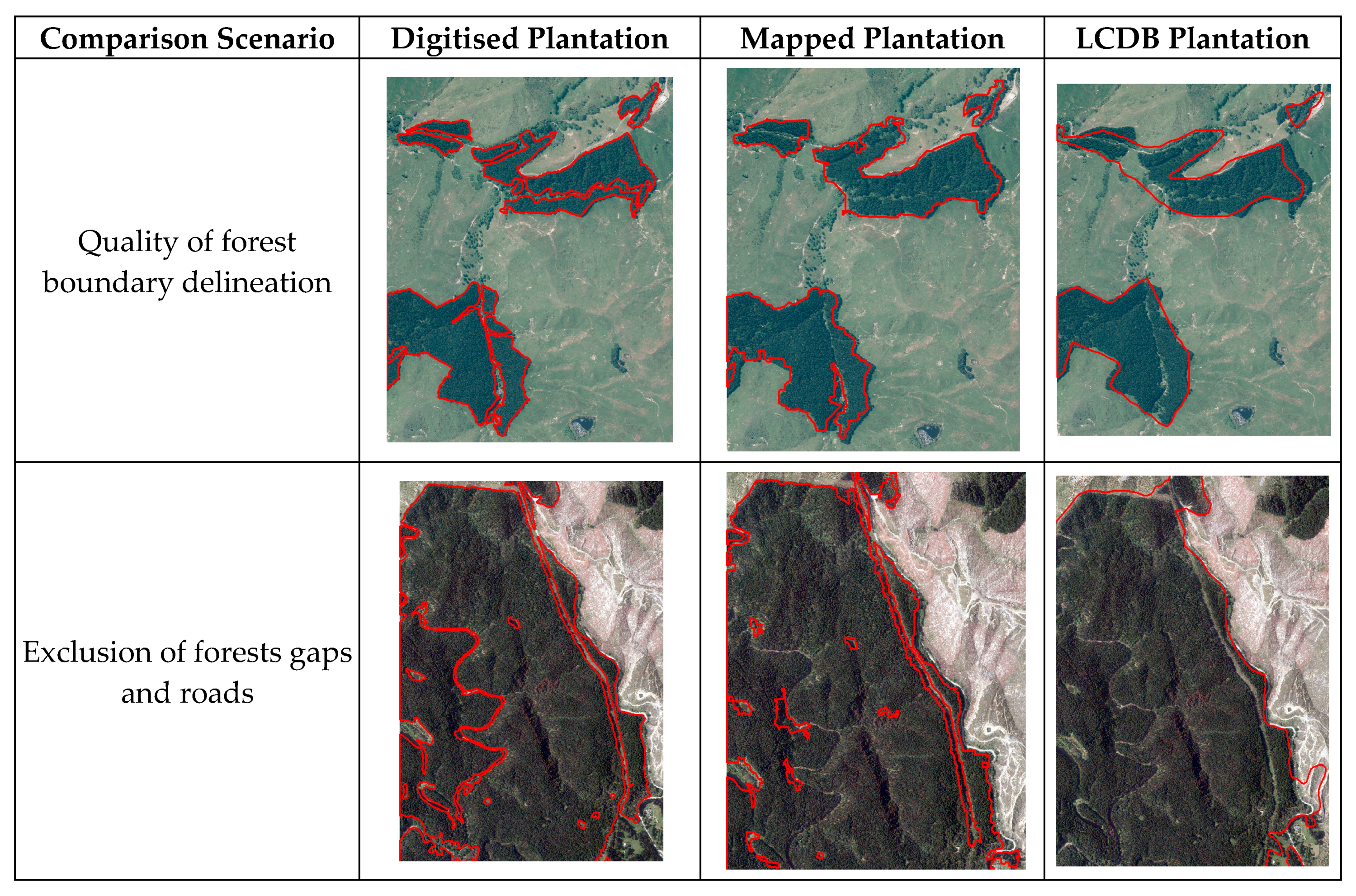
Figure 6 provides a visual comparison of the plantation area mapped by manual digitisation, the automated mapping approach, and the LCDB mapped plantation area for reference. Using the mapping approach with RapidEye and LiDAR data, plantations and forest gaps were able to be mapped with a high degree of certainty, relative to LCDB. LCDB provides reasonable means for detecting and summarising plantation area, but with the limitation in resolution, LCDB may not be suitable for providing accurate estimation of plantation area at small-scales.
3.5. Patch-Level Plantation Area Comparison
Patch-level comparison was conducted to examine whether the accuracy of the classification approach varies with the size of plantation patch. For all patch-level comparisons, with an average digitised patch size of 9.5 ha, the mapping approach tends to overestimate plantation area by 2.1% with a mean absolute error of 0.8 ha (Table 9). For forest patches under one hectare, with an average digitised patch size of 0.3 ha, mapping appears to be less accurate, overestimating plantation area by 8.2%, with a mean absolute error of 0.3 ha. However, the total area of these patches is small, so the relatively large error in small plantation patch estimation only caused 8.9 ha over estimation for all grids (Table 9). On the other hand, although forest patches exceeding one hectare were only overestimated by 1.9% (MAE = 1.46 ha), the errors associated with these patches were the main contributor to the overall error. The above comparisons include forest patches not mapped or digitised, which means that if a forest patch was digitised but not mapped, the mapped area is recorded as zero.
A paired two-tail t-test was used to determine whether the difference between the mean area of digitised forest patches and mapped forest patches is significant. The absolute value of t statistics for all patches and >1 ha patches were marginally larger (t = 2.011) than the critical two-tail t value (t = 1.969) and the p-value is 0.045, which suggests that the average patch size mapped and digitised are marginally and statistically different. However, t-tests on <1 ha patches were not significant (t = 0.959, p = 0.338). This suggests that there was no obvious difference in the average patch size digitised and mapped for less than 1 ha patches.
In order to further visualise the digitised and mapped plantations, only non-zero comparisons were used in the plot of the mapped and digitised plantation. That excludes 142 polygons missed by mapping and 22 polygons missed by digitisation, leaving 423 sets of non-zero comparisons. The digitised and mapped plantation areas at patch-level are plotted in Figure 7. The graph shows that digitised and mapped patch areas closely correlate, especially for larger forest patches. Smaller patches appear more difficult to map accurately as there are more discrepancies in areas for smaller areas.
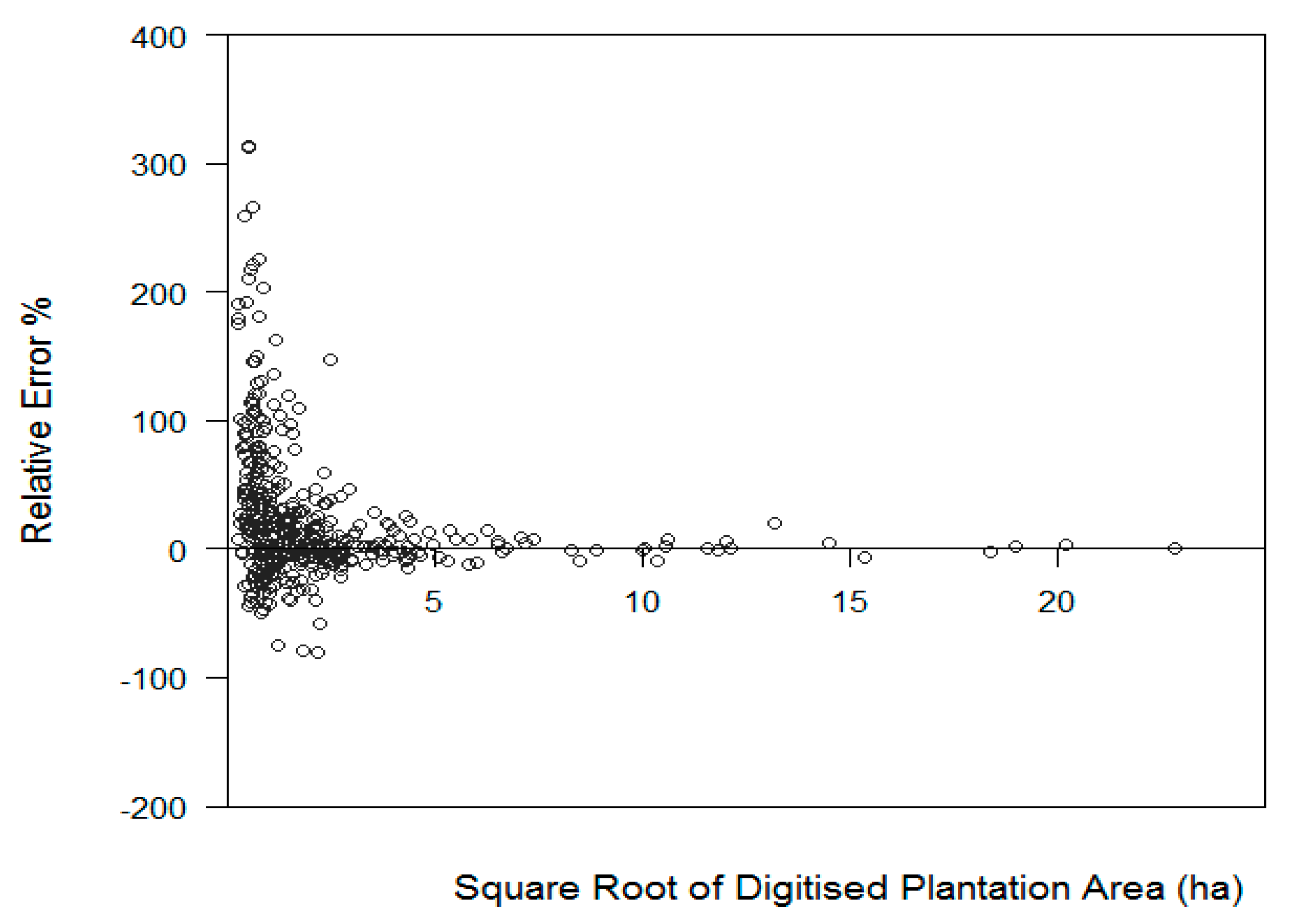
Figure 8 confirms previous observations by plotting the absolute error with patch size, which shows that errors tend to decrease with increasing patch size. The mapping errors appear to be greater and have more variability for smaller forest patches, whereas forest patches that exceed 10 ha, the errors become much smaller and less variable (within 20% error).
4. Conclusions
In this study, a factorial combination of two classification approaches and two remote sensing datasets were compared for their ability to accurately classify land cover, specifically plantation forest area. The approaches included nearest neighbour with RapidEye only, nearest neighbour with RapidEye and LiDAR, CART with RapidEye and CART with RapidEye and LiDAR. In an initial classification of nine training grids, CART with RapidEye and LiDAR outperformed the other three approaches, producing the highest overall accuracy and plantation accuracy. The addition of LiDAR data to RapidEye has improved the overall classification accuracy by 8% using the CART approach, and the producer’s accuracy of planted forest improved by 7% compared to using RapidEye images alone. Therefore, the CART approach with both RapidEye and LiDAR was chosen for land cover mapping in the remaining 60 validation grids.
Overall, the selected mapping approach gave good classification results, producing 89% overall accuracy; the producer’s accuracy for plantation was 79% and user’s accuracy was 94%. After excluding the harvested area and new plantings due to temporal differences between the aerial photography and satellite imagery, the producer’s accuracy of plantation increased to 89%. The mapping approach used here has produced classification results comparable to previous studies [9,13,23,28,49]. The accuracy of the method was further examined by comparing the mapped plantation area with manually digitised plantation area. For all sample grids, the mapping approach overestimated the total plantation area by 7.8%, and overestimated the plantation area excluding new plantings by 3%. Patch size proved to have an impact on mapping accuracy. Mapping of smaller patches (less than 10 ha) appears more variable and less accurate compared to “true” representation, whereas larger patches (over 10 ha) are generally more accurately mapped (less than 20% error).
The combination of multispectral RapidEye features and relatively low point density LiDAR-derived surfaces proved to be sufficient to detect land cover features, though the mapping accuracy decreased in small plantation patches. Another limitation with the mapping approach was that it failed to detect young plantings due to the resolution of remote sensing datasets. Together with the reduced accuracy for mapping forest patches smaller than 10 ha, this limitation hints at the relationship between mapping accuracy and the spatial resolution of the input data.
Though we did not test the effects of differing spatial resolutions in this study, other studies have generally shown improved forest mapping accuracy with higher spatial resolution datasets. For example, the average accuracy of urban forest species classification was increased by 16–18% using 2-m Worldview2 compared with using 4-m IKONOS [55]. Another example showed that using grids derived from higher LiDAR point density (5 points m−1) could produce 96% overall accuracy for delineating forested areas in a coniferous forest in Austria [56].
A future study to test the accuracy of differing small-scale forest mapping approaches with input imagery of varying spatial resolutions would be useful. Such a study would improve the chances of successfully applying the automated mapping approach developed here over larger areas, for which RapidEye imagery and LiDAR data are not readily available. In such instances, freely available imagery (e.g., Landsat, Sentinel-2) have commonly been used for forest mapping. A spatial resolution sensitivity analysis, as proposed above, would help to determine the utility of such freely-available imagery for small-scale forest mapping. In addition, applying small-scale forest mapping approaches over a time series of imagery would be useful for offsetting the spatial resolution constraint.
In conclusion, the mapping approach developed in this study provides a proof of concept for estimating plantation area using remotely sensed data in the Wairarapa region of New Zealand, and the enhanced area description of small-scale forests will allow more effective planning for the forest industry.
Supplementary Materials
The following are available online at www.mdpi.com/1999-4907/8/12/487/s1.
Acknowledgments
Thanks to the funding provided by the New Zealand School of Forestry—PhD Scholarship, T. W. Adams and Owen Browning Scholarships. Acknowledgements to the Greater Wellington Region and Landcare Research for providing the LiDAR data; Indufor Asia Pacific and Blackbridge Ltd. for providing the RapidEye images; and Land Information New Zealand for providing the aerial photography required for this research.
Author Contributions
Cong Xu performed all the preparation of data, classification and analysis of results, and write up of the paper. Justin Morgenroth provided guidance on remote sensing data analysis and classification; Bruce Manley contributed to the area comparison analysis. Both Justin Morgenroth and Bruce Manley reviewed the draft paper.
Conflicts of Interest
The authors declare no conflict of interest.
References
- The New Zealand Forest Owners Association (NZFOA). Facts and Figures 2015/16 New Zealand Plantation Forest Industry; New Zealand Forest Owners Association: Wellington, New Zealand, 2016. [Google Scholar]
- Ministry of Primary Industries (MPI). 2016 National Exotic Forest Description; Ministry of Primary Industries: Wellington, New Zealand, 2016.
- Manley, B.; Somerville, O.; Turbitt, M.; Lane, P. Review of new forest planting estimates. N. Z. J. For. 2003, 48, 34–37. [Google Scholar]
- Ministry of Primary Industries (MPI). Wood Availability Forecasts—New Zealand 2014‒2050; Ministry of Primary Industries: Wellington, New Zealand, 2016.
- Ministry for the Environment (MfE). New Zealand Land Cover Database 2 User Guide; Ministry for the Environment: Wellington, New Zealand, 2004.
- Mustonen, J.; Packalén, P.; Kangas, A. Automatic segmentation of forest stands using a canopy height model and aerial photography. Scand. J. For. Res. 2008, 23, 534–545. [Google Scholar] [CrossRef]
- Deo, R.K.; Russell, M.B.; Domke, G.M.; Woodall, C.W.; Falkowski, M.J.; Cohen, W.B. Using landsat time-series and lidar to inform aboveground forest biomass baselines in northern minnesota, USA. Can. J. Remote Sens. 2017, 43, 28–47. [Google Scholar] [CrossRef]
- Bork, E.W.; Su, J.G. Integrating lidar data and multispectral imagery for enhanced classification of rangeland vegetation: A meta analysis. Remote Sens. Environ. 2007, 111, 11–24. [Google Scholar] [CrossRef]
- Nordkvist, K.; Granholm, A.H.; Holmgren, J.; Olsson, H.; Nilsson, M. Combining optical satellite data and airborne laser scanner data for vegetation classification. Remote Sens. Lett. 2012, 3, 393–401. [Google Scholar] [CrossRef]
- Hudak, A.T.; Evans, J.S.; Smith, A.M.S. Lidar utility for natural resource managers. Remote Sens. 2009, 1, 934–951. [Google Scholar] [CrossRef]
- Deo, R.K.; Froese, R.E.; Falkowski, M.J.; Hudak, A.T. Optimizing variable radius plot size and lidar resolution to model standing volume in conifer forests. Can. J. Remote Sens. 2016, 42, 428–442. [Google Scholar] [CrossRef]
- Xu, C.; Morgenroth, J.; Manley, B. Integrating data from discrete return airborne lidar and optical sensors to enhance the accuracy of forest description: A review. Curr. For. Rep. 2015, 1, 206–219. [Google Scholar] [CrossRef]
- Sasaki, T.; Imanishi, J.; Ioki, K.; Morimoto, Y.; Kitada, K. Object-based classification of land cover and tree species by integrating airborne lidar and high spatial resolution imagery data. Landsc. Ecol. Eng. 2012, 8, 157–171. [Google Scholar] [CrossRef]
- Sasaki, T.; Imanishi, J.; Ioki, K.; Morimoto, Y.; Kitada, K. Estimation of leaf area index and canopy openness in broad-leaved forest using an airborne laser scanner in comparison with high-resolution near-infrared digital photography. Landsc. Ecol. Eng. 2008, 4, 47–55. [Google Scholar] [CrossRef]
- Blaschke, T. Object based image analysis for remote sensing. ISPRS J. Photogramm. Remote Sens. 2010, 65, 2–16. [Google Scholar] [CrossRef]
- Lu, D.; Weng, Q. A survey of image classification methods and techniques for improving classification performance. Int. J. Remote Sens. 2007, 28, 823–870. [Google Scholar] [CrossRef]
- Chubey, M.S.; Franklin, S.E.; Wulder, M.A. Object-based analysis of ikonos-2 imagery for extraction of forest inventory parameters. Photogramm. Eng. Remote Sens. 2006, 72, 383–394. [Google Scholar] [CrossRef]
- Myint, S.W.; Gober, P.; Brazel, A.; Grossman-Clarke, S.; Weng, Q. Per-pixel vs. Object-based classification of urban land cover extraction using high spatial resolution imagery. Remote Sens. Environ. 2011, 115, 1145–1161. [Google Scholar] [CrossRef]
- Tehrany, M.S.; Pradhan, B.; Jebuv, M.N. A comparative assessment between object and pixel-based classification approaches for land use/land cover mapping using spot 5 imagery. Geocarto Int. 2014, 29, 351–369. [Google Scholar] [CrossRef]
- Whiteside, T.G.; Boggs, G.S.; Maier, S.W. Comparing object-based and pixel-based classifications for mapping savannas. Int. J. Appl. Earth Obs. Geoinform. 2011, 13, 884–893. [Google Scholar] [CrossRef]
- Hubert-Moy, L.; Cotonnec, A.; Le Du, L.; Chardin, A.; Perez, P. A comparison of parametric classification procedures of remotely sensed data applied on different landscape units. Remote Sens. Environ. 2001, 75, 174–187. [Google Scholar] [CrossRef]
- Mallinis, G.; Koutsias, N.; Tsakiri-Strati, M.; Karteris, M. Object-based classification using quickbird imagery for delineating forest vegetation polygons in a mediterranean test site. ISPRS J. Photogramm. Remote Sens. 2008, 63, 237–250. [Google Scholar] [CrossRef]
- Machala, M.; Zejdova, L. Forest mapping through object-based image analysis of multispectral and lidar aerial data. Eur. J. Remote Sens. 2014, 47, 117–131. [Google Scholar] [CrossRef]
- Haapanen, R.; Ek, A.R.; Bauer, M.E.; Finley, A.O. Delineation of forest/nonforest land use classes using nearest neighbor methods. Remote Sens. Environ. 2004, 89, 265–271. [Google Scholar] [CrossRef]
- Ohmann, J.L.; Gregory, M.J. Predictive mapping of forest composition and structure with direct gradient analysis and nearest-neighbor imputation in coastal oregon, USA. Can. J. For. Res. 2002, 32, 725–741. [Google Scholar] [CrossRef]
- Breiman, L.; Friedman, J.; Stone, C.J.; Olshen, R.A. Classification and Regression Trees; Wadsworth International Group: Belmont, CA, USA, 1984. [Google Scholar]
- Trimble. Ecognition Developer 8.9 User Guide; Trimble: Sunnyvale, CA, USA, 2013. [Google Scholar]
- Hellesen, T.; Matikainen, L. An object-based approach for mapping shrub and tree cover on grassland habitats by use of lidar and cir orthoimages. Remote Sens. 2013, 5, 558–583. [Google Scholar] [CrossRef]
- Planet Labs. Rapideye™ Imagery Product Specifications. Available online: https://www.planet.com/products/satellite-imagery/files/160625-RapidEye%20Image-Product-Specifications.pdf (accessed on 15 May 2016).
- Schrader, B. Wairarapa region—Land and climate. In Te Ara—The Encyclopedia of New Zealand; Ministry for Culture and Heritage: Wellington, New Zealand, 2017. [Google Scholar]
- Richter, R.; Schläpfer, D. Atmospheric/topographic correction for satellite imagery. In ATCOR 2/3 User Guide, version 8.3.1; ReSe Applications Schläpfer: Langeggweg, Switzerland, 2014. [Google Scholar]
- Berk, A.; Bernstein, L.S.; Anderson, G.P.; Acharya, P.K.; Robertson, D.C.; Chetwynd, J.H.; Adler-Golden, S.M. Modtran cloud and multiple scattering upgrades with application to aviris. Remote Sens. Environ. 1998, 65, 367–375. [Google Scholar] [CrossRef]
- Berk, A.; Anderson, G.P.; Acharya, P.K.; Shettle, E.P. Modtran® 5.2.0.0 User’s Manual; Air Force Research Laboratory Spectral Sciences Inc.: Burlington MA, USA, 2008. [Google Scholar]
- Balthazar, V.; Vanacker, V.; Lambin, E.F. Evaluation and parameterization of atcor3 topographic correction method for forest cover mapping in mountain areas. Int. J. Appl. Earth Obs. Geoinform. 2012, 18, 436–450. [Google Scholar] [CrossRef]
- Hantson, S.; Chuvieco, E. Evaluation of different topographic correction methods for landsat imagery. Int. J. Appl. Earth Obs. Geoinform. 2011, 13, 691–700. [Google Scholar] [CrossRef]
- Richter, R.; Kellenberger, T.; Kaufmann, H. Comparison of topographic correction methods. Remote Sens. 2009, 1, 184–196. [Google Scholar] [CrossRef] [Green Version]
- Columbus, J.; Sirguey, P.; Tenzer, R. A free fully assessed 15 m digital elevation model for new zealand. Surv. Q. 2011, 300, 16–19. [Google Scholar]
- Rosner, B. Hypothesis testing: Categorical data—estimation of sample size and power for comparing two binomial proportions. In Fundamentals of Biostatistics, 7th ed.; Brooks/Cole, Cengage Learning: Boston, MA, USA, 2011. [Google Scholar]
- Drăguţ, L.; Csillik, O.; Eisank, C.; Tiede, D. Automated parameterisation for multi-scale image segmentation on multiple layers. ISPRS J. Photogramm. Remote Sens. 2014, 88, 119–127. [Google Scholar] [CrossRef] [PubMed]
- Drăguţ, L.; Tiede, D.; Levick, S.R. Esp: A tool to estimate scale parameter for multiresolution image segmentation of remotely sensed data. Int. J. Geogr. Inf. Sci. 2010, 24, 859–871. [Google Scholar] [CrossRef]
- Haralick, R.M.; Shanmugam, K. Textural features for image classification. IEEE Trans. Syst. Man Cybern. 1973, 610–621. [Google Scholar] [CrossRef]
- Rana, P.; Tokola, T.; Korhonen, L.; Xu, Q.; Kumpula, T.; Vihervaara, P.; Mononen, L. Training area concept in a two-phase biomass inventory using airborne laser scanning and rapideye satellite data. Remote Sens. 2014, 6, 285–309. [Google Scholar] [CrossRef]
- Blanchard, S.D.; Jakubowski, M.K.; Kelly, M. Object-based image analysis of downed logs in disturbed forested landscapes using lidar. Remote Sens. 2011, 3, 2420–2439. [Google Scholar] [CrossRef]
- Trimble. Ecognition Developer 8.9 Reference Book; Trimble: Sunnyvale, CA, USA, 2013. [Google Scholar]
- Congalton, R.G. A review of assessing the accuracy of classifications of remotely sensed data. Remote Sens. Environ. 1991, 37, 35–46. [Google Scholar] [CrossRef]
- Congalton, R.G.; Green, K. Sample design considerations. In Assessing the Accuracy of Remotely Sensed Data; CRC Press: Boca Raton, FL, USA, 2008; pp. 63–83. [Google Scholar]
- Plourde, L.; Congalton, R.G. Sampling method and sample placement: How do they affect the accuracy of remotely sensed maps? Photogramm. Eng. Remote Sens. 2003, 69, 289–297. [Google Scholar] [CrossRef]
- Xu, C. Obtaining Forest Description for Small-Scale Forests Using an Integrated Remote Sensing Approach. Ph.D. Thesis, University of Canterbury Christchurch, Christchurch, New Zealand, 2017. [Google Scholar]
- Haywood, A.; Stone, C. Semi-automating the stand delineation process in mapping natural eucalpt forest. Aust. For. 2009, 74, 13–22. [Google Scholar] [CrossRef]
- Pham, L.T.H.; Brabyn, L.; Ashraf, S. Combining quickbird, lidar, and gis topography indices to identify a single native tree species in a complex landscape using an object-based classification approach. Int. J. Appl. Earth Obs. Geoinform. 2016, 50, 187–197. [Google Scholar] [CrossRef]
- Dupuy, S.; Laine, G.; Tassin, J.; Sarrailh, J.M. Characterization of the horizontal structure of the tropical forest canopy using object-based lidar and multispectral image analysis. Int. J. Appl. Earth Obs. Geoinform. 2013, 25, 76–86. [Google Scholar] [CrossRef]
- Räsänen, A.; Kuitunen, M.; Tomppo, E.; Lensu, A. Coupling high-resolution satellite imagery with als-based canopy height model and digital elevation model in object-based boreal forest habitat type classification. ISPRS J. Photogramm. Remote Sens. 2014, 94, 169–182. [Google Scholar] [CrossRef]
- Zhou, J.; Proisy, C.; Descombes, X.; le Maire, G.; Nouvellon, Y.; Stape, J.-L.; Viennois, G.; Zerubia, J.; Couteron, P. Mapping local density of young eucalyptus plantations by individual tree detection in high spatial resolution satellite images. For. Ecol. Manag. 2013, 301, 129–141. [Google Scholar] [CrossRef] [Green Version]
- Landcare Research. Lcdb v4.1—Land Cover Database Version 4.1. Available online: https://lris.scinfo.org.nz/layer/423-lcdb-v41-land-cover-database-version-41-mainland-new-zealand/ (accessed on 20 August 2016).
- Pu, R.L.; Landry, S. A comparative analysis of high spatial resolution ikonos and worldview-2 imagery for mapping urban tree species. Remote Sens. Environ. 2012, 124, 516–533. [Google Scholar] [CrossRef]
- Eysn, L.; Hollaus, M.; Schadauer, K.; Pfeifer, N. Forest delineation based on airborne lidar data. Remote Sens. 2012, 4, 762–783. [Google Scholar] [CrossRef]
Figure 1.
Study location.

Figure 2.
Sample grid selection and distribution of forest type.

Figure 3.
Mapping process workflow.

Figure 4.
Example showing classification errors caused by change. The image on the left shows a plantation patch on an aerial photo, on the right the same area was shown to be harvested on RapidEye imagery, which would be classified as bare ground.
Figure 4.
Example showing classification errors caused by change. The image on the left shows a plantation patch on an aerial photo, on the right the same area was shown to be harvested on RapidEye imagery, which would be classified as bare ground.
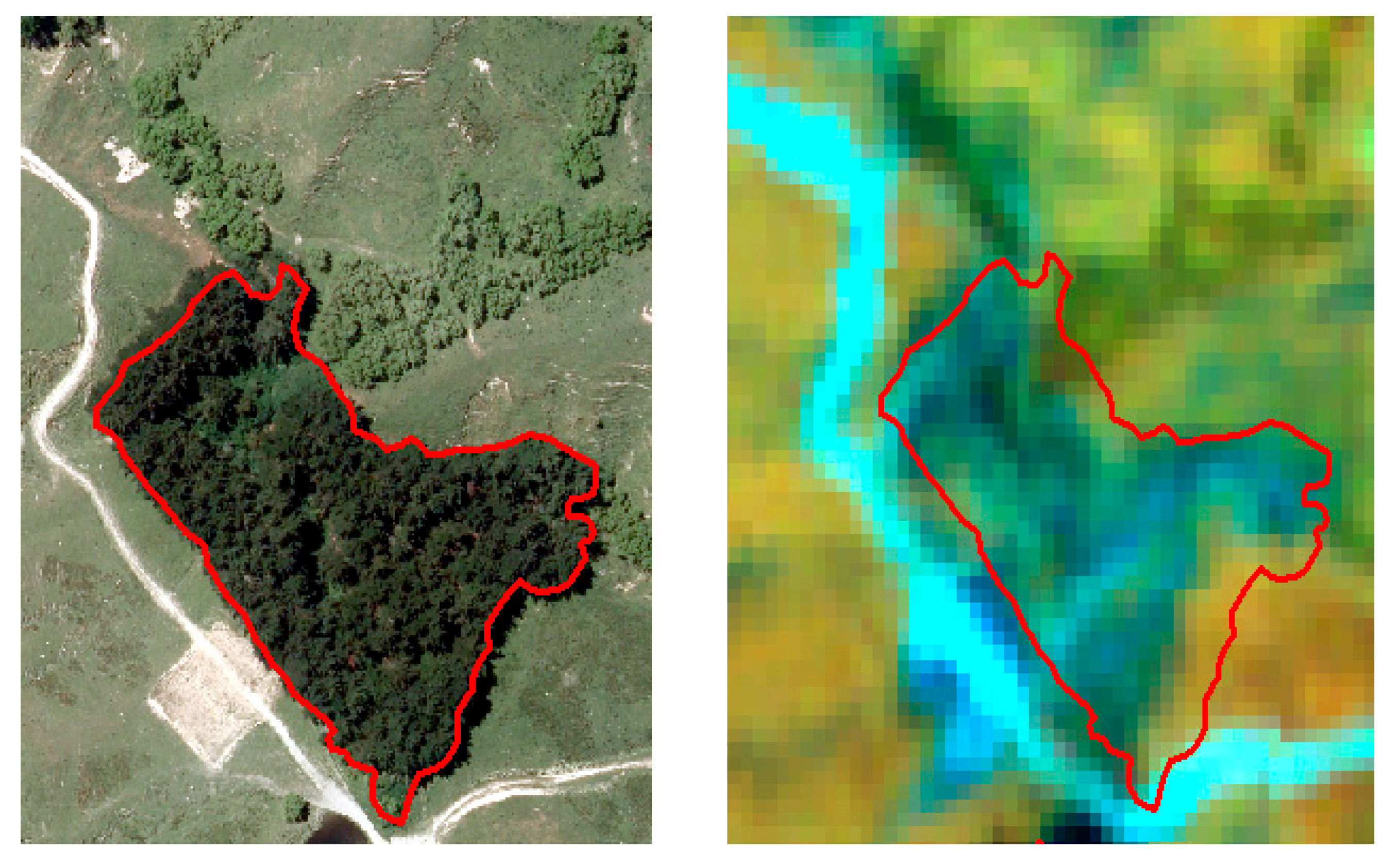
Figure 5.
Example showing the different classification caused by image pixel size. The point on the left image shows a road within a natural forest on an aerial photo, which was classed as “bare ground” by the operator. The image on the right shows the same area on RapidEye, which was classified as natural forest as the coarser pixel size resulted in the road not being classified by the automated classification approach on RapidEye.
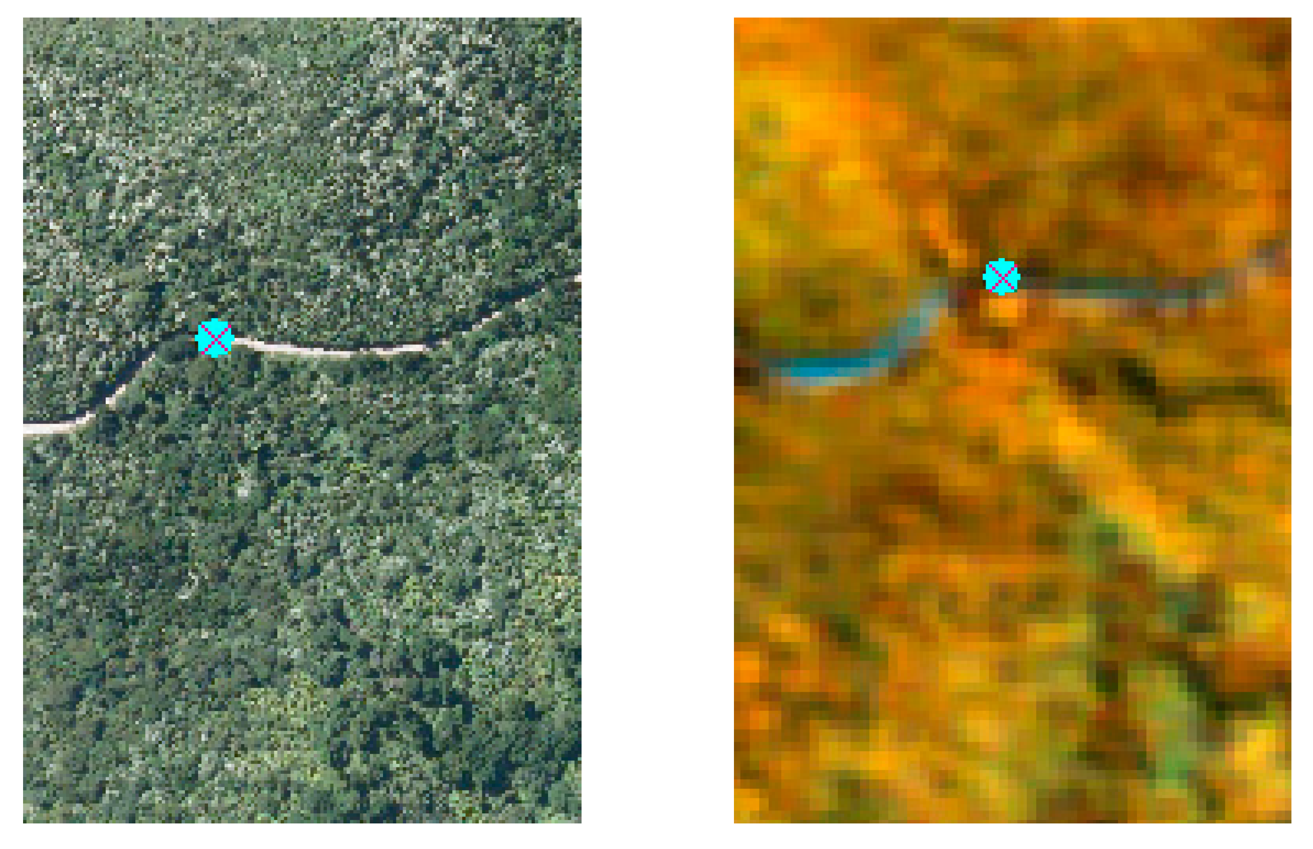
Figure 6.
Visual examples of plantation mapped in comparison to digitised plantation and Land Cover Database (LCDB) plantation.
Figure 6.
Visual examples of plantation mapped in comparison to digitised plantation and Land Cover Database (LCDB) plantation.

Figure 7.
Plot of digitised mapped plantation areas, with logarithm transformation at base of 10 due to wide range of input values. The R2 of the linear correlation was 0.95. The trend line is a 1:1 line.
Figure 7.
Plot of digitised mapped plantation areas, with logarithm transformation at base of 10 due to wide range of input values. The R2 of the linear correlation was 0.95. The trend line is a 1:1 line.
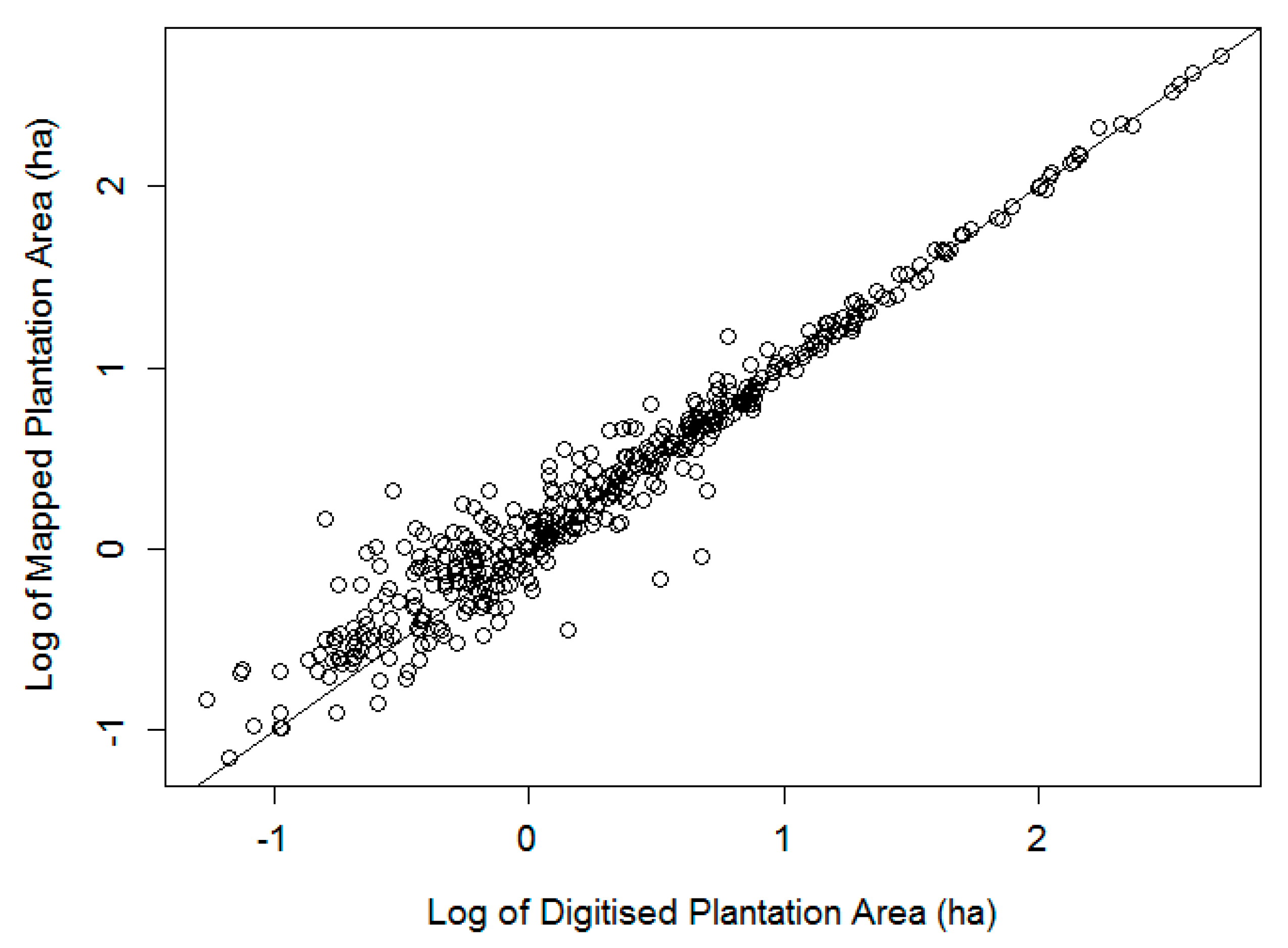
Figure 8.
Plot of forest patch size against mapping error, forest patch size is expressed as square root of digitised plantation area, error is expressed as the relative error percentage which was calculated as the difference of mapped and digitised area divided by the digitised area.
Figure 8.
Plot of forest patch size against mapping error, forest patch size is expressed as square root of digitised plantation area, error is expressed as the relative error percentage which was calculated as the difference of mapped and digitised area divided by the digitised area.


Table 1.
LiDAR Survey Specification.
| LiDAR Attributes | Details |
|---|---|
| Scanner | Optech ALTM 3100EA |
| Flying Height | 1000 m |
| Scan Angle | ±18.8° |
| Scan Frequency | 53 Hz |
| Pulse Rate | 100 kHz |
| Swath Overlap | 50% |
| Swath Width | 680 m |
| Point density | 3.76 points m−2 |
Table 2.
Parameters used in multi-resolution segmentation.
| Forest Class | Scale | Shape | Compactness | Image Weight | |
|---|---|---|---|---|---|
| RapidEye | 1 | 100 | 0.2 | 0.5 | Red, Green, Blue, RedEdge: 1, NIR: 2 |
| 2 | 120 | 0.2 | 0.5 | Red, Green, Blue, RedEdge: 1, NIR: 2 | |
| 3 | 140 | 0.2 | 0.5 | Red, Green, Blue, RedEdge: 1, NIR: 2 | |
| RapidEye+LiDAR | 1 | 100 | 0.2 | 0.5 | Red, Green, Blue, RedEdge: 1, NIR, CHM: 2 |
| 2 | 120 | 0.2 | 0.5 | Red, Green, Blue, RedEdge: 1, NIR, CHM: 2 | |
| 3 | 140 | 0.2 | 0.5 | Red, Green, Blue, RedEdge: 1, NIR, CHM: 2 |
Table 3.
Description of land cover classes.
| Land Class | Description |
|---|---|
| Bare ground | Land that is exposed with no vegetation, e.g., Roads, harvested area |
| Grassland | Natural high and low tussock grassland |
| Natural Forest | Closed naturally generated forests, e.g., Kauri, rimu, tōtara, native beech forests |
| Planted Forest | Closed planted forests, e.g., radiata pine plantations |
| Shrubland and scrub | Open forest (low density), riparian vegetation, both indigenous and exotic scrub |
| Water | River and lake, including shores |
| Features | Description |
|---|---|
| BlueRatio | blue/(blue+green+red+re+nir) |
| EVI | 2.5((nir-red)/(nir+6red-7.5blue+1)) |
| Green/Blue | green/blue |
| Green/Red | green/red |
| GreenRatio | green/(blue+green+red+re+nir) |
| GreenXRE/Red | green*re/red |
| NDVI | (nir-red)/(nir+red) |
| NIR/Blue | nir/blue |
| NIR/Green | nir/green |
| NIR/Red | nir/red |
| NIR/RedSDRatio | (nir*StDev nir)/(red*StDev nir) |
| NIRRatio | nir/(blue+green+red+re+nir) |
| RedRatio | red/(blue+green+red+re+nir) |
| REGNDVI | (re-green)/(re+green) |
| RENDVI | (re-red)/(re+red) |
| RERatio | re/(blue+green+red+re+nir) |
| 3bandratio | nir/red/green |
Table 5.
Classification accuracy comparison among classification approach and datasets for nine training grids.
Table 5.
Classification accuracy comparison among classification approach and datasets for nine training grids.
| NN-RE | NN-RE+LiDAR | CART-RE | CART-RE+LiDAR | |||||
|---|---|---|---|---|---|---|---|---|
| Land Cover | Producer’s Accuracy | User’s Accuracy | Producer’s Accuracy | User’s Accuracy | Producer’s Accuracy | User’s Accuracy | Producer’s Accuracy | User’s Accuracy |
| Bare ground | 40% | 20% | 40% | 23% | 43% | 20% | 38% | 26% |
| Grassland | 59% | 90% | 60% | 89% | 69% | 91% | 76% | 90% |
| Natural Forest | 52% | 39% | 65% | 46% | 68% | 50% | 67% | 71% |
| Planted Forest | 80% | 83% | 82% | 86% | 81% | 94% | 88% | 90% |
| Shrubland and scrub | 55% | 34% | 58% | 40% | 46% | 41% | 77% | 55% |
| Water | 80% | 21% | 80% | 21% | 70% | 16% | 90% | 26% |
| Overall Accuracy | 60% | 63% | 67% | 75% | ||||
Table 6.
Classification accuracy matrix for nine training grids using the refined mapping approach.
| Classes | Reference Data | Total | User’s Accuracy | |||||
|---|---|---|---|---|---|---|---|---|
| Bare Ground | Grassland | Natural Forest | Planted Forest | Shrubs and Scrub | Water | |||
| Bare ground | 27 | 16 | 1 | 2 | 1 | 1 | 48 | 56% |
| Grassland | 24 | 571 | 7 | 6 | 13 | 0 | 621 | 92% |
| Natural Forest | 5 | 15 | 127 | 14 | 19 | 0 | 180 | 71% |
| Planted Forest | 0 | 4 | 8 | 175 | 4 | 0 | 191 | 92% |
| Shrubland and scrub | 1 | 17 | 17 | 0 | 113 | 0 | 148 | 76% |
| Water | 3 | 0 | 0 | 0 | 0 | 9 | 12 | 75% |
| Total | 60 | 623 | 160 | 197 | 150 | 10 | 1200 | |
| Producer’s Accuracy | 45% | 92% | 79% | 89% | 75% | 90% | 85% | |
Table 7.
Classification accuracy matrix for 60 validation grids, the values in parentheses show the updated classification accuracy when excluding errors caused by temporal differences between RapidEye and aerial photography.
Table 7.
Classification accuracy matrix for 60 validation grids, the values in parentheses show the updated classification accuracy when excluding errors caused by temporal differences between RapidEye and aerial photography.
| Classification | Reference | Total | User’s Accuracy | |||||
|---|---|---|---|---|---|---|---|---|
| Bare Ground | Grassland | Natural Forest | Planted Forest | Shrubland and Scrub | Water | |||
| Bare ground | 23 | 6 (1) | 0 | 4 (1) | 1 | 3 (2) | 37 (28) | 62% (82%) |
| Grassland | 7 (0) | 641 | 8 | 6 (0) | 14 | 1 | 677 (664) | 95% (97%) |
| Natural Forest | 0 | 8 | 141 | 11 | 17 | 0 | 177 | 80% |
| Planted Forest | 0 | 0 | 6 | 131 | 2 | 0 | 139 | 94% |
| Shrubland and scrub | 1 | 16 (14) | 11 | 13 (4) | 111 | 0 | 152 (141) | 73% (79%) |
| Water | 0 | 0 | 0 | 0 | 0 | 18 | 18 | 100% |
| Total | 31 (24) | 671 (664) | 166 | 165 (147) | 145 | 22 (21) | 1200 (1167) | |
| Producer’s Accuracy | 74% (96%) | 96% (97%) | 85% | 79% (89%) | 77% | 82% (86%) | 89% (91%) | |
Table 8.
Overall area comparison between planted forests mapped by mapping approach and digitised from aerial photography, based on both the nine test grids and 60 validation grids.
Table 8.
Overall area comparison between planted forests mapped by mapping approach and digitised from aerial photography, based on both the nine test grids and 60 validation grids.
| Total Digitised (ha) | Total Mapped (ha) | Difference (ha) | Difference (%) | MAE (ha) | RMSE (ha) | |
|---|---|---|---|---|---|---|
| All standing trees | 6244.4 | 5759.2 | −485.2 | −7.8% | 13.6 | 42.5 |
| Exclude new plantings | 5590.8 | 5759.2 | 168.5 | 3.0% | 5.7 | 9.6 |
Table 9.
Patch-level comparison summary.
| Digitised Plantation Area (ha) | Average Digitised Patch Size (ha) | Mapped Plantation Area (ha) | Difference Mapped/Digitised (ha) | Difference Mapped/Digitised (%) | MAE (ha) | RMSE (ha) | |
|---|---|---|---|---|---|---|---|
| All | 5557.1 | 9.5 | 5671.3 | 114.2 | 2.1% | 0.8 | 2.3 |
| <1 ha | 109.2 | 0.3 | 118.1 | 8.9 | 8.2% | 0.3 | 0.4 |
| >1 ha | 5447.9 | 20.3 | 5553.2 | 105.3 | 1.9% | 1.5 | 3.4 |
© 2017 by the authors. Licensee MDPI, Basel, Switzerland. This article is an open access article distributed under the terms and conditions of the Creative Commons Attribution (CC BY) license (http://creativecommons.org/licenses/by/4.0/).
Share and Cite
MDPI and ACS Style
Xu, C.; Morgenroth, J.; Manley, B. Mapping Net Stocked Plantation Area for Small-Scale Forests in New Zealand Using Integrated RapidEye and LiDAR Sensors. Forests 2017, 8, 487. https://doi.org/10.3390/f8120487
AMA Style
Xu C, Morgenroth J, Manley B. Mapping Net Stocked Plantation Area for Small-Scale Forests in New Zealand Using Integrated RapidEye and LiDAR Sensors. Forests. 2017; 8(12):487. https://doi.org/10.3390/f8120487
Chicago/Turabian StyleXu, Cong, Justin Morgenroth, and Bruce Manley. 2017. "Mapping Net Stocked Plantation Area for Small-Scale Forests in New Zealand Using Integrated RapidEye and LiDAR Sensors" Forests 8, no. 12: 487. https://doi.org/10.3390/f8120487
Note that from the first issue of 2016, this journal uses article numbers instead of page numbers. See further details here.