Assessing Wildland Fire Risk Transmission to Communities in Northern Spain

Abstract

We assessed potential economic losses and transmission to residential houses from wildland fires in a rural area of central Navarra (Spain). Expected losses were quantified at the individual structure level (n = 306) in 14 rural communities by combining fire model predictions of burn probability and fire intensity with susceptibility functions derived from expert judgement. Fire exposure was estimated by simulating 50,000 fire events that replicated extreme (97th percentile) historical fire weather conditions. Spatial ignition probabilities were used in the simulations to account for non-random ignitions, and were estimated from a fire occurrence model generated with an artificial neural network. The results showed that ignition probability explained most of spatial variation in risk, with economic value of structures having only a minor effect. Average expected loss to residential houses from a single wildfire event in the study area was 7955€, and ranged from a low of 740 to the high of 28,725€. Major fire flow-paths were analyzed to understand fire transmission from surrounding municipalities and showed that incoming fires from the north exhibited strong pathways into the core of the study area, and fires spreading from the south had the highest likelihood of reaching target residential structures from the longest distances (>5 km). Community firesheds revealed the scale of risk to communities and extended well beyond administrative boundaries. The results provided a quantitative risk assessment that can be used by insurance companies and local landscape managers to prioritize and allocate investments to treat wildland fuels and identify clusters of high expected loss within communities. The methodological framework can be extended to other fire-prone southern European Union countries where communities are threatened by large wildland fires.

1. Introduction

Most wildfires that cause human fatalities and losses to property occur in the rapidly expanding interface areas between wildlands and human development [1,2]. This area where residential and other infrastructures intermingle with flammable vegetation is widely known as wildland–urban interface (WUI) or rural–urban interface (RUI) [3,4]. While the former definition is mainly used for predominantly wildland vegetation areas surrounding developed areas, the latter is most commonly used in Mediterranean landscapes where fuels have been influenced by human activities for millennia [5,6]. In areas lacking sharp transitions between development and wildlands, where structures are surrounded by hazardous fuels, the term intermix has been used to describe the juxtaposition of fuels and dwellings [7]. In all cases, a number of factors have contributed to wildfire losses in developed areas (hereafter WUI), including urban expansion, increased fuel loadings from expansion of shrub and forest vegetation into abandoned agricultural lands, and suburban sprawl over metropolitan agricultural belts [8,9,10]. Likewise, fire suppression policies have contributed to a buildup of fuels in and around developed areas, resulting in higher hazard within developed areas and structure ignition [11]. Wildland fires in the WUI are a growing concern at global scales due to escalating losses to life and property [12,13], and have become a priority for wildfire management policies in many fire-prone areas [14].

Previous efforts on WUI wildfire risk characterization in Mediterranean landscapes have emphasized the importance of flammable vegetation surrounding communities [15], since fuel loadings are directly related to fire intensity and structure loss [16]. Aggregation of dwellings (isolated, grouped and urban center) combined with vegetation types or land covers have been proposed as a WUI classification system to inform risk and vulnerability assessments [17,18]. Other studies have focused on ignition likelihood to measure wildfire risk [19,20,21]. The vast majority of fires in the Mediterranean basin are caused by humans [22,23,24], and most fire-occurrence modeling studies include explanatory variables to describe human activities, such as population density, accessibility (e.g., distance to roads, distance to railways, distance to forest tracks) and human activities [25,26]. However, neither of these previous approaches account for the likelihood of loss from large fires (e.g., 5000–50,000 ha) that ignite at some distant location and spread to urban development. Thus, low fire ignition probability close to a WUI area does not necessarily translate to low burn probability, and vice versa. Moreover, fire intensity can substantially vary depending on fire weather and fire front spreading direction [27,28].

To better account for the spatial scale of wildfire risk to human communities, a growing number of researchers have employed wildfire simulation methods [29,30]. Both burn probability and fire intensity in the home ignition zone (HIZ, the immediate 30–60 m-buffer area around dwellings) [11] can be estimated by simulating a large number of fires (e.g., 10⁴–10⁵) to assess wildfire exposure from large fires [31,32]. These estimates can be then used in risk assessments to quantify the potential socioeconomic impacts, including expected net value change on residential structures [27,28,33]. While it is generally agreed that higher wildfire exposure results in larger losses in the WUI, variability in structure susceptibility and economic valuation can substantially affect risk estimates at the scale of individual dwellings. For instance, high overall exposure levels can be mitigated by construction materials and structure design [34]. These differences in construction can be incorporated into risk assessments using different susceptibility relationships [35,36]. Simulation studies can also be used to understand the scale of risk to communities to help identify responsible landowners [37,38]. For instance, using wildfire transmission analysis, fire effects on valued resources can be traced back to the ignition location [39], and landscape planning to reduce hazardous fuels can then target these areas for fuel treatments [40].

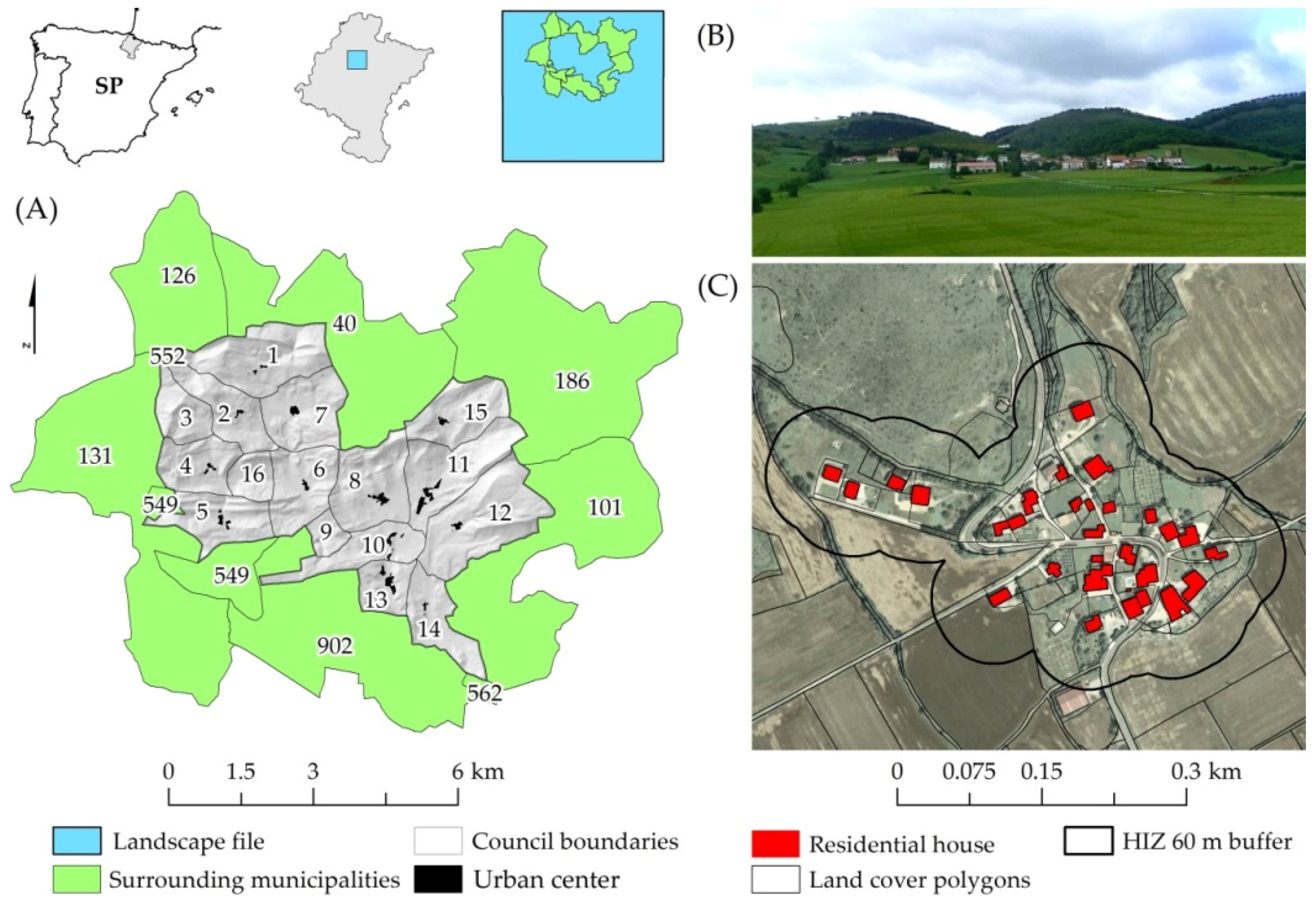
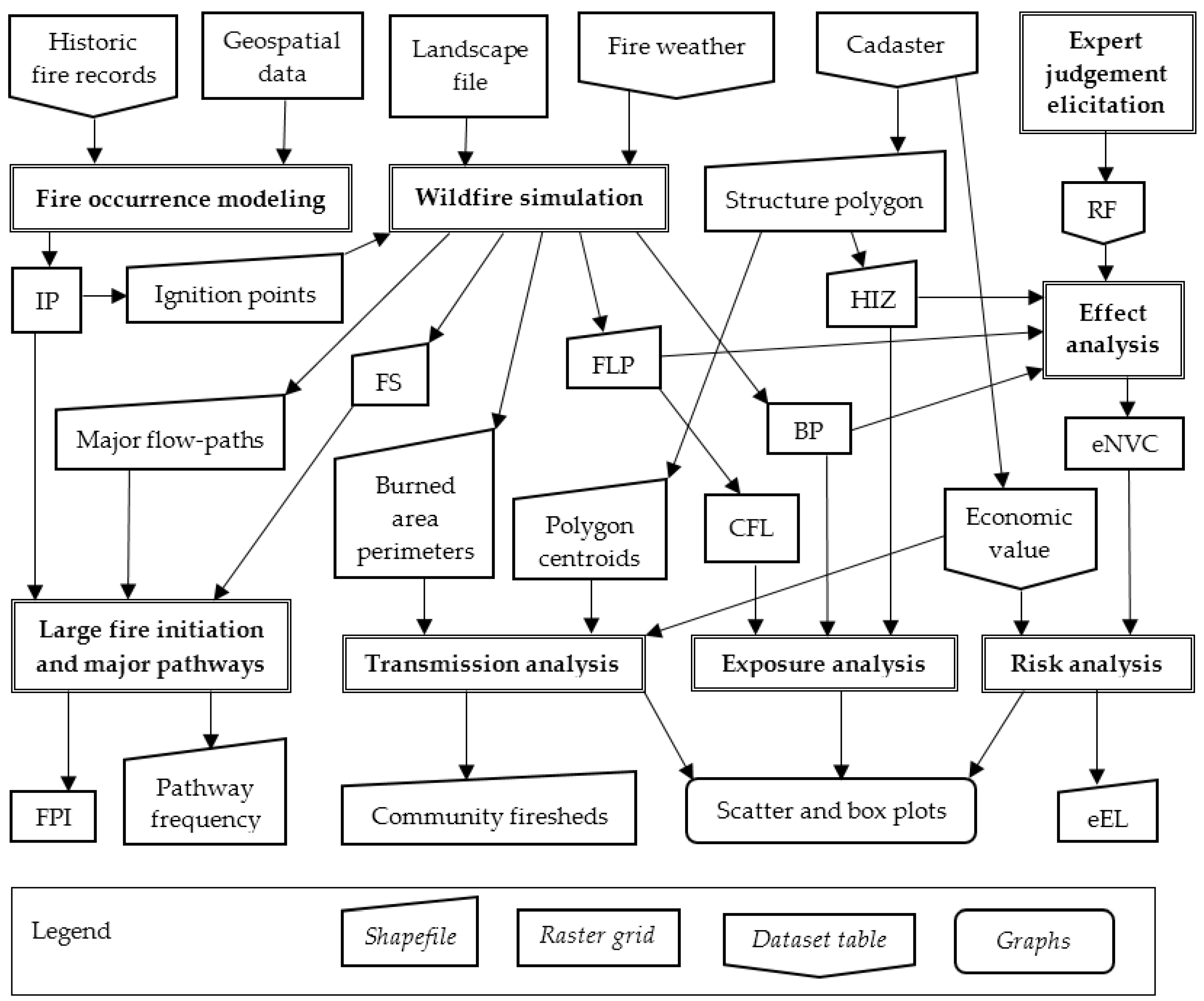
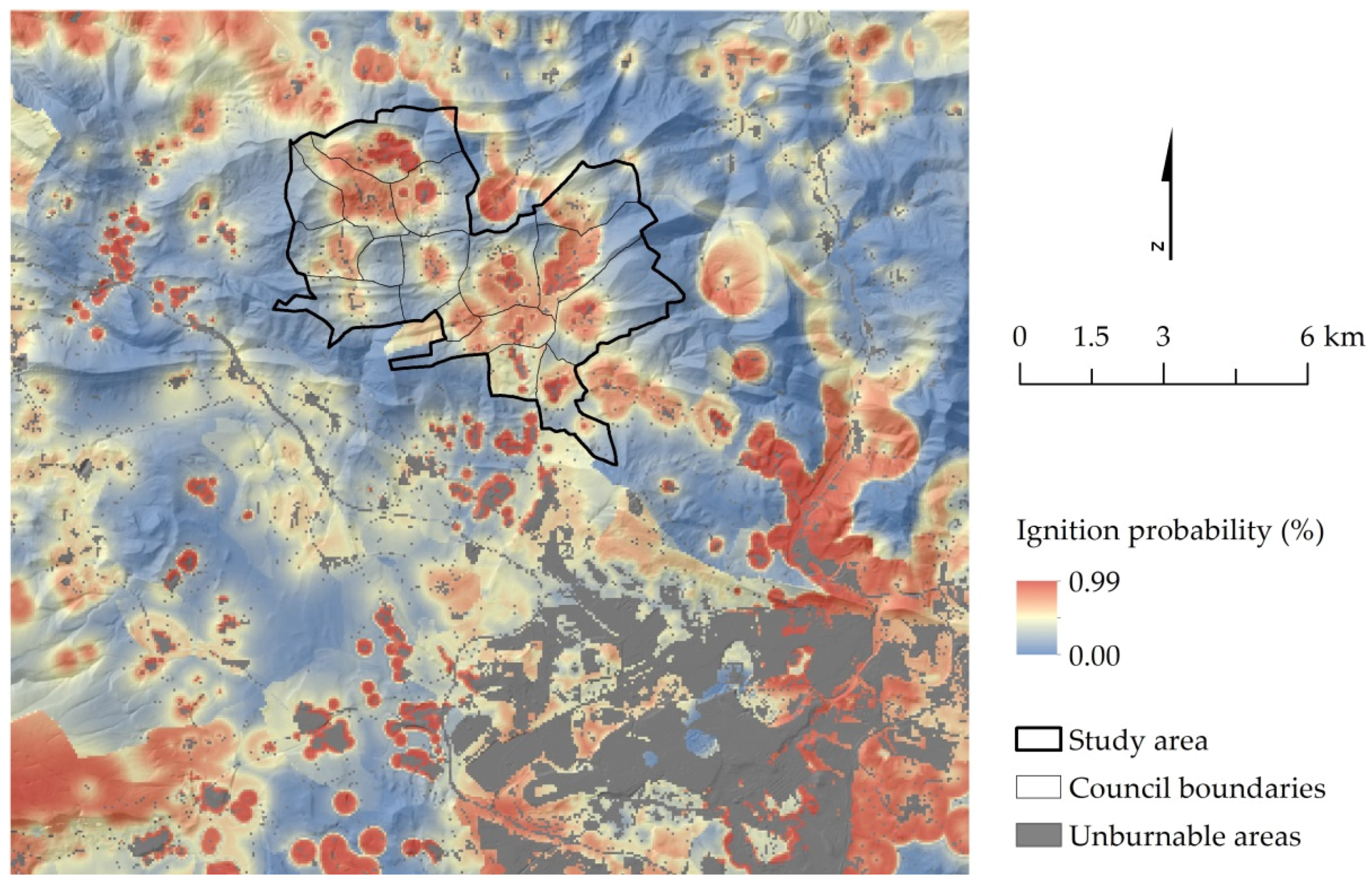
In this paper, we assess potential wildfire economic losses and transmission to residential houses in the rural communities of Juslapeña Valley, northern Spain. We used simulation modeling to map the source of wildfire exposure to communities and estimated the expected financial loss at the scale of individual structures. The simulation modeling incorporated a fine scale ignition probability grid developed from historical fire locations. Simulation outputs were used to estimate a number of exposure metrics, including burning probability and fire intensity. We estimated expected loss in the community using wildfire exposure metrics combined with a structure susceptibility function. The later was generated by a panel of local experts using an interactive structured communication technique. We also conducted a transmission analysis to delineate community firesheds and understand the source of wildfire exposure to communities. The methods provide a number of new ways to examine wildfire exposure to communities that can inform wildfire protection and improve fire resiliency in rural–urban interface areas in the Mediterranean region.

2. Material and Methods

2.1. Study Area

The study area is located in the Juslapeña Valley, central Navarra (Spain), 18 km north of the city of Pamplona (Figure 1A). The Juslapeña Valley is a 31.63 km² municipality with 548 inhabitants dispersed among 14 small rural villages or councils (minimum administrative division). The climate is transitional Mediterranean with annual rainfall around 1000 mm, a water shortage period from July to September corresponding to the wildfire season, and average maximum temperatures over 30 °C in the warmest month (meteo.navarra.es). The landscape is a mosaic of dryland cereal crops covering the valley bottom, mesoxerophytic pastures with shrubby edgings on marginal agricultural lands (Genista scorpius L., Juniperus communis L., Buxus sempervirens L., and Prunus spinosa L.), downy oak (Quercus pubescens Mill.) forests on south facing slopes (replaced by Quercus ilex L. in shallow soil foothills), beech (Fagus sylvatica L.) forests on high elevation north facing slopes, and scattered stands of black pine (Pinus nigra Arn.) [41]. Land management is largely conditioned by ownership. Most forests and natural herbaceous pastures are council common lands and agricultural fields are owned by local inhabitants. Community housing is located at mid-slopes, usually surrounded by agricultural lands and orchards at the front southern side, and forested lands arrive closer at the back (Figure 1B). We focused our analysis on residential houses (n = 306 structures), and we did not consider other structures or constructions such as agricultural warehouses. In the study area, there are no industrial sites or sport-recreational facilities. The largest observed wildfires are characterized as fast-spreading one-day summer events with less than 1000 ha burned (e.g., Juslapeña Fire in 2009 and San Cristobal Fire in 2001). Most fires are caused by humans, while lightning represents only 5% of ignitions (1985 to 2013 fire records; mapama.gob.es).

2.2. Wildfire Simulation

We gathered multiple datasets and geospatial inputs for this modeling approach (Figure 2). We simulated wildfire spread and behavior (fire size, burned area polygons, flame length probabilities, and conditional burn probability) within a 36,000-ha fire modeling domain. Overall, we conducted separated simulations for the most frequent extreme weather conditions of the wildfire season, thus obtaining different sets of modeling outputs. All the output raster grids were obtained at modeling resolution. Details are presented below in the following sections (

Table 1. Summary table with the abbreviations used in this study for the main geospatial inputs, modeling outcomes and analysis results. The terms are described and contextualized for the use in this study. We provide further details in the following sections.

Name (Abbreviation)	Description and Use
Home ignition zone (HIZ)	Area surrounding structures within a 30–60 m-buffer [11]. HIZ was used to assess wildfire exposure and risk on the individual residential houses located in the study area.
Ignition probability (IP)	Fire occurrence probability grid (0–1) generated by artificial neural network analysis [26] of historical ignition locations. It was used to calculate FPI and generate the simulated fire ignition locations.
Fire size (FS)	Fire size (ha) resulting from each individual simulated wildfire. Fire size is output from simulations along with the ignition location. It was combined with IP to generate FPI.
Fire potential index (FPI)	Is the grid generated with FS and IP, and it was used to identify large fire initiation areas [31]. The FPI provides spatially explicit valuable information to target anthropic fire ignition prevention priority areas on fire-prone landscapes.
Flame length probability (FLP)	Probability of a fire of a specific flame length given that a pixel burns under the simulated conditions. FLP is output in 0.5-m classes and sums to 1 for a given pixel. A distribution of flame lengths is generated for each pixel since fires can arrive as heading, flanking or backing fires.
Conditional flame length (CFL)	Probability-weighted flame length (m) calculated from the FLP output. CFL was summarized for the HIZ to estimate wildfire hazard and exposure to residential houses [35].
Burn probability (BP)	Number of times a pixel burns as a proportion of the total number of simulated fires (0–1). BP average values for each HIZ were used to estimate wildfire likelihood and assess wildfire exposure to residential houses [35].
Response function (RF)	The susceptibility of structures as a function of flame length represented by percent value loss (%) [42]. It was obtained from expert judgment [35].
Expected net value change (eNVC)	Expectation of gain or loss in values expressed on a percentage basis (%) [28]. Derived from combining burn probability, intensity, and susceptibility functions to estimate expected change on a percentage basis for structures [27]. Only expected losses were considered in the study.
Expected economic loss (eEL)	Expected loss expressed specifically in economic values (€) given a fire ignition and spread at assumed extreme fire weather conditions. Quantified as the product of the cadaster value of the structures and the average eNVC within the HIZ.

).

2.2.1. Landscape File and Fire Weather Input Data

We compiled the complete set of input data as required by the FlamMap fire simulator [43], including landscape file (LCP) and wildfire season extreme fire weather data. The LCP is a gridded frame containing the characteristics of the terrain, surface fuels and canopy fuel metrics. The terrain (aspect, slope and elevation) was derived from 5-m resolution digital terrain model raster data (ign.es). Standard fuel models [44,45] were assigned to 1/5000 scale land use land cover considering species composition, shrub cover and forest growth stage (idena.navarra.es and sigpac.navarra.es) (Figure 3). Canopy metrics (canopy height, canopy base height, canopy bulk density and canopy cover), were derived from low density LiDAR data (0.56 returns m²; ign.es) using FUSION [31,46]. The surface fuel and canopy metric characterization and required raster grid generation were detailed in previous studies [47,48]. The LCP was assembled at 20-m resolution [49] and comprised a 36,000-ha fire modeling domain (Figure 1A). Extreme fire weather conditions were derived using Fire Family Plus [50] from the hourly records of the Pamplona automatic weather station (1999 to 2015 records; meteo.navarra.es), as the 97th percentile ERC-G fuel moisture content [51] and wildfire season dominant winds (

Table 2. Fire weather input data, corresponding to the historical 97th percentile conditions, used for wildfire simulations. We considered the most frequent wind directions (frequency >5%) during the last 17 wildfire seasons. Historical weather data were gathered from the meteorological station of Pamplona (meteo.navarra.es). We used standard fuel models for fire modeling, see references [44,45] for further details.

Wind Scenario			Fuel Moisture Content (%)
Direction (°)	Speed (km·h−1)	Probability	Fuel Loading Category	Fuel Model [44,45]
				GS1, GR5, GR2, GR4, SH6, SH5	TU3, PCL, SH3, GR3	GR1, SH3, TL2, SH8
67.5	32	0.43	1-h	4	6	8
337.5	35	0.28	10-h	5	7	9
45.0	19	0.17	100-h	8	9	12
180.0	31	0.06	Live herbaceous	20	45	70
22.5	23	0.06	Live woody	60	85	100

GS1 = low load, dry climate grass-shrub; GR2 = low load, dry climate grass; GR4 = moderate load, dry climate grass; GR5 = low load, humid climate grass; SH6 = low load, humid climate shrub; SH5 = high load, dry climate shrub; TU3 = moderate load, humid climate timber-grass shrub; PCL = closed and low litter pine stands; SH3 = moderate load, humid climate shrub; GR3 = low load, very coarse, humid climate grass; GR1 = short, sparse dry climate grass; SH3 = Moderate load, humid climate shrub; TL2 = low load broadleaf litter; SH8 = high load, humid climate shrub.”

). We generated five wind scenarios considering the most frequent wind directions (frequency >5% in weather records) during wildfire season and the respective 97th percentile wind speeds.

2.2.2. Fire Occurrence Modeling

We used artificial neural networks (ANNs) to construct a fire occurrence model, and ultimately to generate a 20-m resolution ignition probability grid encompassing the modeling domain. A 10,000-fire ignition point input file for wildfire simulation was then created from the ignition probability (IP) grid masked to burnable fuels. ANN models are robust pattern detectors which can approximate mathematical relationships with non-normal distributions and spatially correlated variables where other statistical models could cause multicollinearity [52,53], and have been successfully applied to fire occurrence prediction in previous work [26,54].

The historical fire ignitions within the fire modeling domain (200 ignitions in all, 1985 to 2013 fire records; mapama.gob.es) and the same number of random no-fire observations were matched to topography (elevation, aspect, slope), land cover class, population density, and accessibility (distance to roads, tracks, railways, urban areas and powerlines) 20-m resolution raster grids (ign.es; idena.navarra.es). Ten percent of the fire and no-fire observation variable dataset (40 cases) was set apart for validation purposes before model building. We selected feed-forward, multilayered, non-linear, fully connected, cascade-correlation networks [55], built using Neural Works Predict^® v.3.30 software (NeuralWorks Predict® 3.30, Serial Number NPSC30-70755, Carnegie, PA, USA) [56] with an adaptive gradient learning rule, a variant of the general algorithm of back-propagation [57], and a weight decay factor which inhibited complexity of the models [58]. The historic fire records of fire and no-fire observations for model building (90%) were further divided in two. One part was used for iterative training (70%, 252 cases) and the other part (30%, 108 cases) for early stopping, the periodic assessment of performance accuracy in order to avoid losing generalization capacity due to overtraining [59]. The cascade-correlation models followed a similar procedure to [60,61], in which the model architecture (number of nodes in the hidden layer) is optimized during training.

The best model found had an 8–6–1 (input–hidden–output) structure, and classification rates of 0.78–0.73–0.69 for training–test–validation datasets (

Table 3. Classification table with the results for the best occurrence model. The model was generated with Neural Works Predict^® v.3.30 software. This occurrence model was used to generate a 20-m resolution ignition probability grid (Figure 4). Geospatial variables associated with the historical fire ignitions (200 fire ignitions, 1985 to 2013 fire records; mapama.gob.es) (1) and a random sample with the same number of no-fire observations (0) were included within the fire modeling domain. A set of 40 cases (10%) was used for the validation of the model.

Classification Rate		Class	0	1	Total
Training	0.756	0	99	32	131
	0.802	1	24	97	121
	0.779	Total	123	129	252
Test	0.679	0	36	17	53
	0.782	1	12	43	55
	0.731	Total	48	60	108
Validation	0.765	0	13	4	17
	0.609	1	9	14	23
	0.687	Total	22	18	40

). When selecting the best ANN classification model, we looked for the highest classification rate on observed and predicted fire/no-fire observations, balanced results between the three datasets and a parsimonious architecture. Variables in the model, by order of importance, were distance to forest tracks (three times input to the model), distance to urban areas (twice input to the model), distance to powerlines (twice input to the model), and population density (once input to the model). Finally, this best fire occurrence model was run at 20-m resolution pixel level to generate the ignition probability grid (IP; values ranging between 0 and 1; Figure 4).

2.2.3. Wildfire Spread and Behavior Simulation

We used FlamMap to simulate wildfires under conditions of constant fuel moisture, wind speed and wind direction [43]. We conducted five different weather scenarios at 20-m resolution, with 10,000 wildfires per scenario (Table 2). FlamMap uses the two-dimensional fire growth minimum travel time algorithm (MTT) [62], which has been widely used worldwide at a broad range of scales with multiple purposes [63,64,65,66]. The MTT algorithm replicates fire growth based on the Huygens’ principle, where the growth and behavior of the fire edge is modeled as a vector or wavefront [62], and fire spread distance is predicted by the Rothermel’s surface fire spread model [67]. Fire duration was set at 6 hour, in agreement with the active fire spread duration of the observed largest wildfire events in the study area (i.e., Juslapeña 2009). We did not consider barriers to fire spread or fire suppression efforts. Overall, modeled fires burned burnable pixels at least once and more than 100 times on average.

FlamMap outputs burn probability (BP) and flame length probability (FLP) grids, as well as a fire size (FS) text file and the fire perimeters (polygons). The burn probability (BP) is the number of times a pixel burns as a proportion of the total number of fires, and is defined as follows:

BP = F/n

(1)

where F is the number of times a pixel burns and n is the number of simulated fires per run (n = 10,000 in this study). Specifically, the conditional burn probability in the study area is the BP given that a fire ignites within the fire modeling domain and spreads for 6 hours at assumed fuel moisture and weather conditions (97th percentile fire weather). Fire intensity [68] is first predicted by the MTT algorithm [62] and is converted into flame length as:

FL = 0.0775 × I^0.46

(2)

where FL is flame length (m) and I fireline intensity (kW·m⁻¹ , kW = kilowatt). Then the program calculates a FLP regular point grid (at the fire simulation resolution) from the multiple burning fires at different flame lengths (i.e., backing, heading and flanking fire spread flame lengths). For every pixel in the FLP output, the probability of flame length is calculated at i categories of different fire intensity levels (FILs), given that at least one of the simulated fires has burned the pixel. In this study, FILs were obtained as twenty 0.5-m flame length categories (for FIL₁-FIL₁₉ and FIL₂₀ >9.5 m).

In the fire size (FS) text file output generated by FlamMap, the simulated burned area (ha) is attributed to each xy coordinate fire ignition. Moreover, we also obtained burned-area polygon shapefiles associated with each simulated fire and minimum travel time (MTT) major flow-paths polyline shapefiles for the five fire weather scenarios (Table 2). Travel pathways are straight lines that connect nodes and intersect cells to form segments for which fire behavior is calculated from the input data [43].

2.3. Expert Judgement of Structure Susceptibility

We used a response function (RF) to approximate structure susceptibility (potential losses) using fire intensity level model outputs [36]. To generate a customized RF for residential houses in the study area, we used the Delphi method [69]. The Delphi method is an iterative questionnaire process used to obtain a reliable consensus from a carefully selected expert panel, and it has been used in previous studies to determine wildfire causality from the personnel involved in fire suppression activities [70,71].

We conducted a face-to-face and anonymous two-round questionnaire process with the regional firefighting “Bomberos de Navarra” chiefs, focusing on the most experienced in WUI fire suppression in central Navarra. Fire intensity is the main causative factor of home loss given that a fire reaches a housing structure, and therefore in the questionnaire, potential value loss of structures (as a percentage) was associated to four different fire intensity class response functions (intensity levels of FIL₁, FIL₂-FIL₄, FIL₅-FIL₇, and FIL₈-FIL₂₀). The four fire intensity classes were selected considering previous studies and the capabilities of existing geospatial tools to integrate the fire modeling outputs with potential fire effects [36,49]. In the first round of the questionnaire process, the experts filled the questionnaire anonymously according to their own personal experience to reduce the effect of dominant individuals. Then in the second round, the questionnaire was repeated to the same experts, but included results from the first round (average values and deviation in the fire intensity classes) to meet a higher consensus and refine the final results. The obtained custom RF presented moderate to strong losses in housing structures as fire intensity increased (

Table 4. Custom response function (RF) used to approximate fire effects in terms of value loss (%) on residential houses in the study area [42]. The fire modeling output fire intensity levels (FILs) were grouped into four classes for the geospatial risk assessment [49]. We used the Deplhi method to obtain the susceptibility function from an expert panel composed of the most experienced firefighter chiefs on wildland urban interface fire suppression [69]. The wildfire had negative impacts in structures at all fire intensities.

Valued asset	Relative Net Value Change (%) at Different Fire Intensity Classes
	Low (FIL1)	Moderate (FIL2–FIL4)	High (FIL5–FIL7)	Very high (FIL8–FIL20)
	FL < 0.5 m	0.5 m < FL < 2 m	2 m < FL <3.5 m	FL > 3.5 m
Residential house	−10	−45	−75	−95

), similar to RFs obtained in other studies conducted in Mediterranean areas [35].

2.4. Residential House Economic Value

We used the official cadaster method described in the Navarra Foral Decree 334/2001 of November 26 to assess the economic value (V) of the individual housing structures in the study area. This Foral Decree approves the procedure for the economic assessment of immovable property in the Foral Community of Navarra throughout the implementation of the Comparison Method of the average market prices, with reference to Inheritance and Gift taxes, and over Property Transfer and Certified Legal Documents (text published in the Boletín Oficial de Navarra No. 155 of 21 December 2001, and the Boletín Oficial de Navarra No. 21 of 18 February 2002; lexnavarra.navarra.es). The method has been updated several times since its first publication, with the Foral Decree 39/2015 of 17 June being the last update. There are specific models to estimate the values for flats, single residential houses, and parking or storage rooms. We used the model for single houses, since most dwellings in the study area were well preserved rural houses or recently built constructions. The main parameters used by the model are the year of the information, type of individual house, location, cadastral category and conducted reforms, year of construction, constructed surface, and the ratio of constructed surface to urban development polygon surface. The residential houses with more than one cadastral sub-division (original building and dwelling expansion) were merged into a single unit. We used market prices from 2015 to obtain the most up-to-date values (

Table 5. Summary table of the cadaster economic value (V) for the residential houses in the Juslapeña Valley. Council polygon cadaster codes No. 3 and No. 16 do not have residential houses (Figure 1A). The cadaster value was estimated for the year 2015, considering the model published in the Foral Decree 334/2001 of November 26 (lexnavarra.navarra.es).

Cadaster (Polygon No.)	Council Name	Residential Houses (No.)	Cadaster Economic Value (€)
			Average	Median	Maximum	Minimum
1	Beorburu	11	108,825	109,767	151,432	52,124
2	Osacar	8	145,249	133,338	223,641	100,226
4	Osinaga	16	130,053	123,993	213,505	50,040
5	Aristregui	23	162,244	191,847	423,310	48,396
6	Larrayoz	17	156,733	138,493	269,403	77,480
7	Nuin	26	142,338	109,033	261,787	52,254
8	Marcalain	31	163,710	141,553	315,990	91,589
9	Iruzkun	1	132,192	132,192	132,192	132,192
10	Garciriain	12	139,194	143,079	199,405	74,682
11	Belzunce	48	168,233	135,984	483,043	64,657
12	Navaz	21	131,148	114,763	223,539	68,061
13	Ollacarizqueta	55	135,030	127,351	319,046	67,402
14	Unzu	16	154,063	174,413	218,129	88,067
15	Usi	21	111,784	108,407	167,685	71,229

).

2.5. Analysis

Wildfire simulation outputs were used to assess large fire initiation, transmission, exposure and risk to residential houses of rural communities within the study area (Figure 2). We combined five sets of fire simulation outputs (BP, FLP, FS, burned area perimeters and major flow paths), one for each scenario by weighting the relative scenario probability (Table 2).

2.5.1. Large Fire Initiation and Incoming Major Pathways

We estimated fire potential index (FPI) [31], and MTT major flow-paths to spatially analyze where large fires likely initiate and from which surrounding neighboring municipalities do these fires spread to reach the target residential houses. We calculated fire potential index (FPI) as:

FPI = FS × IP

(3)

where the FS is the spatially smoothed fire size grid, and IP is the historical-based ignition probability grid generated with the ANN fire occurrence model (Figure 4) used to generate the fire ignition input file. We used a kriging geostatistical analysis method to generate a continuous distribution grid of FS from fire size data contained in the ignition location output point file. MTT flow-paths within surrounding municipality polygons (Figure 1A) were then overlaid and classified in three frequency classes (<33%, 33%–66% and >66%), considering the simulation scenario probability (Table 2), to identify preferential pathways entering to the Juslapeña Valley.

2.5.2. Transmission Analysis

We analyzed how incoming fires are shared among surrounding municipalities (Figure 1A) and mapped the potential impact of each independent fire on dwellings with transmission analysis. We only considered large fires (>100 ha) because small fires do not substantially contribute to total burned area. In the study area observed, large fires (>100 ha) burned about 95% of the total area (1985 to 2012 historic fire records). We quantified (i) the number and (ii) the economic value of residential houses within fire perimeters. Fire transmission in terms of the number of structures was quantified as:

$$TF{S}_{ij}={\displaystyle \sum S_j}$$

(4)

where TFS measures the number of individual S affected structures in the jth municipality (study area) given a large fire (>100 ha) ignited in the ith surrounding municipality (Figure 1A) spreading under 97th percentile fire weather conditions for 6 hours. Correspondingly, the cadastral value of all affected structures contained inside the burned area from transmitted fires was quantified as:

$$TF{V}_{ij}={\displaystyle \sum V_j}$$

(5)

where TFV measures the cadaster structure value sum of all houses affected and located in j, given a fire arriving from the ith polygon, and V is the individual structure cadaster value (€). TFV is not the expected economic loss of affected structures, but the value of all affected structures within the burned area polygons. We considered j as the municipality polygon corresponding to the study area (i.e., Juslapeña Valley) containing all the target residential houses, and i as the surrounding municipality polygons (Figure 1A). In total, we analyzed the transmission of 12,515 fires larger than 100 ha ignited from the six different municipality polygons surrounding the study area. Since we focused our analysis only on fires incoming from surrounding polygons, self-burning was not considered (i.e., i ≠ j).

The TFS transmission results (i.e., the 10,000-fire ignition point file attributed with the number of structures intersected in the fire perimeter polygons) for the five different fire modeling simulation scenarios (Table 2) were separately spatialized into fireshed continuous grids using a 1000-m fixed radius and spherical semivariogram model kriging analysis statistical method. The area estimated within a fireshed is conditional on assumed fire weather and hence we estimated firesheds for each of the scenarios. We also developed contour plots using six different transmission levels to map the internal transmission gradient (0–50, 50–100, 100–150, 150–200, 200–250 and >250 structures).

2.5.3. Exposure Analysis

We analyzed individual residential house wildfire exposure in the home ignition zone (HIZ) (Figure 1C). The HIZ is the 60-m buffer immediately surrounding residential houses that determines structure ignition potential during extreme wildfire events [10]. Fire likelihood and intensity modeling outputs were considered as key causative wildfire risk factors for this analysis. Structure exposure assessment does not account for the fire effects. The geospatial location (polygons) for the individual residential house structures (n = 306) was obtained from cadaster shapefiles (1:5000 scale) of the Regional Government (catastro.navarra.es; Figure 1C).

Wildfire likelihood was estimated as conditional burn probability, and fire intensity as the conditional flame length. We used the pixel-level FIL distribution to calculate the conditional flame length (CFL) as:

$$CFL={\displaystyle \sum _{i=l}^{20}FL{P}_{\mathrm{i}}}\times F{L}_{\mathrm{i}}$$

(6)

where FLP_i is the flame length probability of a fire at the ith flame length category, and FL_i is the flame length (m) midpoint of the ith category FIL. The CFL is the probability-weighted FL assigned to a fire, and is a measure of wildfire hazard [35]. We assessed exposure at individual residential houses from the average values (BP and CFL) within the HIZ.

2.5.4. Risk Analysis

We quantified the expected losses to individual residential houses combining wildfire likelihood and intensity modeling outcomes with expert judgement elicitation response functions [28]. RFs were used to approximate fire effects (losses) to different fire intensity classes. Then, fire effects and respective burning probabilities were considered to estimate the expected net value change [36]. Expected net value change is a risk-neutral measure in terms of gain or loss expressed on a percentage basis, and allows quantitative wildfire risk assessment for multiple valued resources and human assets [33]. In order to consider the variations between economic values of different houses and quantify economic losses at the individual structure level, we used the latest cadaster reference of economic values (V).

The probabilistic expectation of loss (eNVC) was estimated by combining the customized response function with fire intensity and conditional burning probabilities [28] at the pixel-level on the HIZ:

$$eNVC={\displaystyle \sum _{i=1}^{20}BP\times FL{P}_i\times R{F}_i}$$

(7)

where eNVC is the expected net value change neutral base measure in terms of gain or loss (%) [36], BP is the conditional burn probability, FLP_i is the flame length probability of the ith category FIL, and RF_i is the response function at the ith FIL (Table 4). We assigned the average value within the HIZ to the individual dwellings.

Losses at the individual structure level were monetized using the cadaster value as:

$$eE{L}_x=eNV{C}_x\times V_x$$

(8)

where eEL is the expected economic loss in the xth residential house (€) given that a fire ignites within the wildfire modeling domain and spreads under extreme fire weather conditions, eNVC_x is the average expected net value change in the xth residential house HIZ, and V_x is the latest cadastral reference value of the xth residential house (€; catastro.navarra.es). Previously, eNVC negative values (fires always produced losses) were transformed into a positive fraction of unity value (e.g., −5% to −0.05).

3. Results

3.1. Large Fire Initiation and Major Pathways

The source location of large fires as quantified by FPI was concentrated around the southwestern and central part of the northern councils (Figure 5). Fires ignited in the south of the study area resulted in larger fire size, and therefore higher FPI values than in the northern and eastern areas. In the northwestern and eastern forested remote areas, the fire ignition probabilities were very low and consequently FPI values were the lowest compared to other areas. Incoming fires exhibited two main paths, either from the northern central part or the southeastern open valleys (Figure 3 and Figure 5). These results highlighted the effect of topography and fuel models in the major flow-paths, especially in the mountainous northern areas of the study area. Fires in the even-aged mature beech forests were largely impenetrable on the northern border within the municipality 126, and most incoming flow-paths were routed through municipality 40, where heading fire spread from the different scenarios’ pathways coincided frequently (>66%). On the other hand, in the more fire-prone unmanaged oak and black pine stands, fires arrived from south facing slopes in some cases (e.g., 180° flow-paths). Overall, herbaceous type fuel models located in lowland valley bottom flat areas facilitated the spread of fire and were the preferential fire spread pathways into the study area.

3.2. Transmission Analysis

Fires threatening the highest number of residential houses initiated in the southeast 101 and northern 40 municipalities, affecting on average 71 and 80 structures respectively (Figure 6A). The maximum number of structures affected was 188 from a fire ignited in municipality 40. Fires from municipalities 126 and 131 showed limited transmission capability with six or fewer structures burning on average. Although fires in eastern municipality 186 burned on average 15 structures, a few fires (2%) burned more than 100 structures. Due to the limited variability in cadaster economic values of structures within the study area (Table 5), both transmission boxplots depicted similar distributions (Figure 6A,B). Thus, both transmission metrics (TFS and TFV) provide equivalent results in the study area. Given the same response function for all structures (Table 4), economic losses of residential structures from large fires (>100 ha) ignited in surrounding municipalities are highly dependent on HIZ fire intensity and number of structures.

We found a wide variation in predicted community fireshed area for the different scenarios used in the fire simulation (Figure 7A–E). The southern wind direction scenario presented the largest firesheds and smooth gradients, expanding southwards more than 5 km from the study area boundary for the highest >250 structure transmission class. Fires arriving from the south burned through dryland cereal crops and represented the most extreme threat fire scenario to the residential houses in the study area (180°). Firesheds for northwestern to northeastern component wind directions presented the sharpest transitions gradients between transmission classes (337° and 67°). North facing timber litter fuel model beech stands on wind direction perpendicular orientations delineate the fireshed boundaries in northeastern and northwestern wind directions (Figure 3 and Figure 7A,D,E). Highest TFS and TFV values were obtained for fires ignited inside the study area in the majority of cases. Fireshed extension in the north was limited to valley bottom herbaceous fuels on the central part for the scenarios that present similar wind direction and mountain ridge orientation (22° to 67°). Fireshed delineation results agree with the major flow-path results, and overall on larger areas over flow-path influence areas.

3.3. Exposure Analysis

The burn probability and conditional flame length wildfire modeling outputs showed complex spatial patterns in the study area (Figure 8A,B). As expected, the results highlighted important differences between the fire occurrence IP grid (Figure 4) and conditional burn probability in structure HIZ, since fire occurrence is closely associated with anthropic ignition sources but not necessarily burn probability (Figure 9). While the average IP is usually high on the HIZ (IP >0.8), the BP presents a wide range of values between 0.001 and 0.120 (Figure 8). Southern councils presented the highest ignition probability and burn probability values (e.g., councils No. 13 and No. 14; Figure 1A). Burn probability was higher than 0.1 in most southern areas, ten times higher than values in the northern part of the study area (BP < 0.001; Figure 8A). Highest values were associated in most cases to fast spreading surface fires in herbaceous type fuel models, such as rangelands and cereal crops (the Pamplona Basin northern rim extensive dryland agricultural landscape continuum) that dominate the valley bottom in the southern plain of the study area. On the other hand, the lowest values of the northern mountainous areas corresponded to beech and pine forests on north aspects, both characterized by low biomass understories. The smooth spatial gradients in burn probability were in contrast to the conditional flame length (CFL) (Figure 8B), where CFL highest values did not correspond with high burn probability (Figure 8B and Figure 10A). Low CFL values (<1 m) were obtained in northern areas where the burn probability was the lowest, especially in the low fuel load, timber litter and closed canopy mature forest stands. Mosaics of fuel types, together with wind direction and slope, were the main drivers of fire intensity. High shrubs and dense forests on slopes aligned with the dominant winds (68° and 338° azimuth) showed the highest intensities (CFL > 6 m).

Average burn probability and conditional flame length for pixels within the 60-m circular buffer around individual residential houses varied widely among and within the different councils (Figure 10A,B). Overall, the bulk of houses had average conditional flame length values between 1.5 and 3 m, while the burn probability varied more widely, and was mostly concentrated between 0.4 and 0.11. Around some residential houses located in the central parts of the urban centers, where fuels consisted of managed gardens and orchards, the conditional flame length was the lowest (<0.25 m). Burn probability results showed much wider variations, especially between houses of different councils (Figure 10B). For instance, the residential houses in council No. 15 (located in the northeast, Figure 1A) presented on average four to five times lower burn probability (BP~0.02) compared to the most meridional council No. 13 (BP~0.10). Within the same urban center, residential houses exhibited variations among southern and northern locations, especially in the central parts of the study area (e.g., councils No. 5, No. 6 and No. 8), mainly because upslope spreading fires over cereal crops on the southern sides of urban centers present the fastest spread rates. Therefore, housing aggregation into compact urban centers and the relative structure position in the urban center had a strong effect on HIZ wildfire likelihood. In other words, wildfires were more likely to arrive and impact the southern side, and structures located there were exposed to higher BP. The highest overall exposure was experienced by residential houses nestled within forested and shrubby unmanaged areas with high fuel accumulation.

3.4. Expected Economic Loss

Expected economic loss for individual dwellings (eEL) ranged from a low of 740 to a high of 28,725€ within the study area (mean = 7955€), and also varied widely among the different councils (Figure 11,

Table 6. Council level summary table with expected economic loss (eEL) results for the residential houses in the Juslapeña Valley (Figure 1A). Potential expected economic loss was obtained as a result of the implementation of the framework presented in this study (Figure 2). Council polygon cadaster codes No. 3 and No. 16 do not have residential houses (Figure 1A).

Cadaster (Polygon No.)	Council Name	Residential Houses (No.)	Expected Economic Loss (€)
			Average	Median	Maximum	Minimum
1	Beorburu	11	2803	2826	4248	1120
2	Osacar	8	6378	6263	10,004	3776
4	Osinaga	16	7343	7188	12,459	2870
5	Aristregui	23	12,976	12,480	28,086	3051
6	Larrayoz	17	8347	8152	16,049	1062
7	Nuin	26	5930	4855	11,757	2425
8	Marcalain	31	8167	7502	17,855	1334
9	Iruzkun	1	9592	9592	9707	9478
10	Garciriain	12	9715	9443	14,366	5169
11	Belzunce	48	8044	6232	28,725	2143
12	Navaz	21	6157	5341	9909	3150
13	Ollacarizqueta	55	9105	8219	21,046	3960
14	Unzu	16	13,323	13,419	24,757	6933
15	Usi	21	1429	1222	3131	740

). The highest average values were obtained for the southern council No. 14 with 13,323€, followed by councils No. 5 and No. 10 with 12,976€ and 9715€ respectively. On the other hand, the lowest average eEL values were obtained in the low wildfire exposure northern councils No. 1 and No. 15, with 1429€ and 2803€ respectively. Overall, results depicted higher expected economic loss (eEL) for residential houses presenting lower expected net value change (eNVC), that ranged from −1.04% to −11.04%, with an average value of −5.23%. Except for a few cases, most residential houses have cadastral values between 110 and 180 thousand euros (Table 5), and therefore exposure metrics required for risk assessment translated similar patterns into risk outcomes (i.e., higher losses for higher overall exposure). Nonetheless, when the cadastral value varied substantially for the same eNVC (e.g., more than three times), wide differences were observed in terms of eEL. In those cases, the residential house cadastral value influenced the eEL result more than the eNVC (Figure 11).

The map of eEL for dwellings in the study area showed how spatial location greatly influenced the result (Figure 12A). Highest economic losses (>10,000€) were located in the southern councils (i.e., No. 14, No. 5 and No. 13) and some individual houses in councils of the central part, while the lowest values (<1000€) were concentrated in the northeastern and northern councils (i.e., No. 1 and No. 15). The highest variation within residential houses of the same council were seen when the urban center tended to present a more scattered linear orientation following the communication corridors (e.g., council No. 11), and greater distances between the most distant houses (>1 km). Spatial patterns in eEL were similar to the gradient observed for the burn probability (Figure 8A), since fire hazard among residential houses (Figure 10A,B) within the study area did not show large differences. Thus, according to the results at individual residential structure level, eEL treatment priorities in the HIZ would be preferentially located in southern councils and structures occluded in hazardous forest fuels.

4. Discussion

The integration of biophysical fire modeling with susceptibility relationships derived from expert judgement provides a method to calculate expected financial loss to communities from potential wildfire events. Our analysis also demonstrated the tracking of burned areas in the communities to ignition locations, thus providing a linkage between wildland fuels and risk to communities. The results provided useful insights that can inform ignition prevention fuel management programs for reducing risk to communities [72]. 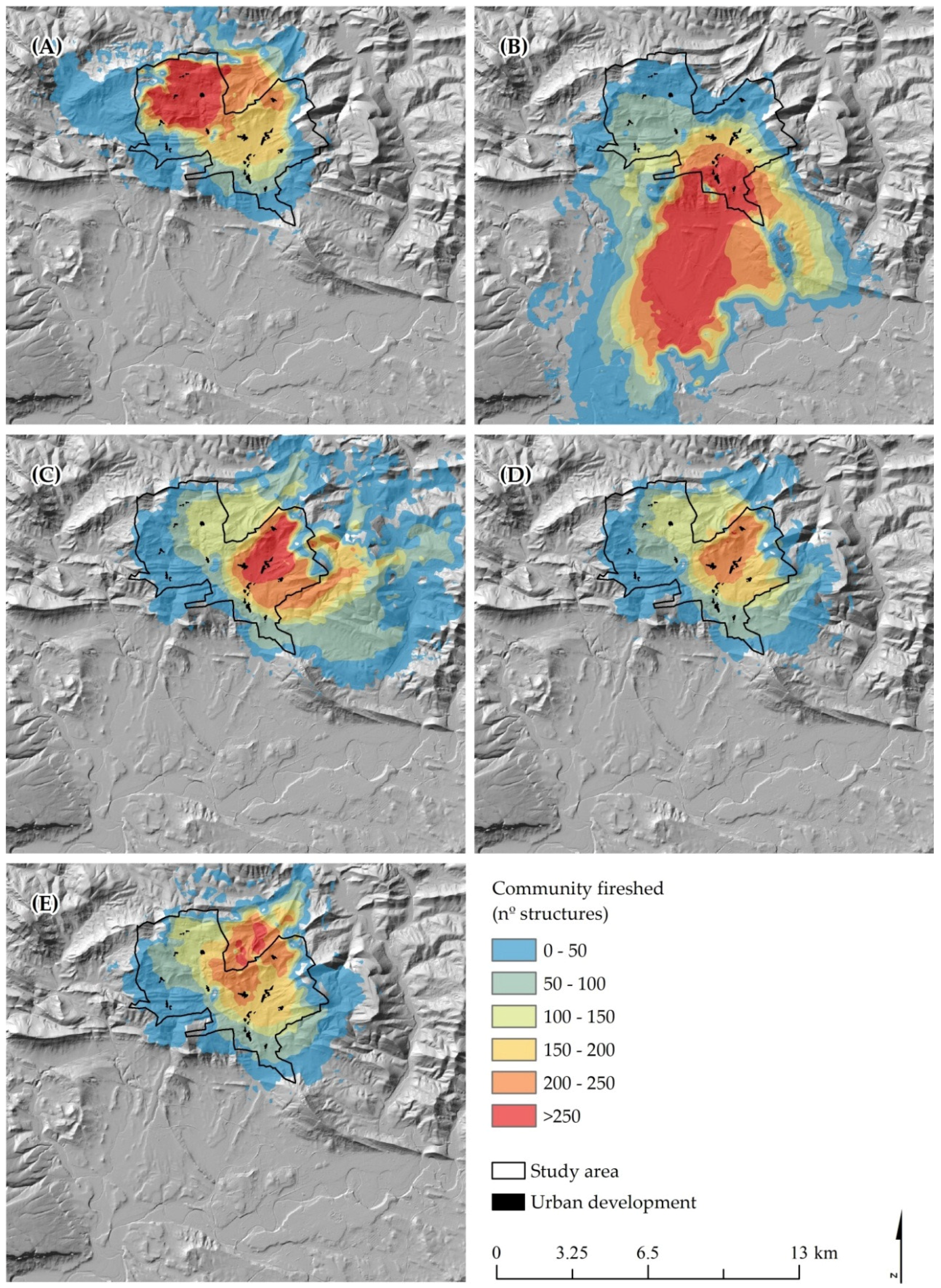Transmission analysis allows the identification of sources of risk in terms of specific landowners within the study area [39,40]. The fireshed mapping defined the scale of risk to rural communities [73] and delineated the area within which fuel treatments could be prioritized to reduce large-fire impacts [37]. 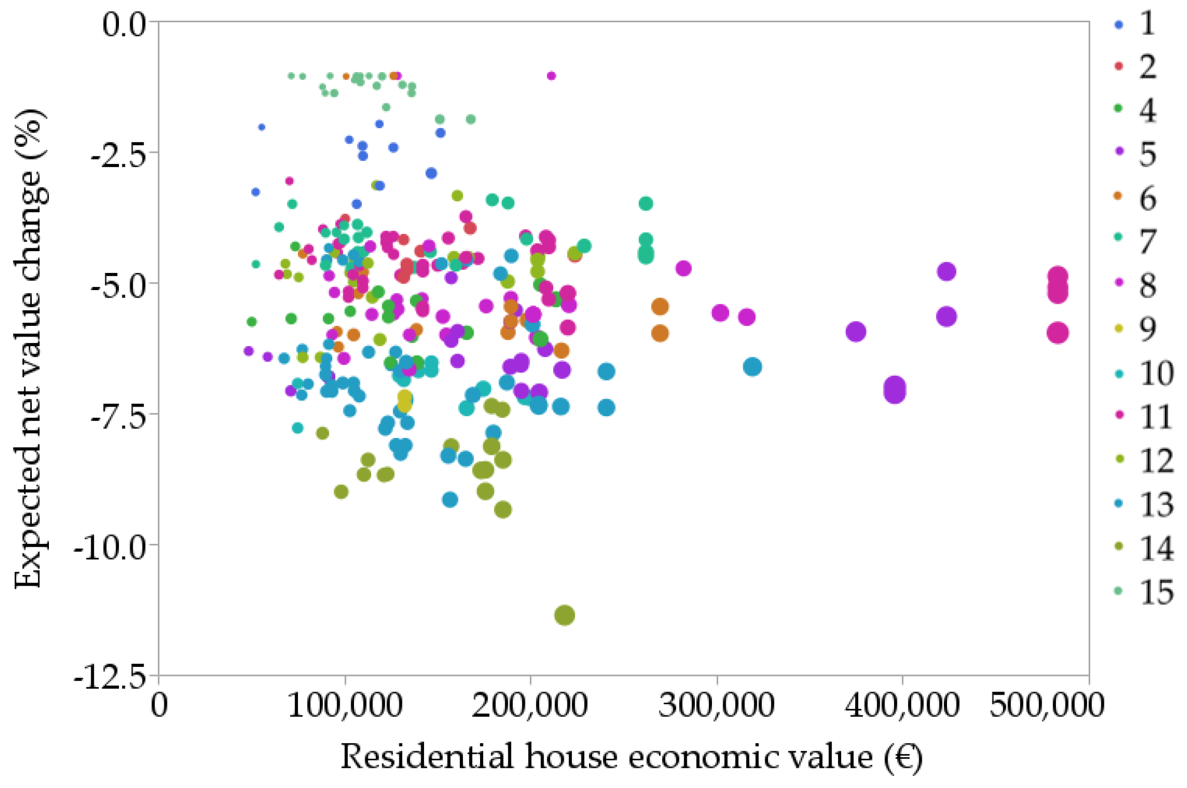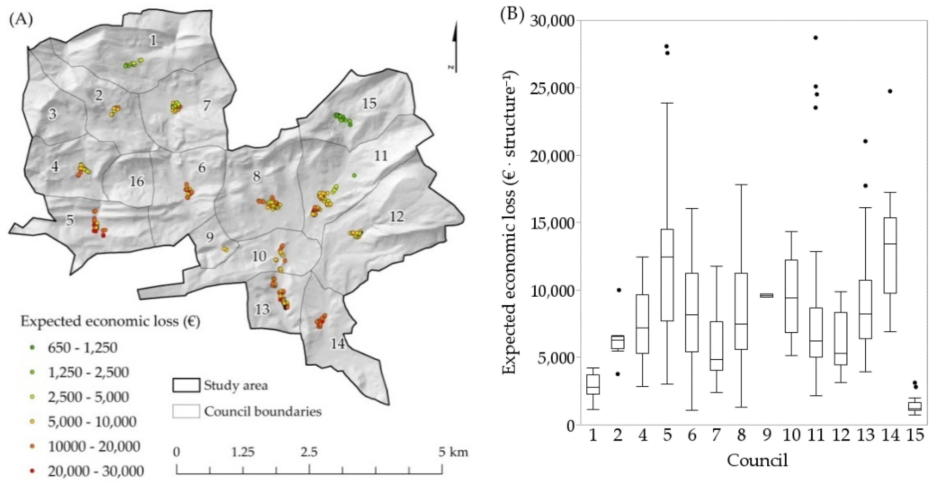Coupling the fireshed with maps of exposure provides a wealth of information to inform the prioritization of wildfire management within the study area [35]. Our fire risk quantitative assessment results showed a very strong structure-level spatial gradient in economic loss within and among the 14 councils in the Juslapeña Valley study area, and provided findings that are potentially useful for insurance companies and local landscape managers.

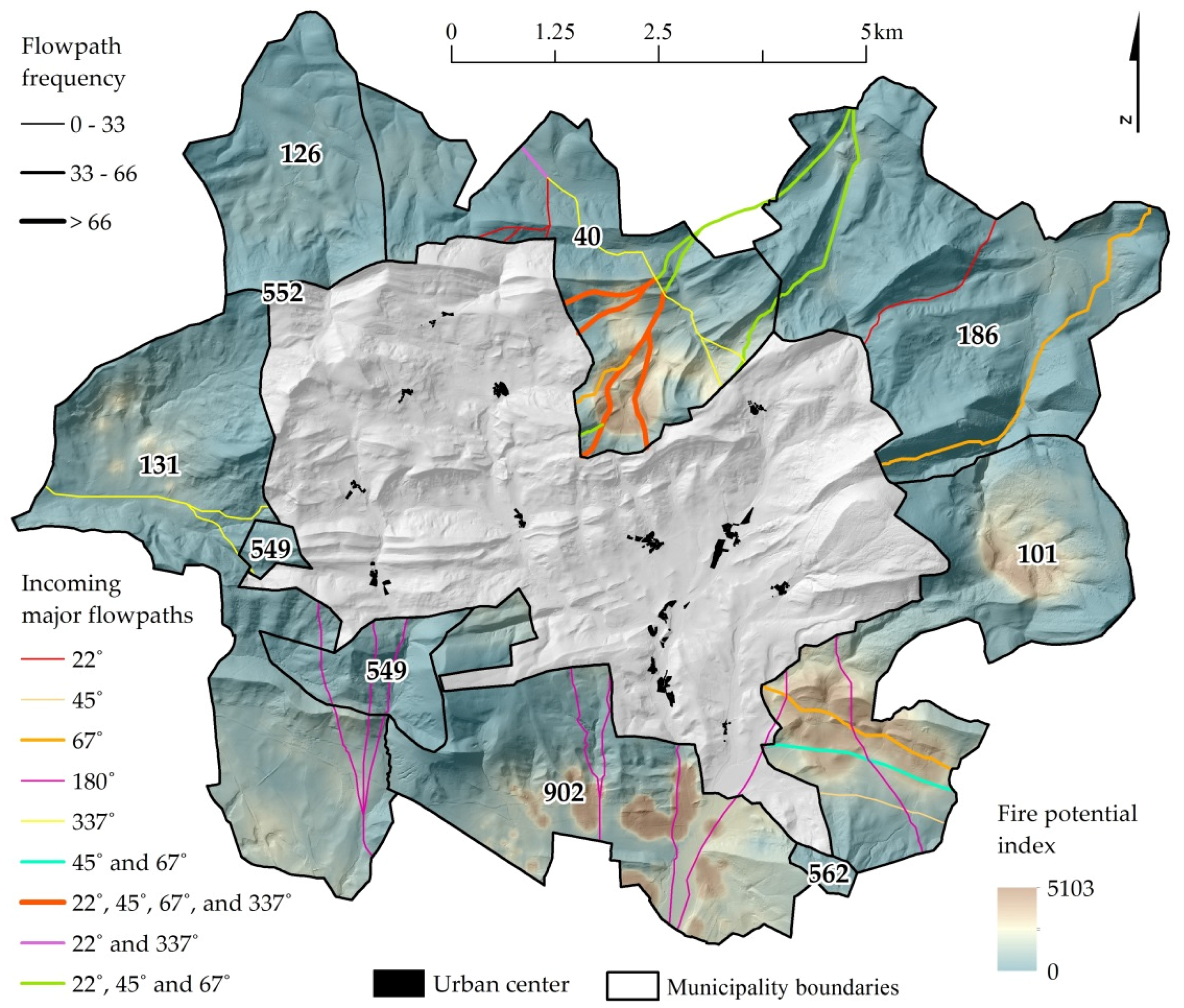
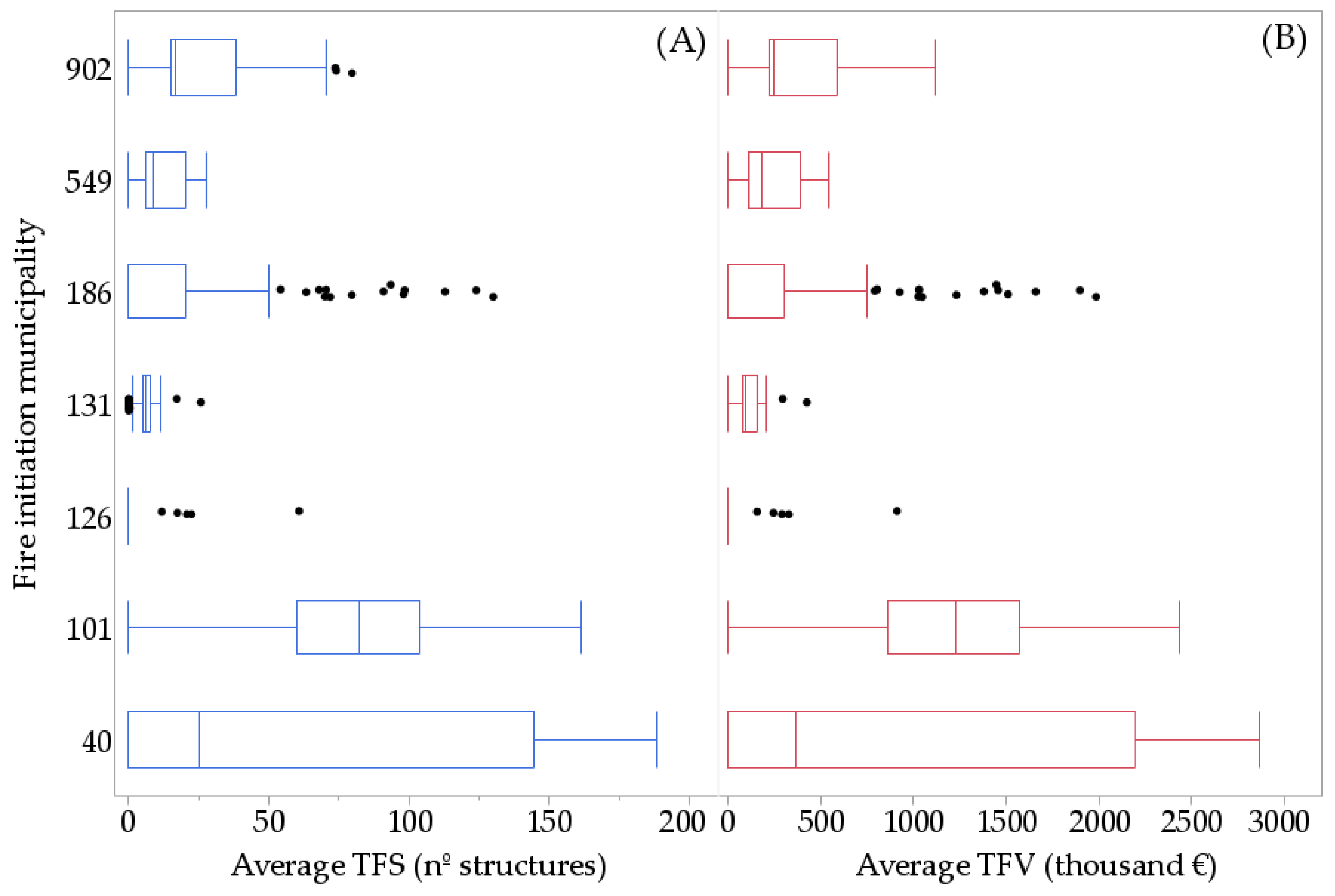
We identified high probability paths of incoming fire in central north and south east valley bottom flat areas [62,65], which were mainly located in neighboring municipalities 101 and 40. These two areas accounted for the bulk of the transmission as measured by the highest number of residential structures affected. Historically, fires frequently have impacted populated areas after spreading large distances from their ignition location, well beyond community wildfire planning boundaries, underscoring the importance of analyzing firesheds to minimize scale mismatches [41] between the landscape planning and fire risk mitigation efforts [73]. In fact, 67% of large fires (>100 ha) ignited in the surrounding municipalities reached target communities, and each of these fires affected 56 structures on average. Also, we found that the 180° wind direction fire weather scenario in particular resulted in fires spreading the longest distance from ignitions outside the study area administrative boundary (>8 km). Thus, collaborative planning efforts need to involve neighboring administrations and landowners (Figure 7), and the significance of current land management in areas outside of target councils needs to be recognized for its potential to enhance wildfire risk. These practices include grazing, firewood collection in coppice oak forests and thinning in dense conifer plantations.

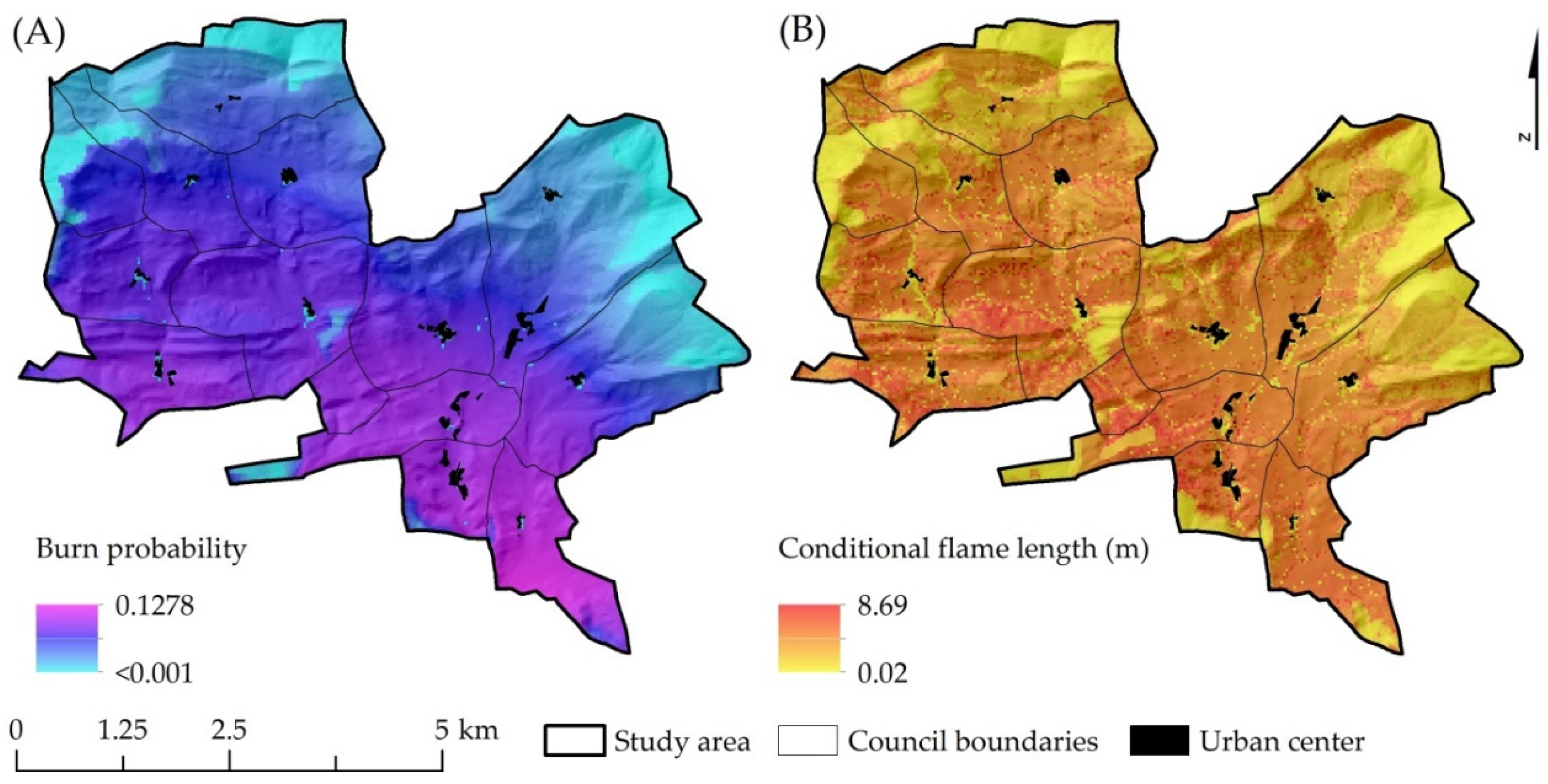
We contribute several new methods for exposure assessments within the Mediterranean region [47,72]. In particular, we used an ANN fire occurrence model to generate fire ignition input locations, and included an expert-defined response function for structure-scale assessment of potential economic losses. Although wildfire loss or benefit quantification is not possible for many socioeconomic values, a number of important services derived from forests can be represented with market pricing [48]. Specifically, 72% of structures have estimated values ranging from 100 to 250 thousand euros, with relatively few (6%) having values >250 thousand euros. Rather than economic value, we found that spatial patterns of wildfire likelihood were the major causative risk factor, and thus fire occurrence spatiotemporal patterns in Mediterranean environments are especially important for fire prevention. ANN performed well and facilitated the generation of a high-resolution ignition probability grid. Understanding how fire weather and geospatial variables associated with anthropic activities can explain fire occurrence has been conducted in previous works [74,75].

This study highlighted the importance of fire spread modeling for risk assessment in Mediterranean environments where large fires spread through mosaics of fuel type and administrative jurisdiction [32,76,77]. Urban interface classification based on housing density has been considered a key factor in structure loss and risk mitigation in some previous studies [19,78]. 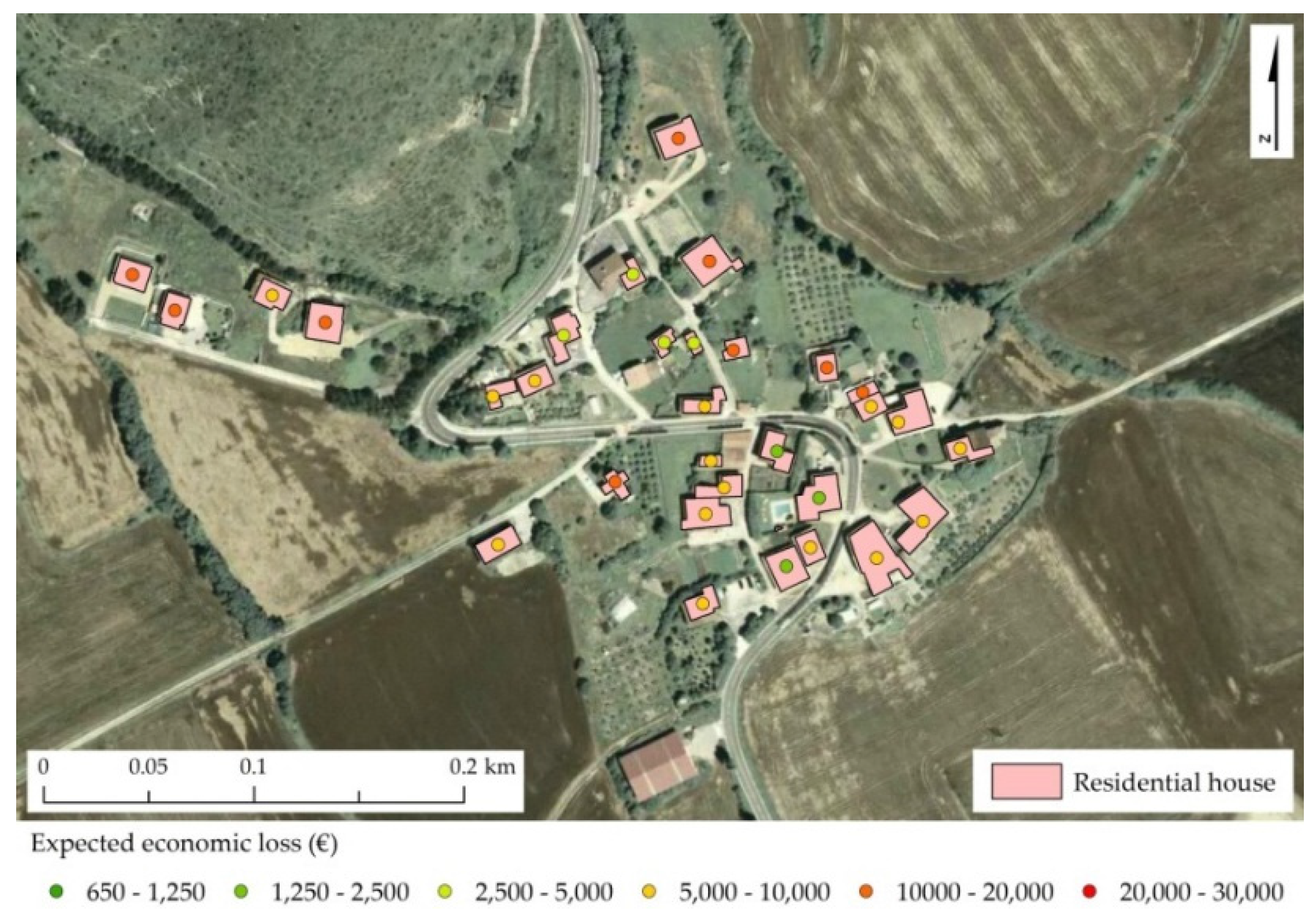Indeed, scattered and occluded houses within wildlands usually present higher exposure levels from catastrophic fire events than densely populated urban development areas [79]. However, structures at the periphery of communities usually incur higher losses since they intercept heading fires and associated embers showers (Figure 13). Although most houses in the study area are built with fire-resistant designs and materials, and have cultivated orchards in the surroundings, exposure to ember showers makes them vulnerable to fire. Isolated dwellings in remote areas are hampered by poor access for ground-based suppression crews, a primary factor contributing to structure loss probability and human fatalities [34]. Urban areas with fire-resistant structures and managed fuels in the HIZ can facilitate fire suppression opportunity, and help relocate residents to save zones during catastrophic fires events. The more typical situation is where developed areas become a resource sink for most of the firefighting resources, creating the potential for entrapment and accidents during mass evacuation during extreme fire events [80].

Multiple management implications result from this study. First, the results provided useful insights to identify preferential areas for future urban development (e.g., high overall exposure area exclusion criteria) and to inform fire-resistant building design and material requirements. Integrating exposure from other natural hazards such as floods in river basin plains and rock falls or avalanches in mountainous areas is widely accepted as criteria for potential urban development, but fire risk is not accounted in most fire prone areas where catastrophic fires are frequent events (<30 years). In this regard, many southern EU governments concerned with WUI problems are now dictating specific public policies and municipal ordinances to promote community and homeowner involvement in hazardous fuel management. We present structure level risk assessment results that can contribute to risk reduction efforts by identifying where fuel treatment provides the highest benefits at the individual house level. Urban planning and fire managers have limited budgets to cover risk mitigation over thousands of scattered housing communities dispersed throughout fire prone landscapes, and quantitative risk assessment frameworks [28,33,66] can help prioritize planning and investments as well help design specific spatial strategies [81,82].

Reducing structure susceptibility to fire [34] in combination with fuel treatments, both in HIZ [83] and strategically located areas on the landscape [10,35], are the key to mitigating wildfire risk to communities. Fuel treatments reduce potential fire intensity and spread rates by reducing surface and canopy fuel loadings and include a wide range of activities (prescribed burns, low pruning and low fuel load hedges, disrupting tree crown continuity and removing combustible material adjacent to structures) [12,84,85]. Other measures such as the implementation of structure self-protection plans can alleviate extreme fire environments and improve suppression capabilities (e.g., water sprinklers and cannons). Apart from typical treatments in forest fuels and reducing structure susceptibility, other strategies that focus on reducing fire spread over herbaceous land cover could reduce the impacts of long-distance spreading fire events. For instance, we observed long-distance fire events originating in dryland croplands in the southern portion of the study area. By managing herbaceous fuels with extensive grazing in fenced pasture common lands [86,87], and using grass species with patchy growth habit on dryland hay meadows, wildfire spread and intensity could be reduced in these areas. However, implementation of supervised grazing after cereal harvesting that is needed to break fuel beds on the edges between mosaics of cultivated lands is nowadays complicated to implement [88]. Currently, the major risk mitigation effort in agricultural areas is the prevention of ignitions during cereal harvesting operations from equipment, and increasing capabilities for more rapid response to ignitions if they do happen [89].

We assume various sources of error in the models and input data, and results should be viewed as a local approximation of wildfire risk to residential houses in Juslapeña Valley given a large fire event in the study area. Modeling outcomes are conditioned to a specific configuration of extreme fire weather conditions, fuels, topography and the rural–urban interface spatial distribution of the study area. Although fuel models around structures did not differ much from the dominant types in the study area, elsewhere complex interface areas with trimming hedges among structures (e.g., cypress Cupressus sempervirens L. hedges) might require a more detailed fuel characterization or various different response functions depending on secondary variables in addition to fire intensity. Community firesheds should be interpreted as a dynamic boundary that changes with assumptions about fire weather, and with existing spatial patterns of fuels as influenced by land management practices. The latter includes forest management practices, grazing practices and agricultural production. Moreover, structure loss is a complex process [12], and is difficult to model at the landscape scale [35]. As in other previous studies, we adopted an expert-defined response function to approximate fire effects at different fire intensities while acknowledging the margin of error [36]. We also did not consider the potential effects of fire suppression that could affect our estimates of structure ignition, especially for low intensity fires with flame lengths <1.2 m [90]. We also understand that structure economic value (conditioned to market changes) might not always be the best way to quantify real risk, due to the lack of correlation among the economic value and the social impact of structure loss on inhabitants. Focusing exclusively on economic criteria when setting treatment priorities might bias results to favor protection of the wealthy neighborhoods at the expense of lower priced homes, although in our study the value of homes did not substantially influence the results.

Further research is needed to better understand not only large fire transmission into the study area, but also the dominant transmission patterns at wider scales (e.g., regional and national), to understand how the study area is integrated into larger scale fire transmission patterns [40]. Understanding major large fire movements would provide a wider perspective to identify the nodes or high priority areas in the landscape requiring investments in treatments. Identification of treatment polygons or stands in priority areas (or firesheds) can be facilitated with optimization models and trade-off analysis to maximize the reduction in risk to multiple values of interest, including structure loss, game species habitat improvement or conifer timber production [91]. The risk assessment in this study should be considered as a preliminary step for mitigation and it does not necessarily reveal the optimal treatment allocation, especially considering that treating fuels at locations far from the urban interface can substantially slow large fire arrival [35]. Analyzing multi-objective treatment strategies in rural–urban intermix fire-prone Mediterranean EU landscapes is challenging, although newer landscape planning tools that allow for integration of fire transmission have opened a wide range of new analytical approaches to analyze trade-offs between local hazard versus large-scale transmitted fire [81].

5. Conclusions

We implemented a fine scale wildfire risk assessment and transmission framework in rural communities of central Navarra (Northern Spain). Potential economic losses were quantified on individual residential houses considering exposure results [42], local expert-defined susceptibility functions, and dwellings cadaster economic values. With the transmission analysis we traced the origin and quantified the potential impacts of large wildfires [40]. Using major flow-paths [62] we identified preferential fire spreading path-ways entering to the study area. We demonstrate that wildfires ignited in neighboring municipalities far beyond human communities can cause substantial economic losses. This work increases the awareness and knowledge on wildfire risk assessment in Southern European fire-prone areas, and highlights the need of a collaborative planning and management among neighboring communities, different landowners and landscape managers to mitigate losses from wildfires.

References

1. Radeloff, V.C.; Hammer, R.B.; Stewart, S.I.; Fried, J.S.; Holcomb, S.S.; McKeefry, J.F. The wildland-urban interface in the United States. Ecol. Appl. 2005, 15, 799–805. [Google Scholar] [CrossRef]
2. Price, O.; Bradstock, R. Landscape scale influences of forest area and housing density on house loss in the 2009 Victorian bushfires. PLoS ONE 2013, 8, e73421. [Google Scholar] [CrossRef] [PubMed]
3. Martinuzzi, S.; Stewart, S.I.; Helmers, D.P.; Mockrin, M.H.; Hammer, R.B.; Radeloff, V.C. The 2010 Wildland-Urban Interface of the Conterminous United States—Geospatial Data; Service U.F.: Fort Collins, CO, USA, 2015. [Google Scholar]
4. Maillé, E.; Fernández, M.M.; Bouillon, C.; Sirca, C. Wild Fire Risk in the Rural-Urban Interface. In Forest Fires under Climate, Social and Economic Changes in Europe, the Mediterranean and Other Fire-Affected Areas of the World-Fume-Lessons Learned and Outlook; Arianoutsou, M., González-Cabán, A., Mouillot, F., Oechel, W.C., Spano, D., Thonicke, K., Vallejo, V.R., Vélez, R., Eds.; Calyptra Pty Ltd.: Adelaide, Australia, 2014; pp. 14–15. [Google Scholar]
5. Bouillon, C.; Fernandez Ramiro, M.M.; Sirca, C.; Fierro Garcia, B.; Casula, F.; Vila, B.; Long Fournel, M.; Pellizzaro, G.; Arca, B.; Tedim, F.; et al. A Tool for Mapping Rural-Urban Interfaces on Different Scales. In Advances in Forest Fire Research; Viegas, Domingos Xavier: Coimbra, Portugal, 2014; pp. 611–625. [Google Scholar]
6. Pausas, J.G. Simulating mediterranean landscape pattern and vegetation dynamics under different fire regimes. Plant Ecol. 2006, 187, 249–259. [Google Scholar] [CrossRef]
7. Theobald, D.M.; Romme, W.H. Expansion of the US wildland–urban interface. Landsc. Urban Plan. 2007, 83, 340–354. [Google Scholar] [CrossRef]
8. Badia, A.; Serra, P.; Modugno, S. Identifying dynamics of fire ignition probabilities in two representative mediterranean wildland-urban interface areas. Appl. Geogr. 2011, 31, 930–940. [Google Scholar] [CrossRef]
9. Pellizzaro, G.; Arca, B.; Pintus, G.; Ferrara, R.; Duce, P. Wildland Urban Interface Dynamics during the Last 50 Years in North East SARDINIA. In Modelling Fire Behavior and Risk; Spano, D., Bacciu, V., Salis, M., Sirca, C., Eds.; Nuova Stampa Color Publishers: Muros, Spain, 2012; pp. 249–254. [Google Scholar]
10. Costa, P.; Castellnou, M.; Larrañaga, A.; Miralles, M.; Daniel, K. Prevention of Large Wildfires Using the Fire Types Concept; Cerdanyola del Vallès: Barcelona, Spain, 2011. [Google Scholar]
11. Cohen, J. The wildland-urban interface fire problem: A consequence of the fire exclusion paradigm. For. History Today 2008, 3, 20–26. [Google Scholar]
12. Mell, W.E.; Manzello, S.L.; Maranghides, A.; Butry, D.; Rehm, D.B. The wildland-urban interface fire problem: Current approaches and research needs. Int. J. Wildland Fire 2010, 19, 238–251. [Google Scholar] [CrossRef]
13. Moritz, M.A.; Batllori, E.; Bradstock, R.A.; Gill, A.M.; Handmer, J.; Hessburg, P.F.; Leonard, J.; McCaffrey, S.; Odion, D.C.; Schoennagel, T.; et al. Learning to coexist with wildfire. Nature 2014, 515, 58–66. [Google Scholar] [CrossRef] [PubMed]
14. USDA-USDI (2014). The National Strategy: The Final Phase in the Development of the National Cohesive Wildland Fire Management Strategy; United States Department of Agriculture: Washington, DC, USA, 2014; p. 93.
15. Calviño-Cancela, M.; has-Amil, M.L.; García-Martínez, E.D.; Touza, J. Wildfire risk associated with different vegetation types within and outside wildland-urban interfaces. For. Ecol. Manag. 2016, 372, 1–9. [Google Scholar] [CrossRef]
16. Gibbons, P.; Van Bommel, L.; Gill, A.M.; Cary, G.J.; Driscoll, D.A.; Bradstock, R.A.; Knight, E.; Moritz, M.A.; Stephens, S.L.; Lindenmayer, D.B. Land management practices associated with house loss in wildfires. PLoS ONE 2012, 7, e29212. [Google Scholar] [CrossRef] [PubMed]
17. Madrigal, J.; Ruiz, J.A.; Planelles, R.; Hernando, C. Characterization of wildland-urban interfaces for fire prevention in the province of Valencia (Spain). For. Syst. 2013, 22, 249. [Google Scholar] [CrossRef]
18. Lampin-Maillet, C.; Jappiot, M.; Long, M.; Christophe, B.; Morge, D.; Ferrier, J.P. Mapping wildland-urban interfaces at large scales integrating housing density and vegetation aggregation for fire prevention in the South of France. J. Environ. Manag. 2010, 91, 732–741. [Google Scholar] [CrossRef] [PubMed] [Green Version]
19. Herrero-Corral, G.; Jappiot, M.; Bouillon, C.; Long-Fournel, M. Application of a geographical assessment method for the characterization of wildland-urban interfaces in the context of wildfire prevention: A case study in Western Madrid. Appl. Geogr. 2012, 35, 60–70. [Google Scholar] [CrossRef]
20. Conedera, M.; Tonini, M.; Oleggini, L.; Orozco, C.V.; Leuenberger, M.; Pezzatti, G.B. Geospatial approach for defining the wildland-urban interface in the alpine environment. Comput. Environ. Urban Syst. 2015, 52, 10–20. [Google Scholar] [CrossRef]
21. Chuvieco, E.; Aguado, I.; Jurdao, S.; Pettinari, M.L.; Yebra, M.; Salas, J.; Hantson, S.; de la Riva, J.; Ibarra, P.; Rodrigues, M.; et al. Integrating geospatial information into fire risk assessment. Int. J. Wildland Fire 2014, 23, 606. [Google Scholar] [CrossRef]
22. Ganteaume, A.; Jappiot, M. What causes large fires in Southern France. For. Ecol. Manag. 2013, 294, 76–85. [Google Scholar] [CrossRef]
23. Curt, T.; Fréjaville, T.; Lahaye, S. Modelling the spatial patterns of ignition causes and fire regime features in Southern France: Implications for fire prevention policy. Int. J. Wildland Fire 2016, 25, 785–796. [Google Scholar] [CrossRef]
24. Salis, M.; Ager, A.A.; Alcasena, F.J.; Arca, B.; Finney, M.A.; Pellizzaro, G.; Spano, D. Analyzing seasonal patterns of wildfire exposure factors in Sardinia, Italy. Environ. Monit. Assess. 2015, 187, 1–20. [Google Scholar] [CrossRef] [PubMed]
25. Mann, M.L.; Batllori, E.; Moritz, M.A.; Waller, E.K.; Berck, P.; Flint, A.L.; Flint, L.E.; Dolfi, E. Incorporating anthropogenic influences into fire probability models: Effects of human activity and climate change on fire activity in California. PLoS ONE 2016, 11, e0153589. [Google Scholar] [CrossRef] [PubMed]
26. Miller, C.; Ager, A.A. A review of recent advances in risk analysis for wildfire management. Int. J. Wildland Fire 2013, 22, 1–14. [Google Scholar] [CrossRef]
27. Finney, M.A. The challenge of quantitative risk analysis for wildland fire. For. Ecol. Manag. 2005, 211, 97–108. [Google Scholar] [CrossRef]
28. Bar Massada, A.; Radeloff, V.C.; Stewart, S.I.; Hawbaker, T.J. Wildfire risk in the wildland–urban interface: A simulation study in Northwestern Wisconsin. For. Ecol. Manag. 2009, 258, 1990–1999. [Google Scholar] [CrossRef]
29. Haas, J.R.; Calkin, D.E.; Thompson, M.P. A national approach for integrating wildfire simulation modeling into wildland urban interface risk assessments within the United States. Landsc. Urban Plan. 2013, 119, 44–53. [Google Scholar] [CrossRef]
30. Salis, M.; Ager, A.; Arca, B.; Finney, M.A.; Bacciu, V.; Duce, P.; Spano, D. Assessing exposure of human and ecological values to wildfire in Sardinia, Italy. Int. J. Wildland Fire 2013, 22, 549–565. [Google Scholar] [CrossRef]
31. Alcasena, F.J.; Salis, M.; Vega-García, C. A fire modeling approach to assess wildfire exposure of valued resources in Central Navarra, Spain. Eur. J. For. Res. 2015, 135, 87–107. [Google Scholar] [CrossRef]
32. Calkin, D.C.; Finney, M.A.; Ager, A.A.; Thompson, M.P.; Gebert, K.G. Progress towards and barriers to implementation of a risk framework for us federal wildland fire policy and decision making. For. Policy Econ. 2011, 13, 378–389. [Google Scholar] [CrossRef]
33. Penman, T.D.; Nicholson, A.E.; Bradstock, R.A.; Collins, L.; Penman, S.H.; Price, O.F. Reducing the risk of house loss due to wildfires. Environ. Model. Softw. 2015, 67, 12–25. [Google Scholar] [CrossRef]
34. Mitsopoulos, I.; Mallinis, G.; Arianoutsou, M. Wildfire risk assessment in a typical Mediterranean wildland–urban interface of Greece. Environ. Manag. 2014, 55, 900–915. [Google Scholar] [CrossRef] [PubMed]
35. Thompson, M.P.; Calkin, D.E.; Gilbertson-Day, J.W.; Ager, A.A. Advancing effects analysis for integrated, large-scale wildfire risk assessment. Environ. Monit. Assess. 2011, 179, 217–239. [Google Scholar] [CrossRef] [PubMed]
36. Ager, A.A.; Day, M.A.; Finney, M.A.; Vance-Borland, K.; Vaillant, N.M. Analyzing the transmission of wildfire exposure on a fire-prone landscape in Oregon, USA. For. Ecol. Manag. 2014, 334, 377–390. [Google Scholar] [CrossRef]
37. Scott, J.H.; Thompson, M.P.; Gilbertson-Day, J.W. Exploring how alternative mapping approaches influence fireshed assessment and human community exposure to wildfire. GeoJournal 2015, 1–15. [Google Scholar] [CrossRef]
38. Haas, J.R.; Calkin, D.E.; Thompson, M.P. Wildfire risk transmission in the Colorado front range, USA. Risk Anal. 2015, 35, 226–240. [Google Scholar] [CrossRef] [PubMed]
39. Ager, A.A.; Day, M.A.; Short, K.C.; Evers, C.R. Assessing the impacts of federal forest planning on wildfire risk mitigation in the Pacific Northwest, USA. Landsc. Urban Plan. 2016, 147, 1–17. [Google Scholar] [CrossRef]
40. Peralta, J. Sectorización Fitoclimática de Navarra. Series de Vegetación y Sectorización Fitoclimática de la Comarca Agraria III; Departamento de Agricultura, Ganadería y Alimentación, Ed.; Trabajos Catastrales S.A.: Pamplona, Spain, 2000; p. 71. [Google Scholar]
41. Ager, A.A.; Preisler, H.K.; Arca, B.; Spano, D.; Salis, M. Wildfire risk estimation in the Mediterranean area. Environmetrics 2014, 25, 384–396. [Google Scholar] [CrossRef]
42. Finney, M.A. An Overview of Flammap Fire Modeling Capabilities; Fuels Management-How to Measure Success. In Proceedings of the RMRS-P-41, Fort Collins, CO, USA, 28–30 March 2006; Andrews, P.L., Butler, B.W., Eds.; USDA Forest Service, Rocky Mountain Research Station: Fort Collins, CO, USA, 2006; pp. 213–220. [Google Scholar]
43. Burgan, R.E. Standard Fire Behavior Fuel Models: A Comprehensive Set for Use with Rothermel’s Surface Fire Spread Model; RMRS-GTR-153; USDA Forest Service, Rocky Mountain Research Station: Fort Collins, CO, USA, 2005; p. 72. [Google Scholar]
44. Fernandes, P.M. Combining forest structure data and fuel modelling to classify fire hazard in Portugal. Ann. For. Sci. 2009, 66, 1–9. [Google Scholar] [CrossRef]
45. González-Olabarria, J.-R.; Rodríguez, F.; Fernández-Landa, A.; Mola-Yudego, B. Mapping fire risk in the model forest of Urbión (Spain) based on airborne lidar measurements. For. Ecol. Manag. 2012, 282, 149–156. [Google Scholar] [CrossRef]
46. McGaughey, R.J. Fusion/ldv: Software for Lidar Data Analysis and Visualization; USDA Forest Service: Portland, OR, USA, 2014; p. 175. [Google Scholar]
47. Alcasena, F.J.; Salis, M.; Naulsar, N.J.; Aguinaga, A.E.; Vega-García, C. Quantifying economic losses from wildfires in black pine afforestations of Northern Spain. For. Policy Econ. 2016, 73, 153–167. [Google Scholar] [CrossRef]
48. Ager, A.A.; Vaillant, N.M.; Finney, M.A. Integrating fire behavior models and geospatial analysis for wildland fire risk assessment and fuel management planning. J. Combust. 2011. [Google Scholar] [CrossRef]
49. Bradshaw, L.; MacCormick, E. Fire Family Plus User’s Guide, version 2.0; USDA Forest Service: Ogden, UT, USA, 2000. [Google Scholar]
50. Nelson, R.M. Prediction of diurnal change in 10-h fuel stick moisture content. Can. J. For. Res. 2000, 30, 1071–1087. [Google Scholar] [CrossRef]
51. Hilbert, D.W.; Ostendorf, B. The utility of artificial neural networks for modelling the distribution of vegetation in past, present and future climates. Ecol. Model. 2001, 146, 311–327. [Google Scholar] [CrossRef]
52. Scrinzi, G.; Marzullo, L.; Galvagni, D. Development of a neural network model to update forest distribution data for managed alpine stands. Ecol. Model. 2007, 206, 331–346. [Google Scholar] [CrossRef]
53. Kalabokidis, K.; Ager, A.; Finney, M.; Athanasis, N.; Palaiologou, P.; Vasilakos, C. Aegis: A wildfire prevention and management information system. Nat. Hazards Earth Syst. Sci. 2016, 16, 643–661. [Google Scholar] [CrossRef]
54. Fahlman, S.E.; Lebiere, C. The Cascade-Correlation Learning Architecture. In Advances in Neural Information Processing Systems; Touretzky, D.S., Ed.; Morgan Kaufmann: San Francisco, CA, USA, 1990; pp. 524–532. [Google Scholar]
55. NeuralWare. Neuralworks Predict, the Complete Solution for Neural Data Modelling; NeuralWare: Carnegie, PA, USA, 2014; p. 397. [Google Scholar]
56. Webros, P.J. The Roots of Backpropagation: From Ordered Derivatives to Neural Networks and Political Forecasting. Adaptive and Learning Systems for Signal Processing Communication and Control; Wiley: New York, NY, USA, 1994. [Google Scholar]
57. Hasenauer, H.; Merkl, D.; Weingartner, M. Estimating tree mortality of Norway spruce stands with neural networks. Adv. Environ. Res. 2001, 5, 405–414. [Google Scholar] [CrossRef]
58. Corne, S.A.; Carver, S.J.; Kunin, W.E.; Lennon, J.J.; Van Hees, W.W.S. Predicting forest attributes in Southeast Alaska using artificial neural networks. For. Sci. 2004, 50, 259–276. [Google Scholar]
59. Alcázar, J.; Palau, A.; Vega-García, C. A neural net model for environmental flow estimation at the Ebro river basin, Spain. J. Hydrol. 2008, 349, 44–55. [Google Scholar] [CrossRef]
60. Costafreda-Aumedes, S.; Cardil, A.; Molina, D.M.; Daniel, S.N.; Mavsar, R.; Vega-Garcia, C. Analysis of factors influencing deployment of fire suppression resources in Spain using artificial neural networks. IForest Biogeosci. For. 2016, 9, 138–145. [Google Scholar] [CrossRef]
61. Finney, M.A. Fire growth using minimum travel time methods. Can. J. For. Res. 2002, 32, 1420–1424. [Google Scholar] [CrossRef]
62. Jahdi, R.; Salis, M.; Darvishsefat, A.A.; Alcasena, F.; Mostafavi, M.A.; Etemad, V.; Lozano, O.M.; Spano, D. Evaluating fire modelling systems in recent wildfires of the Golestan National Park, Iran. Forestry 2016, 89, 136–149. [Google Scholar] [CrossRef]
63. Oliveira, T.M.; Barros, A.M.G.; Ager, A.A.; Fernandes, P.M. Assessing the effect of a fuel break network to reduce burnt area and wildfire risk transmission. Int. J. Wildland Fire 2016, 25, 619–632. [Google Scholar] [CrossRef]
64. Chung, W.; Jones, G.; Krueger, K.; Bramel, J.; Contreras, M. Optimising fuel treatments over time and space. Int. J. Wildland Fire 2013, 22, 1118–1133. [Google Scholar] [CrossRef]
65. Elia, M.; Lovreglio, R.; Ranieri, N.; Sanesi, G.; Lafortezza, R. Cost-effectiveness of fuel removals in mediterranean wildland-urban interfaces threatened by wildfires. Forests 2016, 7, 149. [Google Scholar] [CrossRef]
66. Rothermel, R.C. A Mathematical model For Predicting Fire Spread in Wildland Fuels; USDA Forest Service: Ogden, UT, USA, 1972; p. 40. [Google Scholar]
67. Byram, G.M. Combustion of Forest Fuels. In Forest Fire: Control and use; Brown, K.P., Ed.; McGraw-Hill: New York, NY, USA, 1959; pp. 61–89. [Google Scholar]
68. Dalkey, N.C.; Helmer, O. An experimental application of the delphi method to the use of experts. Manag. Sci. 1963, 9, 458–468. [Google Scholar] [CrossRef]
69. Lovreglio, R.; Leone, V.; Giaquinto, P.; Notarnicola, A. Wildfire cause analysis: Four case-studies in Southern Italy. iForest Biogeosci. For. 2010, 3, 8–15. [Google Scholar] [CrossRef]
70. Meddour-Sahar, O.; Meddour, R.; Leone, V.; Lovreglio, R.; Derridj, A. Analysis of forest fires causes and their motivations in Northern Algeria: The delphi method. iForest Biogeosci. For. 2013, 6, 247–254. [Google Scholar] [CrossRef]
71. Salis, M.; Alcasena, F.J.; Ager, A.A.; Casula, F.; Arca, B.; Bacciu, V.; Spano, D. First annual conference of the Italian Society for Climate Sciences. In Analyzing Changes in Wildfire Likelihood and Intensity in Mediterranean Areas: A case Study From Central Sardinia, Italy; Italian Society for the Climate Sciences: Lecce, Italy, 2013; pp. 685–706. [Google Scholar]
72. Ager, A.A.; Kline, J.; Fischer, A.P. Coupling the biophysical and social dimensions of wildfire risk to improve wildfire mitigation planning. Risk Anal. 2015, 35, 1393–1406. [Google Scholar] [CrossRef] [PubMed]
73. Cumming, G.S.; Cumming, D.H.M.; Redman, C.L. Scale mismatches in social-ecological systems: Causes, consequences, and solutions. Ecol. Soc. 2006, 11, 14. [Google Scholar] [CrossRef]
74. Martínez, J.; Vega-García, C.; Chuvieco, E. Human-caused wildfire risk rating for prevention planning in Spain. J. Environ. Manag. 2009, 90, 1241–1252. [Google Scholar] [CrossRef] [PubMed]
75. Salis, M.; Arca, B.; Alcasena, F.; Arianoutsou, M.; Bacciu, V.; Duce, P.; Duguy, B.; Koutsias, N.; Mallinis, G.; Mitsopoulos, I.; et al. Predicting wildfire spread and behaviour in Mediterranean landscapes. Int. J. Wildland Fire 2016. [Google Scholar] [CrossRef]
76. Mallinis, G.; Mitsopoulos, I.; Beltran, E.; Goldammer, J. Assessing wildfire risk in cultural heritage properties using high spatial and temporal resolution satellite imagery and spatially explicit fire simulations: The case of holy mount Athos, Greece. Forests 2016, 7, 46. [Google Scholar] [CrossRef]
77. Lampin-Maillet, C.; Long-Fournel, M.; Ganteaume, A.; Jappiot, M.; Ferrier, J.P. Land cover analysis in wildland-urban interfaces according to wildfire risk: A case study in the South of France. For. Ecol. Manag. 2011, 261, 2200–2213. [Google Scholar] [CrossRef]
78. Syphard, A.D.; Keeley, J.E.; Massada, A.B.; Brennan, T.J.; Radeloff, V.C. Housing arrangement and location determine the likelihood of housing loss due to wildfire. PLoS ONE 2012, 7, e33954. [Google Scholar] [CrossRef] [PubMed]
79. McCaffrey, S.M.; Rhodes, A. Public response to wildfire: Is the Australian “stay and defend or leave early” approach an option for wildfire management in the United States? J. For. 2009, 107, 9–15. [Google Scholar]
80. Salis, M.; Laconi, M.; Ager, A.A.; Alcasena, F.J.; Arca, B.; Lozano, O.; Fernandes de Oliveira, A.; Spano, D. Evaluating alternative fuel treatment strategies to reduce wildfire losses in a Mediterranean area. For. Ecol. Manag. 2016, 368, 207–221. [Google Scholar] [CrossRef]
81. Ager, A.A.; Vaillant, N.M.; McMahan, A. Restoration of fire in managed forests: A model to prioritize landscapes and analyze tradeoffs. Ecosphere 2013, 4, 29. [Google Scholar] [CrossRef]
82. Price, O.F.; Bradstock, R.A. The efficacy of fuel treatment in mitigating property loss during wildfires: Insights from analysis of the severity of the catastrophic fires in 2009 in Victoria, Australia. J. Environ. Manag. 2012, 113, 146–157. [Google Scholar] [CrossRef] [PubMed]
83. Cochrane, M.A.; Moran, C.J.; Wimberly, M.C.; Baer, A.D.; Finney, M.A.; Beckendorf, K.L.; Eidenshink, J.; Zhu, Z. Estimation of wildfire size and risk changes due to fuels treatments. Int. J. Wildland Fire 2012, 21, 357–367. [Google Scholar] [CrossRef]
84. Madrigal, J.; Fernández-Migueláñez, I.; Hernando, C.; Guijarro, M.; Vega-Nieva, D.J.; Tolosana, E. Does forest biomass harvesting for energy reduce fire hazard in the Mediterranean basin? A case study in the caroig massif (Eastern Spain). Eur. J. For. Res. 2016. [Google Scholar] [CrossRef]
85. Casasús, I.; Bernués, A.; Sanz, A.; Villalba, D.; Riedel, J.L.; Revilla, R. Vegetation dynamics in Mediterranean forest pastures as affected by beef cattle grazing. Agric. Ecosyst. Environ. 2007, 121, 365–370. [Google Scholar] [CrossRef]
86. Ruiz-Mirazo, J.; Robles, A.B.; González-Rebollar, J.L. Two-year evaluation of fuelbreaks grazed by livestock in the wildfire prevention program in Andalusia (Spain). Agric. Ecosyst. Environ. 2011, 141, 13–22. [Google Scholar] [CrossRef]
87. Mena, Y.; Ruiz-Mirazo, J.; Ruiz, F.A.; Castel, J.M. Characterization and typification of small ruminant farms providing fuelbreak grazing services for wildfire prevention in Andalusia (Spain). Sci. Total Environ. 2016, 544, 211–219. [Google Scholar] [CrossRef] [PubMed]
88. González, L.A. La maquinaria agrícola y los incendios forestes. Alerta 2013, 2, 29–34. [Google Scholar]
89. Andrews, P.L.; Heinsch, F.A.; Schelvan, L. How to Generate and Interpret Fire Characteristics Charts for Surface and Crown Fire Behavior; USDA Forest Service: Washington, DC, USA, 2011; p. 40. [Google Scholar]
90. Vogler, K.C.; Ager, A.A.; Day, M.A.; Jennings, M.; Bailey, J.D. Prioritization of forest restoration projects: Tradeoffs between wildfire protection, ecological restoration and economic objectives. Forests 2015, 6, 4403–4420. [Google Scholar] [CrossRef]
91. Ager, A.A.; Day, M.A.; Vogler, K. Production possibility frontiers and socioecological tradeoffs for restoration of fire adapted forests. J. Environ. Manag. 2016, 176, 157–168. [Google Scholar] [CrossRef] [PubMed]
Figure 1. Location of the Juslapeña Valley (3163 ha) in central Navarra (Spain) (A). The numbers refer to the regional cadaster council polygon (1 to 16) and municipality code (B). The 36,000-ha wildfire modeling domain framed by the landscape file (LCP) encompassing the study area had a wider extension to the south to account for incoming fires from the fire-prone areas of central Navarra. Land covers in the cultural landscapes present sharp edges in vegetation (B urban center of the council No. 8). Detailed cartography and cadaster polygons (scale 1/5000) were used to generate surface fuel maps (sigpac.navarra.es) and locate residential houses (catastro.navarra.es) (C). The HIZ is the 60-m buffer around structures [11], and was calculated for each residential house to conduct this study. In the figure (C) we show the external HIZ contour of the residential houses in urban center of the council No. 8.
Forests 08 00030 g001
Figure 2. Wildfire simulation and analysis process summary flowchart. Wildfire simulation requires fire weather, landscape and fire ignition input data. Fire initiation, transmission, exposure and risk analysis use different fire modeling outputs. Exposure and risk analyses were conducted at individual structure HIZ level. Results were presented in maps or graphics. See Table 1 for the abbreviations.
Forests 08 00030 g002
Figure 3. Land cover map (idena.navarra.es) and assigned fuel models [44,45] for the wildfire modeling. The large urban development areas in the southeast correspond to the capital city of Pamplona. Cereal crops occupy all the flat cultivated areas to the south and mountains in the northern part are covered by mosaics of different forest types. See fuel model parameter details in the references [44,45].
Forests 08 00030 g003
Figure 4. Ignition probability grid generated with an artificial neural network using the geospatial variables associated with the observed ignition data (1985 to 2013 historic fire records; mapama.gob.es). This fire occurrence grid was used to generate the 10,000 fire ignition input data masked to burnable fuels in the wildfire modeling domain. Unburnable areas (IP = 0) correspond to urban development, roads and water bodies.
Forests 08 00030 g004
Figure 5. Fire potential index (FPI) and incoming major flow-paths from the surrounding municipalities. FPI was calculated by combining the fire size and ignition probability output grids, and was used to identify the areas where the ignition of a large fire is more likely [31]. Major flow-paths were obtained with the minimum travel time algorithm (MTT) [62] considering the five most recurrent fire weather scenarios (Table 2). The flow-path thickness indicates frequency and color indicates fire scenarios.
Forests 08 00030 g005
Figure 6. Box plots of average wildfire transmission into the study area from independent ignitions in surrounding municipalities (Figure 1A), in terms of (A) number of residential houses and (B) cadaster economic value of residential houses affected. For every fire ignition, the number of affected structures and the sum of their economic value was calculated combining the results obtained in the five modeling scenarios (Table 2). Boxes indicate the first/third quartiles, the whiskers indicate 10th/90th percentiles, the black line within the box is the median, and the dots indicate values below the 10th percentile or above the 90th percentile. The municipalities are identified with the cadaster code (Figure 5).
Forests 08 00030 g006
Figure 7. Community fireshed maps corresponding to the number of residential houses burned for the five wildfire scenarios. The letters from A to E indicate respectively the fire modeling wind direction scenarios of 337°, 180°, 67°, 45° and 22° (Table 2). Fireshed values were generated using a 1-km constant width radius spherical semivariogram model kriging analysis from the transmission values (TFS) assigned to fire ignition locations. Values indicate the number of structures affected by ignitions in a given pixel. Fires were simulated for 97th percentile fire weather conditions and 6-hour duration.
Forests 08 00030 g007
Figure 8. Conditional burn probability (A) and conditional flame length (B) output maps for the study area. Fires were modeled at 20-m resolution under 97th percentile fire weather conditions. The urban centers containing the bulk of residential structures are indicated with black polygons.
Forests 08 00030 g008
Figure 9. Scatter plot of ignition probability (IP) versus conditional burn probability (BP) for individual residential houses (n = 306 structures). Each dot is related to a different residential house, and values correspond to the mean value in the HIZ [11]. The bubble color indicates the council cadaster polygon (Figure 1A). While BP values showed a wide distribution, most IP values were concentrated above 0.85. Overall, results tended to present clustered aggregations with respect to the council.
Forests 08 00030 g009
Figure 10. Individual residential house scatter (A) and box plots (B) for the different councils in the study area. Each point in the scatterplot indicates the average value of burn probability (BP) and conditional flame length (CFL) within the home ignition zone for a single structure. The bubble color indicates the council (Figure 1A), and the dotted lines the 97th percentile values of 0.11 for BP and 4.16 m for CFL. In the box plots, the boxes indicate the first/third quartiles, the whiskers indicate 10th/90th percentiles, the horizontal line within the box is the median, and the black dots indicate values below the 10th percentile or above the 90th percentile.
Forests 08 00030 g010
Figure 11. Wildfire risk bubble plot of residential houses in the study area. The expected net value change (eNVC) is the percentage variation with respect to the price of the residential houses. The bubble size indicates the expected economic loss (eEL), which ranged from a low of 3622€ to a high of 28,086€. The color indicates the council.
Forests 08 00030 g011
Figure 12. Map (A) and box-plots (B) of expected economic losses (eEL) for residential houses given that a fire occurs within the fire modeling domain under extreme fire weather conditions. Councils No. 3 and No. 16 do not have residential houses. In the map, every dot corresponds to a single residential house. In the boxplots, boxes indicate the first/third quartiles, the whiskers indicate 10th/90th percentiles, the black line within the box is the median, and the dots indicate values below the 10th percentile or above the 90th percentile (€ structure−1).
Forests 08 00030 g012
Figure 13. Close-up view of a residential house level wildfire risk map (eEL) for Marcalain (council cadaster polygon No. 8) expanded from Figure 12, over the June-2015 aerial photograph (idena.navarra.es). Other structures such as farm stores, churches and water deposits were excluded from the analysis. Overall, structures located in the periphery were more exposed to wildfires and presented higher potential losses. On the north side of rural communities, closer to shrublands and forest areas, higher wildfire hazard can enhance potential losses.
Forests 08 00030 g013