
Structure from Motion (SfM) Photogrammetry with Drone Data: A Low Cost Method for Monitoring Greenhouse Gas Emissions from Forests in Developing Countries


Abstract
:1. Introduction
2. Materials and Methods
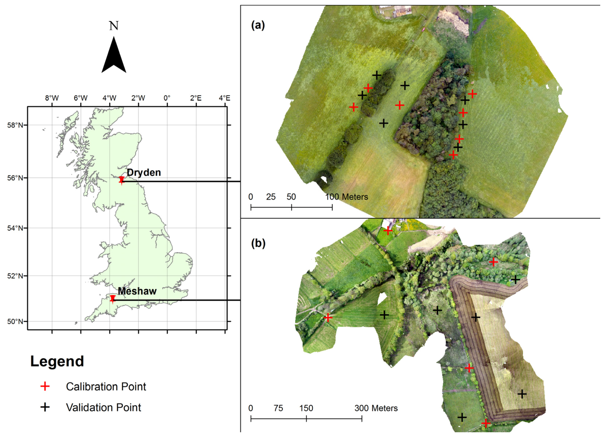
2.1. Test Site and Data Collection
2.2. LiDAR Data
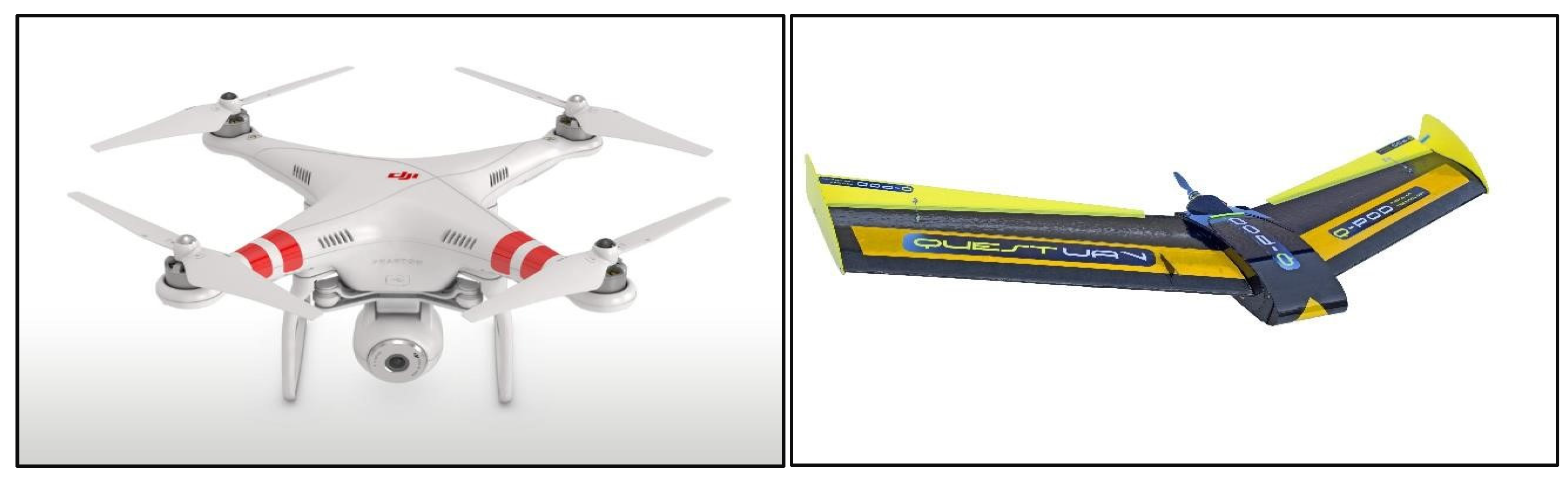
2.3. UAV Surveys
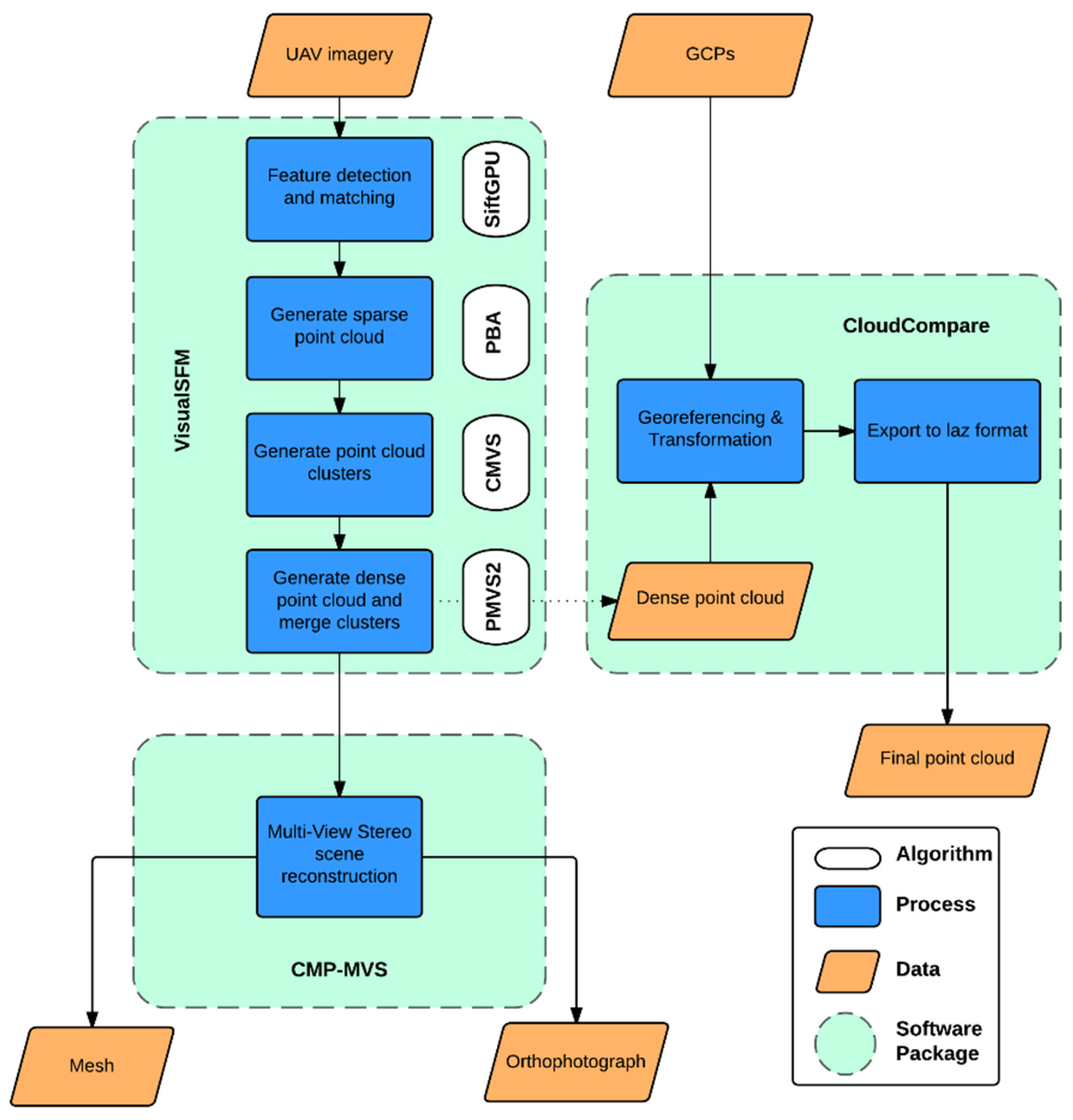
2.4. Structure from Motion and Multi-View Stereo Reconstruction
2.5. Geo-Referencing
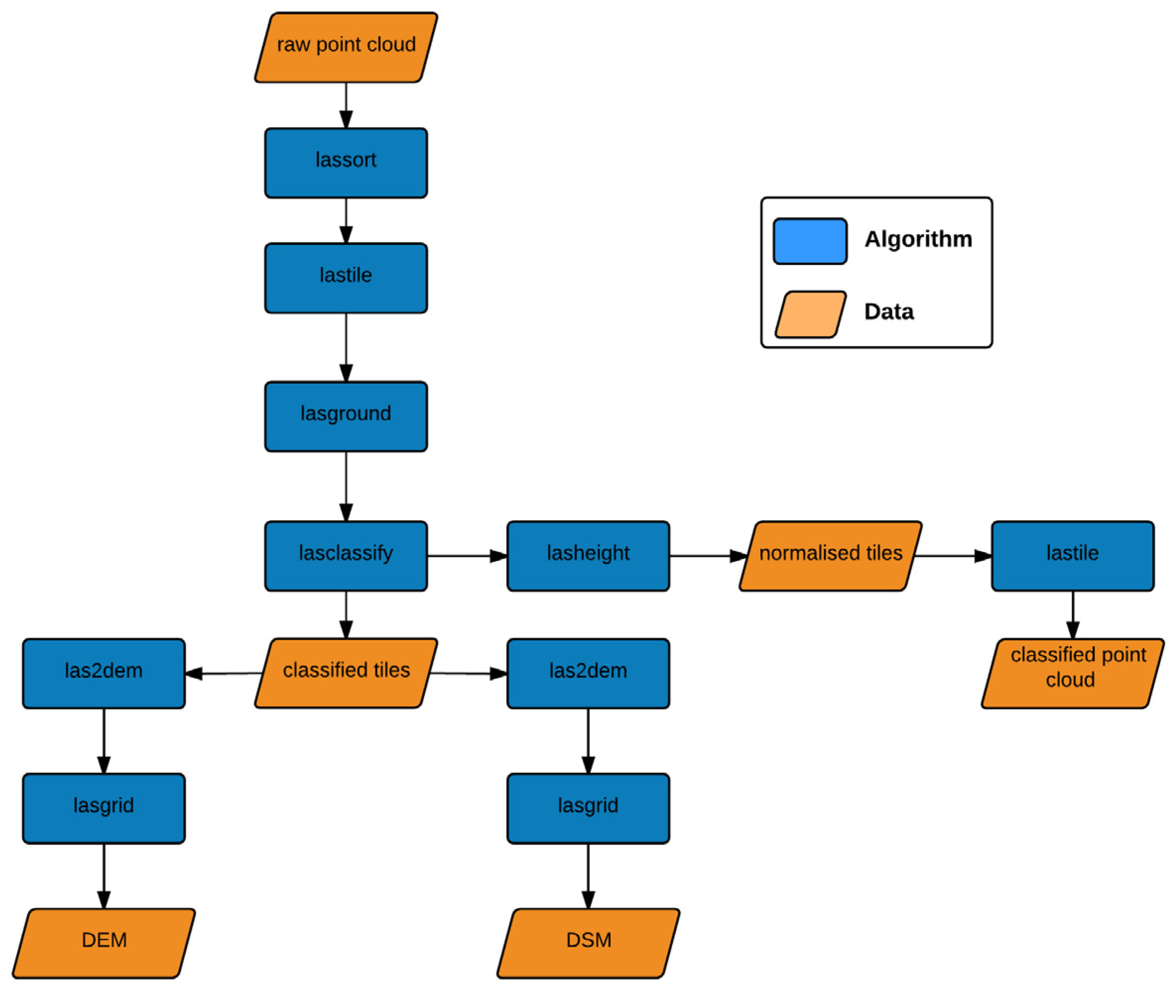
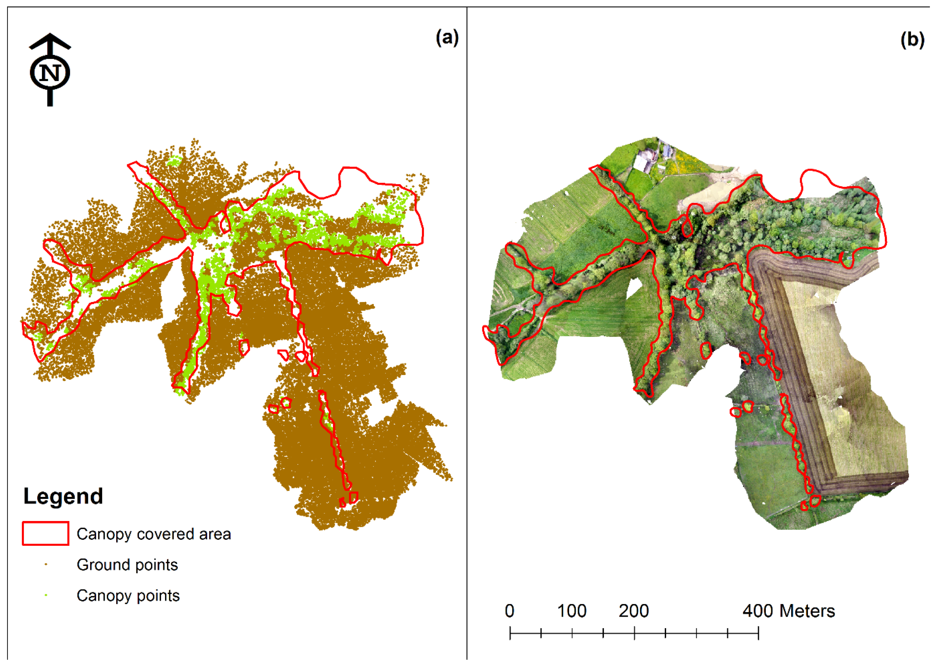
2.6. Point Cloud Post-Processing
3. Results and Discussion
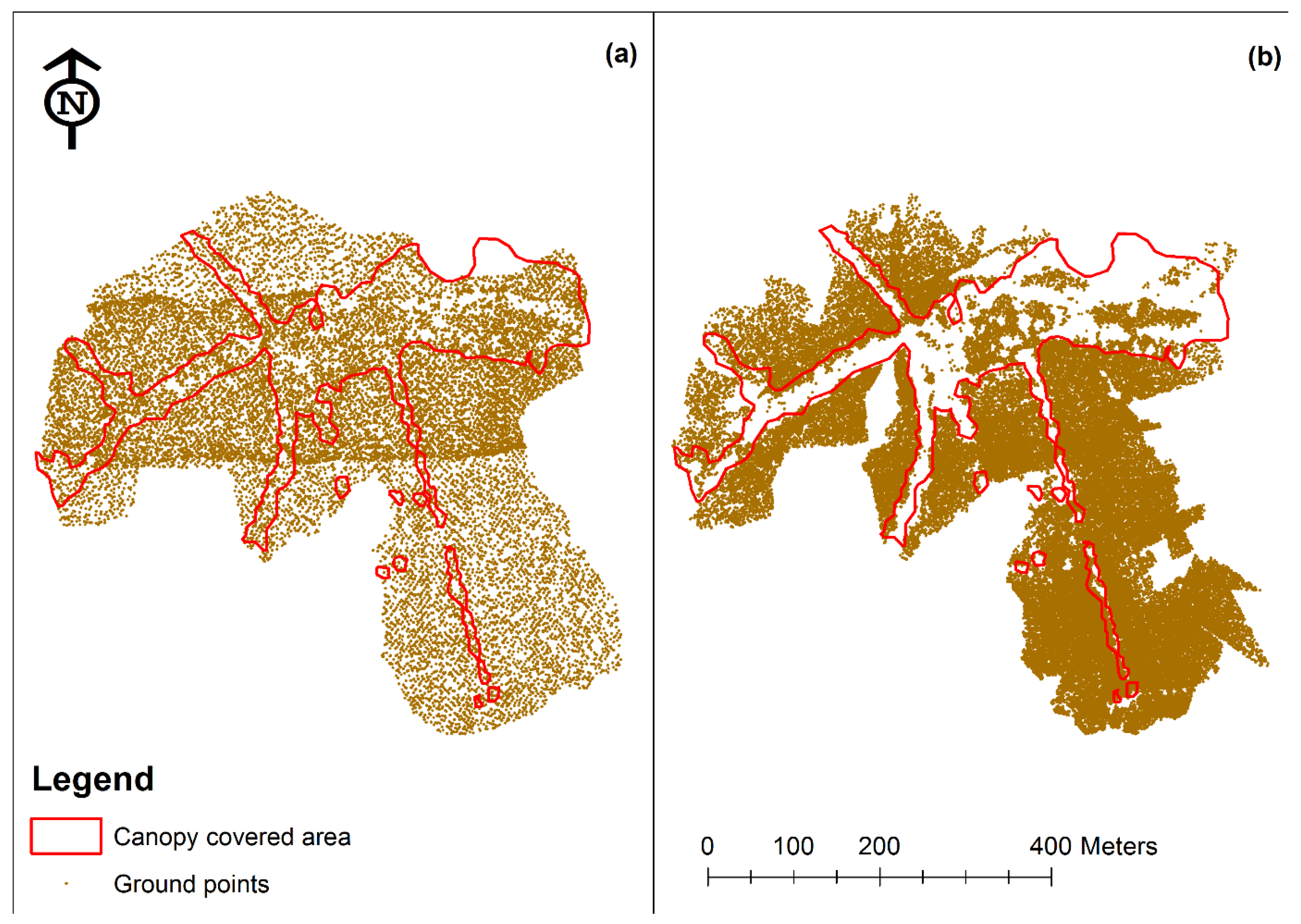
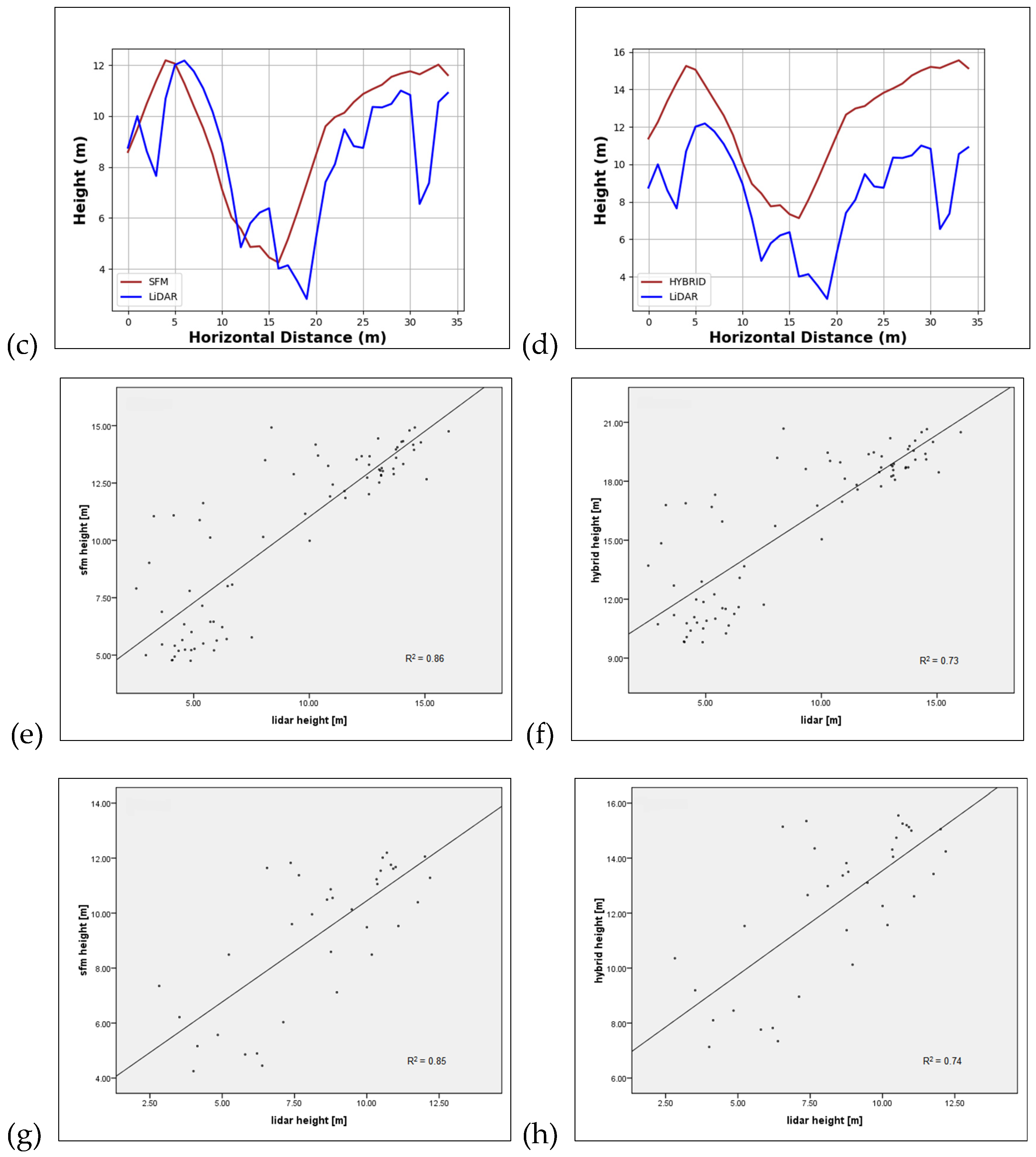
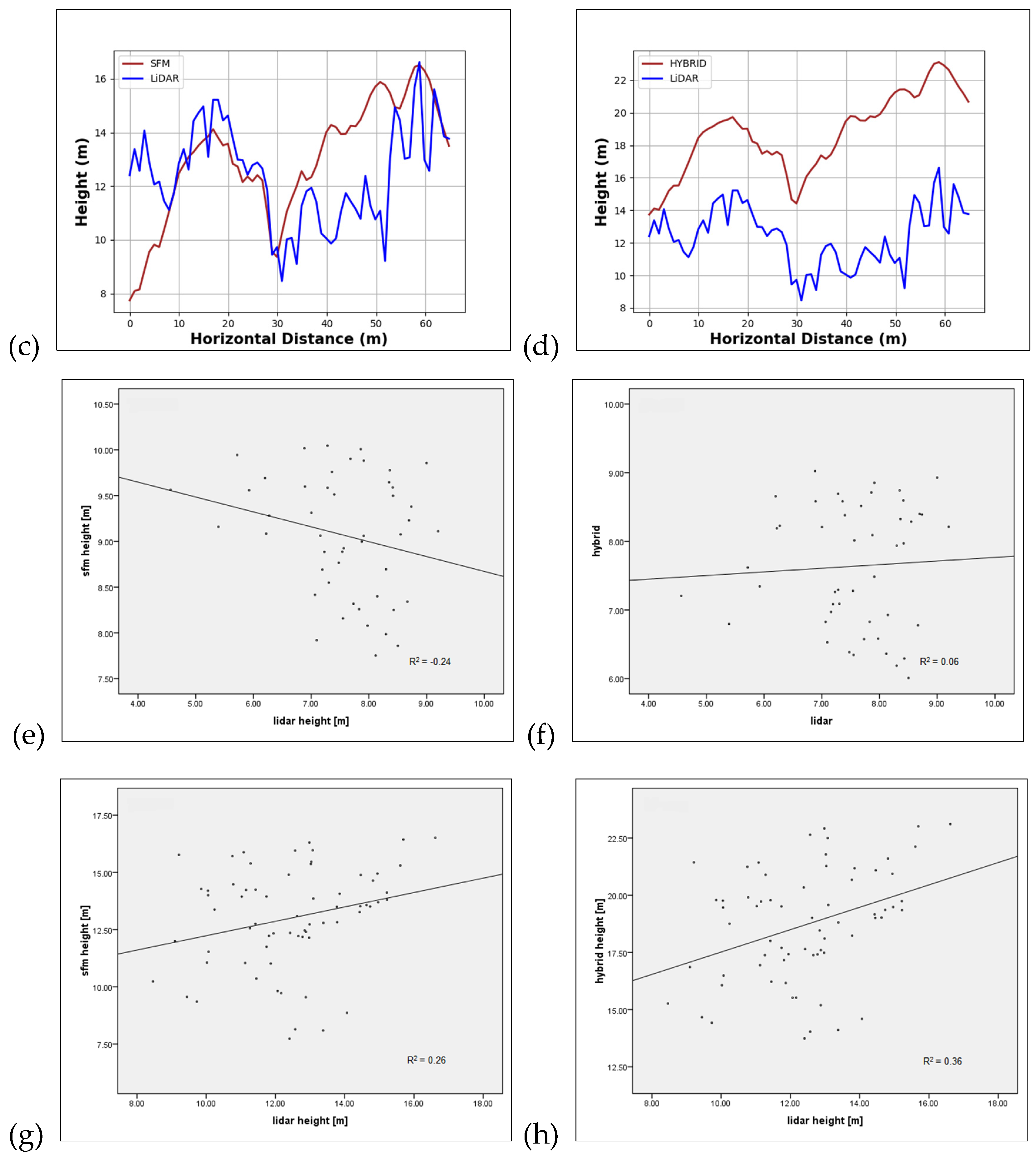
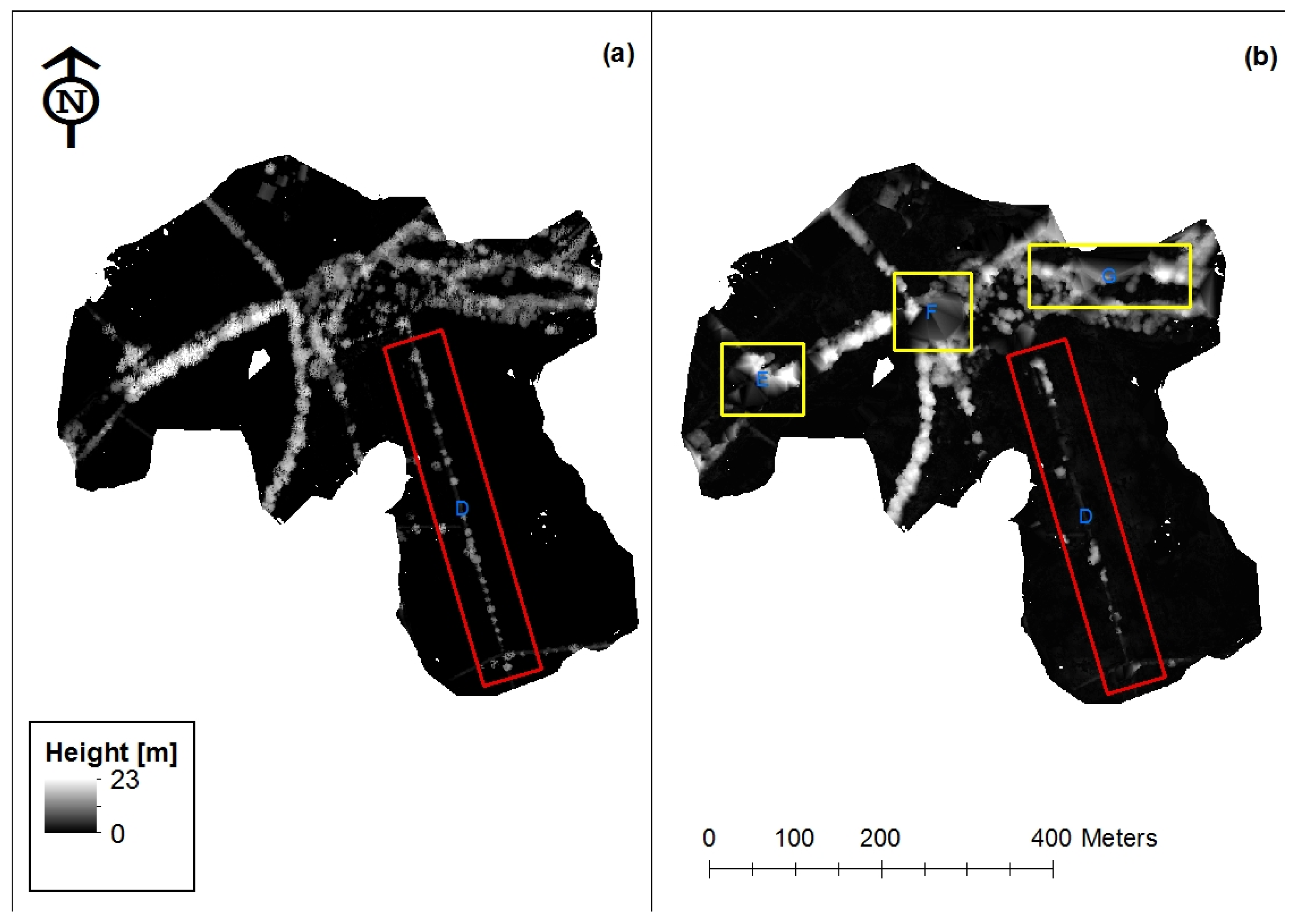
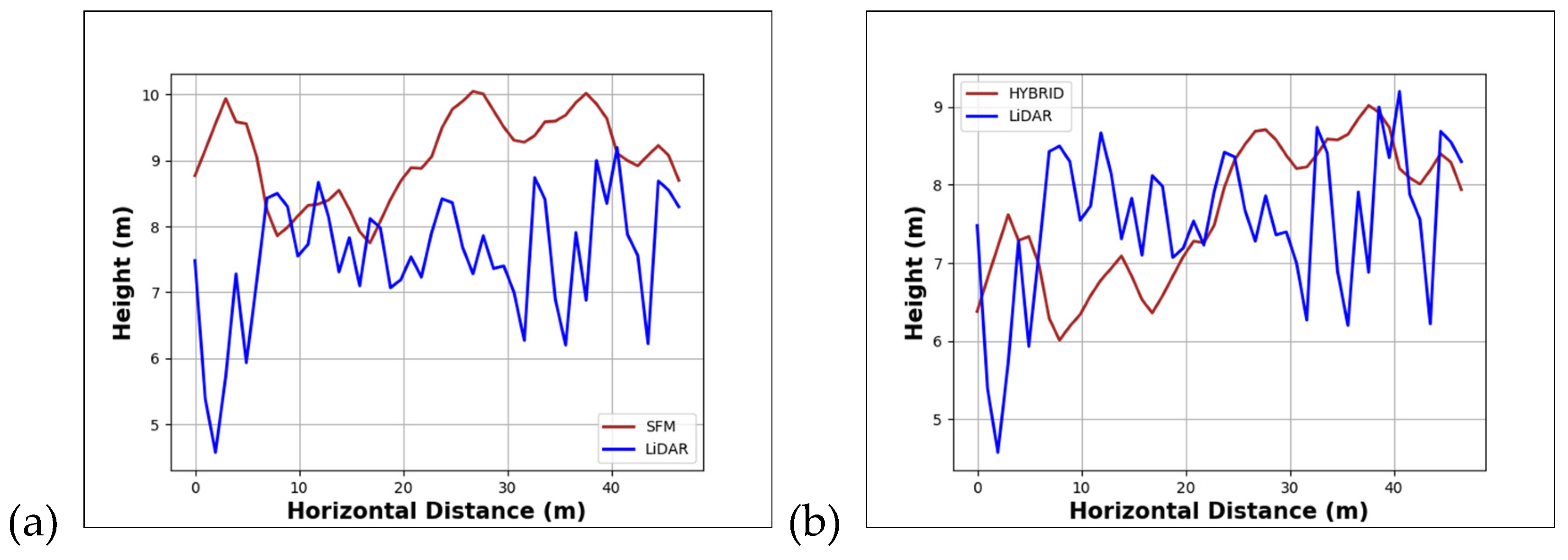
3.1. Point Clouds: Sparse Canopy SfM/Lidar Comparison
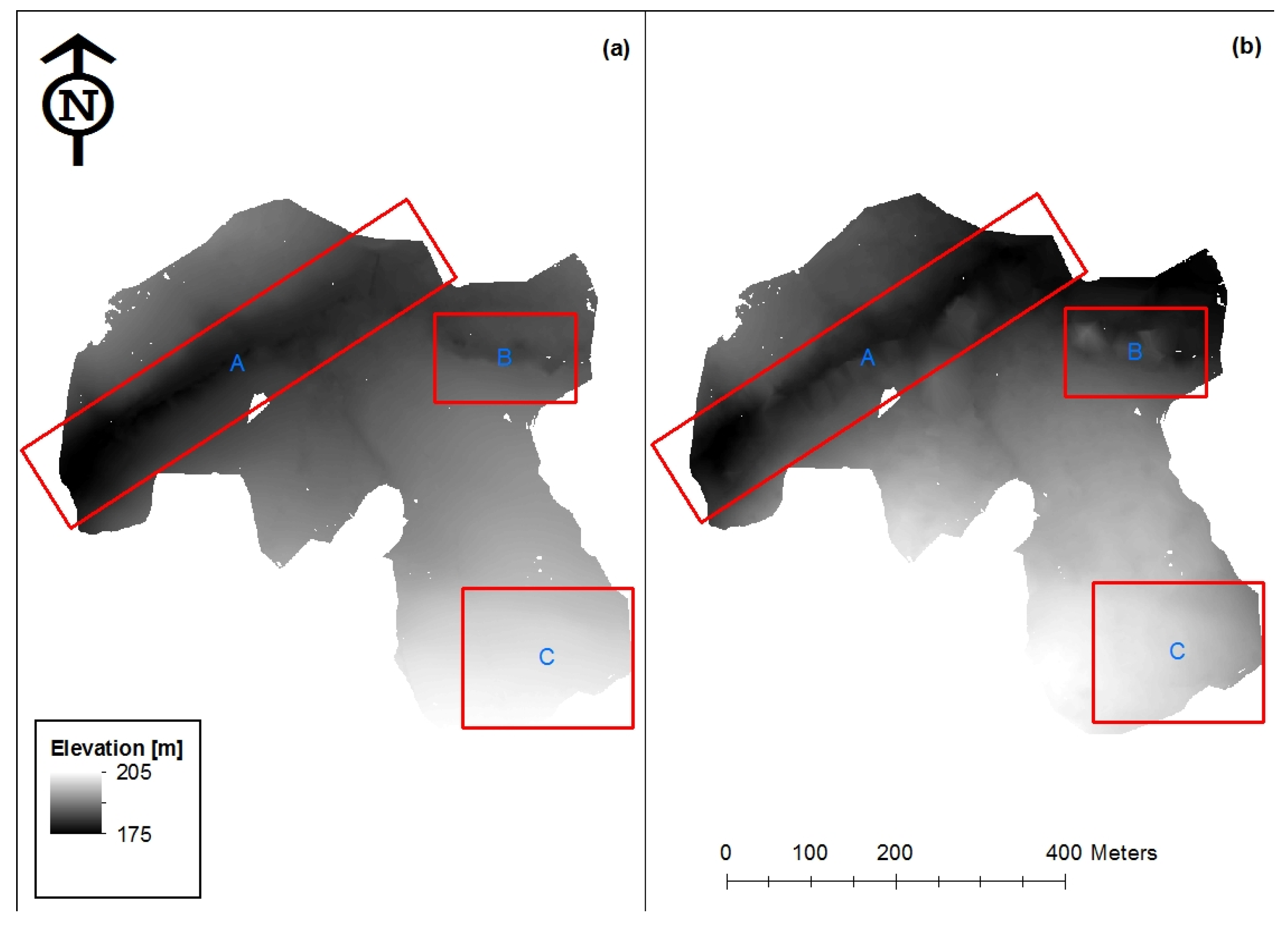
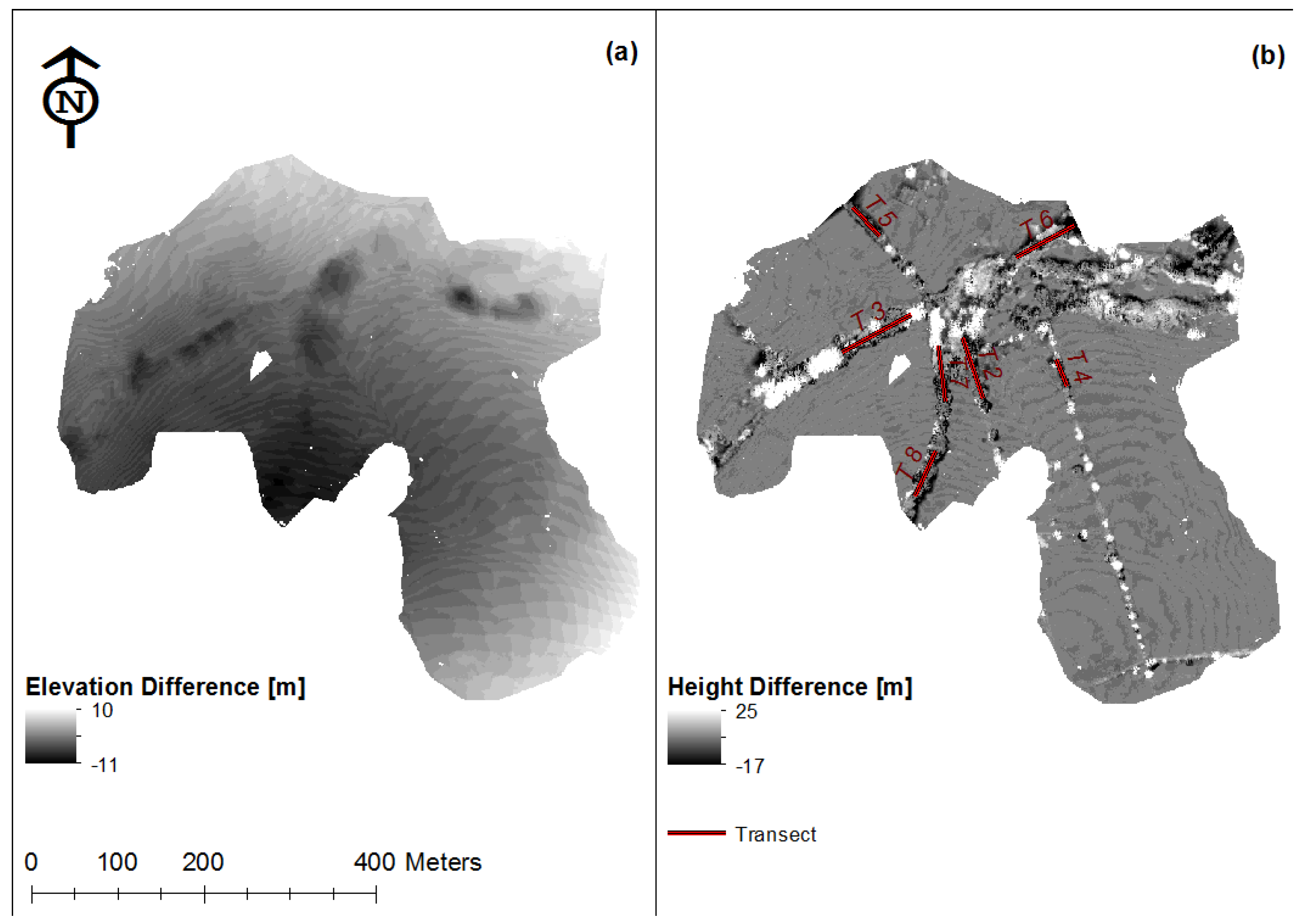
3.2. Digital Elevation Models
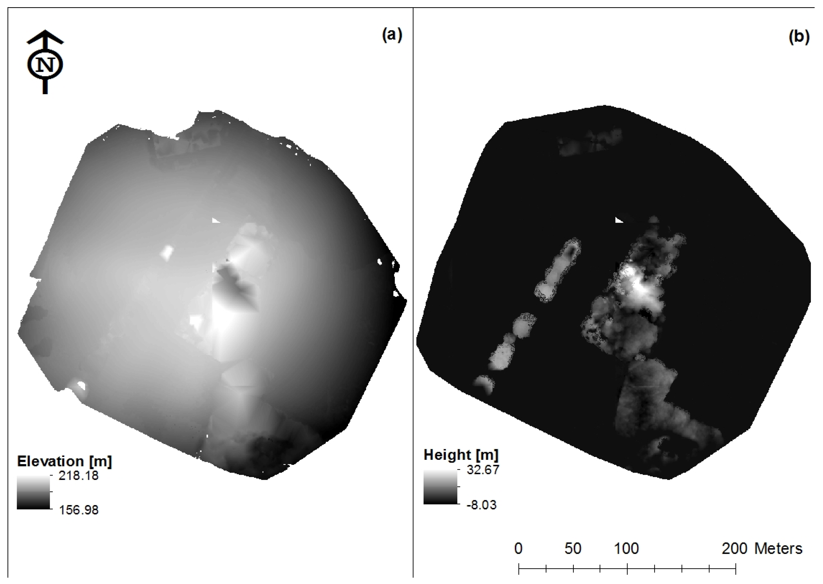
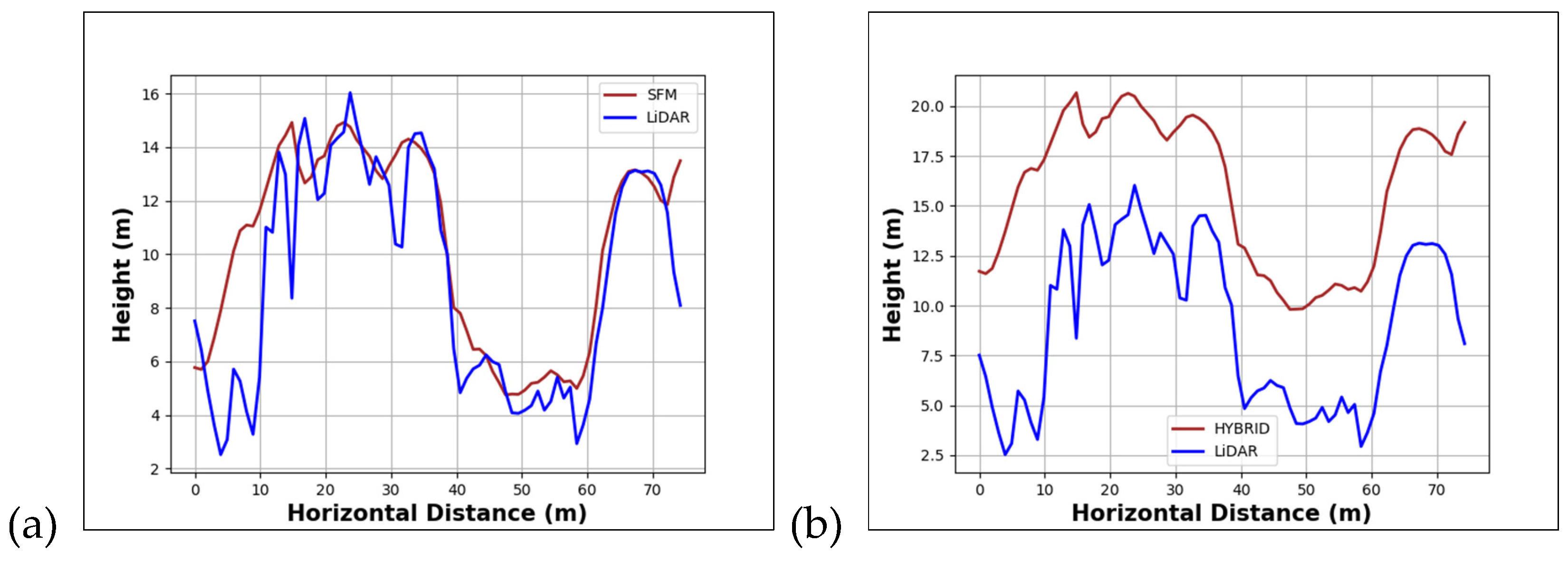
3.3. Canopy Height Models
4. Conclusions
4.1. Challenges with SfM
4.1.1. Accuracy
4.1.2. Canopy Penetration
4.1.3. Data-Richness of Point Clouds
4.2. Small UAVs for Forestry Applications
4.2.1. Ease of Use of UAVs: Missions Flying and Post-Processing
4.2.2. The Cost of Using Small-UAVs
Acknowledgments
Author Contributions
Conflicts of Interest
References
- Brack, D.; Bailey, R. Ending Global Deforestation: Policy Options for Consumer Countries; London Chatham House: London, UK, 2013. [Google Scholar]
- Böttcher, H.; Eisbrenner, K.; Fritz, S.; Kindermann, G.; Kraxner, F.; McCallum, I.; Obersteiner, M. An Assessment of Monitoring Requirements and Costs of “Reduced Emissions from Deforestation and Degradation”. Carbon Balance Manag. 2009, 4, 7. [Google Scholar] [CrossRef] [PubMed]
- Gibbs, H.K.; Brown, S.; Niles, J.O.; Foley, J.A. Monitoring and Estimating Tropical Forest Carbon Stocks: Making REDD a Reality. Environ. Res. Lett. 2007, 2, 45023. [Google Scholar] [CrossRef]
- Herold, M.; Johns, T. Linking Requirements with Capabilities for Deforestation Monitoring in the Context of the UNFCCC-REDD Process. Environ. Res. Lett. 2007, 2, 45025. [Google Scholar] [CrossRef]
- United Nations. UN-REDD Programme Strategy 2011–2015; United Nations: New York, NY, USA, 2011. [Google Scholar]
- Hansen, M.C.; Potapov, P.V.; Moore, R.; Hancher, M.; Turubanova, S.A.; Tyukavina, A.; Thau, D.; Stehman, S.V.; Goetz, S.J.; Loveland, T.R.; et al. High-Resolution Global Maps of 21st-Century Forest Cover Change (15 November): 850–853. Science 2013, 342, 850–853. [Google Scholar] [CrossRef] [PubMed]
- Mitchard, E.T.A.; Saatchi, S.S.; Lewis, S.L.; Feldpausch, T.R.; Gerard, F.F.; Woodhouse, I.H.; Meir, P.; Woodley, E.; Meir, P. Comment on ‘A First Map of Tropical Africa’s above-Ground Biomass Derived from Satellite Imagery’. Environ. Res. Lett. 2011, 6, 49001. [Google Scholar] [CrossRef]
- Snavely, N.; Seitz, S.M.; Szeliski, R. Modeling the World from Internet Photo Collections. Int. J. Comput. Vis. 2008, 80, 189–210. [Google Scholar] [CrossRef]
- Fonstad, M.A.; Dietrich, J.T.; Courville, B.C.; Jensen, J.L.; Carbonneau, P.E. Topographic Structure from Motion: A New Development in Photogrammetric Measurement. Earth Surf. Process. Landf. 2013, 38, 421–430. [Google Scholar] [CrossRef]
- Javernick, L.; Brasington, J.; Caruso, B. Modeling the Topography of Shallow Braided Rivers Using Structure-from-Motion Photogrammetry. Geomorphology 2014, 213, 166–182. [Google Scholar] [CrossRef]
- Mancini, F.; Dubbini, M.; Gattelli, M.; Stecchi, F.; Fabbri, S.; Gabbianelli, G. Using Unmanned Aerial Vehicles (UAV) for High-Resolution Reconstruction of Topography: The Structure from Motion Approach on Coastal Environments. Remote Sens. 2013, 5, 6880–6898. [Google Scholar] [CrossRef] [Green Version]
- Baltsavias, E.; Gruen, A.; Eisenbeiss, H.; Zhang, L.; Waser, L.T. High Quality Image Matching and Automated Generation of 3D Tree Models. Int. J. Remote Sens. 2008, 29, 1243–1259. [Google Scholar] [CrossRef]
- White, J.C.; Wulder, M.A.; Vastaranta, M.; Coops, N.C.; Pitt, D.; Woods, M. The Utility of Image-Based Point Clouds for Forest Inventory: A Comparison with Airborne Laser Scanning. Forests 2013, 4, 518–536. [Google Scholar] [CrossRef]
- Leberl, F.; Irschara, A.; Pock, T.; Meixner, P.; Gruber, M.; Scholz, S.; Wiechert, A. Point Clouds: Lidar versus 3D Vision. Photogramm. Eng. Remote Sens. 2010, 76, 1123–1134. [Google Scholar] [CrossRef]
- St-Onge, B.; Jumelet, J.; Cobello, M.; Véga, C. Measuring Individual Tree Height Using a Combination of Stereophotogrammetry and Lidar. Can. J. For. Res. 2004, 34, 2122–2130. [Google Scholar] [CrossRef]
- Cunliffe, A.M.; Brazier, R.E.; Anderson, K. Ultra-Fine Grain Landscape-Scale Quantification of Dryland Vegetation Structure with Drone-Acquired Structure-from-Motion Photogrammetry. Remote Sens. Environ. 2016, 183, 129–143. [Google Scholar] [CrossRef] [Green Version]
- Messinger, M.; Asner, G.; Silman, M. Rapid Assessments of Amazon Forest Structure and Biomass Using Small Unmanned Aerial Systems. Remote Sens. 2016, 8, 615. [Google Scholar] [CrossRef]
- Dandois, J.P.; Ellis, E.C. Remote Sensing of Vegetation Structure Using Computer Vision. Remote Sens. 2010, 2, 1157–1176. [Google Scholar] [CrossRef]
- Tao, W.; Lei, Y.; Mooney, P. Dense Point Cloud Extraction from UAV Captured Images in Forest Area. In Proceedings of the 2011 IEEE International Conference on Spatial Data Mining and Geographical Knowledge Services (ICSDM 2011), Fuzhou, China, 29 June–1 July 2011; pp. 389–392.
- Lisein, J.; Pierrot-Deseilligny, M.; Bonnet, S.; Lejeune, P. A Photogrammetric Workflow for the Creation of a Forest Canopy Height Model from Small Unmanned Aerial System Imagery. Forests 2013, 4, 922–944. [Google Scholar] [CrossRef]
- Westoby, M.J.; Brasington, J.; Glasser, N.F.; Hambrey, M.J.; Reynolds, J.M. “Structure-from-Motion” Photogrammetry: A Low-Cost, Effective Tool for Geoscience Applications. Geomorphology 2012, 179, 300–314. [Google Scholar] [CrossRef] [Green Version]
- Watts, A.C.; Ambrosia, V.G.; Hinkley, E.A. Unmanned Aircraft Systems in Remote Sensing and Scientific Research: Classification and Considerations of Use. Remote Sens. 2012, 4, 1671–1692. [Google Scholar] [CrossRef]
- Koh, L.P.; Wich, S.A. Dawn of Drone Ecology: Low-Cost Autonomous Aerial Vehicles for Conservation. Trop. Conserv. Sci. 2012, 5, 121–132. [Google Scholar] [CrossRef] [Green Version]
- Civil Aviation Authority. CAP 772: Unmanned Aircraft System Operations in UK Airspace—Guidance; Civil Aviation Authority: Norwich, UK, 2012. [Google Scholar]
- DJI Phantom 2 Vision. Available online: http://quadcopterdump.com/wp-content/uploads/2015/06/phantom-2-vision.jpg (accessed on 21 December 2016).
- Helimetrex and QuestUAV Team up. Available online: https://www.suasnews.com/wp-content/uploads/2014/04/qpod-1024x682.jpg (accessed on 21 December 2016).
- Goetz, S.J.; Dubayah, R. Advances in Remote Sensing Technology and Implications for Measuring and Monitoring Forest Carbon Stocks and Change. Carbon Manag. 2011, 2, 231–244. [Google Scholar] [CrossRef]
- Lloyd, C.R.; Rebelo, L.-M.; Max Finlayson, C. Providing Low-Budget Estimations of Carbon Sequestration and Greenhouse Gas Emissions in Agricultural Wetlands. Environ. Res. Lett. 2013, 8, 15010–15013. [Google Scholar] [CrossRef]
- Cho, M.A.; Skidmore, A.; Corsi, F.; van Wieren, S.E.; Sobhan, I. Estimation of Green Grass/herb Biomass from Airborne Hyperspectral Imagery Using Spectral Indices and Partial Least Squares Regression. Int. J. Appl. Earth Obs. Geoinf. 2007, 9, 414–424. [Google Scholar] [CrossRef]
- Thenkabail, P.S.; Enclona, E.A.; Ashton, M.S.; Legg, C.; de Dieu, M.J. Hyperion, IKONOS, ALI, and ETM+ Sensors in the Study of African Rainforests. Remote Sens. Environ. 2004, 90, 23–43. [Google Scholar] [CrossRef]
- Koch, B. Status and Future of Laser Scanning, Synthetic Aperture Radar and Hyperspectral Remote Sensing Data for Forest Biomass Assessment. ISPRS J. Photogramm. Remote Sens. 2010, 65, 581–590. [Google Scholar] [CrossRef]
- Gerstl, S.A.W. Physics Concepts of Optical and Radar Reflectance Signatures A Summary Review. Int. J. Remote Sens. 1990, 11, 1109–1117. [Google Scholar] [CrossRef]
- Harrell, P.A.; Bourgeau-Chavez, L.L.; Kasischke, E.S.; French, N.H.F.; Christensen, N.L. Sensitivity of ERS-1 and JERS-1 Radar Data to Biomass and Stand Structure in Alaskan Boreal Forest. Remote Sens. Environ. 1995, 54, 247–260. [Google Scholar] [CrossRef]
- Craig Dobson, M.; Ulaby, F.T.; Pierce, L.E. Land-Cover Classification and Estimation of Terrain Attributes Using Synthetic Aperture Radar. Remote Sens. Environ. 1995, 51, 199–214. [Google Scholar] [CrossRef]
- Freeman, A.; Durden, S.L. A Three-Component Scattering Model for Polarimetric SAR Data. IEEE Trans. Geosci. Remote Sens. 1998, 36, 963–973. [Google Scholar] [CrossRef]
- Lu, D. The Potential and Challenge of Remote Sensing-based Biomass Estimation. Int. J. Remote Sens. 2006, 27, 1297–1328. [Google Scholar] [CrossRef]
- Li, W.; Guo, Q.; Jakubowski, M.K.; Kelly, M. A New Method for Segmenting Individual Trees from the Lidar Point Cloud. Photogramm. Eng. Remote Sens. 2012, 78, 75–84. [Google Scholar] [CrossRef]
- Zhao, K.; Popescu, S.; Nelson, R. Lidar Remote Sensing of Forest Biomass: A Scale-Invariant Estimation Approach Using Airborne Lasers. Remote Sens. Environ. 2009, 113, 182–196. [Google Scholar] [CrossRef]
- Lefsky, M.A.; Cohen, W.B.; Parker, G.G.; Harding, D.J. Lidar Remote Sensing for Ecosystem Studies. Bioscience 2002, 52, 19–30. [Google Scholar] [CrossRef]
- Hummel, S.; Hudak, A.T.; Uebler, E.H.; Falkowski, M.J.; Megown, K.A. A Comparison of Accuracy and Cost of LiDAR versus Stand Exam Data for Landscape Management on the Malheur National Forest. J. For. 2011, 109, 267–273. [Google Scholar]
- Takasu, T. RTKLIB: An Open Source Program Package for GNSS Positioning. Available online: http://www.rtklib.com/ (accessed on 15 July 2015).
- The Tellus South West Project. Available online: http://www.tellusgb.ac.uk/ (accessed 10 June 2015).
- Ferraccioli, F.; Gerard, F.; Robinson, C.; Jordan, T.; Biszczuk, M.; Ireland, L.; Beasley, M.; Vidamour, A.; Barker, A.; Arnold, R.; et al. LiDAR Based Digital Terrain Model (DTM) Data for South West England. Available online: https://doi.org/10.5285/e2a742df-3772-481a-97d6-0de5133f4812 (accessed on 10 June 2015).
- Ferraccioli, F.; Gerard, F.; Robinson, C.; Jordan, T.; Biszczuk, M.; Ireland, L.; Beasley, M.; Vidamour, A.; Barker, A.; Arnold, R.; et al. LiDAR based Digital Surface Model (DSM) data for South West England. Available online: https://doi.org/10.5285/b81071f2-85b3-4e31-8506-cabe899f989a (accessed on 10 June 2015).
- James, M.R.; Robson, S. Mitigating Systematic Error in Topographic Models Derived from UAV and Ground-Based Image Networks. Earth Surf. Process. Landf. 2014, 39, 1413–1420. [Google Scholar] [CrossRef]
- Paull, L.; Thibault, C.; Nagaty, A.; Seto, M.; Li, H. Sensor-Driven Area Coverage for an Autonomous Fixed-Wing Unmanned Aerial Vehicle. IEEE Trans. Cybern. 2014, 44, 1605–1618. [Google Scholar] [CrossRef] [PubMed]
- DJI. Phantom 2 User Manual v1.2. Available online: http://download.dji-innovations.com/downloads/phantom_2/en/PHANTOM2_User_Manual_v1.2_en.pdf (accessed on 1 July 2015).
- Wu, C. Towards Linear-Time Incremental Structure from Motion. In Proceedings of the 2013 International Conference on 3D Vision, 3DV 2013, Seattle, WA, USA, 29 June–1 July 2013; pp. 127–134.
- Jancosek, M.; Pajdla, T. Multi-View Reconstruction Preserving Weakly-Supported Surfaces. In Proceedings of the IEEE Computer Society Conference on Computer Vision and Pattern Recognition, Colorado Springs, CO, USA, 20–25 June 2011; pp. 3121–3128.
- Wu, C. VisualSFM: A Visual Structure from Motion System. Available online: http://ccwu.me/vsfm/ (accessed on 15 July 2015).
- Lowe, D.G. Object Recognition from Local Scale-Invariant Features. In Proceedings of the Seventh IEEE International Conference on Computer Vision, Kerkyra, Greece, 20–27 September 1999; Volume 2, pp. 1150–1157.
- Lowe, D.G. Distinctive Image Features from Scale-Invariant Keypoints. Int. J. Comput. Vis. 2004, 60, 91–110. [Google Scholar] [CrossRef]
- Furukawa, Y.; Ponce, J. Accurate, Dense, and Robust Multiview Stereopsis. IEEE Trans. Pattern Anal. Mach. Intell. 2010, 32, 1362–1376. [Google Scholar] [CrossRef] [PubMed]
- Besl, P.J.; McKay, N.D. Method for Registration of 3-D Shapes. IEEE Trans. Pattern Anal. Mach. Intell. 1992, 14, 239–256. [Google Scholar] [CrossRef]
- Rapidlasso. LAStools: Converting, Filtering, Viewing, Processing and Compressing LiDAR Data in LAS Format. Available online: http://www.cs.unc.edu/~isenburg/lastools/ (accessed on 4 August 2015).
- Isenburg, M.; Liu, Y.; Shewchuk, J.; Snoeyink, J. Streaming Computation of Delaunay Triangulations. ACM Siggraph 2006, 25, 1049–1056. [Google Scholar] [CrossRef]
- Isenburg, M.; Liu, Y.; Shewchuk, J.; Snoeyink, J.; Thirion, T. Generating Raster DEM from Mass Points via TIN Streaming. Geogr. Inf. Sci. 2006, 4197, 186–198. [Google Scholar]
- Lingua, A.; Marenchino, D.; Nex, F. Performance Analysis of the SIFT Operator for Automatic Feature Extraction and Matching in Photogrammetric Applications. Sensors 2009, 9, 3745–3766. [Google Scholar] [CrossRef] [PubMed]
- Girardeau-Montaut, D.; Roux, M.; Marc, R.; Thibault, G. Change Detection on Points Cloud Data Acquired with a Ground Laser Scanner. Int. Arch. Photogramm. Remote Sens. Spat. Inf. Sci. 2005, 36, W19. [Google Scholar]
- Khosravipour, A.; Skidmore, A.K.; Isenburg, M.; Wang, T.; Hussin, Y.A. Generating Pit-Free Canopy Height Models from Airborne Lidar. Photogramm. Eng. Remote Sens. 2014, 80, 863–872. [Google Scholar] [CrossRef]
- Jakubowski, M.K.; Guo, Q.; Kelly, M. Tradeoffs between Lidar Pulse Density and Forest Measurement Accuracy. Remote Sens. Environ. 2013, 130, 245–253. [Google Scholar] [CrossRef]
- Puttock, A.K.; Cunliffe, A.M.; Anderson, K.; Brazier, R.E. Aerial Photography Collected with a Multirotor Drone Reveals Impact of Eurasian Beaver Reintroduction on Ecosystem Structure 1. J. Unmanned Veh. Syst. 2015, 3, 123–130. [Google Scholar] [CrossRef]
- Paneque-Gálvez, J.; McCall, M.K.; Napoletano, B.M.; Wich, S.A.; Koh, L.P. Small Drones for Community-Based Forest Monitoring: An Assessment of Their Feasibility and Potential in Tropical Areas. Forests 2014, 5, 1481–1507. [Google Scholar] [CrossRef]
- Eisenbeiß, H. UAV Photogrammetry; ETH Zurich: Zurich, Switzerland, 2009. [Google Scholar]
- Estrada Porrúra, M.; Corbera, E.; Brown, K. Reducing Greenhouse Gas Emissions from Deforestation in Developing Countries: Revisiting the Assumptions. Clim. Chang. 2007, 100, 355–388. [Google Scholar]


| Site | UAV | Camera | Flying Height (m) | Flying Speed [m/s] | Ground Sampling Distance (cm) | No. of Photos |
|---|---|---|---|---|---|---|
| Meshaw | Quest QPod | Sony NEX-7 | 100 | 14 (average) | 1.66 | 111 |
| Dryden | DJI Phantom | GoPro Hero 3+ | 100 and 50 | 5 | 3.57 | 999 |
| Site | Validation GCPs | Check Points | RMSE (m) | |
|---|---|---|---|---|
| Horizontal | Vertical | |||
| Meshaw | 5 | 6 | 2.53 | 3.05 |
| Dryden | 7 | 7 | 1.77 | 2.01 |
| Criterion | Strength | Weakness |
|---|---|---|
| Accuracy | Performs well over bare ground. | Performs poorly with poor image coverage. |
| Cost | Cost-effective for small areas. Cheap hobbyist UAVs available (e.g., the one used in [16]). Open source SfM/MVS software available. | Open source might not be as accurate as commercial software. Cheap camera models (e.g., GoPro) introduce large distortions in SfM models. |
| Ease of use/Learning curve | Full autonomous missions. Automated data processing. | Post-processing still requires experienced users. |
| Amount of data | High density point clouds. Easy interpretation of point cloud because of true colour rendering. | Classification of points based only on point height (no return number). |
© 2017 by the authors. Licensee MDPI, Basel, Switzerland. This article is an open access article distributed under the terms and conditions of the Creative Commons Attribution (CC BY) license ( http://creativecommons.org/licenses/by/4.0/).
Share and Cite
Mlambo, R.; Woodhouse, I.H.; Gerard, F.; Anderson, K. Structure from Motion (SfM) Photogrammetry with Drone Data: A Low Cost Method for Monitoring Greenhouse Gas Emissions from Forests in Developing Countries. Forests 2017, 8, 68. https://doi.org/10.3390/f8030068
Mlambo R, Woodhouse IH, Gerard F, Anderson K. Structure from Motion (SfM) Photogrammetry with Drone Data: A Low Cost Method for Monitoring Greenhouse Gas Emissions from Forests in Developing Countries. Forests. 2017; 8(3):68. https://doi.org/10.3390/f8030068
Chicago/Turabian StyleMlambo, Reason, Iain H. Woodhouse, France Gerard, and Karen Anderson. 2017. "Structure from Motion (SfM) Photogrammetry with Drone Data: A Low Cost Method for Monitoring Greenhouse Gas Emissions from Forests in Developing Countries" Forests 8, no. 3: 68. https://doi.org/10.3390/f8030068