
Spatial Heterogeneity of the Forest Canopy Scales with the Heterogeneity of an Understory Shrub Based on Fractal Analysis


Department of Renewable Resources, University of Alberta, 751 General Services Building, Edmonton, AB T6G 2H1, Canada
*
Author to whom correspondence should be addressed.
Forests 2017, 8(5), 146; https://doi.org/10.3390/f8050146
Submission received: 15 February 2017
/
Revised: 21 April 2017
/
Accepted: 25 April 2017
/
Published: 27 April 2017
(This article belongs to the Special Issue Successional Dynamics of Forest Structure and Function)
Abstract
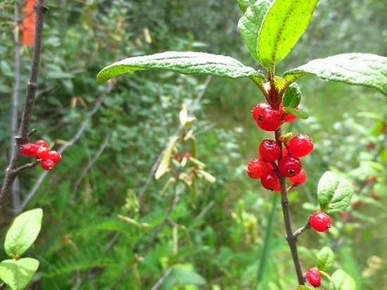
:Spatial heterogeneity of vegetation is an important landscape characteristic, but is difficult to assess due to scale-dependence. Here we examine how spatial patterns in the forest canopy affect those of understory plants, using the shrub Canada buffaloberry (Shepherdia canadensis (L.) Nutt.) as a focal species. Evergreen and deciduous forest canopy and buffaloberry shrub presence were measured with line-intercept sampling along ten 2-km transects in the Rocky Mountain foothills of west-central Alberta, Canada. Relationships between overstory canopy and understory buffaloberry presence were assessed for scales ranging from 2 m to 502 m. Fractal dimensions of both canopy and buffaloberry were estimated and then related using box-counting methods to evaluate spatial heterogeneity based on patch distribution and abundance. Effects of canopy presence on buffaloberry were scale-dependent, with shrub presence negatively related to evergreen canopy cover and positively related to deciduous cover. The effect of evergreen canopy was significant at a local scale between 2 m and 42 m, while that of deciduous canopy was significant at a meso-scale between 150 m and 358 m. Fractal analysis indicated that buffaloberry heterogeneity positively scaled with evergreen canopy heterogeneity, but was unrelated to that of deciduous canopy. This study demonstrates that evergreen canopy cover is a determinant of buffaloberry heterogeneity, highlighting the importance of spatial scale and canopy composition in understanding canopy-understory relationships.

1. Introduction
Spatial heterogeneity is both a product [1] and determinant of ecological processes, and is thus an important landscape property [2,3]. Spatial heterogeneity is, however, difficult to quantify [4,5] as it is scale-dependent [4,6,7]. For vegetation, spatial heterogeneity can be defined as the variance in the horizontal distribution of plants determined by both the dispersion of patches and contrast between vegetation types or species [8]. Vegetation patterns are collectively shaped by a series of interactions between climate, terrain, soil, biotic factors, and disturbance processes [9,10,11,12].
Spatial patterns in forests are affected by both natural and anthropogenic disturbances, such as timber harvesting, which modify the size and arrangement of tree patches [13]. Disturbance therefore creates variability in the horizontal structure of the canopy and is an important factor affecting vegetation heterogeneity [9,11,12]. The severity of landscape disturbance may be inferred by examining the distribution of vegetation patch sizes and the degree to which this deviates from a power law relationship, with greater divergence indicating more extensive disturbance [14]. Variation in the forest canopy also exerts strong influences on understory microhabitats through the regulation of key above- and below-ground resources, such as light [15] and soil nutrients [16,17], which control plant growth and survival [18,19].
Resource quantity and heterogeneity both structure understory plant patterns, with the latter demonstrated to be especially relevant for disturbed stands [20]. Canopy composition alters resource availability in the understory [21], suggesting that the effect of the canopy differs between evergreen and deciduous trees [16,22,23]. Evergreen canopies may transmit less light [24,25], although this is species-dependent and dictated by factors such as shade-tolerance [26,27,28] and successional status [24,25,29], which consequently affect leaf area and crown architecture [27,30].
These resource-related interactions between canopy and understory produce linkages between their respective spatial patterns [16,31,32,33], which vary between evergreen- and deciduous-dominated stands [23]. In particular, the presence of evergreen conifers has been identified as a key determinant of understory patterns [16,34,35], the heterogeneity of which may increase with conifer abundance [23]. The strength and direction of canopy-understory spatial relationships are scale-dependent [23,36], as the local influence of an individual tree on nearby understory plants is distinct from the collective effect of numerous trees over a larger area [36]. However, despite the importance of multi-scale analyses for better understanding spatial dynamics between the canopy and understory, assessments across scales are uncommon.
Fractal analysis is an inherently multi-scale approach for characterizing spatial patterns [6] and is particularly useful for addressing issues of scale [37,38]. Rarely, however, has this been applied to spatial overstory-understory relationships (however, see [39] for a multi-scale wavelet approach that related understory plant patterns to overstory composition and structure). Unlike exact fractals that are perfectly self-similar, natural fractals demonstrate statistical self-similarity across a limited range of spatial scales [40,41] which may amount to several orders of magnitude [42,43]. A power law will apply within the range of self-similarity, and this type of relationship has been recognized as a tool for clarifying the organization of complex ecological systems given its scale-invariance that can facilitate extrapolation [44].
Fractal properties of a pattern can be evaluated by calculating the fractal dimension (D) which summarizes complexity and space-filling ability with one succinct, non-integer value [6]. The box-counting method is one of multiple approaches for estimating D [43,45,46], which considers the number of grid segments occupied by a material across different spatial scales. When the number of occupied segments is regressed against the segment or “box” width on a log-log plot, D can be calculated with the equation [47]:
slope = 1 − D,
A natural pattern is fractal-like over the spatial range where a power law holds, which is characterized by a linear relationship on a log-log plot [44].
For a material distributed across a two-dimensional plane, such as an aerial view of a landscape, D will range between 0 and 2; a value of 0 is a single point, 1 suggests high self-similarity and clustering, and 2 denotes a complete random distribution [43]. Box-counting can be performed using line-intercept transect data to calculate D of vegetation patterns [48], with each transect representing a linear arrangement of segments that effectively subsample the broader landscape, such that 0 < D < 2 [47,49]. These transect data reflect both patch size and distribution, which are pertinent aspects of horizontal vegetation heterogeneity. D is affected by the amount and dispersion of a material across the landscape [50], and is thus altered by variation in the size and distribution of vegetation patches.
D is an indicator of pattern homogeneity [31], which can be defined as the randomness of a distribution [3]. Pattern randomness increases as D approaches 2 [3,31], and therefore a lower D signifies greater heterogeneity. The value of D may change with the experimental scale [31] and is not an absolute measure of heterogeneity; however, examining measures of forest canopy and understory cover at the same scale facilitates a relative comparison of their patterns [51]. Fractal analyses of forest vegetation have mainly assessed attributes such as patch shape [52,53,54] and canopy height [55,56] rather than heterogeneity as defined here. Studies often rely on remote sensing data to calculate D and utilize methods such as perimeter-area ratios [52,53,54], semivariograms [56], and multifractals [55].
Most applications of box-counting to research on vegetation patterns have focused on individual plant structure [57,58,59,60] rather than landscape patterns of plants or interactions between different landscape elements. Studies that have employed box-counting to analyze plant distributions have also generally focused on species in non-forested ecosystems, such as crested wheatgrass (Agropyron desertorum (Fisch. ex Link) Schult.) in grasslands or big sagebrush (Artemisia tridentata Nutt.) in shrub lands [48]. Rarely has this technique been used in the more vertically complex systems of forests, although field measurements are straightforward and can be obtained at a fine resolution (e.g., centimeters or decimeters). Box-counting along transects also allows for measures of other attributes, like species composition, to be collected that are difficult to discern accurately with remote sensing data. Evaluating relationships between canopy and understory heterogeneity, using fractal metrics such as D, can provide important insights into the spatial dynamics of forest vegetation strata at scales beyond the individual forest stand (i.e., landscape-level). In this study, we compare spatial patterns of the overstory forest with those of a common shrub in a montane forested ecosystem in the foothills of Alberta, Canada. Canada buffaloberry (Shepherdia canadensis (L.) Nutt.) is a shade-intolerant [61], dioecious shrub that occurs in boreal and temperate montane forests [62,63] across Canada and the northern United States [64] and flowers in early spring [65]. The effects of canopy on buffaloberry have been examined previously, but the focus has been on fruit production [66,67] with no differences considered between evergreen and deciduous canopy types.
Our focus here is to examine relationships between landscape patterns of forest canopy and buffaloberry, in terms of presence and heterogeneity, across multiple spatial scales and forest cover gradients. Specifically, we have two main objectives: first, to determine the total and individual effects of evergreen and deciduous canopy cover on buffaloberry presence across multiple orders of scale, and second, to use fractal box-counting to evaluate relationships between the heterogeneity of canopy cover (evergreen vs. deciduous) and that of buffaloberry patches.
We hypothesize that, given differences in resource regulation, evergreen and deciduous canopy will demonstrate distinct effects on the presence and patterns of buffaloberry, which will vary with spatial scale due to changes in resource availability in space. Following this, we hypothesize that greater canopy heterogeneity (lower D) will be associated with greater buffaloberry heterogeneity, because the patterns of the overstory forest should structure those of understory plants. We expect, however, that evergreen canopy will have a stronger effect on buffaloberry presence and heterogeneity than deciduous canopy, due to generally lower light conditions under some evergreen species common to our study area; this could limit buffaloberry growth and reproductive success, as shrubs flower prior to leaf emergence in deciduous trees [65].
2. Materials and Methods
2.1. Study Area
The study area covers 2389 km2 of managed, conifer-dominated forest southeast of the town of Hinton (53°24′41″ N, 117°33′50″ W) and north of the town of Robb (53°13′59″ N, 116°58′42″ W) in the Rocky Mountain foothills of west-central Alberta (Figure 1). The climate is moist and cool [68], with higher elevation in the west that declines in the east across a range from 950 m to 2500 m. Land cover types include evergreen, deciduous, and mixed forest consisting of dominant tree species such as lodgepole pine (Pinus contorta Douglas ex Loudon), white spruce (Picea glauca (Moench) Voss), and trembling aspen (Populus tremuloides Michx.) [68,69]. Open bogs, meadows, and previously harvested cutblocks are also present on the landscape. Active resource extraction and development by the forestry, mining, and energy (oil and gas) industries has resulted in varying degrees of anthropogenic disturbance.
2.2. Site Selection
Field sites were selected using canopy cover estimates derived from airborne light detection and ranging (LiDAR) data (2005–2007) [70], scaled at a resolution of 25 m. These data were used to stratify the landscape for sampling into three ordinal canopy cover categories defined by the proportion of the forest floor covered by tree crowns [15]: low (0–40% cover), moderate (40–55%), and high (>55%). Each canopy cover category was subsequently divided into low, medium, and high canopy variability levels based on the standard deviation of canopy cover, which was quantile binned in a Geographic Information System (GIS) [71]. To determine the appropriate transect length for obtaining box-counting measurements in the field, neighbourhood analyses were performed to examine changes in average variability in canopy cover as the moving “window” size (scale) was sequentially increased. This process indicated that a transect length of 2 km would both represent a range of canopy conditions and enable sampling efficiency in the field. A total of ten transect replicates were sited using a stratified random sampling design. Replicates were balanced among canopy variability levels, with three placed in each of the low and high canopy cover categories and four in the moderate cover category. The mean distance among selected transects was 19.9 km, with a maximum and minimum distance of 41.6 km and 4 km, respectively.
2.3. Field Methods
The ten 2-km transects were established in the field based on randomized starting locations and orientations. Dominant forest canopy species and land cover type were noted for each transect, which included upland forest, wet forest, and cutblocks at various stages of regeneration. Line-intercept was used to measure the length of buffaloberry shrub intercepts along the transect tape at a 0.01-m resolution, resulting in 200,000 recorded segments (binary presence-absence conditions) per transect. Intercept length was evaluated per shrub and recorded as the maximum extent of an individual along the transect line, with no differentiation made between female and male shrubs; it was not feasible to sample all transects during flowering, when these are easily identified, and an absence of fruit does not necessarily indicate a male shrub.
Canopy intercepts for trees >1.3 m in height were also estimated, but at a 0.1-m resolution (20,000 segments per transect), since it was impractical to achieve a finer resolution given typical heights of trees above the transect tape. Canopy intercepts were classified as evergreen or deciduous to distinguish their effects on the understory, particularly in terms of shading, which may influence buffaloberry growth and flowering. Common evergreen tree species encountered were white spruce, black spruce (Picea mariana (Mill.) Britton, Sterns & Poggenb.), and lodgepole pine, while typical deciduous species were trembling aspen, balsam poplar (Populus balsamifera L.), and tamarack (Larix laricina (Du Roi) K. Koch). Species generally recognized as shrubs but potentially >1.3 m in height, such as green alder (Alnus viridis (Chaix) D.C.), were not included as canopy intercepts. These non-target shrub species did not represent direct overstory for buffaloberry and were relatively uncommon.
2.4. Patch Size Frequency Distribution
The frequency distribution of buffaloberry patch sizes among transects was determined using a distance of 7.98 m to distinguish separate patches. This distance represents the radius associated with a 50 m2 spatial scale around a focal shrub, which previous work has determined to be the most supported scale for explaining local buffaloberry fruit set [65]. Patch size frequency and patch size measurements were also log 10-transformed to examine the power law properties of the distribution.
2.5. Effects of Canopy on Buffaloberry Presence across Spatial Scales
All analyses were performed in R version 3.1.2 [72]. The effects of evergreen and deciduous canopy on buffaloberry presence were analyzed collectively in a “total canopy” category, as well as separately in order to examine the implications of canopy type.
A series of models was built to reflect the influence of canopy at different spatial scales around a given buffaloberry shrub, varying from more immediate local scales to meso-scales that incorporated larger segments of the transect. We considered the “local” scale range to be from 0 m to 20 m, which we propose represents the scope of influence of an individual tree on buffaloberry shrubs as this upper limit corresponds to the maximum average height of tree species in Alberta [73]. Comparatively larger scales between 20 m and 502 m are referred to here as “meso-scale” to represent the collective influence of multiple trees at the forest patch-level (note that this term is also applied to broader spatial extents, e.g., as in [74]).
Two variants of mixed-effects logistic regression models were examined using the “lme4” package [75]. One model included a total canopy variable, while the second incorporated evergreen and deciduous canopy as individual variables to compare the effects of each type on buffaloberry (Pearson correlation coefficients <0.25). Non-linear effects were tested by adding quadratic terms, but these were not supported based on their higher Akaike Information Criterion (AIC) values [76,77], and thus linear responses were subsequently used in all models. A random effect for transect was included in each model to account for non-independence of observations per transect.
Scales ranged from a minimum of 2 m (average shrub width) to 502 m with a 4-m increment between scales, resulting in 125 different scales considered. Beta coefficients of models (total canopy, evergreen, and deciduous) were plotted against window size to examine the effects of canopy on buffaloberry presence as a function of the spatial scale of canopy cover.
2.6. Spatial Heterogeneity of the Forest Canopy and Buffaloberry
To measure the heterogeneity of canopy and buffaloberry, fractal dimensions were calculated for buffaloberry as well as total, evergreen, and deciduous canopy for each transect using an adaptation of the box-counting method [47]. Transects can provide an unbiased estimate of D for a forested region similar to that obtained by examining a digitized map of a broader spatial extent overlaid with grids [78].
Field intercept measurements for buffaloberry and canopy, recorded at resolutions of 0.01 m and 0.1 m, respectively, were used to evaluate the number of occupied segments (n) for each of the ten transects. Segments were represented with binary presence-absence values, which were converted to coarser scales (s) of presence-absence (Table 1) by increasing the segment or “box” width to a maximum of half the transect length. Appropriate ranges of box widths (scales) for buffaloberry and each of the canopy categories were determined by experimentally increasing the box width until n values generally stabilized, due to a saturation effect [79,80] caused by finite sample size [81], at which point the box width was truncated. Truncation restricts slope estimates to the spatial range across which the power law holds and is necessary to ensure representative D values; increasing the box width past this saturation point reduces the slope of the log-log plot and depresses the D value [81]. This saturation effect was not an issue for total or evergreen canopy, for which all 13 scales were used, but did occur with buffaloberry and deciduous canopy requiring that the number of scales be truncated to nine and three, respectively. Associated values of n and s were produced per scale for buffaloberry and each canopy category.
A general linear model was used to estimate the slope of a log-log plot of n and s for each transect, where the slope of the regression is related to D according to Equation (1) [47]. These models therefore provided estimates of the spatial heterogeneity of buffaloberry and the three canopy categories, represented by D, for each transect. Mean values of D for transects were estimated with confidence intervals calculated based on a t-distribution. Three additional linear models were fit to assess relationships in spatial heterogeneity using the D values of buffaloberry and those of the three canopy categories across all ten transects, thus evaluating whether the fractal dimension of canopy affected the fractal dimension of buffaloberry shrubs. Examination of residual plots indicated that the assumptions of normality and equal variance were generally met.
3. Results
3.1. Patch Size Frequency Distribution
Transects were characterized by a high occurrence of buffaloberry patches under 10 m in length, which were five times more abundant than those with a length of between 10 m and 20 m (Figure 2). The largest patch was 178 m in size, however, the majority of patches were less than 90 m in length. The log 10-transformed patch size frequency followed a power law distribution (R2 = 0.88; β = −1.269; p < 0.001).
3.2. Effects of Canopy on Buffaloberry Presence across Spatial Scales
The forest canopy of trees >1.3 m in height covered an average of 47.0% (18.5–69.0%) of the landscape sampled by transects, while buffaloberry shrubs occupied an average of 2.0% (0.1–14.0%) (Table 2, Figure 3). Evergreen canopy dominated the sites with an average canopy cover of 42.2% compared with 7.6% cover for deciduous canopy, with periodic overlap between these types.
The total forest canopy had a positive effect on shrub presence across most spatial scales, and in particular, demonstrated significant (α = 0.05) effects from 170–178 m, 194–202 m, and 234–374 m (Figure 4). There was, however, a local negative peak at the 10-m scale and the weakest effect was at the 18-m scale. The effect of the total canopy became positive at larger spatial scales of canopy with the strongest relationship at the 294-m window size. Evergreen canopy had a negative effect on the presence of buffaloberry shrubs across all spatial scales and was significant at local scales from 2 m to 42 m. The effect of the evergreen canopy was strongest at the 10-m scale, with two additional peaks of negative association at 106 m and 210 m, and was weakest at the 294-m scale. In contrast to evergreen canopy, deciduous canopy had a positive effect on the presence of buffaloberry shrubs up to the 462-m scale, which was significant for nearly all scales between 150 m and 358 m. The effect of deciduous canopy was weakest at the 2-m scale and strongest at 354 m, after which it decreased sharply and became negative at very large scales.
3.3. Spatial Heterogeneity of the Forest Canopy and Buffaloberry
The mean fractal dimension of buffaloberry was lower than the mean fractal dimensions of the overstory canopy (Table 3), indicating that shrub patterns are more heterogeneous. The mean fractal dimension of deciduous canopy was lower than that of evergreen and total canopy, signifying deciduous patterns are the most heterogeneous within the overstory stratum. Deciduous canopy fractal dimensions also had the highest standard deviation, suggesting greater variability in the level of heterogeneity present in deciduous patterns. Buffaloberry fractal dimensions had the lowest standard deviation, implying that the level of heterogeneity of shrub patterns is more consistent across the study area.
Buffaloberry patterns were fractal-like over approximately 2.7 orders of magnitude from 0.01 m to 5 m, as illustrated by the linear relationship on the log-log plot (Figure 5). Spatial patterns of evergreen and total canopy cover were fractal-like over four orders of magnitude from 0.1 m to 1000 m. In contrast, patterns of deciduous canopy were not fractal-like, indicating low self-similarity across spatial scales.
3.4. Relationships between Spatial Heterogeneity of the Forest Canopy and Buffaloberry
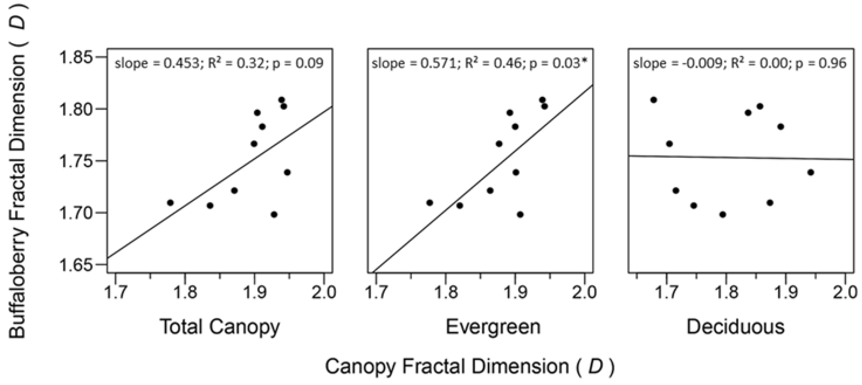
Relationships between fractal dimensions of canopy and buffaloberry were positive for evergreen and total canopy cover (Figure 6). The evergreen canopy and buffaloberry fractal dimensions demonstrated the strongest relationship with the greatest slope (R2 = 0.46; β = 0.571), while the relationship between the total canopy and buffaloberry fractal dimensions was weaker with a shallower slope (R2 = 0.32; β = 0.453). The evergreen canopy fractal dimension significantly predicted the fractal dimension of buffaloberry shrubs (p = 0.03), while the effect of the total canopy fractal dimension was weakly significant (p = 0.09) and no relationship was found between deciduous canopy and buffaloberry fractal dimensions (R2 = 0.00; β = −0.009; p = 0.96).
4. Discussion
Our results indicate that the effect of forest canopy on buffaloberry presence, as well as relationships between canopy and buffaloberry heterogeneity, differ between evergreen and deciduous types based on intercepts measured along 20 km of transects. These findings support our hypothesis regarding the distinct effects of evergreen and deciduous canopy on buffaloberry patterns, and the variability of these through space.
4.1. Effects of Canopy on Buffaloberry Presence across Spatial Scales
The evergreen canopy demonstrated a significant negative effect at the local scale, which suggests that microhabitat light availability could be an important factor for buffaloberry presence given the shade-intolerance of this species and the canopy composition we observed. Variation in light transmission exists within evergreen and deciduous categories [26,28], however, stands comprised of evergreen species common to our study area, including white spruce, may transmit less light than typical deciduous species such as trembling aspen [24,25]. Aspen canopies have been found to transmit 14–40% of incident light, compared to 5–11% for those dominated by white spruce [24], with light transmission decreasing with spruce abundance in mixedwoods [24,25]. Light variability can structure understory shrub patterns at both fine spatial scales [82] and the stand-level [83], with model-based sunlight being an important predictor of buffaloberry shrub presence [84]. Evergreen trees may additionally decrease local soil moisture content, pH, and temperature [16,85,86,87,88] which could reduce buffaloberry growth, therefore suggesting that the overall negative effect of the evergreen canopy on shrub presence may not be fully explained by light availability. These results are consistent with previous work that showed that understory vascular plant cover was negatively associated with the cover of white spruce at scales of 5 m to 15 m, but positively associated with aspen and balsam poplar cover over the same spatial range in a nearby boreal mixedwood forest [23].
We found that the positive effect of deciduous canopy was the strongest and most significant at the meso-scale level, implying that the cumulative effect of multiple deciduous trees is most important for buffaloberry presence. Deciduous trees may promote understory shrub growth by allowing high light penetration during seasonal leaf-off periods [25,89], which is particularly crucial for the reproductive success of buffaloberry shrubs due to their early flowering. Canopy light transmission also increases with the basal area of deciduous trees [24], and thus their influence could be most apparent at broader spatial extents that support more mature individuals, amounting to a stand-type effect. Stands with a greater proportion of deciduous trees also occur more often at low elevations in the study area, which are more favourable for buffaloberry. Site properties that vary with elevation and are not entirely determined by canopy, such as temperature, could also then be partly responsible for the positive spatial relationship with deciduous canopy observed here.
The sharp decline in the strength of the deciduous canopy relationship after ~360 m implies a spatial limit to this meso-scale effect. This decrease could relate to the abundance of evergreen trees in the study area, such that expanding the spatial scale past this point might not incorporate additional deciduous trees, thereby weakening the effect. The effect of evergreen canopy was also low at similar scales, particularly around 300 m and 420 m, which suggests that disturbances from timber harvesting may begin to moderate the influence of the forest canopy as the spatial scale increases. Clear-cutting is the primary harvesting method in the study area, and at scales above 300 m, most transect replicates would have traversed a cutblock at some stage of regeneration (age). Buffaloberry occurred sparsely in cutblocks, but the lack of shrubs here was likely caused by removal during harvesting and their slow growth habit [90], rather than a forest canopy effect. Harvesting also alters the microclimate [91] and edaphic conditions [92], which could contribute to the absence of shrubs in cutblocks if these changes are unfavourable for buffaloberry and impede recolonization. Buffaloberry patch size distribution might be expected to deviate from a power law relationship due to the prevalence of forest harvesting in the area [14], although this was not observed here. As we did not measure shrubs in an undisturbed control forest, we cannot assess whether forest management has altered the abundance of buffaloberry patches of various sizes. Future comparisons of buffaloberry patch size distributions between disturbed and undisturbed stands could offer insight into the effect of harvesting on shrub patterns.
4.2. Relationships between Spatial Heterogeneity of the Forest Canopy and Buffaloberry
Through fractal analysis we found a significant positive relationship between evergreen canopy and buffaloberry fractal dimensions, suggesting that the heterogeneity of evergreen trees scales with the heterogeneity of buffaloberry shrubs. Thus, greater canopy heterogeneity is associated with greater buffaloberry heterogeneity, which supports our hypothesis. This relationship was less significant when total canopy, including deciduous trees, was evaluated.
The stronger correlation of buffaloberry patterns with evergreen canopy heterogeneity may be linked to the dominance of evergreen trees within forests in the study area. Timber harvesting in the area focuses on evergreen species, and thus simultaneous disturbance to overstory and understory strata is more likely in evergreen stands. This may represent a mechanism by which evergreen heterogeneity could promote the heterogeneity of buffaloberry shrubs. Other environmental factors affecting both canopy and buffaloberry spatial patterns may therefore have contributed to our findings, and it is not likely that these are exclusively due to differential regulatory effects of canopy types on understory resources such as light. Mean annual temperature, growing season precipitation, soil texture, and soil pH have been identified as important predictors of buffaloberry presence [84], and presumably also influence the distribution of tree species in the study area. These considerations point to complex linkages between forest overstory and understory heterogeneity.
Heterogeneity can be an ambiguous term in the ecological literature when the definition is not made explicit [2,3,93,94]. Numerous conceptual interpretations and the multitude of ecological characteristics that can be measured result in a variety of data types and analytical techniques for examining environmental heterogeneity. Here we use the fractal measure of D as a heterogeneity metric, the value of which may change with the analysis scale [31,78]; this is not surprising given that it indicates heterogeneity. Quantifying vegetation patterns at a common scale, as we have here, enables comparisons of the relative heterogeneity of plant species [51]. Calculating the fractal dimension as a function of scale can reveal whether vegetation heterogeneity varies in space and can identify hierarchical patterns [31]. Regions where D remains stable constitute domains of scale between which are transitions that may signify shifts in the processes governing heterogeneity [4,6]. These dynamics may be of interest for future research of forest spatial patterns and the mechanisms that shape them.
As different calculation methods can produce different D values for identical data [95], comparing results among fractal studies with distinct methodologies can be misleading. We are not aware of examples from the literature that utilize a box-counting technique with transect data in order to evaluate horizontal heterogeneity of forest vegetation; this has, however, been applied in grassland systems [48]. We found that buffaloberry is less heterogeneous and fractal-like over fewer orders of magnitude than big sagebrush, another woody shrub, as measured in a Utah steppe at a similar 1.6 km transect scale [48]. It is worth noting that, despite methodological differences, forest canopies are usually determined to be quite homogeneous [56,96,97] and fractal-like over several orders of magnitude [43], which is in line with the findings of this study.
The box-counting technique used here relies on sequential binary observations that are a type of one-dimensional point pattern. This is ideal for line-intercept data, such as those which represent vegetation presence along a transect. In contrast, point pattern analyses typically assess the distribution of a material over a two-dimensional plane [98], such as the spatial arrangement of individual trees across a landscape [99,100]. One-dimensional analyses of forest vegetation primarily involve continuous, rather than binary, data and consider heterogeneity in terms of variance as a function of scale [31,78]. Wavelet analysis, for example, is a multi-scale approach [101] that can incorporate remote sensing data to identify hierarchical patterns in horizontal attributes like canopy gap structure [102,103] and tree crown diameter [104,105]. Here the line-intercept sampling of both shrub and canopy layers produced sets of binary data for each of these strata, and enabled direct comparisons of their heterogeneity through the calculation of their respective fractal dimensions.
5. Conclusions
This study highlights the importance of spatial scale and forest canopy composition for characterizing patterns of understory plant presence and relationships between canopy and understory heterogeneity. Fractal analysis addresses issues of scale-dependence associated with the quantification of environmental heterogeneity, but has been mostly overlooked as a tool for examining forest vegetation patterns and spatial relationships. The box-counting approach used with line-intercept transects is a straightforward and practical technique that enables multi-scale assessments of vegetation heterogeneity, represented by a single metric, D, and can identify fractal-like vegetation patterns.
Indicators of heterogeneity and fractal-like properties for key animal resources, like fruiting shrubs [106,107], can contribute to studies of foraging strategy, consumer-resource interactions, and animal movement in spatially complex environments [108,109,110,111,112]. Fractal-like resource distributions, for example, point to scale-dependence in resource density and consumer foraging behaviour as determined by animal body size, which controls the scale of environmental perception [109,110,111] or environmental grain [113]. The significant relationship identified here between evergreen canopy and buffaloberry heterogeneity indicates the potential for estimating understory plant patterns from canopy patterns, which can be measured at broad spatial extents using remote sensing, and could contribute to the quantification of buffaloberry fruit or other wildlife resources at the landscape-level.
Acknowledgments
We received funding for this research from the Natural Sciences and Engineering Research Council of Canada (NSERC) and the Alberta Conservation Association (ACA), as well as in-kind support from fRI Research. Thank you to N. Kenkel and M.E. Ritchie for insights into box-counting methodology, to the Integrated Remote Sensing Studio (IRSS) at the University of British Columbia (UBC) for providing processed LiDAR data for stratification of field transects, and to K. Mulligan for assistance with fieldwork.
Author Contributions
Catherine Denny and Scott Nielsen jointly developed the study design. Catherine Denny collected the field data, performed the analyses, and wrote the manuscript with assistance from Scott Nielsen.
Conflicts of Interest
The authors declare no conflict of interest. The funding agency had no role in the design of the study; in the collection, analyses, or interpretation of data; or in the preparation of the manuscript.
References
- Urban, D.L.; O’Neill, R.V.; Shugart, H.H. Landscape ecology. Bioscience 1987, 37, 119–127. [Google Scholar] [CrossRef]
- Kolasa, J.; Rollo, C.D. Introduction: The heterogeneity of heterogeneity: A glossary. In Ecological Heterogeneity; Kolasa, J., Pickett, S.T.A., Eds.; Springer: New York, NY, USA, 1991; pp. 1–23. [Google Scholar]
- Li, H.; Reynolds, J.F. On definition and quantification of heterogeneity. Oikos 1995, 73, 280–284. [Google Scholar] [CrossRef]
- Wiens, J.A. Spatial scaling in ecology. Funct. Ecol. 1989, 3, 385–397. [Google Scholar] [CrossRef]
- Levin, S.A. The problem of pattern and scale in ecology. Ecology 1992, 73, 1943–1967. [Google Scholar] [CrossRef]
- Mandelbrot, B.B. The Fractal Geometry of Nature; W.H. Freeman and Company: New York, NY, USA, 1982. [Google Scholar]
- Allen, T.F.H.; Hoekstra, T.W. Toward a Unified Ecology; Columbia University Press: New York, NY, USA, 1992. [Google Scholar]
- Kotliar, N.B.; Wiens, J.A. Multiple scales of patchiness and patch structure: A hierarchical framework for the study of heterogeneity. Oikos 1990, 59, 253–260. [Google Scholar] [CrossRef]
- Watt, A.S. Pattern and process in the plant community. J. Ecol. 1947, 35, 1–22. [Google Scholar] [CrossRef]
- Whittaker, R.H. The design and stability of plant communities. In Unifying Concepts in Ecology; van Dobben, W.H., Lowe-McConnell, R.H., Eds.; Dr. W. Junk B.V. Publishers: The Hague, The Netherlands, 1975; pp. 169–183. [Google Scholar]
- Levin, S.A. Pattern formation in ecological communities. In Spatial Pattern in Plankton Communities; Steele, J.H., Ed.; Plenum Press: New York, NY, USA, 1978; pp. 433–465. [Google Scholar]
- Sousa, W.P. The role of disturbance in natural communities. Annu. Rev. Ecol. Syst. 1984, 15, 353–391. [Google Scholar] [CrossRef]
- Franklin, J.F.; Forman, R.T.T. Creating landscape patterns by forest cutting: Ecological consequences and principles. Landsc. Ecol. 1987, 1, 5–18. [Google Scholar] [CrossRef]
- Kéfi, S.; Rietkerk, M.; Alados, C.L.; Pueyo, Y.; Papanastasis, V.P.; Elaich, A.; de Ruiter, P.C. Spatial vegetation patterns and imminent desertification in Mediterranean arid ecosystems. Nature 2007, 449, 213–217. [Google Scholar] [CrossRef] [PubMed]
- Jennings, S.B.; Brown, N.D.; Sheil, D. Assessing forest canopies and understorey illumination: Canopy closure, canopy cover and other measures. Forestry 1999, 72, 59–74. [Google Scholar] [CrossRef]
- Beatty, S.W. Influence of microtopography and canopy species on spatial patterns of forest understory plants. Ecology 1984, 65, 1406–1419. [Google Scholar] [CrossRef]
- Boettcher, S.E.; Kalisz, P.J. Single-tree influence on soil properties in the mountains of eastern Kentucky. Ecology 1990, 71, 1365–1372. [Google Scholar] [CrossRef]
- Russell, E.W. Soil Conditions and Plant. Growth, 9th ed.; Longmans: London, UK, 1961. [Google Scholar]
- Smith, H. Light quality, photoperception, and plant strategy. Annu. Rev. Plant Physiol. 1982, 33, 481–518. [Google Scholar] [CrossRef]
- Bartels, S.F.; Chen, H.Y.H. Is understory plant species diversity driven by resource quantity or resource heterogeneity? Ecology 2010, 91, 1931–1938. [Google Scholar] [CrossRef] [PubMed]
- Macdonald, S.E.; Fenniak, T.E. Understory plant communities of boreal mixedwood forests in western Canada: Natural patterns and response to variable-retention harvesting. For. Ecol. Manag. 2007, 242, 34–48. [Google Scholar] [CrossRef]
- Pelletier, B.; Fyles, J.W.; Dutilleul, P. Tree species control and spatial structure of forest floor properties in a mixed-species stand. Ecoscience 1999, 6, 79–91. [Google Scholar]
- Kembel, S.W.; Dale, M.R.T. Within-stand spatial structure and relation of boreal canopy and understorey vegetation. J. Veg. Sci. 2006, 17, 783–790. [Google Scholar] [CrossRef]
- Lieffers, V.J.; Stadt, K.J. Growth of understory Picea. glauca, Calamagrostis. canadensis, and Epilobium. angustifolium in relation to overstory light transmission. Can. J. For. Res. 1994, 24, 1193–1198. [Google Scholar] [CrossRef]
- Constabel, A.J.; Lieffers, V.J. Seasonal patterns of light transmission through boreal mixedwood canopies. Can. J. For. Res. 1996, 26, 1008–1014. [Google Scholar] [CrossRef]
- Canham, C.D.; Finzi, A.C.; Pacala, S.W.; Burbank, D.H. Causes and consequences of resource heterogeneity in forests: Interspecific variation in light transmission by canopy trees. Can. J. For. Res. 1994, 24, 337–349. [Google Scholar] [CrossRef]
- Chen, H.Y.H.; Klinka, K.; Kayahara, G.J. Effects of light on growth, crown architecture, and specific leaf area for naturally established Pinus. contorta var. latifolia and Pseudotsuga. menziesii var. glauca saplings. Can. J. For. Res. 1996, 26, 1149–1157. [Google Scholar]
- Messier, C.; Parent, S.; Bergeron, Y. Characterization of understory light environment in closed mixed boreal forests: Effects of overstory and understory vegetation. J. Veg. Sci. 1998, 9, 511–520. [Google Scholar] [CrossRef]
- Lieffers, V.J.; Pinno, B.D.; Stadt, K.J. Light dynamics and free-to-grow standards in aspen-dominated mixedwood forests. For. Chron. 2002, 78, 137–145. [Google Scholar] [CrossRef]
- Lieffers, V.J.; Messier, C.; Stadt, K.J.; Gendron, F.; Comeau, P.G. Predicting and managing light in the understory of boreal forests. Can. J. For. Res. 1999, 29, 796–811. [Google Scholar] [CrossRef]
- Palmer, M.W. Fractal geometry: A tool for describing spatial patterns of plant communities. Vegetatio 1988, 75, 91–102. [Google Scholar] [CrossRef]
- Spies, T.A.; Franklin, J.F. Gap characteristics and vegetation response in coniferous forests of the Pacific Northwest. Ecology 1989, 70, 543–545. [Google Scholar] [CrossRef]
- Klinka, K.; Chen, H.Y.H.; Wang, Q.; de Montigny, L. Forest canopies and their influence on understory vegetation in early-seral stands on West Vancouver Island. Northwest Sci. 1996, 70, 193–200. [Google Scholar]
- Berger, A.L.; Puettmann, K.J. Overstory composition and stand structure influence herbaceous plant diversity in the mixed aspen forest of northern Minnesota. Am. Midl. Nat. 2000, 143, 111–125. [Google Scholar] [CrossRef]
- Svenning, J.-C.; Skov, F. Mesoscale distribution of understorey plants in temperate forest (Kalø, Denmark): The importance of environment and dispersal. Plant Ecol. 2002, 160, 169–185. [Google Scholar] [CrossRef]
- Tewksbury, J.J.; Lloyd, J.D. Positive interactions under nurse-plants: Spatial scale, stress gradients and benefactor size. Oecologia 2001, 127, 425–434. [Google Scholar] [CrossRef]
- Allen, T.F.H.; Starr, T.B. Hierarchy: Perspectives for Ecological Complexity; University of Chicago Press: Chicago, IL, USA, 1982. [Google Scholar]
- Li, B.-L. Fractal geometry applications in description and analysis of patch patterns and patch dynamics. Ecol. Model. 2000, 132, 33–50. [Google Scholar] [CrossRef]
- Brosofske, K.D.; Chen, J.; Crow, T.R.; Saunders, S.C. Vegetation responses to landscape structure at multiple scales across a Northern Wisconsin, USA, pine barrens landscape. Plant Ecol. 1999, 143, 203–218. [Google Scholar] [CrossRef]
- Burrough, P.A. Fractal dimensions of landscapes and other environmental data. Nature 1981, 294, 240–242. [Google Scholar] [CrossRef]
- Frontier, S. Applications of fractal theory to ecology. In Developments in Numerical Ecology; Legendre, P., Legendre, L., Eds.; Springer: Berlin/Heidelberg, Germany, 1987; pp. 335–378. [Google Scholar]
- Milne, B.T. Spatial aggregation and neutral models in fractal landscapes. Am. Nat. 1992, 139, 32–57. [Google Scholar] [CrossRef]
- Milne, B.T. Applications of fractal geometry in wildlife biology. In Wildlife and Landscape Ecology: Effects of Pattern and Scale; Bissonette, J.A., Ed.; Springer: New York, NY, USA, 1997; pp. 32–69. [Google Scholar]
- Brown, J.H.; Gupta, V.K.; Li, B.-L.; Milne, B.T.; Restrepo, C.; West, G.B. The fractal nature of nature: Power laws, ecological complexity and biodiversity. Philos. Trans. R. Soc. B 2002, 357, 619–626. [Google Scholar] [CrossRef] [PubMed]
- Barnsley, M.F. Fractals Everywhere; Academic Press: San Diego, CA, USA, 1988. [Google Scholar]
- Milne, B.T. Lessons from applying fractal models to landscape patterns. In Quantitative Methods in Landscape Ecology; Turner, M.G., Gardner, R.H., Eds.; Springer: New York, NY, USA, 1991; pp. 199–235. [Google Scholar]
- Voss, R.F. Characterization and measurement of random fractals. Phys. Scr. 1986, T13, 27–32. [Google Scholar] [CrossRef]
- Ritchie, M.E.; Wolfe, M.L.; Danvir, R. Predation of artificial sage grouse nests in treated and untreated sagebrush. Gr. Basin Nat. 1994, 54, 122–129. [Google Scholar]
- Ritchie, M.E. Scale, Heterogeneity, and the Structure and Diversity of Ecological Communities; Princeton University Press: Princeton, NJ, USA, 2010. [Google Scholar]
- Olff, H.; Ritchie, M.E. Fragmented nature: Consequences for biodiversity. Landsc. Urban Plan. 2002, 58, 83–92. [Google Scholar] [CrossRef]
- Kenkel, N.C.; Walker, D.J. Fractals in the biological sciences. Coenoses 1996, 11, 77–100. [Google Scholar]
- Krummel, J.R.; Gardner, R.H.; Sugihara, G.; O’Neill, R.V.; Coleman, P.R. Landscape patterns in a disturbed environment. Oikos 1987, 48, 321–324. [Google Scholar] [CrossRef]
- Rex, K.D.; Malanson, G.P. The fractal shape of riparian forest patches. Landsc. Ecol. 1990, 4, 249–258. [Google Scholar] [CrossRef]
- Mladenoff, D.J.; White, M.A.; Pastor, J.; Crow, T.R. Comparing spatial pattern in unaltered old-growth and disturbed forest landscapes. Ecol. Appl. 1993, 3, 294–306. [Google Scholar] [CrossRef] [PubMed]
- Drake, J.B.; Weishampel, J.F. Multifractal analysis of canopy height measures in a longleaf pine savanna. For. Ecol. Manag. 2000, 128, 121–127. [Google Scholar] [CrossRef]
- Parker, G.G.; Russ, M.E. The canopy surface and stand development: Assessing forest canopy structure and complexity with near-surface altimetry. For. Ecol. Manag. 2004, 189, 307–315. [Google Scholar] [CrossRef]
- Morse, D.R.; Lawton, J.H.; Dodson, M.M.; Williamson, M.H. Fractal distribution of vegetation and the distribution of arthropod body lengths. Nature 1985, 314, 731–733. [Google Scholar] [CrossRef]
- Gunnarsson, B. Fractal dimension of plants and body size distribution in spiders. Funct. Ecol. 1992, 6, 636–641. [Google Scholar] [CrossRef]
- Escós, J.; Alados, C.L.; Emlen, J.M. The impact of grazing on plant fractal architecture and fitness of a Mediterranean shrub Anthyllis. cytisoides L. Funct. Ecol. 1997, 11, 66–78. [Google Scholar] [CrossRef]
- Alados, C.L.; Emlen, J.M.; Wachocki, B.; Freeman, D.C. Instability of development and fractal architecture in dryland plants as an index of grazing pressure. J. Arid Environ. 1998, 38, 63–76. [Google Scholar] [CrossRef]
- Humbert, L.; Gagnon, D.; Kneeshaw, D.; Messier, C. A shade tolerance index for common understory species of northeastern North America. Ecol. Indic. 2007, 7, 195–207. [Google Scholar] [CrossRef]
- Stringer, P.W.; La Roi, G.H. The Douglas-fir forests of Banff and Jasper National Parks, Canada. Can. J. Bot. 1970, 48, 1703–1726. [Google Scholar] [CrossRef]
- La Roi, G.H.; Hnatiuk, R.J. The Pinus. contorta forests of Banff and Jasper National Parks: A study in comparative synecology and syntaxonomy. Ecol. Monogr. 1980, 50, 1–29. [Google Scholar] [CrossRef]
- Moss, E.H. Flora of Alberta, 2nd ed.; University of Toronto Press: Toronto, ON, Canada, 1983. [Google Scholar]
- Johnson, K.; Nielsen, S.E. Demographic effects on fruit set in the dioecious shrub Canada buffaloberry (Shepherdia. canadensis). PeerJ 2014, 2, e526. [Google Scholar] [CrossRef] [PubMed]
- Hamer, D. Buffaloberry (Shepherdia. canadensis (L.) Nutt.) fruit production in fire-successional bear feeding sites. J. Range Manag. 1996, 49, 520–529. [Google Scholar] [CrossRef]
- Nielsen, S.E.; Munro, R.H.M.; Bainbridge, E.L.; Stenhouse, G.B.; Boyce, M.S. Grizzly bears and forestry II. distribution of grizzly bear foods in clearcuts of west-central Alberta, Canada. For. Ecol. Manag. 2004, 199, 67–82. [Google Scholar] [CrossRef]
- Achuff, P.L. Natural Regions, Subregions and Natural History Themes of Alberta: A Classification for Protected Areas Management; Alberta Environmental Protection: Edmonton, AB, Canada, 1994. [Google Scholar]
- Udell, R.; Murphy, P.J.; Renaud, D. A 50-Year History of Silviculture on the Hinton Forest 1955–2005: Adaptive Management in Practice; Foothills Research Institute: Hinton, AB, Canada, 2013. [Google Scholar]
- Coops, N.C.; Tompaski, P.; Nijland, W.; Rickbeil, G.J.M.; Nielsen, S.E.; Bater, C.W.; Stadt, J.J. A forest structure habitat index based on airborne laser scanning data. Ecol. Indic. 2016, 67, 346–357. [Google Scholar] [CrossRef]
- ESRI. ArcGIS Desktop: ArcMap Version 10.2.1; Environmental Systems Research Institute: Redlands, CA, USA, 2014. [Google Scholar]
- R Development Core Team. R: A Language and Environment for Statistical Computing, 3.1.2; R Foundation for Statistical Computing: Vienna, Austria, 2014. [Google Scholar]
- Huang, S.; Titus, S.J.; Wiens, D.D. Comparison of nonlinear height-diameter functions for major Alberta tree species. Can. J. For. Res. 1992, 22, 1297–1304. [Google Scholar] [CrossRef]
- Clark, D.B.; Palmer, M.W.; Clark, D.A. Edaphic factors and the landscape-scale distributions of tropical rain forest trees. Ecology 1998, 80, 2662–2675. [Google Scholar] [CrossRef]
- Bates, D.; Mächler, M.; Bolker, B.M.; Walker, S.C. Fitting linear mixed-effects models using lme4. J. Stat. Softw. 2015, 67, 1–48. [Google Scholar] [CrossRef]
- Akaike, H. A new look at the statistical model identification. IEEE Trans. Autom. Control 1974, 19, 716–723. [Google Scholar] [CrossRef]
- Burnham, K.P.; Anderson, D.R. Model. Selection and Inference, 2nd ed.; Springer: New York, NY, USA, 2002. [Google Scholar]
- Leduc, A.; Prairie, Y.T.; Bergeron, Y. Fractal dimension estimates of a fragmented landscape: Sources of variability. Landsc. Ecol. 1994, 9, 279–286. [Google Scholar] [CrossRef]
- Taylor, C.C.; Taylor, S.J. Estimating the dimension of a fractal. J. R. Stat. Soc. Ser. B Stat. Methodol. 1991, 53, 353–364. [Google Scholar]
- Halley, J.M.; Hartley, S.; Kallimanis, A.S.; Kunin, W.E.; Lennon, J.J.; Sgardelis, S.P. Uses and abuses of fractal methodology in ecology. Ecol. Lett. 2004, 7, 254–271. [Google Scholar] [CrossRef]
- Kenkel, N.C. Sample size requirements for fractal dimension estimation. Community Ecol. 2013, 14, 144–152. [Google Scholar] [CrossRef]
- Frelich, L.E.; Machado, J.-L.; Reich, P.B. Fine-scale environmental variation and structure of understorey plant communities in two old-growth pine forests. J. Ecol. 2003, 91, 283–293. [Google Scholar] [CrossRef]
- Reich, P.B.; Frelich, L.E.; Voldseth, R.A.; Bakken, P.; Adair, E.C. Understorey diversity in southern boreal forests is regulated by productivity and its indirect impacts on resource availability and heterogeneity. J. Ecol. 2012, 100, 539–545. [Google Scholar] [CrossRef]
- Nielsen, S.E.; Larsen, T.A.; Stenhouse, G.B.; Coogan, S.C.P. Complementary food resources of carnivory and frugivory affect local abundance of an omnivorous carnivore. Oikos 2017, 126, 369–380. [Google Scholar] [CrossRef]
- Nihlgård, B. Pedological influence of spruce planted on former beech forest soils in Scania, south Sweden. Oikos 1971, 22, 302–314. [Google Scholar] [CrossRef]
- Binkley, D.; Valentine, D. Fifty-year biogeochemical effects of green ash, white pine, and Norway spruce in a replicated experiment. For. Ecol. Manag. 1991, 40, 13–25. [Google Scholar] [CrossRef]
- Ste-Marie, C.; Paré, D. Soil, pH and N availability effects on net nitrification in the forest floors of a range of boreal forest stands. Soil Biol. Biochem. 1999, 31, 1579–1589. [Google Scholar] [CrossRef]
- Hobbie, S.E.; Reich, P.B.; Oleksyn, J.; Ogdahl, M.; Zytkowiak, R.; Hale, C.; Karolewski, P. Tree species effects on decomposition and forest floor dynamics in a common garden. Ecology 2006, 87, 2288–2297. [Google Scholar] [CrossRef]
- Ross, M.S.; Flanagan, L.B.; La Roi, G.H. Seasonal and successional changes in light quality and quantity in the understory of boreal forest ecosystems. Can. J. Bot. 1986, 64, 2792–2799. [Google Scholar] [CrossRef]
- Densmore, R.V.; Vander Meer, M.E.; Dunkle, N.G. Native Plant Revegetation Manual for Denali National Park and Preserve; Information and Technology Report USGS/BRD/ITR-2000-0006; US Geological Survey: Anchorage, AK, USA, 2000.
- Chen, J.; Franklin, J.F.; Spies, T.A. Contrasting microclimates among clearcut, edge, and interior of old-growth Douglas-fir forest. Agric. For. Meteorol. 1993, 63, 219–237. [Google Scholar] [CrossRef]
- Pennock, D.J.; van Kessel, C. Clear-cut forest harvest impacts on soil quality indicators in the mixedwood forest of Saskatchewan, Canada. Geoderma 1997, 75, 13–32. [Google Scholar] [CrossRef]
- Dutilleul, P.; Legendre, P. Spatial heterogeneity against heteroscedasticity: An ecological paradigm versus a statistical concept. Oikos 1993, 66, 152–171. [Google Scholar] [CrossRef]
- Li, H.; Reynolds, J.F. A simulation experiment to quantify spatial heterogeneity in categorical maps. Ecology 1994, 75, 2446–2455. [Google Scholar] [CrossRef]
- Malinverno, A. Testing linear models of sea-floor topography. Pure Appl. Geophys. 1989, 131, 139–155. [Google Scholar] [CrossRef]
- Weishampel, J.F.; Blair, J.B.; Dubayah, R.; Clark, D.B.; Knox, R.G. Canopy topography of an old-growth tropical rain forest landscape. Selbyana 2000, 21, 79–87. [Google Scholar]
- Boutet, J.C.; Weishampel, J.F. Spatial pattern analysis of pre- and post-hurricane forest canopy structure in North Carolina, USA. Landsc. Ecol. 2003, 18, 553–559. [Google Scholar] [CrossRef]
- Wiegand, T.; Moloney, K.A. Handbook of Spatial Point-Pattern Analysis in Ecology; Chapman and Hall/CRC Press: Boca Raton, FL, USA, 2014. [Google Scholar]
- Moeur, M. Characterizing spatial patterns of trees using stem-mapped data. For. Sci. 1993, 39, 756–775. [Google Scholar]
- He, F.; Legendre, P.; LaFrankie, J.V. Distribution patterns of tree species in a Malaysian tropical rain forest. J. Veg. Sci. 1997, 8, 105–114. [Google Scholar]
- Daubechies, I. Othornormal bases of compactly supported wavelets. Commun. Pure Appl. Math. 1988, 41, 909–996. [Google Scholar] [CrossRef]
- Bradshaw, G.A.; Spies, T.A. Characterizing canopy gap structure in forests using wavelet analysis. J. Ecol. 1992, 80, 205–215. [Google Scholar] [CrossRef]
- Kane, V.R.; Gersonde, R.F.; Lutz, J.A.; McGaughey, R.J.; Bakker, J.D.; Franklin, J.F. Patch dynamics and the development of structural and spatial heterogeneity in Pacific Northwest forests. Can. J. For. Res. 2011, 41, 2276–2291. [Google Scholar] [CrossRef]
- Falkowski, M.J.; Smith, A.M.S.; Hudak, A.T.; Gessler, P.E.; Vierling, L.A.; Crookston, N.L. Automated estimation of individual conifer tree height and crown diameter via two-dimensional spatial wavelet analysis of lidar data. Can. J. Remote Sens. 2006, 32, 153–161. [Google Scholar] [CrossRef]
- Strand, E.K.; Smith, A.M.S.; Bunting, S.C.; Vierling, L.A.; Hann, D.B.; Gessler, P.E. Wavelet estimation of plant spatial patterns in multitemporal aerial photography. Int. J. Remote Sens. 2006, 27, 2049–2054. [Google Scholar] [CrossRef]
- McLellan, B.N.; Hovey, F.W. The diet of grizzly bears in the Flathead River drainage of southeastern British Columbia. Can. J. Zool. 1995, 73, 704–712. [Google Scholar] [CrossRef]
- Munro, R.H.M.; Nielsen, S.E.; Price, M.H.; Stenhouse, G.B.; Boyce, M.S. Seasonal and diel patterns of grizzly bear diet and activity in west-central Alberta. J. Mammal. 2006, 87, 1112–1121. [Google Scholar] [CrossRef]
- Wiens, J.A.; Milne, B.T. Scaling of “landscapes” in landscape ecology, or, landscape ecology from a beetle’s perspective. Landsc. Ecol. 1989, 3, 87–96. [Google Scholar] [CrossRef]
- Ritchie, M.E. Scale-dependent foraging and patch choice in fractal environments. Evol. Ecol. 1998, 12, 309–330. [Google Scholar] [CrossRef]
- Ritchie, M.E.; Olff, H. Spatial scaling laws yield a synthetic theory of biodiversity. Nature 1999, 400, 557–560. [Google Scholar] [CrossRef] [PubMed]
- Haskell, J.P.; Ritchie, M.E.; Olff, H. Fractal geometry predicts varying body size scaling relationships for mammal and bird home ranges. Nature 2002, 418, 527–530. [Google Scholar] [CrossRef] [PubMed]
- Sims, D.W.; Southall, E.J.; Humphries, N.E.; Hays, G.C.; Bradshaw, C.J.A.; Pitchford, J.W.; James, A.; Ahmed, M.Z.; Brierley, A.S.; Hindell, M.A.; et al. Scaling laws of marine predator search behaviour. Nature 2008, 451, 1098–1102. [Google Scholar] [CrossRef] [PubMed]
- Levins, R. Evolution in Changing Environments: Some Theoretical Explorations; Princeton University Press: Princeton, NJ, USA, 1968. [Google Scholar]
Figure 1.
Location and elevation of 2-km transects (n = 10) established in 2015 across the study area southeast of Hinton, Alberta (53°24′41″ N, 117°33′50″ W).
Figure 1.
Location and elevation of 2-km transects (n = 10) established in 2015 across the study area southeast of Hinton, Alberta (53°24′41″ N, 117°33′50″ W).
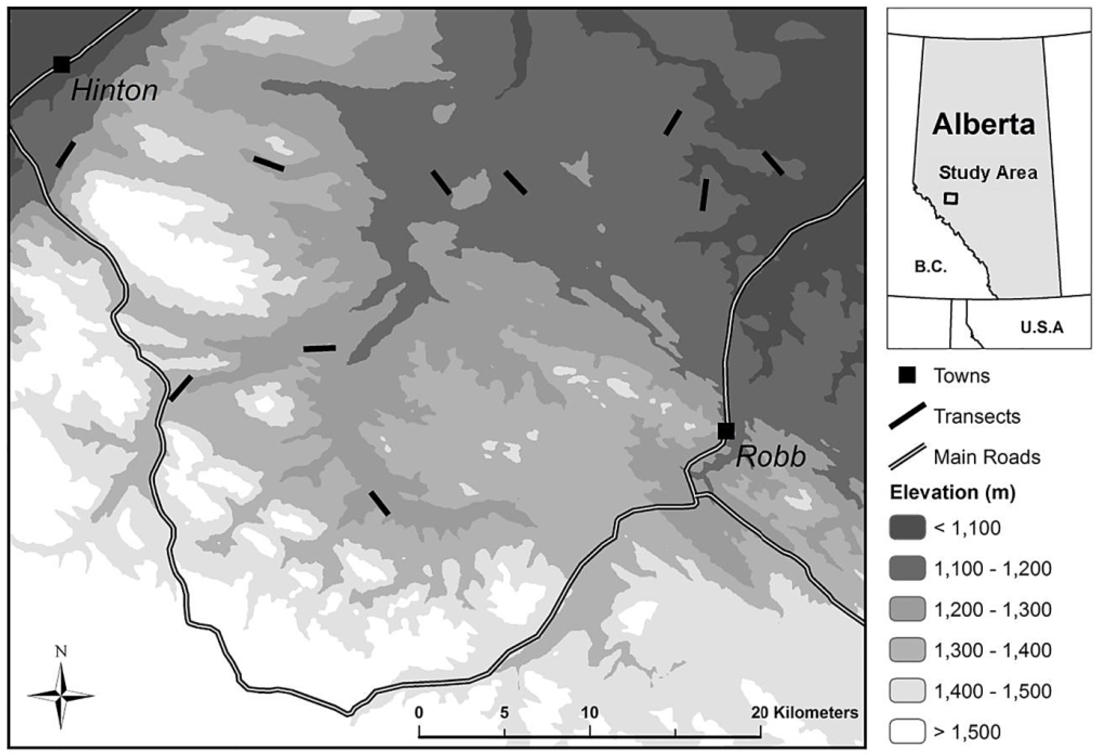
Figure 2.
(a) Frequency distribution of buffaloberry shrub patch sizes (m) among transects based on line-intercept sampling; and (b) the log 10-transformed frequency distribution of buffaloberry patch sizes, where midpoints of each size range were used to calculate transformed values (R2 = 0.88; β = −1.269; p < 0.001).
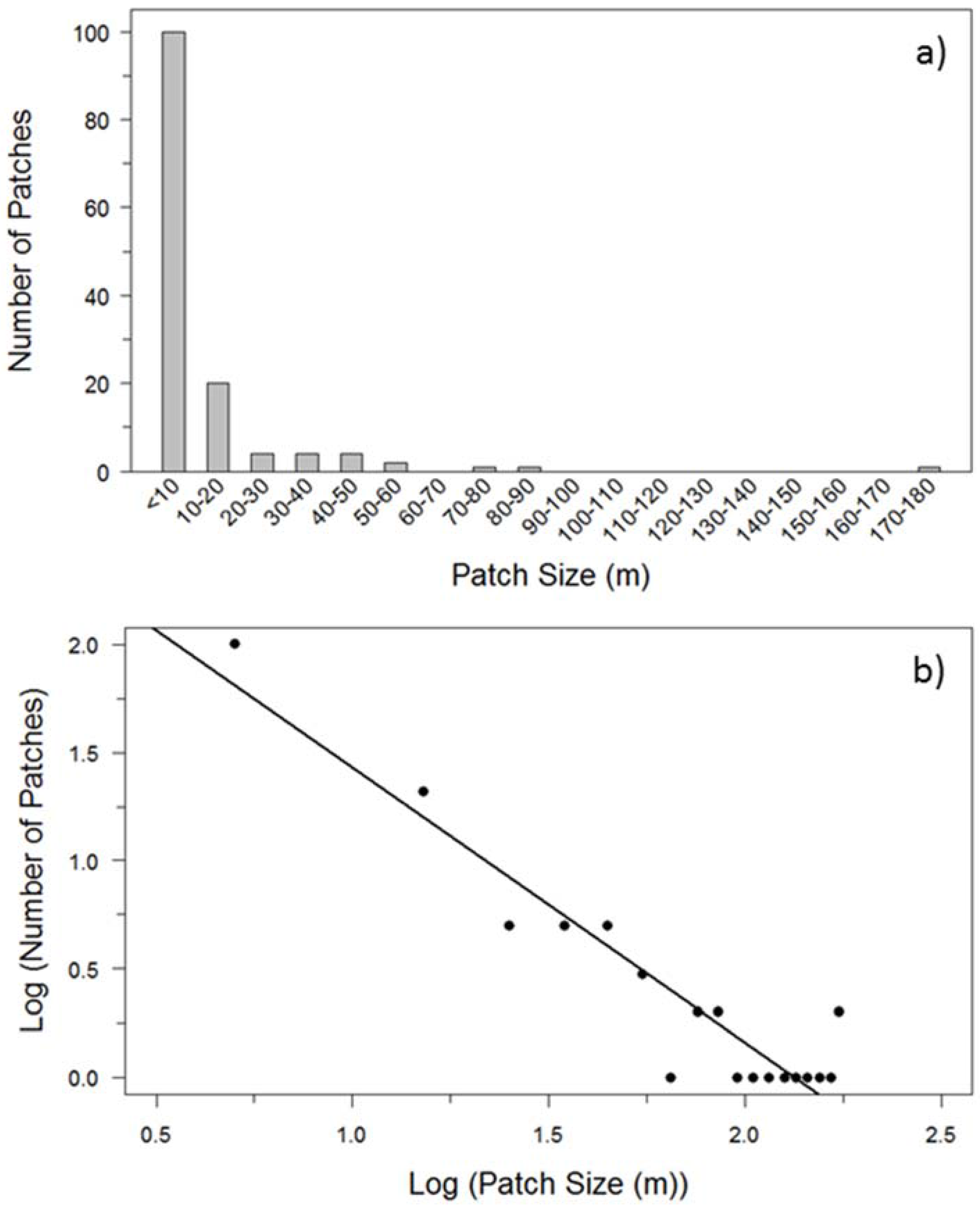
Figure 3.
Example of raw forest canopy (upper bar) and buffaloberry shrub (lower bar) line-intercept transect data for two 2-km replicates (n = 10) representative of (a) average patch size and distribution; and (b) maximum cover of canopy and buffaloberry recorded during field sampling near Hinton, Alberta. The overlap refers to the presence of both evergreen and deciduous canopy within a given segment along a transect.
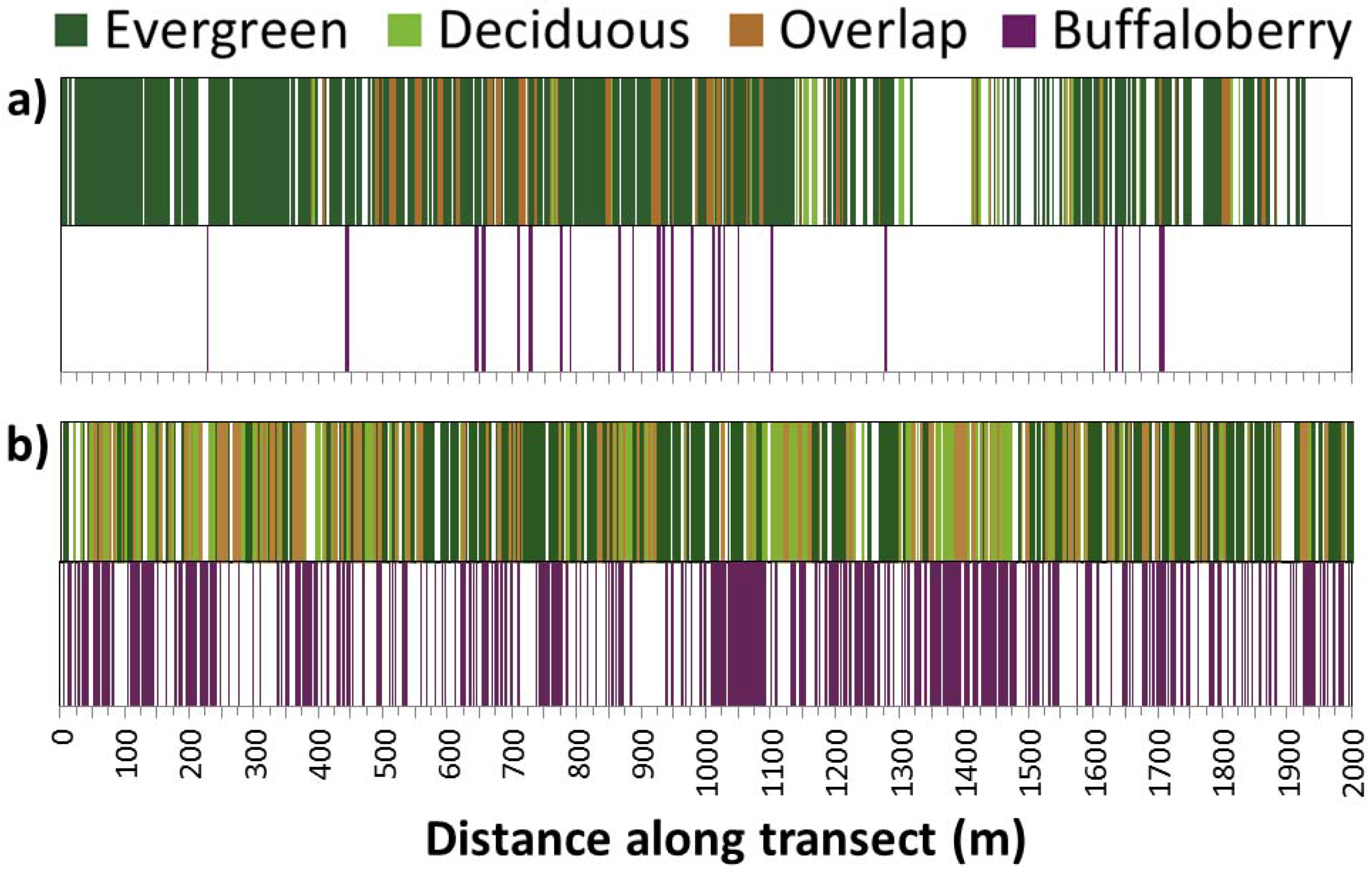
Figure 4.
Effects of total, evergreen, and deciduous canopy cover on buffaloberry shrub presence across spatial scales from 2 m to 502 m, represented as beta (β) coefficients of mixed-effects logistic regression models. Bold lines indicate a significant effect (α = 0.05) at that scale.
Figure 4.
Effects of total, evergreen, and deciduous canopy cover on buffaloberry shrub presence across spatial scales from 2 m to 502 m, represented as beta (β) coefficients of mixed-effects logistic regression models. Bold lines indicate a significant effect (α = 0.05) at that scale.

Figure 5.
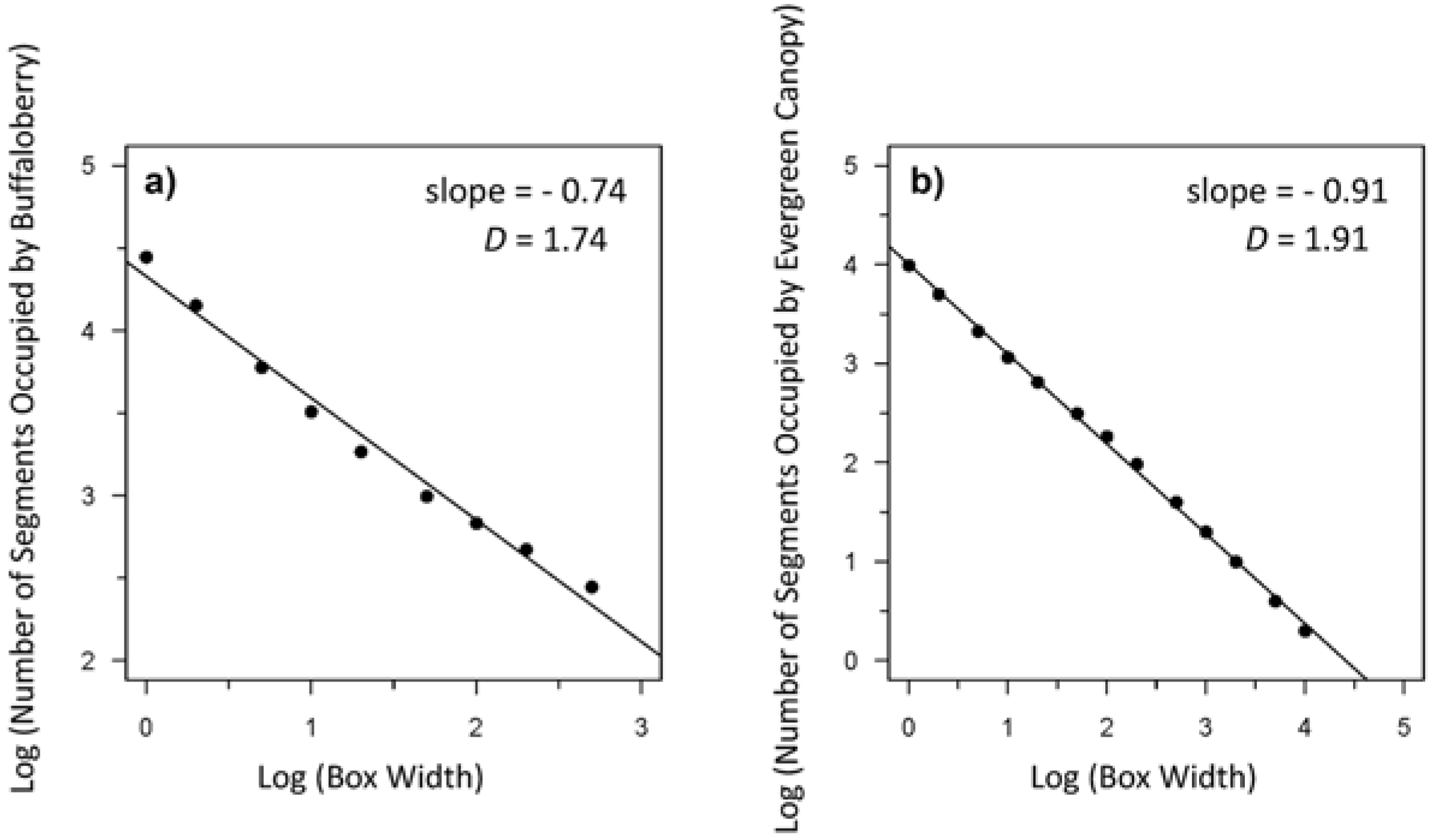
Example from Transect 1 of a log-log plot of the relationship between box width (scale) and the number of segments occupied by (a) buffaloberry (slope = −0.74); and (b) evergreen canopy (slope = −0.91) used to calculate the fractal dimension (D) of each. The slope of the regression line equals 1-D [47] for a given transect. The number of orders of magnitude across which the relationship is fractal-like can be determined based on the x-intercept.
Figure 5.
Example from Transect 1 of a log-log plot of the relationship between box width (scale) and the number of segments occupied by (a) buffaloberry (slope = −0.74); and (b) evergreen canopy (slope = −0.91) used to calculate the fractal dimension (D) of each. The slope of the regression line equals 1-D [47] for a given transect. The number of orders of magnitude across which the relationship is fractal-like can be determined based on the x-intercept.

Figure 6.
General linear models describing relationships between fractal dimensions of buffaloberry shrubs and forest canopy categories. Asterisks indicate a significant effect (α = 0.05). 95% confidence intervals for coefficient estimates of total canopy, evergreen, and deciduous categories were (−0.091, 0.996), (0.064, 1.078), and (−0.401, 0.383), respectively.

Table 1.
Number and width (m) of box-counting segments used for fractal dimension calculations for buffaloberry shrubs and forest canopy.
Table 1.
Number and width (m) of box-counting segments used for fractal dimension calculations for buffaloberry shrubs and forest canopy.
| Intercept Type | Range of Segment or “Box“ Widths (m) | Total Number of Scales |
|---|---|---|
| Buffaloberry | 0.01, 0.02, 0.05, 0.1, 0.2, 0.5, 1, 2, 5 | 9 |
| Total Canopy | 0.1, 0.2, 0.5, 1, 2, 5, 10, 20, 50, 100, 200, 500, 1000 | 13 |
| Evergreen Canopy | 0.1, 0.2, 0.5, 1, 2, 5, 10, 20, 50, 100, 200, 500, 1000 | 13 |
| Deciduous Canopy | 0.1, 0.2, 0.5 | 3 |
Table 2.
Percentage of each transect covered by total, evergreen, and deciduous canopy, as well as buffaloberry shrub intercepts.
Table 2.
Percentage of each transect covered by total, evergreen, and deciduous canopy, as well as buffaloberry shrub intercepts.
| Transect | Total | Evergreen | Deciduous | Buffaloberry |
|---|---|---|---|---|
| Number | Canopy (%) | Canopy (%) | Canopy (%) | Shrubs (%) |
| 1 | 69.0 | 49.4 | 32.5 | 14.0 |
| 2 | 26.8 | 24.2 | 3.4 | 0.1 |
| 3 | 35.8 | 34.1 | 2.7 | 0.5 |
| 4 | 57.7 | 49.0 | 13.7 | 0.9 |
| 5 | 46.0 | 41.8 | 5.4 | 0.2 |
| 6 | 43.4 | 37.2 | 9.0 | 0.2 |
| 7 | 51.0 | 46.7 | 8.3 | 2.0 |
| 8 | 59.4 | 59.4 | 0.0 | 0.4 |
| 9 | 62.3 | 62.2 | 0.1 | 1.3 |
| 10 | 18.5 | 18.1 | 0.6 | 0.3 |
| Mean | 47.0 | 42.2 | 7.6 | 2.0 |
Table 3.
Fractal dimensions of buffaloberry shrubs and forest canopy categories for each transect.
| Transect Number | Total Canopy | Evergreen Canopy | Deciduous Canopy | Buffaloberry Shrubs |
|---|---|---|---|---|
| 1 | 1.95 | 1.91 | 1.95 | 1.74 |
| 2 | 1.84 | 1.83 | 1.75 | 1.71 |
| 3 | 1.88 | 1.87 | 1.72 | 1.72 |
| 4 | 1.94 | 1.91 | 1.80 | 1.70 |
| 5 | 1.91 | 1.90 | 1.84 | 1.80 |
| 6 | 1.91 | 1.88 | 1.71 | 1.77 |
| 7 | 1.92 | 1.91 | 1.90 | 1.78 |
| 8 | 1.95 | 1.95 | 1.69 | 1.81 |
| 9 | 1.95 | 1.95 | 1.86 | 1.80 |
| 10 | 1.79 | 1.78 | 1.88 | 1.71 |
| Mean | 1.90 | 1.89 | 1.81 | 1.75 |
| Minimum | 1.79 | 1.78 | 1.69 | 1.70 |
| Maximum | 1.95 | 1.95 | 1.95 | 1.81 |
| Standard Error | 0.02 | 0.02 | 0.03 | 0.01 |
| 95% Confidence Interval | 1.87, 1.94 | 1.86, 1.92 | 1.76, 1.87 | 1.73, 1.78 |
© 2017 by the authors. Licensee MDPI, Basel, Switzerland. This article is an open access article distributed under the terms and conditions of the Creative Commons Attribution (CC BY) license (http://creativecommons.org/licenses/by/4.0/).
Share and Cite
MDPI and ACS Style
Denny, C.K.; Nielsen, S.E. Spatial Heterogeneity of the Forest Canopy Scales with the Heterogeneity of an Understory Shrub Based on Fractal Analysis. Forests 2017, 8, 146. https://doi.org/10.3390/f8050146
AMA Style
Denny CK, Nielsen SE. Spatial Heterogeneity of the Forest Canopy Scales with the Heterogeneity of an Understory Shrub Based on Fractal Analysis. Forests. 2017; 8(5):146. https://doi.org/10.3390/f8050146
Chicago/Turabian StyleDenny, Catherine K., and Scott E. Nielsen. 2017. "Spatial Heterogeneity of the Forest Canopy Scales with the Heterogeneity of an Understory Shrub Based on Fractal Analysis" Forests 8, no. 5: 146. https://doi.org/10.3390/f8050146
Note that from the first issue of 2016, this journal uses article numbers instead of page numbers. See further details here.