
Introducing a Non-Stationary Matrix Model for Stand-Level Optimization, an Even-Aged Pine (Pinus Sylvestris L.) Stand in Finland


1
Faculty of Sciences, University of Oulu, P.O. Box 8000, FI-90014 Oulu, Finland
2
Natural Resources Institute Finland (Luke) Oulu, Paavo Havaksen tie 3, FI-90014 Oulu, Finland
3
Natural Resources Institute Finland (Luke), Latokartanonkaari 9, FI-00790 Helsinki, Finland
*
Author to whom correspondence should be addressed.
Forests 2017, 8(5), 163; https://doi.org/10.3390/f8050163
Submission received: 10 April 2017
/
Revised: 5 May 2017
/
Accepted: 9 May 2017
/
Published: 11 May 2017
Abstract
:In general, matrix models are commonly applied to predict tree growth for size-structured tree populations, whereas empirical–statistical models are designed to predict tree growth based on a vast amount of field observations. From the theoretical point of view, matrix models can be considered to be more generic since their dependency on ad hoc growth conditions is far less prevalent than that of empirical–statistical models. On the other hand, the main pitfall of matrix models is their inability to include variation among the individuals within a size class, occasionally resulting in less accurate predictions of tree growth compared to empirical–statistical models. Thus, the relevant question is whether a matrix model can capture essential tree-growth dynamics/characteristics so that the model produces accurate stand projections which can further be applied in practical decision-making. Such a dynamic characteristic in our model is the basal area of trees, which causes nonlinearity in time. Therefore, our matrix model is a nonlinear model. The empirical data for models was based on 20 sample plots representing 8360 tree records. Further, according to the model, stand projections were produced for three Scots pine (Pinus sylvestris L.) sapling stands (age of 25 years, stand density fluctuating from 850 to 1400 stems ). Then, (even-aged) stand management was optimized by applying sequential quadratic programming (SQP) among those growth predictions. The objective function of the optimization task was to maximize the net present value (NPV) of the ongoing rotation. The stands were located in Northern Ostrobothnia, Finland, on nutrient-poor soil type. The results indicated that initial stand density had an effect on optimal solutions—optimal stand management varied with respect to thinnings (timing and intensity) as well as to optimal rotation. Further, an increasing discount rate shortened considerably the optimal rotation period, and relaxing the minimum thinning removal to 30 resulted in an increase both in number of thinnings and in the maximum net present value.
1. Introduction
The matrix population models (interchangeably transition matrix models or Usher matrix models; see [1] and [2], respectively) are widely used to study the dynamics of forest types around the world [1,3]. In general, matrix population models rely on a division of the diameter distributions into ordered classes [4,5]. With respect to classifying forest dynamics models (depending on their level of description of the forest), matrix population models fall between stand models and individual tree models (e.g., [6,7]). Matrix population models are grounded in distribution-based population models where individual attributes are summarized by their population-level distribution (e.g., [8]).
In matrix population models, tree growth is modelled as a transition from a class to upper classes (upgrowth rate), survival as the cumulated transitions from one class to another (mortality rate), and recruitment as a transition into the first class (recruitment rate) [2]. In principal, matrix models are based on four assumptions: Markov property, Usher property, stationarity and geospatial independence [1]. Throughout the history of developing matrix models, they have been criticized e.g., for their inability to include variation among the individuals within a size class [9,10], for the Usher property (an individual cannot move up by more than one class or move backwards), and for the arbitrariness of the class division [1,9,11,12]). Several solutions for these above-mentioned drawbacks have been developed and applied (e.g., [4,13,14]), and a few more approaches are under way [11,15]. Despite the few shortcomings associated with matrix population models, they have been applied to almost all the subject areas of forestry [1]. The advantages of population matrix models, compared to individual-based models (interchangeably empirical–statistical individual tree models, see [16]) are abundant, but dependent on the application; the best approach for a particular case should be the one that is the most consistent with modelling purposes while making the fewest assumptions according to the law of parsimony, i.e., Occam’s razor [1]. Stated differently, when the two approaches (individual-based models and population matrix models) make predictions of similar quality, Occam’s razor favours parsimonious population matrix models (see, e.g., [17]). Given the complexity of individual-based models, the large amount of information (and field measurements) they require and the long processing time still make them difficult and laborious to apply for forest management, thus simpler and more compact models dealing with e.g., size classes are more efficient and practical for the majority of purposes [1,18]. Especially when applying growth models within an economic analysis of forest management, population matrix models have been shown to be advantageous and efficient to apply since various optimization algorithms can straight-forwardly be combined, resulting in a sound and solid assessment framework (e.g., [19,20]). In such a framework, the population matrix model produces growth predictions using the optimization algorithm, which maximizes the objective function (e.g., net revenues; see [20]) by dynamic computing.
In Usher matrix models, it is assumed that the growth speed of a tree is stationary, i.e., it depends only on the size of the tree [1]. In reality, the growth speed depends also implicitly on time. Therefore, we relaxed the stationarity assumption and used a non-stationary matrix model where the growth speed of the tree depends not only on the size class but also on the basal area of the forest stand (basal area evolves in time).
The objective of this study was first to introduce a nonlinear matrix model for Scots pine tree-growth in an even-aged stand, and then to maximize the net present value (NPV) of the ongoing rotation by optimizing stand management with sequential quadratic programming (SQP). We applied three advanced seedling stands with varying intensity (i.e., number of stems per hectare) as an initial point for stand projections. Timing and intensity of thinnings and optimal rotation period associated with the optimal stand-level management were analyzed in detail to reveal potential patterns in results with respect to initial stand characteristics.
2. Materials and Methods
2.1. The Growth Model
We suppose that the forest stand consists of a single species of trees, which has different diameters. Moreover, we assume that the diameter distribution of trees depends on the basal area.
Let us assume that the time is divided into subintervals , and the diameter is divided into N discrete and non-overlapping size classes, which are denoted by subindices . We denote, and are the discrete diameter distribution and harvest vector of the forest stand at time event , respectively. Moreover, their elements and are the number of trees per unit area and the number of removed trees per unit area of size class i, respectively.
Let us denote by and the probability that a tree from diameter class i grows to the next diameter class and the probability that a tree from diameter class i remains in the same diameter class between and , respectively. Denote also by the probability that a tree from diameter class i dies between and . The rate is called stasis rate, upgrowth transition rate and mortality rate [1]. We assume that the upgrowth transition rate and mortality rate depend linearly on the basal area of the forest stand [21], i.e.,
where is the basal area of the stand and is the centre of the diameter class j. The stasis rate can be calculated from the upgrowth transition rate and mortality rate
where for all .
We assume the following explicit matrix equation for the size class distribution at time :
where is the forest growth matrix, which has the following structure at time event
The time dependency introduced in this paper contributes to the current literature on matrix growth models (e.g., [1,11,18,22]).
Model Parameter Estimation
The data used to estimate the model parameters of the size-structured transition matrix were derived from two long-term experiments (HARKAS series; see, e.g., [23]). The two experiments were established in 1978 and 1984 in even-aged, pure commercial Scots pine (Pinus sylvestris L.) stands located on mineral soil in Ostrobothnia region, Finland. The biological ages of the experimental stands at the time of establishment were 43 and 58 years, respectively. The sites were classified as the Vaccinium forest site type, a sub-xeric forest, a nutrient-poor soil type [24], which presents app. 25% of forest land area on mineral soils according to the 11th national forest inventory (NFI) in Finland [25].
The stands were established by sowing with seed of local origin (i.e., unimproved seed material). The experiments located in Muhos municipality, 26° E and 64° N, asl 60–70 m. (Figure 1). Average growing season falls into a range of 100–140 days (threshold +5 °C, see [26]). The data for upgrowth and mortality in the matrix model were based on 8360 tree records from 20 sample plots. The stand management among the sample plots fluctuated considerably: from control plots (no thinnings) to very intensive thinnings (60% of the basal area removed). The sample plots of one experiment (altogether 12 sample plots) were measured five times during 1978 and 2014. Accordingly, in another experiment, the sample plots (eight sample plots) were measured four times. The age range of measurements in experiments covers together a time span from 43 to 88 years which practically presents all commercial thinnings of Scots pine during a rotation in the Ostrobothnia region.
According to the data described above, we estimated the coefficients and in Equations (1) and (2), respectively, by using the least squares method. Technically, parameter estimations were calculated by using Matlab (R2012a 7.14.0.739, MathWorks Inc, Natick, MA, USA).
2.2. The Optimization Problem
The aim of the optimization was to maximize the revenues from the thinnings. The optimization problem was formulated as follows:
subject to Equation (4)
where r is the interest rate; and are the price of pulpwood and saw log, respectively; and are the volume of pulpwood and saw log of a tree in diameter class i, respectively; and is the initial value for size class distribution. The function is a penalty term, which ensures that if any thinning is done at time , at least B cubic meters per hectare have to be removed. It is in the form
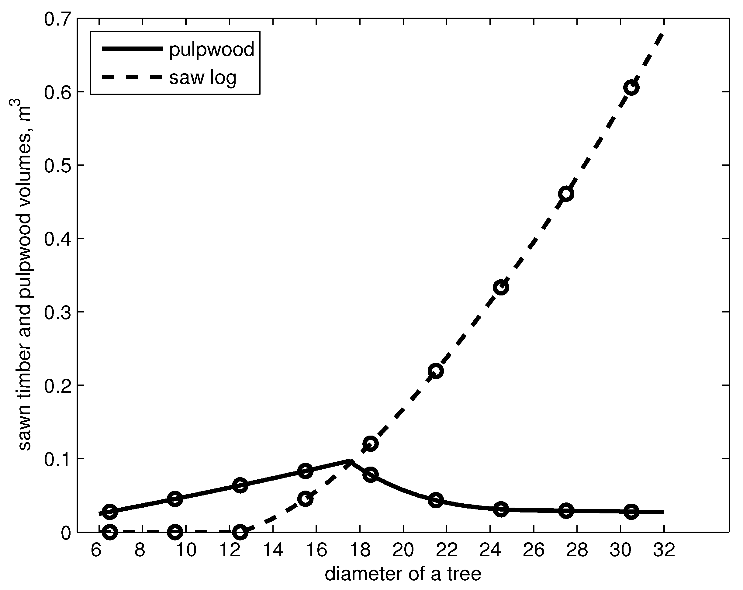
The pulpwood and sawlog volumes of a Scots pine were tabulated at different diameters at intervals of 5 cm starting from 7.5 cm (cf. [27]). By using table (original values according to pine, = 20 m) and cubic spline with not-a-knot end condition [28], we calculated the pulpwood and sawlog volumes of a tree in diameter classes i, . The sawlog and pulpwood volumes of a tree are shown in Figure 2.
We applied FMINCON solver (Matlab Optimization Toolbox) for solving the optimization problem (6)–(9). Technical details and formal subproblems associated with SQP are presented in Appendix A.
Initial Data for Stand-Level Optimization
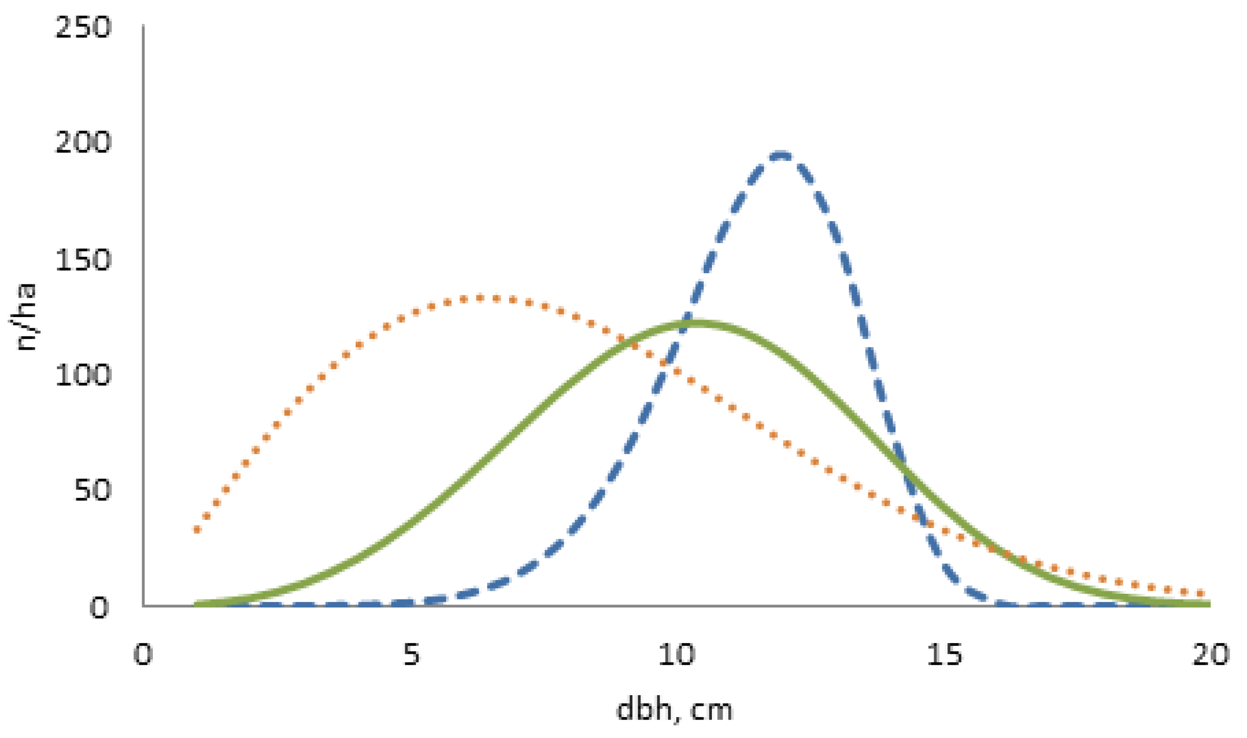
Data for stand-level optimization were sought from a permanent stand plot database for young stands (TINKA). We searched for Scots pine-dominated advanced seedling stands (dominant height of approximately 8 m) from Ostrobothnia. We calculated the rounded average stand characteristics from the artificially regenerated Scots pine stand on a dryish site. Stand characteristics were needed as input variables for creating the individual tree dimensions, stem diameters at breast height (dbh) and tree heights (h). These stand characteristics represented the average stand density having 1000 stems at the age of 25 years. The stand basal area was 9 m , basal area-weighted mean diameter () 12 cm and Lorey’s height () 7.6 m. We created variation in the number of stems while fixing the other stand characteristics in order to develop the options for one more sparse stand and also for one higher stand density (Table 1). The two-parameter Weibull distribution was solved from the stand characteristics using parameter recovery [29]. The samples of 20 randomly selected diameters were generated for each option. We sampled trees from the cumulative probability distribution by randomizing the percentile (P) from the uniform 0–1 distribution. The cumulative Weibull distribution function is of form and tree diameter is solved as where b and c are the scale and shape parameter of the Weibull distribution [30]. From the solved parameters (see Table 1), we noticed that the average density resulted in almost normal distribution () while the highest density (1400 ) with parameter c of 2.01 is strongly skewed to the right and finally the sparse stand (850 ) resulted in a peaked distribution with parameter c of 7.53 (Figure 3).
The parameters and of the Näslund’s height curve [31] were predicted from stand basal area, basal area-weighted mean dbh and Lorey’s height together with the effective temperature sum (993 °C d) using models by [32]. Models also included prediction for the standard deviation of the residual error as a variance function (see [32]). Random deviation was added to the predicted tree height in order to result in realistic variation in stem dimensions.
3. Results
In our calculations, we used the following values for model parameters: interest rate , price of pulpwood and sawlog , and minimum thinning removal .
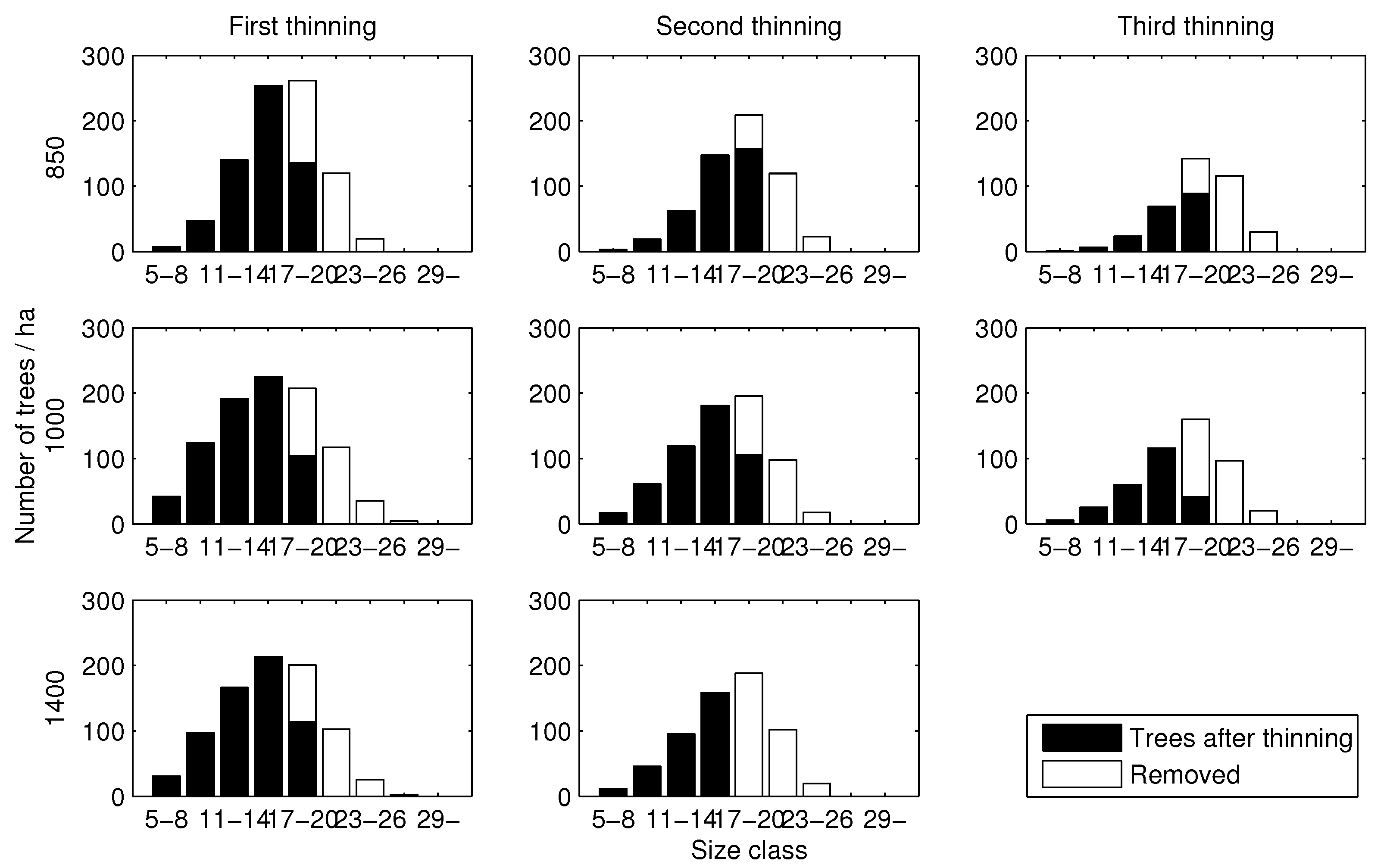
The results show that two or three intermediate thinnings took place during rotation (Table 2). Further, it seems that the thinning pattern (with respect to harvested and remaining trees in different size classes) was more or less similar, regardless of the initial stand density: large trees were always removed (Figure 4). With regard to the thinning intensity of the first thinning, app. 43–45% of basal area was removed. In the second thinning, from 45% (normal stand) up to 68% (dense stand) of basal area was removed. In the third thinning (sparse and normal stands), the removal percentage (expressed as relative to basal area) was on average 64%. The removal percentages fall into the original range of thinning intensities in the modelling data. The maximized revenues fluctuated between 3713 and 4198 € , indicating that initial stand density has an effect on the maximum net present value. On the other hand, with regard to MAI, initial stand density has only a minor role (Table 2).
We tested the sensitivity of the results with respect to two critical aspects. First, the effect of discount rate on optimum stand management was analysed by changing the original 3% into 4% and 5%. Then, we loosened the penalty term (Equation (9)) so that the minimum thinning removal would be 30 , which can be considered to be the “decisive limit” for contractors to execute a thinning in Finland (e.g., [33]). For simplicity, we conducted both sensitivity analyses only for the normal stand density option (number of stems is 1000 ). The results of the sensitivity analysis are shown in Table 3. In the sensitivity analyses, the thinning removals ranged from 31% (third thinning related to 3% discounting and 30 minimum removal criterion) up to 66% (sixth thinning related to 3% discounting and 30 minimum removal criterion), expressed as a percentage of basal area.
Optimal rotation shortened with increasing discount rate—for instance, with 5% discounting, the optimal rotation was 65 years whereas with 3% discounting it was as long as 90 years (Table 2 and Table 3). Another interesting result with discount rates was that with 4% and 5% discounting, the first thinning occurred earlier than with 3%, and the number of intermediate thinnings dropped to two with 4% and 5% discounting (Table 3). The differences in MAI between 3%, 4% and 5% discounting were, however, minor. Relaxing the minimum thinning removal criterion to 30 resulted in a slightly higher maximum net present value as well as more intermediate thinnings to be conducted—compared to the baseline optimal solution (Table 3). Thus, from the forest owner’s point of view, milder thinnings (with respect to thinning removals) are favourable: applying more frequent thinnings with relatively small thinning removals increases the maximum net present value (Table 3).
4. Discussion
When dealing with modelling, one should bear in mind that it is the end users, not the modelers themselves, who finally determine the value of a model (e.g., [1]). Thus, from the end users’ point of view, simplicity and accuracy (in prediction) are the key words to emphasize. From the computational and analytical viewpoint, matrix models are actually simpler by structure than empirical–statistical individual tree models [1], and they essentially require handling of less information [8]. With respect to accuracy, matrix models have been shown to predict tree growth accurately—both in the short term [34] and long term [18,22]. This paper introduces a new time-dependent transition matrix model for predicting pine growth in northern Finland, in which the time-dependency originates from modelling the basal area evolving in time. To our knowledge, such a model presents a novel approach in the literature of matrix population models (cf. [1]). Prior to concluding, we need to compare our results to existing literature on similar growth conditions and tree species in order to discover whether our model is applicable for end users (who are responsible for actual decision-making).
For stand-level optimization, there are various different algorithms to choose from [35,36], e.g., the derivative-free direct search method such as the Hooke and Jeeves method, differential evolution, particle swarm optimization [37], hybrid optimization strategies which combine separate algorithms (e.g., [16]) or depth-first search algorithms which apply a search tree consisting of a backtracking mechanism [37]. In this study, we applied a new algorithm which has recently been introduced to forest applications: sequential quadratic programming (SQP) [38]. Tentatively, the SQP (as representative of gradient-type methods) has been proven to be robust and much more efficient than the derivative-free methods [38].
With respect to financial performance, our results are in line with existing literature on the same tree species (pine) and growth conditions in Finland (e.g., [36,39,40])—given the fact that we assessed the maximum net present value (NPV) for the ongoing rotation, whereas the existing literature focuses on assessing the maximum bare land value (BLV). However, these two measures (MaxNPV and MaxBLV) can be technically commensurated for comparison (e.g., [41]). Optimal number of thinnings varied in this study, depending on the penalty term (Equation (9)) and particularly on the discount rate. This result is coherent with earlier studies [39,40]) suggesting, e.g., that higher interest rates decrease the optimal number of thinnings. Mean annual increments (MAIs) associated with the optimal stand management were here slightly lower than presented in existing literature [40,42], varying from app. 2.52–3.0 to 3.6 . The reasons for this minor discrepancy in volume output are easy to depict: first, the exact locations (in terms of temperature sum and micro-climatic conditions) of stands are slightly different between this study and the others [40,42]). The other reason is related to study frameworks, more precisely to growth models which are, of course, different, and thus result in slightly different outcomes. However, one can argue that the MAIs underlying optimal management produced by alternative growth models can be considered to be similar. In addition, different optimization algorithms were applied in the studies, which also has an effect on outcomes (see, e.g., [35]).
Finally, the underlying rationale (and motive) for constructing a time-dependent matrix model is to later on be able to incorporate genetic gains into that particular model. The idea of incorporating genetic gains into the time-dependent matrix model stems from the fact that genetic gain in growth evolves with time (e.g., [43]), indicating that genetic gain once assessed at juvenile stage could change towards maturity [44,45]. Thus, in the near future, we need growth models which take into account this phenomenon. Further, we could also include variation in stem quality (due to tree breeding; see [46,47]), and further incorporate it into the time-dependent matrix model. For instance, this can technically be done with a subdivision of the categories, i.e., size classes (see [4,48]). Having incorporated the effect of time-evolving genetic gain and variation in stem quality into the time-dependent matrix model, this creates a new set of analysis tools for assessments. In this new assessment framework, it would finally be possible in forestry to value the relevant traits (such as enhanced growth and stem quality) in monetary terms, and to construct genuine trade-offs between breedable traits. This further enables efficient deployment of improved material in different climatic conditions (see [49]).
Acknowledgments
We want to acknowledge the Jenny and Antti Wihuri foundation for financial support.
Author Contributions
Jouni Siipilehto provided the data for optimizations; Johanna Pyy developed the matrix model and optimization problem and conducted the optimizations under supervision of Erkki Laitinen; Anssi Ahtikoski analyzed the results; all authors contributed to the writing of the manuscript.
Conflicts of Interest
The authors declare no conflict of interest. The founding sponsors had no role in the design of the study; in the collection, analyses, or interpretation of data; in the writing of the manuscript, and in the decision to publish the results.
Appendix A
To solve the optimization problem (6)–(9), we used FMINCON© solver of the Matlab Optimization Toolbox. The solver uses the SQP algorithm [50]. In that vector, is first solved from the quadratical subproblem
where denotes positive definite approximation to the Hessian of the Lagrangian function for the optimization problem at iteration point and is the Jacobian of object function f at point . The functions and are the equality constraint (4) and inequality constraint (8), respectively. The new iteration step is given by , where step length is chosen so that the new iterate will not violate the constraints.
References
- Liang, J.; Picard, N. Matrix model of forest dynamics: An overview and outlook. For. Sci. 2013, 59, 359–378. [Google Scholar] [CrossRef]
- Picard, N.; Mortier, F.; Chagneau, P. Influence of estimators of the vital rates in the stock recovery rate when using matrix models for tropical rainforests. Ecol. Model. 2008, 214, 349–360. [Google Scholar] [CrossRef]
- Hauser, C.E.; Cooch, E.G.; Lebreton, J.D. Control of structured populations by harvest. Ecol. Model. 2006, 196, 462–470. [Google Scholar] [CrossRef]
- Caswell, H. Matrix Population Models: Construction, Analysis and Interpretation, 2nd ed.; Sinauer Associates Inc. Publishers: Sunderland, MA, USA, 2001. [Google Scholar]
- Newman, K.B.; Buckland, S.T.; Morgan, B.J.T.; King, R.; Borchers, D.L.; Cole, D.J.; Besbeas, P.; Gimenez, O.; Thomas, L. Modelling Population Dynamics. Model Formulation, Fitting and Assessment Using State-Space Methods; Methods in Statistical Ecology; Springer: New York, NY, USA, 2014. [Google Scholar]
- Vanclay, J.K. Modeling Forest Growth and Yield: Applications to Mixed Tropical Forests; CAB International: Wallingford, UK, 1994. [Google Scholar]
- Porte, A.; Bartelink, H.H. Modelling mixed forest growth: A review of models for forest management. Ecol. Model. 2002, 150, 141–188. [Google Scholar] [CrossRef]
- Grimm, V. Ten years of individual-based modelling in ecology: What have we learned and what could we learn in the future? Ecol. Model. 1999, 115, 129–148. [Google Scholar] [CrossRef]
- Zuidema, P.A.; Jongejans, E.; Chien, P.D.; During, H.J.; Schieving, F. Integral projection models for trees: A new parametrization method and a validation of model output. J. Ecol. 2010, 98, 345–355. [Google Scholar] [CrossRef]
- Lee, C.-C.; Okuyama, T. Individual variation in stage duration in matrix population models: Problems and solutions. Biol. Control 2017, 110, 117–123. [Google Scholar] [CrossRef]
- Picard, N.; Liang, J. Matrix models for size-structured populations: Unrealistic fast growth or simply diffusion. PLoS ONE 2014, 9, e98254. [Google Scholar] [CrossRef] [PubMed]
- Salguero-Gomez, R.; Plotkin, J.B. Matrix dimensions bias demographic inferences: Implications for comparative plant demography. Am. Nat. 2010, 176, 710–722. [Google Scholar] [CrossRef] [PubMed]
- Picard, N.; Bar-Hen, A.; Guedon, Y. Modelling diameter class distribution with a second-order matrix model. For. Ecol. Manag. 2003, 180, 389–400. [Google Scholar] [CrossRef]
- Zhou, M.; Buongiorno, J. Nonlinearity and noise interaction in a model of forest growth. Ecol. Model. 2004, 180, 291–304. [Google Scholar] [CrossRef]
- Roth, G.; Caswell, H. Hyperstate matrix models: Extending demographic state spaces to higher dimensions. Methods Ecol. Evol. 2016, 7, 1438–1450. [Google Scholar] [CrossRef]
- Niinimäki, S.; Tahvonen, O.; Mäkelä, A. Applying a process-based model in Norway spruce management. For. Ecol. Manag. 2012, 265, 102–115. [Google Scholar] [CrossRef]
- Sable, S.E.; Rose, K.A. A comparison of individual-based and matrix models for simulating yellow perch population-dynamics in Oneida Lake, New York, USA. Ecol. Model. 2008, 215, 64–75. [Google Scholar] [CrossRef]
- Bollandsås, O.M.; Buongiorno, J.; Gobakken, T. Predicting the growth of stands of trees of mixed species and size: A matrix model for Norway. Scand. J. For. Res. 2008, 23, 167–178. [Google Scholar] [CrossRef]
- Tahvonen, O. Optimal choice between even- and uneven-aged forestry. Nat. Resour. Model. 2009, 22, 289–321. [Google Scholar] [CrossRef]
- Tahvonen, O.; Pukkala, T.; Laiho, O.; Lähde, E.; Niinimäki, S. Optimal management of uneven-aged Norway spruce stands. For. Ecol. Manag. 2010, 260, 106–115. [Google Scholar] [CrossRef]
- Lin, C.R.; Buongiorno, J.; Vasievich, M. A multi-species, density-dependent matrix growth model to predict tree diversity and income in northern hardwood stands. Ecol. Model. 1996, 91, 193–211. [Google Scholar] [CrossRef]
- Liang, J. Dynamics and management of Alaska boreal forest: An all-aged multi-species matrix growth model. For. Ecol. Manag. 2010, 260, 491–501. [Google Scholar] [CrossRef]
- Mäkinen, H.; Isomäki, A. Thinning intensity and growth of Scots pine stands in Finland. For. Ecol. Manag. 2004, 201, 311–325. [Google Scholar] [CrossRef]
- Tonteri, T.; Hotanen, J.P.; Kuusipalo, J. The Finnish forest site type approach: Ordination and classification studies of mesic forest sites in southern Finland. Vegetatio 1990, 87, 85–98. [Google Scholar] [CrossRef]
- Anonymous Statistical Yearbook of Forestry 2014, Table 1.5 at Page 51. Available online: http://www.metla.fi/metinfo/tilasto/julkaisut/vsk/2014/ (accessed on 9 May 2017).
- Venäläinen, A.; Tuomenvirta, H.; Pirinen, P.; Drebs, A. A Basic Finnish Climate Data Set 1961–2000—Description and Illustrations; Reports No. 2005:5; Finnish Meteorological Institute: Helsinki, Finland, 2005; pp. 1–27.
- Rämö, J.; Tahvonen, O. Economics of harvesting uneven-aged forest stands in Fennoscandia. Scand. J. For. Res. 2014, 29, 777–792. [Google Scholar] [CrossRef]
- Behforooz, H.G. A Comparison of the E(3) and Not-A-Knot Cubic Splines. Appl. Math. Comput. 1995, 72, 219–223. [Google Scholar]
- Siipilehto, J.; Mehtätalo, L. Parameter recovery vs. parameter prediction for the Weibull distribution validated for Scots pine stands in Finland. Silva Fenn. 2013, 47, 1–22. [Google Scholar] [CrossRef]
- Bailey, R.L.; Dell, T.R. Quantifying diameter distributions with the Weibull function. For. Sci. 1973, 19, 97–104. [Google Scholar]
- Näslund, M. Skogsförsöksanstaltens gallringsförsök i tallskog. Meddelanden från Statens Skogsförsöksanstalt 1936, 29, 169. [Google Scholar]
- Siipilehto, J.; Kangas, A. Näslundin pituuskäyrä ja siihen perustuvia malleja läpimitta-pituus riippuvuudesta suomalaisissa talousmetsissä. Metsätieteen Aikakauskirja 2015, 4, 215–316. [Google Scholar]
- Kojola, S. Kohti Hyvää Suometsien Hoitoa? Harvennusten Ja Kunnostusojitusten Vaikutus Ojitusaluemä NniköIden Puuntuotokseen Ja MetsäNkasvatuksen Taloustulokseen. Dissertationes Forestales 83. Ph.D. Thesis, University of Helsinki, Helsinki, Finland, 2009. (In Finnish with English summary). [Google Scholar]
- Van Mantegem, P.J.; Stephenson, N.L. The accuracy on matrix population model predictions for coniferous trees in the Sierra Nevada, California. J. Ecol. 2005, 93, 737–747. [Google Scholar] [CrossRef]
- Pukkala, T. Population-based methods in the optimization of stand management. Silva Fenn. 2009, 43, 261–274. [Google Scholar] [CrossRef]
- Cao, T. Silvicultural Decisions Based on Simulation-Optimization Systems. Dissertationes Forestales 103. Ph.D. Thesis, University of Helsinki, Helsinki, Finland, 2010. Available online: http://www.metla.fi/dissertationes/df103.htm (accessed on 9 May 2017).
- Arias-Rodil, M.; Pukkala, T.; Gonzalez-Conzalez, J.M; Barrio-Anta, M.; Dieguez-Aranda, U. Use of depth-first search and direct search methods to optimize even-aged stand management: A case study involving maritime pine in Asturias (northwest Spain). Can. J. For. Res. 2015, 45, 1269–1279. [Google Scholar] [CrossRef]
- Arias-Rodil, M.; Dieguez-Aranda, U.; Vazquez-Mendez, M.E. A differentiable optimization model for the management of single-species, even-aged stands. Can. J. For. Res. 2016, 47, 506–514. [Google Scholar] [CrossRef]
- Hyytiäinen, K.; Tahvonen, O.; Valsta, L. Optimum juvenile density, harvesting and stand structure in even-aged Scots pine stands. For. Sci. 2005, 51, 120–133. [Google Scholar]
- Tahvonen, O.; Pihlainen, S.; Niinimäki, S. On the economics of optimal timber production in boreal Scots pine stands. Can. J. For. Res. 2013, 43, 719–730. [Google Scholar] [CrossRef]
- Johansson, P.-O.; Löfgren, K.-G. The Economics of Forestry and Natural Resources; Basil Blackwell: Oxford, UK; New York, NY, USA, 1985. [Google Scholar]
- Pukkala, T.; Lähde, E.; Laiho, O. Optimizing the structure and management of uneven-sized stands of Finland. Forestry 2010, 83, 129–142. [Google Scholar] [CrossRef]
- Carson, S.; Garcia, O.; Hayes, J.D. Realized gain and prediction of yield with genetically improved Pinus radiata in New Zealand. For. Sci. 1999, 45, 186–200. [Google Scholar]
- Vergara, R.; White, T.L.; Shiver, B.D.; Rockwood, D.L. Estimated realized gains for first-generation slash pine (Pinus elliottii var. elliottii) tree improvement in the southeastern United States. Can. J. For. Res. 2004, 34, 2587–2600. [Google Scholar] [CrossRef]
- Kimberley, M.O.; Moore, J.R.; Dungey, H.S. Quantification of realised genetic gain in radiata pine and its incorporation into growth and yield modeling systems. Can. J. For. Res. 2015, 45, 1676–1687. [Google Scholar] [CrossRef]
- Cumbie, W.P.; Isik, F.; McKeand, S.E. Genetic improvement of sawtimber potential in Loblolly pine. For. Sci. 2012, 58, 168–177. [Google Scholar] [CrossRef]
- Kennedy, A.G.; Cameron, A.D.; Lee, S.J. Genetic relationships between wood quality traits and diameter growth of juvenile core wood in Sitka spruce. Can. J. For. Res. 2013, 43, 1–6. [Google Scholar] [CrossRef]
- Pfister, C.A; Wang, M. Beyond size: Matrix projection models for populations where size is an incomplete descriptor. Ecology 2005, 86, 2673–2683. [Google Scholar] [CrossRef]
- Jansson, G.; Hansen, J.K.; Haapanen, M.; Kvaalen, H.; Steffenrem, A. The genetic and economic gains from forest tree breeding programmes in Scandinavia and Finland. Scand. J. For. Res. 2017, 32, 273–286. [Google Scholar] [CrossRef]
- Nocedal, J.; Wright, S J. Numerical Optimization; Springer: New York, NY, USA, 1999. [Google Scholar]
Figure 1.
Locations of experiments.
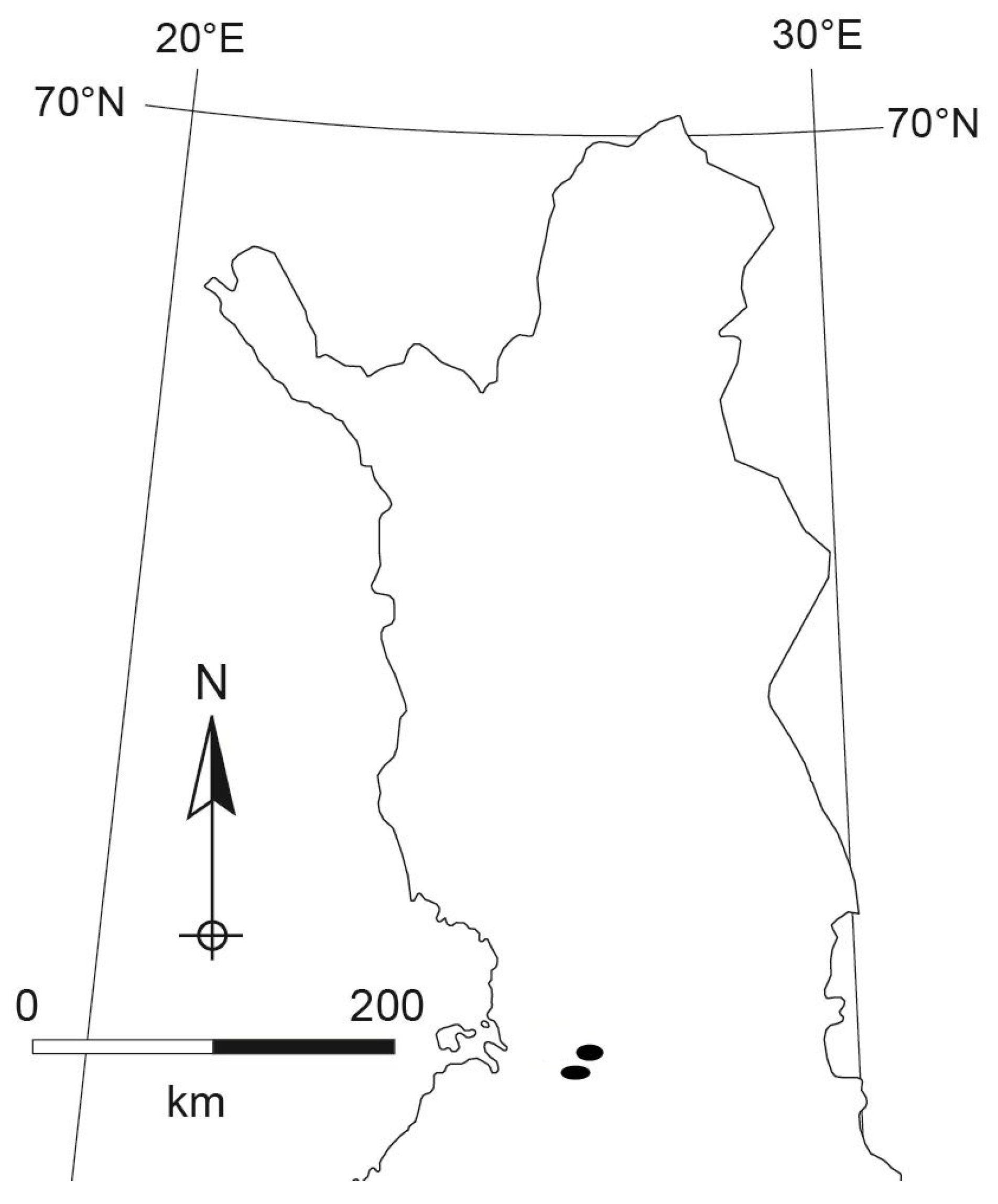
Figure 2.
Pulpwood and sawlog volumes of a tree as a function of diameter at breast height, cm.

Figure 3.
The shapes of the Weibull dbh distributions for the average stand (solid line) which followed approximately normal distribution () and for sparse (broken line) and dense stand (dotted line).
Figure 3.
The shapes of the Weibull dbh distributions for the average stand (solid line) which followed approximately normal distribution () and for sparse (broken line) and dense stand (dotted line).

Figure 4.
Diameter distributions associated with optimal thinnings. Numbers (e.g., 5–8, 11–14) represent diameter in centimetres.
Figure 4.
Diameter distributions associated with optimal thinnings. Numbers (e.g., 5–8, 11–14) represent diameter in centimetres.

Table 1.
The standard stand characteristics and the recovered Weibull parameters b and c.
| Stand Age, Years | Basal Area, m ha | Number of Stems ha | Weighted Mean dbh, cm | Lorey’s Height, m | Dominant Height, m | Scale Parameter b | Shape Parameter c |
|---|---|---|---|---|---|---|---|
| 25 | 9 | 850 | 12 | 7.6 | 8.5 | 12.216 | 7.535 |
| 25 | 9 | 1000 | 12 | 7.6 | 8.5 | 11.352 | 3.612 |
| 25 | 9 | 1400 | 12 | 7.6 | 8.5 | 9.057 | 2.011 |
Table 2.
Optimal stand-level managements generated by the matrix model. Discount rate 3%.
| Thinning | Age of the Stand (a) | Volume of Removed Trees (m ha) | Proportion of Saw log (%) | NPV (€ ha) | MAI (m ha year) |
|---|---|---|---|---|---|
| Sparse (Number of stems 850) | |||||
| First thinning | 45 | 63.7 | 75 | ||
| Second thinning | 55 | 50.0 | 80 | ||
| Third thinning | 65 | 52.3 | 81 | ||
| Final thinning | 95 | 73.7 | 90 | ||
| Total | 239.6 | 82 | 4042 | 2.52 | |
| Normal (Number of stems 1000) | |||||
| First thinning | 45 | 66.3 | 78 | ||
| Second thinning | 55 | 50.0 | 76 | ||
| Third thinning | 65 | 56.3 | 75 | ||
| Final thinning | 90 | 73.7 | 84 | ||
| Total | 246.3 | 79 | 4198 | 2.74 | |
| Dense (Number of stems 1400) | |||||
| First thinning | 45 | 54.9 | 78 | ||
| Second thinning | 55 | 71.4 | 72 | ||
| Final thinning | 85 | 95.1 | 85 | ||
| Total | 221.4 | 79 | 3713 | 2.60 | |
Table 3.
Optimal stand-level managements generated by the matrix model with different interest rates and minimum thinning removals. “Baseline optimal solution” indicates stand management with 3% interest rate and normal initial density (number of stems 1000 ha).
Table 3.
Optimal stand-level managements generated by the matrix model with different interest rates and minimum thinning removals. “Baseline optimal solution” indicates stand management with 3% interest rate and normal initial density (number of stems 1000 ha).
| Thinning | Age of the Stand (a) | Volume of Removed Trees (m ha) | Proportion of Saw log (%) | NPV (€ ha) | MAI (m ha year) |
|---|---|---|---|---|---|
| Interest rate 4% and minimum thinning removal 50 m ha | |||||
| First thinning | 40 | 61.4 | 70 | ||
| Second thinning | 50 | 50.2 | 67 | ||
| Final thinning | 75 | 109.3 | 78 | ||
| Total | 220.9 | 73 | 3168 | 2.95 | |
| Interest rate 5% and minimum thinning removal 50 m ha | |||||
| First thinning | 35 | 50.2 | 58 | ||
| Second thinning | 45 | 50.0 | 57 | ||
| Final thinning | 65 | 77.0 | 68 | ||
| Total | 177.2 | 62 | 2513 | 2.73 | |
| Interest rate 3% and minimum thinning removal 30 m ha | |||||
| First thinning | 35 | 36.9 | 66 | ||
| Second thinning | 45 | 38.6 | 68 | ||
| Third thinning | 55 | 30.0 | 80 | ||
| Fourth thinning | 65 | 36.5 | 86 | ||
| Fifth thinning | 75 | 30.2 | 88 | ||
| Sixth thinning | 85 | 43.1 | 88 | ||
| Final thinning | 105 | 41.2 | 88 | ||
| Total | 256.6 | 81 | 4355 | 2.44 | |
| Baseline optimal solution | |||||
| First thinning | 45 | 66.3 | 78 | ||
| Second thinning | 55 | 50.0 | 76 | ||
| Third thinning | 65 | 56.3 | 75 | ||
| Final thinning | 90 | 73.7 | 84 | ||
| Total | 246.3 | 79 | 4198 | 2.74 | |
© 2017 by the authors. Licensee MDPI, Basel, Switzerland. This article is an open access article distributed under the terms and conditions of the Creative Commons Attribution (CC BY) license (http://creativecommons.org/licenses/by/4.0/).
Share and Cite
MDPI and ACS Style
Pyy, J.; Ahtikoski, A.; Laitinen, E.; Siipilehto, J. Introducing a Non-Stationary Matrix Model for Stand-Level Optimization, an Even-Aged Pine (Pinus Sylvestris L.) Stand in Finland. Forests 2017, 8, 163. https://doi.org/10.3390/f8050163
AMA Style
Pyy J, Ahtikoski A, Laitinen E, Siipilehto J. Introducing a Non-Stationary Matrix Model for Stand-Level Optimization, an Even-Aged Pine (Pinus Sylvestris L.) Stand in Finland. Forests. 2017; 8(5):163. https://doi.org/10.3390/f8050163
Chicago/Turabian StylePyy, Johanna, Anssi Ahtikoski, Erkki Laitinen, and Jouni Siipilehto. 2017. "Introducing a Non-Stationary Matrix Model for Stand-Level Optimization, an Even-Aged Pine (Pinus Sylvestris L.) Stand in Finland" Forests 8, no. 5: 163. https://doi.org/10.3390/f8050163
Note that from the first issue of 2016, this journal uses article numbers instead of page numbers. See further details here.