
Drones as a Tool for Monoculture Plantation Assessment in the Steepland Tropics

1
ForestGEO, Smithsonian Tropical Research Institute, Balboa, Ancon, 0843-03092 Panama City, Panama
2
Yale School of Forestry & Environmental Studies, New Haven, CT 06511, USA
3
Smithsonian Tropical Research Institute, Balboa, Ancon, 0843-03092 Panama City, Panama
4
Fearless Labs, 8 Market Place, Baltimore, MD 21202, USA
*
Author to whom correspondence should be addressed.
Forests 2017, 8(5), 168; https://doi.org/10.3390/f8050168
Submission received: 31 March 2017
/
Revised: 2 May 2017
/
Accepted: 6 May 2017
/
Published: 12 May 2017
(This article belongs to the Special Issue Optimizing Forest Inventories with Remote Sensing Techniques)
Abstract
:Smallholder tree plantations are expanding in the steepland tropics due to demand for timber and interest in ecosystem services, such as carbon storage. Financial mechanisms are developing to compensate vegetation carbon stores. However, measuring biomass—necessary for accessing carbon funds—at small scales is costly and time-intensive. Therefore, we test whether low-cost drones can accurately estimate height and biomass in monoculture plantations in the tropics. We used Ecosynth, a drone-based structure from motion technique, to build 3D vegetation models from drone photographs. These data were filtered to create a digital terrain model (DTM) and digital surface model (DSM). Two different canopy height models (CHMs) from the Ecosynth DSM were obtained by subtracting terrain elevations from the Ecosynth DTM and a LIDAR DTM. We compared height and biomass derived from these CHMs to field data. Both CHMs accurately predicted the height of all species combined; however, the CHM from the LiDAR DTM predicted heights and biomass on a per-species basis more accurately. Height and biomass estimates were strong for evergreen single-stemmed trees, and unreliable for small leaf-off species during the dry season. This study demonstrates that drones can estimate plantation biomass for select species when used with an accurate DTM.
1. Introduction
Tropical forest plantations play a major role in global timber markets. In 2012, 231 million m3 (41% of the global total) of industrial roundwood from plantations was produced in tropical countries [1]. In addition to timber, national and international institutions are looking to plantations for ecosystem services such as carbon sequestration, water filtration, and soil conservation [2,3,4,5]. Countries and multilateral organizations such as the United Nations are implementing vegetation carbon accounting programs to integrate carbon stores, including those in plantations, into national and global budgets. These mechanisms are increasingly making funding available to landowners and organizations that can track changes in biomass and quantify carbon stored.
Performing accurate inventories of plantations is critical for any land manager [6]. Diameter at breast height is often measured in the field to estimate height, which can then be used to inform harvest schedules and derive biomass [7]. However, assessing height directly is often cost and time-prohibitive [8].
One alternative to measuring height by hand is offered by remote sensing techniques [9]. Light Detection and Ranging (LiDAR), which records 3D structure based on emitted laser pulses, is often employed for characterizing 3D vegetation structure [10]. While LiDAR can accurately measure forest, plantation, and individual tree structure in 3D [11,12,13,14], it is prohibitively-expensive for smallholders in tropical and developing nations [8]. A typical commercial aerial LiDAR acquisition costs at least US $20,000 per flight [15], significantly more than low-income smallholders can afford.
However, new developments with unmanned aerial vehicles (drones) have significantly lowered the cost and time needed to conduct inventories [16,17,18]. Because of this, drones offer the possibility of empowering landowners or small organizations to conduct forest inventories more frequently. Nowadays, one can buy a high-quality drone and equip it with an RGB digital camera, thereby creating a homemade remote sensing tool [19,20]. Photos taken from these cameras can be processed with open-source software (e.g., Ecosynth) to construct a 3D model using structure from motion algorithms [21,22]. These algorithms identify features (e.g., trees, buildings) on overlapping photos taken from different angles and reconstruct the features’ 3D structure [23,24]. The resulting data is a collection of RGB points that represent the 3D surface of the objects imaged by the drone. This method has been used to produce LiDAR-like results in measuring canopy heights, structure, roughness, and biomass [18,21,22,25].
While drones have been used in connection with estimation of height and biomass in mixed plantations and secondary forest [18], they have never been tested for their ability to support estimation of height, aboveground biomass (AGB), and total biomass (TB) on a per-species basis in monoculture plantations in the steepland tropics. Characterized by slopes that average more than 12% in grade, the steepland tropics provide critical land for smallholders and watersheds for communities and cities [26]. Because the slopes are too treacherous for industrial cultivation, forestry and agriculture are often practiced by smallholders and are thus an ideal place to test this approach [26,27,28,29].
Additionally, past forestry-relevant drone studies have largely focused on the use of drones in monitoring forest variables and temperate plantation management [17,30,31]. Few of these studies have been performed for tropical timber plantations and none have been performed on the species that we studied. As interest in operationalizing drones for forest inventories proliferates, it is critical to determine the appropriate conditions and purposes for using these tools [32].
In this study, we compare estimates of canopy height and biomass (aboveground and total) of five different species derived from drone-based models and LiDAR-based models. The study was performed in the steeplands that surround the Panama Canal. We applied this method to 56–1754 m2 plantations of five different species, and evaluated its performance by comparing height with field-based measurements and biomass with estimates derived from locally-generated allometric equations.
2. Materials and Methods
2.1. Study Site
This study was performed at the site of the Smithsonian Tropical Research Institute’s Agua Salud Project in the Panama Canal Watershed (9°13′ N, 79°47′ W). The site receives 2700 mm of annual rainfall, experiences a dry season from mid-December through early May [33] and is characterized by short, steep, and highly variable slopes (range of 0–75°, mean of 24°) that range from 52 to 343 m above sea level in elevation. Agua Salud is a mosaic of pastures, successional forests, and plantations (both native and exotic) and is surrounded by a diverse landscape of agriculture, human settlements, and forest [34]. The Agua Salud native species plantations consist of 21 treatments of different combinations of monocultures and mixtures and totals 267 plots, 56 of which are monocultures of native species [35].
This study was carried out in the 56–1754 m2 (45 m × 39 m) monoculture native species plantations (termed ‘plots’) located in two different blocks (termed ‘Block 1’ and ‘Block 2’) within the Agua Salud Project area (see Figure 1). Thirty plots are located in Block 1 and 26 plots are in Block 2, all of which were established in 2008. Five different species were randomly assigned to the plots and stratified across slope classes—Terminalia amazonia, Dalbergia retusa, Pachira quinata, Tabebuia rosea, and Anachardium excelsum. Each plot contained a 27 m × 23.4 m ‘core zone’ of 81 trees (nine rows of nine trees each), and was surrounded by a buffer zone of three rows of trees on every side—resulting in a total of 225 trees in each plot. All plots were 7 years old at the time of measurement.
2.2. Data Collection and Analysis
2.2.1. Field Measurements
Canopy Height
Heights were measured with a 15-meter extendable pole between June and July 2015 for all trees in each core zone. Heights were measured at the tallest stem. If no tree was present, the record was marked as null and the entry was omitted from further analysis. Average field height per core zone was then calculated, termed ‘field height,’ which was assumed to represent the average height of the entire plot.
Biomass
Aboveground biomass (AGB) and total biomass (TB) were calculated for each core zone using species-specific allometric equations that were derived in a separate study [36]. In their study, Sinacore et al. measured and destructively-harvested 41 trees from six species, five of which are included in this study. They further excavated, dried, and weighed all roots down to 2 mm thus providing accurate measures of belowground biomass.
The best species-specific allometric equations from the Sinacore et al. paper, used in this study, take basal diameter as input parameters [33]. Basal diameters were measured at the same time as tree heights and were recorded for each stem in the multi-stemmed trees. Out of the 3955 trees that were present, 351 were multi-stemmed (59% of which were D. retusa). From the 351 multi-stemmed trees, 271 had two stems, 62 had three stems, 15 had four stems, two had five stems, and one had six stems. Both AGB and TB were calculated for individual stems using basal diameter values. Biomass was then summed for all the trees in a core zone and divided by the area to get the final dimensions (Mg/Ha). Since height has been found to predict biomass [18,37], field-estimated AGB and TB were compared to remotely-sensed height measurements (see below) to determine how well height measurements from drones could be used to model AGB and TB estimates of these species.
2.2.2. Remote Sensing Measurements
LiDAR Collection
LiDAR data was collected for the study areas in August 2009 by Blom (a surveying company) using an Optech sensor (Optech Incorporated, ALTM 3100, Toronto, Canada) on board a fixed wing manned aircraft traveling at 457.2 m above the ground at a flight speed of 66.9 m·s−1 (scanning frequency of 48 Hz and pulse repetition rate of 70 kHz). Blom then created a model of the terrain, a DTM, from this data using TerraScan 9.0 (TerraSolid, Helsinki, Finland), with spatial resolution of 1 × 1 m. LiDAR horizontal and vertical accuracy was evaluated at 36 control points within the flight area, resulting in a horizontal root mean square error (RMSE) of 7.6 cm, and a vertical RMSE of 6.9 cm. Due to the age of the LiDAR data relative to the current study (2009 vs. 2015), no surface measurements of canopy height from the LiDAR were used. Instead, it is expected that there would be little change in topography over this time, making the 2009 LiDAR DTM a valid dataset for the current work. This DTM was used in all LiDAR analysis in this study, referred to as the LiDAR DTM, or the LiDAR terrain model.
Image Collection
Imagery was collected using a multirotor drone following the methods and equipment specifications of Dandois and Ellis [21], from 16 April 2015 to 19 April 2015. Digital images were taken with a Canon ELPH 520 (Canon Inc., Tokyo, Japan) HS point and shoot digital camera, which shot continuously at two frames per second (f·s−1) throughout the flights. Seven flights were required to capture both Block 1 (five flights) and Block 2 (two flights). Drone flight altitude was fixed to 400 m above the launch location, which was set at a nominal location and elevation within each flight area. The drone flew autonomously along a predetermined flight path at roughly 7 m·s−1, resulting in an average image resolution of 14 cm GSD. In general, flights were conducted between 09:00 and 14:00 local time to minimize the effects of sun angle and to avoid high winds and rain.
Point Cloud Generation
Several processing steps were required prior to creating point clouds from drone images. GPS and altitude telemetry from the drone were used to provide an initial estimate of the XYZ location of each image. Due to the relatively high frame rate of the camera and high altitude, images were collected with very high forward overlap (≥ 98%), resulting in more image data than is needed so image sequences were subsampled to every 10th frame [25]. Even though image white balance and contrast were fixed before each flight to an 18% gray card in full sun, there were still differences in image quality between flights over the same locations and within flights due to passing clouds and cloud shadows. A histogram matching technique was used to minimize these effects [38]. Briefly, images were converted to the HSV (hue-saturation-value) color space, then for each image, the histogram of the value channel was normalized to that of an exemplar image manually identified to have good contrast and exposure with no cloud shadows.
Normalized images were then transformed back to the RGB color space. Normalized and georeferenced images from each flight were then imported into the photogrammetry, structure from motion software Agisoft Photoscan (version 1.1.6, 64-bit) for each flight area (Block 1 and Block 2) to create 3D point clouds. This software uses computer vision photogrammetric algorithms to recognize similar features in multiple images and to simultaneously solve for their locations as well as the location and orientation of the camera at the time of image capture in 3D space ([21] for further details). After initial processing, a GeoTIFF orthomosaic (14 cm GSD) was exported from Photoscan.
Additional georeferencing was performed in ArcGIS and Photoscan on the drone orthomosaic by extracting XYZ data from the LiDAR DTM for ground control points (e.g., building corners, distinct marks in the roads, small shrubs, etc.). The resulting DTM had a positional RMSE of 1.30 m for Block 1 and 1.89 m for Block 2, relative to the LiDAR DTM error. After this stage, a sparse point cloud was exported for each block for additional analysis. This point cloud, produced from drone imagery, is referred to as the Ecosynth point cloud, based on the name of the methodology used [21,22].
Digital Terrain and Canopy Height Models
Digital terrain models were created from the Ecosynth point clouds by refining the data and then filtering the terrain. The referenced point clouds were clipped to the study area, filtered to remove any noisy points, and converted into a 1 × 1 m grid of median height values. Terrain filtering algorithms were then applied to each point cloud using MCC-LiDAR software to produce the DTMs [39]. This software applies a filter to the point cloud at different scales to estimate whether any given data point is a local low point—thus classified as ‘terrain’. The terrain points were then interpolated into a 1 m gridded raster DTM using natural neighbor interpolation in ArcGIS 10.1 (ESRI, Redlands, CA, USA). Canopy height models (CHM) were created from the Ecosynth DTM and LiDAR DTM by subtracting the underlying DTM value from the elevation of each point in the Ecosynth point cloud. These canopy height models are hereafter referred to as Ecosynth CHM and LiDAR CHM. As noted above (Section 2.2.2), due to the age of the LIDAR data, no canopy heights were obtained from LIDAR canopy surface measurements—the LiDAR CHM refers to the model derived from subtracting the Ecosynth canopy height measurements from the LiDAR DTM.
A Trimble R8 differential GPS unit was used to record the locations of all the corners of the study plots via FastStatic. This was done to enable accurate plot-level spatial analysis of the canopy height models. Coordinates were processed and exported with Trimble Business Center with a median precision of 7 cm horizontal and 10 cm vertical in Block 1 and 12 cm horizontal and 7 cm vertical in Block 2.
2.2.3. Data Analysis
Canopy Height and Biomass
Canopy height metrics—mean, minimum, maximum, median, 25th percentile, 75th percentile, and 95th percentile height—were calculated using points from each CHM with height >0 m on a per-treatment per-plot basis (N = 56, see Supplementary Materials). These metrics were then plotted against all field heights, AGB, and TB from each CHM using both simple linear regression and linear mixed-effect models to determine which metric and model could best predict field-derived values based on Akaike information criterion (AIC). Using mixed-effect models allowed us to test whether treating the species as a random variable improved the model. The same canopy metrics were then linearly regressed against field heights, AGB, and TB for each species separately to find the best metric for species-specific predictions, again using AIC as the means for model selection. The best models were tested for significance by analyzing their p values.
Visual inspection of the imagery and CHMs revealed that the maps of the plots did not capture crowns that extended outside the plot borders. To include these points in the height analysis, the plot borders were manually adjusted to include the overhanging crowns, as determined by visual inspection. Trees that crowded into the plots were similarly excluded (see Figure 2). While this process was made easier by the clear outline of plantation-style crowns, there is a corresponding level of error from manual tracing of tree crowns.
Vertical Canopy Profiles
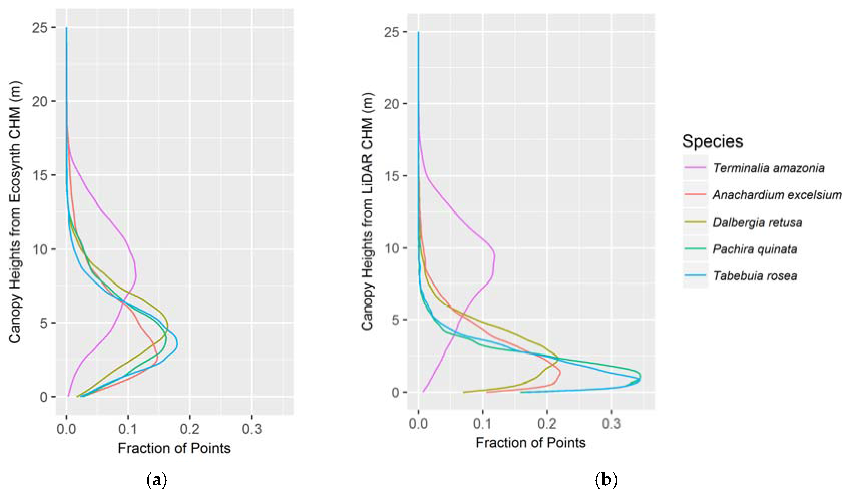
Canopy profiles were made for each CHM on a per-species basis by plotting a vertical histogram of point heights. This was done to visualize and compare each CHM’s ability to characterize the vertical canopy distributions of the studied species.
3. Results
3.1. Canopy Height
When modeling height using all treatments from the Ecosynth CHM, we found that the most parsimonious model (see Figure 3a) is a linear mixed effect model with the median height metric as the independent variable (AIC: 194.5, see Table 1). This model took species as the random effect and assessed the model using random slopes. Median canopy height was also the best predictor of field height with the LiDAR CHM (see Table 1) but with a simple linear model (R2: 0.906, see Figure 3b). The LiDAR CHM produced significantly better models of height compared to the Ecosynth CHM, as seen by the AIC values.
Again, the median canopy height metric was the best predictor of field height on a per-species basis for both canopy height models. When species-specific linear models were created, both LiDAR and Ecosynth CHMs exhibited the same order of predictive ability for species, as judged from the R2 and RMSE values (see Table 2). In order of decreasing predictability, the species are T. amazonia, D. retusa, A. excelsum, T. rosea, and P. quinata. The LiDAR CHM improved the prediction of height for each species compared to Ecosynth CHM (see Table 2).
3.2. Aboveground and Total Biomass
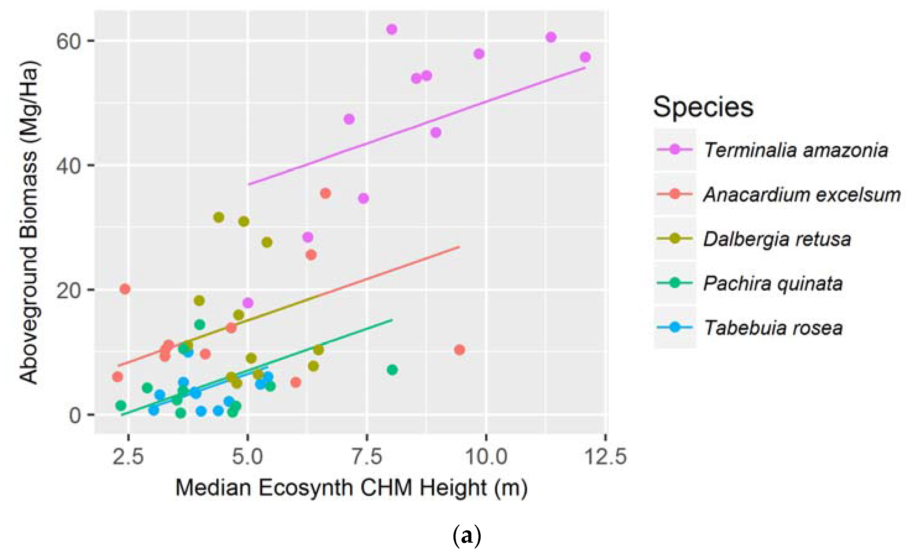
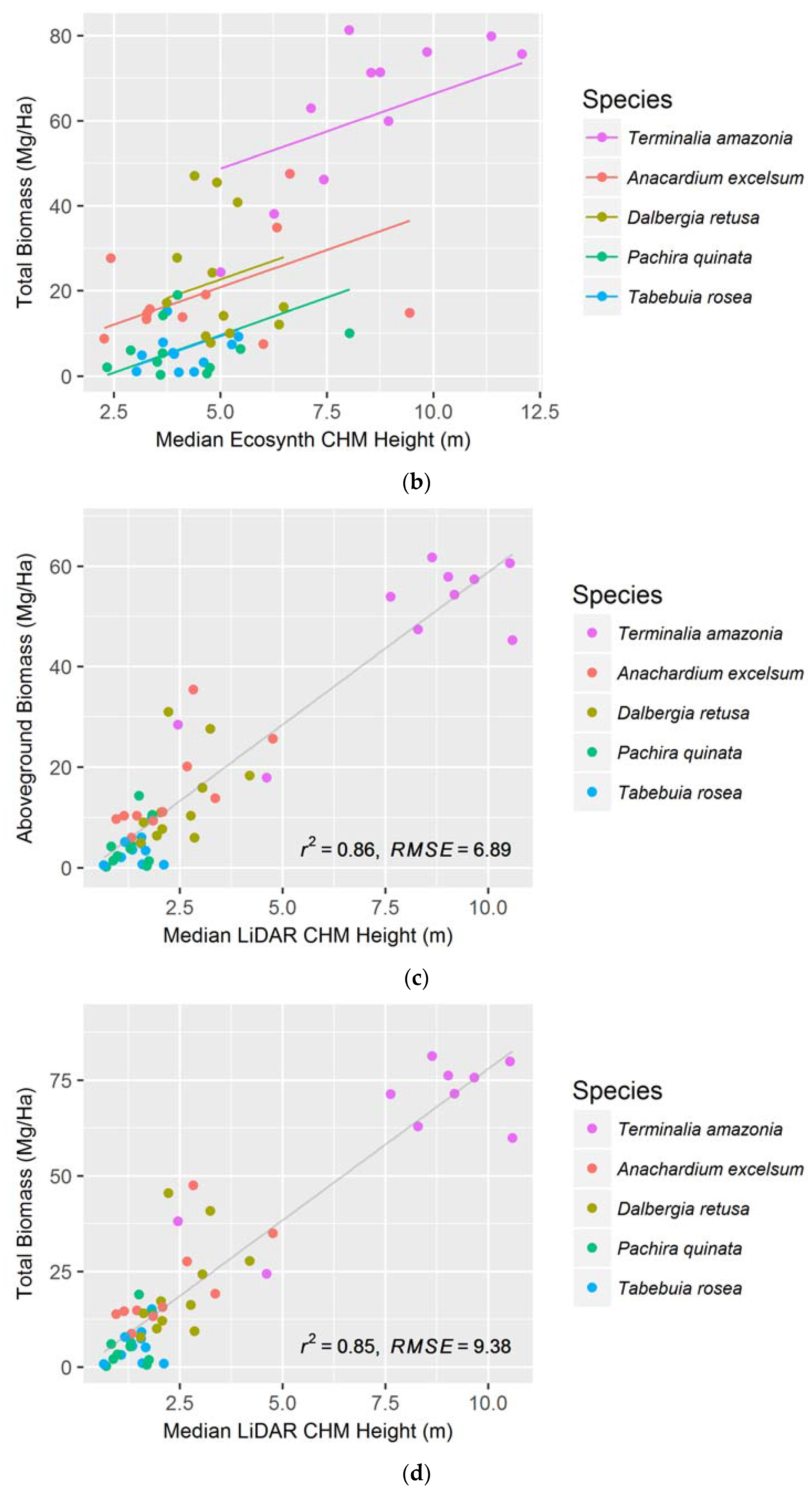
The median canopy height metric was the best predictor for both AGB and TB when examining the species together using the Ecosynth CHM. The strongest model was a linear mixed effect model that took species as the random effect and accounted for random y-intercepts (see Figure 4a,b). Using data from a LiDAR terrain model, via the LiDAR CHM, the median canopy height metric best models AGB and TB with a simple linear regression (AIC: 347.6 and 379.1 respectively, see Figure 4c,d). The LiDAR CHM improved the prediction of AGB and TB compared to the Ecosynth CHM (see Table 1).
When linear models were created to predict AGB and TB for individual species, we found that the optimal height metric depended on the species and terrain model. For the drone terrain model, AGB and TB of most species were best estimated with mean and 25 percentile height metrics, and for the LiDAR terrain model, maximum and median height metrics most accurately predicted biomass. The LiDAR CHM more accurately predicted AGB and TB for every species compared to the Ecosynth CHM; except for when modeling TB for T. amazonia (see Table 2). Unlike the height models, the species-specific biomass regressions from drone and LiDAR data did not exhibit the same order of predictive ability (see Table 2).
3.3. Vertical Canopy Profiles
The vertical canopy profiles correctly capture the distinction in vertical stature between species but the LiDAR profiles better reflect the known vertical structure distribution of the species. This was determined by comparing the mean heights from the profiles of the different species to the mean heights of each species from the field data (see Figure 5a,b). For every species except for T. amazonia, the Ecosynth CHM profile overestimated field height while the LiDAR CHM provided a much closer approximation to field height.
4. Discussion
As expected, drone-derived point clouds more accurately predicted canopy heights during the dry season when used with a LiDAR DTM than with an Ecosynth DTM. When surveying multiple species at a time, drone point clouds, combined with LiDAR DTM, can predict plot-level height comparably to what has been measured with LiDAR point clouds and LiDAR DTMs [37,40]. Comparing the species-specific height models demonstrates that while the LiDAR CHM more accurately predicts height for all species than the Ecosynth CHM, both CHMs demonstrate the same order of predictive ability (see Table 1). Height of T. amazonia and D. retusa were predicted most accurately—with the T. amazonia models performing significantly better than any other, regardless of which terrain model was used.
In terms of biomass, the LiDAR CHM more accurately predicted AGB and TB than the Ecosynth CHM for every species except for T. amazonia. The LiDAR CHM most strongly predicted A. excelsum while the Ecosynth CHM most strongly predicted T. amazonia. The species with the lowest predictive ability for AGB and TB for both models were D. retusa and P. quinata. The results also demonstrate that the Ecosynth CHM and the LiDAR CHM could predict TB with nearly identical regression coefficients to AGB models. This is an important step in carbon measurement studies because many remote sensing studies up to this point have focused primarily on AGB, disregarding a significant portion of a forest’s carbon—that which is below ground [9,41,42,43,44,45,46]. By incorporating belowground biomass into calculations, we can produce more accurate carbon estimates, and with the aid of drones, do so faster and cheaper in monoculture plantations.
Both the species-specific height and biomass models demonstrate a significant difference in predictive ability between species. The Ecosynth CHM and LiDAR CHM most accurately predicted height and biomass for T. amazonia and A. excelsum, and least accurately predicted both metrics for D. retusa, T. rosea, and P. quinata. The two species with the most accurate models are both single-stemmed evergreen trees while the other three are deciduous, and one of them is multi-stemmed. These results suggest that in the steepland tropics, drone point clouds can be used to accurately measure the plot-level height of tall evergreen trees but not small deciduous ones during the dry season. This difference is likely because the structure from motion algorithms is not as effective when the drone photos contain less visible features (i.e., leaves) to identify. While other researchers have shown a distinction between leaf-on and leaf-off drone accuracy [22], this is the first study to isolate the experiments on a per-species basis using tropical timber species. This is important because many plantations in the tropics are either subdivided into mono-specific patches or are entirely monocultures [47].
In every case, the LiDAR CHM produced more accurate models than the Ecosynth CHM, although the Ecosynth CHM acceptably predicted height and biomass for certain species. The most likely explanation for this discrepancy is the terrain-filtering algorithm which is used to create the Ecosynth CHM. The point cloud creation and terrain filtering processes both work best on flat ground and in areas with visible terrain [21,48,49]. In this study, many areas of the terrain were covered by ground vegetation, likely causing elevation overestimation and a source of error in both the Ecosynth and LiDAR terrain filtering algorithms [39]. As described elsewhere, accuracy can be improved by placing ground control markers, such as bright targets, to be referenced in the drone imagery [18]. In the steepland tropics, for future studies, we recommend either using ground control markers, LiDAR-derived terrain models, or GPS-based terrain models.
5. Conclusions
Data collected by drones, when used with accurate terrain models, can accurately measure biomass and heights of select species in monoculture plantations. Because they are small and easy-to-operate, drones can be used in hard-to-reach locations as a field tool in mapping and monitoring plantation growth, given the right species and time of year. Because of their low cost and potential for rapid deployment, drones overcome the cost and time barriers often associated with LiDAR and field inventories. However, as we have shown, drone measurements must be used in conjunction with field-derived biomass equations, high accuracy terrain models, and GPS data collected from the field to improve survey accuracy.
Canopy height metrics from drone measurements, regardless of the DTM used, can predict total biomass as well as aboveground biomass. This finding opens the door to further research into drone-based total biomass estimation, a metric that has too often been overlooked by biomass studies. Accurately calculating both above and belowground biomass of plantations and forests is a critical step in improving local and national carbon budgets.
This study also demonstrates that drone point cloud data can be used with LiDAR terrain models to acquire accurate models of height and biomass for select species. In places where LiDAR terrain models are already available, drones can be used to cost-effectively re-survey plantation growth and biomass accumulation.
While Ecosynth shows promise for plantation assessments, it has its limitations. The Ecosynth methodology requires a high degree of skill to process the data. New user-friendly applications though, such as ESRI’s Drone2Map (ESRI, Redlands, CA, USA) are lowering this barrier to entry. Additionally, variables such as wind, light, and camera settings can change the quality of the data (see [25] for an outline of optimal conditions).
Drones, especially when used with existing DTMs, can accurately measure monoculture plantation heights but their ability to characterize all species’ heights and biomass in tropical steeplands depends on phenology, architecture, and terrain variability. The methodology can be employed rapidly and holds great promise for measuring small-scale plantations. To realize the full potential of drones, researchers should continue to test the limitations of the technology. These studies will allow resource managers to make informed decisions about the use of this technology and identify areas for future research and development. With continued study, drones can be used to deliver a degree of timeliness and cost-efficiency to plantation assessments not seen before in forestry.
Supplementary Materials
The following are available online at www.mdpi.com/1999-4907/8/5/168/s1.
Acknowledgments
This work is a contribution of the Agua Salud Project and the Smart Reforestation® program of the Smithsonian Tropical Research Institute (STRI). Agua Salud is part of ForestGEO and is a collaboration with the Panama Canal Authority, the Ministry of the Environment of Panama, and other partners. Research funding for this work came from Stanley Motta, the Silicon Valley Foundation, the Heising-Simons Foundation and the National Science Foundation grant (NSF grant EAR-1360391). Data processing was funded by a STRI Short-Term Fellowship, awarded to Ethan Miller. We thank Marino Ramírez for assistance with the drone data collection, Milton Solano for his work with the data preparation and organization, and the many staff at the Smithsonian Tropical Research Institute who made field work possible—primarily Frederico Davies. We also thank the many technicians and workers who have tended the Agua Salud plantations over the last few years, and especially those who conducted the inventories.
Author Contributions
E.M. and J.S.H. conceived and designed the research idea; J.P.D. collected the drone data, performed initial image processing, and wrote cover letter; E.M. and M.D. analyzed the data; J.S.H. contributed inventory data, oversaw field work; E.M. wrote the paper, all authors provided comments and reviewed paper.
Conflicts of Interest
The authors declare no conflict of interest. The founding sponsors had no role in the design of the study; in the collection, analyses, or interpretation of data; in the writing of the manuscript, and in the decision to publish the results.
References
- Jürgensen, C.; Kollert, W.; Lebedys, A. Assessment of Industrial Roundwood Production from Planted Forests. FAO Planted Forests and Trees Working Paper FP/48/E. Rome, 2014. Available online: http://www.fao.org/forestry/plantedforests/67508@170537/en/ (accessed on 30 March 2017).
- Hall, J.S.; Ashton, M.S.; Garen, E.J.; Jose, S. The ecology and ecosystem services of native trees: Implications for reforestation and land restoration in Mesoamerica. For. Ecol. Manag. 2011, 261, 1553–1557. [Google Scholar] [CrossRef]
- Understanding Relationships between Biodiversity, Carbon, Forests and People: The Key to Achieving REDD+ Objectives. A Global Assessment Report Prepared by the Global Forest Expert Panel on Biodiversity, Forest Management and REDD+. Available online: https://www.google.ch/url?sa=t&rct=j&q=&esrc=s&source=web&cd=1&cad=rja&uact=8&ved=0ahUKEwjyxfa79OHTAhVpJcAKHermBPoQFggiMAA&url=http%3A%2F%2Fwww.iufro.org%2Fdownload%2Ffile%2F18866%2F5303%2Fws31_pdf%2F&usg=AFQjCNFgUfIhHKJklsRP2IOp2578WDoeXw (accessed on 9 May 2017).
- Pawson, S.M.; Brin, A.; Brockerhoff, E.G.; Lamb, D.; Payn, T.W.; Paquette, A.; Parrotta, J.A. Plantation forests, climate change and biodiversity. Biodivers. Conserv. 2013, 22, 1203–1227. [Google Scholar] [CrossRef]
- Edwards, D.P.; Fisher, B.; Boyd, E. Protecting degraded rainforests: Enhancement of forest carbon stocks under REDD+. Conserv. Lett. 2010, 3, 313–316. [Google Scholar] [CrossRef]
- Van Breugel, M.; Ransijn, J.; Craven, D.; Bongers, F.; Hall, J.S. Estimating carbon stock in secondary forests: Decisions and uncertainties associated with allometric biomass models. For. Ecol. Manag. 2011, 262, 1648–1657. [Google Scholar] [CrossRef]
- Chave, J.; Andalo, C.; Brown, S.; Cairns, M.A.; Chambers, J.Q.; Eamus, D.; Fölster, H.; Fromard, F.; Higuchi, N.; Kira, T.; et al. Tree allometry and improved estimation of carbon stocks and balance in tropical forests. Oecologia 2005, 145, 87–99. [Google Scholar] [CrossRef] [PubMed]
- De Sy, V.; Herold, M.; Achard, F.; Asner, G.P.; Held, A.; Kellndorfer, J.; Verbesselt, J. Synergies of multiple remote sensing data sources for REDD+ monitoring. Curr. Opin. Environ. Sustain. 2012, 4, 696–706. [Google Scholar] [CrossRef]
- Asner, G.P.; Mascaro, J.; Muller-Landau, H.C.; Vieilledent, G.; Vaudry, R.; Rasamoelina, M.; Hall, J.S.; van Breugel, M. A universal airborne LiDAR approach for tropical forest carbon mapping. Oecologia 2012, 168, 1147–1160. [Google Scholar] [CrossRef] [PubMed]
- Van Leeuwen, M.; Nieuwenhuis, M. Retrieval of forest structural parameters using LiDAR remote sensing. Eur. J. For. Res. 2010, 129, 749–770. [Google Scholar] [CrossRef]
- Hunter, M.O.; Keller, M.; Victoria, D.; Morton, D.C. Tree height and tropical forest biomass estimation. Biogeosciences 2013, 10, 8385–8399. [Google Scholar] [CrossRef]
- Omasa, K.; Hosoi, F.; Konishi, A. 3D lidar imaging for detecting and understanding plant responses and canopy structure. J. Exp. Bot. 2007, 58, 881–898. [Google Scholar] [CrossRef] [PubMed]
- Silva, C.A.; Klauberg, C.; Pádua, S.de.; Hudak, A.T.; Rodriguez, L.C. Mapping aboveground carbon stocks using LiDAR data in Eucalyptus spp. plantations in the state of São Paulo, Brazil. Sci. For. 2014, 42, 591–604. [Google Scholar]
- Detto, M.; Asner, G.P.; Muller-Landau, H.C.; Sonnentag, O. Spatial variability in tropical forest leaf area density from Multireturn LiDAR and modelling. J. Geophys. Res. Biogeosciences 2015, 1–16. [Google Scholar] [CrossRef]
- Erdody, T.L.; Moskal, L.M. Fusion of LiDAR and imagery for estimating forest canopy fuels. Remote Sens. Environ. 2010, 114, 725–737. [Google Scholar] [CrossRef]
- Anderson, K.; Gaston, K.J. Lightweight unmanned aerial vehicles will revolutionize spatial ecology. Front. Ecol. Environ. 2013, 11, 138–146. [Google Scholar] [CrossRef]
- Koh, L.P.; Wich, S.A. Dawn of drone ecology: Low-Cost autonomous aerial vehicles for conservation. Trop. Conserv. Sci. 2012, 5, 121–132. [Google Scholar] [CrossRef]
- Zahawi, R.A.; Dandois, J.P.; Holl, K.D.; Nadwodny, D.; Reid, J.L.; Ellis, E.C. Using lightweight unmanned aerial vehicles to monitor tropical forest recovery. Biol. Conserv. 2015, 186, 287–295. [Google Scholar] [CrossRef]
- Wundram, D.; Löffler, J. High-resolution spatial analysis of mountain landscapes using a low-altitude remote sensing approach. Int. J. Remote Sens. 2008, 29, 961–974. [Google Scholar] [CrossRef]
- Rango, A.; Laliberte, A.; Herrick, J.E.; Winters, C.; Havstad, K.; Steele, C.; Browning, D. Unmanned aerial vehicle-based remote sensing for rangeland assessment, monitoring, and management. J. Appl. Remote Sens. 2009, 3, 1–15. [Google Scholar]
- Dandois, J.P.; Ellis, E.C. High spatial resolution three-dimensional mapping of vegetation spectral dynamics using computer vision. Remote Sens. Environ. 2013, 136, 259–276. [Google Scholar] [CrossRef]
- Dandois, J.P.; Ellis, E.C. Remote sensing of vegetation structure using computer vision. Remote Sens. 2010, 2, 1157–1176. [Google Scholar] [CrossRef]
- Triggs, B.; McLauchlan, P.F.; Hartley, R.I.; Fitzgibbon, A.W. Bundle Adjustment—A Modern Synthesis. Vis. Algorithms Theory Pract. 2000, 1883, 298–372. [Google Scholar]
- Snavely, N.; Seitz, S.M.; Szeliski, R. Modeling the world from Internet photo collections. Int. J. Comput. Vis. 2008, 80, 189–210. [Google Scholar] [CrossRef]
- Dandois, J.P.; Olano, M.; Ellis, E.C. Optimal altitude, overlap, and weather conditions for computer vision UAV estimates of forest structure. Remote Sens. 2015, 7, 13895–13920. [Google Scholar] [CrossRef]
- Shaxson, F. New Concepts and Approaches to Land Management in the Tropics with Emphasis on Steeplands; FAO Soils Bulletin 75; Food and Agriculture Organization of the United Nations: Rome, Italy, 1999. [Google Scholar]
- Hall, J.S.; Love, B.E.; Garen, E.J.; Slusser, J.L.; Saltonstall, K.; Mathias, S.; van Breugel, M.; Ibarra, D.; Bork, E.W.; Spaner, D.; et al. Tree plantations on farms: Evaluating growth and potential for success. For. Ecol. Manag. 2011, 261, 1675–1683. [Google Scholar] [CrossRef]
- Hall, J.S.; Moss, D.; Stallard, R.F.; Raes, L.; Balvanera, P.; Asbjornsen, H.; Murgueitio, E.; Calle, Z.; Slusser, J.; Kirn, V.; et al. Managing Watersheds for Ecosystem Services in the Steepland Neotropics; Hall, J.S., Kirn, V., Yanguas-Fernandez, E., Eds.; Inter-American Development Bank: Panama City, Panama, 2015. [Google Scholar]
- Hartemink, A.E. Plantation agriculture in the tropics: Environmental issues. Outlook Agric. 2005, 34, 11–21. [Google Scholar] [CrossRef]
- Lisein, J.; Pierrot-Deseilligny, M.; Bonnet, S.; Lejeune, P. A Photogrammetric Workflow for the Creation of a Forest Canopy Height Model from Small Unmanned Aerial System Imagery. Forests 2013, 4, 922–944. [Google Scholar] [CrossRef]
- Felderhof, L.; Gillieson, D. Near-infrared imagery from unmanned aerial systems and satellites can be used to specify fertilizer application rates in tree crops. Can. J. Remote Sens. 2012, 37, 376–386. [Google Scholar] [CrossRef]
- Tang, L.; Shao, G. Drone remote sensing for forestry research and practices. J. For. Res. 2015, 26, 791–797. [Google Scholar] [CrossRef]
- Ogden, F.L.; Crouch, T.D.; Stallard, R.F.; Hall, J.S. Effect of land cover and use on dry season river runoff, runoff efficiency, and peak storm runoff in the seasonal tropics of Central Panama. Water Resour. Res. 2013, 49, 8443–8462. [Google Scholar] [CrossRef]
- Van Breugel, M.; Hall, J.S.; Craven, D.; Bailon, M.; Hernandez, A.; Abbene, M.; van Breugel, P. Succession of ephemeral secondary forests and their limited role for the conservation of floristic diversity in a human-modified tropical landscape. PLoS ONE 2013, 8. [Google Scholar] [CrossRef] [PubMed]
- Van Breugel, M.; Hall, J.S. Experimental Design of the “Agua Salud” Native Timber Species Plantation. Center for Tropical Forest Science, Smithsonian Institution, 2008. Typescript Report. Available online: http://www.ctfs.si.edu/aguasalud/page/documents/ (accessed on 4 February 2017).
- Sinacore, K.; Hall, J.S.; Potvin, C.; Royo, A.A.; Ducey, M.J.; Ashton, M.S. Competing belowground: Root biomass is an important factor toward better estimates of biomass accumulation in tropical plantations. PLoS ONE 2017, submitted. [Google Scholar]
- Lesky, M.A.; Cohen, W.B.; Parker, G.G.; Harding, D.J. Lidar remote sensing for ecosystem studies. Bioscience 2002, 52, 19–30. [Google Scholar] [CrossRef]
- Helmer, E.H.; Ruefenacht, B. Cloud-free satellite image mosaics with regression trees and histrogram matching. Photogramm. Eng. Remote Sens. 2005, 71, 1079–1089. [Google Scholar] [CrossRef]
- Evans, J.S.; Hudak, A.T. A multiscale curvature algorithm for classifying discrete return LiDAR in forested environments. Geosci. Rem. Sens. IEEE Trans. 2007, 45, 1029–1038. [Google Scholar] [CrossRef]
- Andersen, H.-E.; Reutebuch, S.E.; McGaughey, R.J. A rigorous assessment of tree height measurements obtained using airborne lidar and conventional field methods. Can. J. Remote Sens. 2006, 32, 355–366. [Google Scholar] [CrossRef]
- Patenaude, G.; Hill, R.A.; Milne, R.; Gaveau, D.L.A.; Briggs, B.B.J.; Dawson, T.P. Quantifying forest above ground carbon content using LiDAR remote sensing. Remote Sens. Environ. 2004, 93, 368–380. [Google Scholar] [CrossRef]
- Lefsky, M.A.; Cohen, W.B.; Harding, D.J.; Parker, G.G.; Acker, S.A.; Gower, S.T. Lidar remote sensing of above-ground biomass in three biomes. Global Ecol. Biogeogr. 2002, 11, 393–399. [Google Scholar] [CrossRef]
- Næsset, E.; Gobakken, T. Estimation of above- and below-ground biomass across regions of the boreal forest zone using airborne laser. Remote Sens. Environ. 2008, 112, 3079–3090. [Google Scholar] [CrossRef]
- Clark, M.L.; Roberts, D.A.; Ewel, J.J.; Clark, D.B. Estimation of tropical rain forest aboveground biomass With small-footprint lidar and hyperspectral sensors. Remote Sens. Environ. 2011, 115, 2931–2942. [Google Scholar] [CrossRef]
- He, Q.; Chen, E.; An, R.; Li, Y. Above-ground biomass and biomass components estimation using LiDAR data in a coniferous forest. Forests 2013, 4, 984–1002. [Google Scholar] [CrossRef]
- Ota, T.; Ogawa, M.; Shimizu, K.; Kajisa, T.; Mizoue, N.; Yoshida, S.; Takao, G.; Hirata, Y.; Furuya, N.; Sano, T.; et al. Aboveground biomass estimation using structure from motion approach with aerial photographs in a seasonal tropical forest. Forests 2015, 6, 3882–3898. [Google Scholar] [CrossRef]
- Nichols, J.D.; Bristow, M.; Vanclay, J.K. Mixed-species plantations: Prospects and challenges. For. Ecol. Manage. 2006, 233, 383–390. [Google Scholar] [CrossRef]
- Baltsavias, E.; Gruen, A.; Eisenbeiss, H.; Zhang, L.; Waser, L.T. High-quality image matching and automated generation of 3D tree models. Int. J. Remote Sens. 2008, 29, 1243–1259. [Google Scholar] [CrossRef]
- White, J.C.; Wulder, M.A.; Vastaranta, M.; Coops, N.C.; Pitt, D.; Woods, M. The utility of image-based point clouds for forest inventory: A comparison with airborne laser scanning. Forests 2013, 4, 518–536. [Google Scholar] [CrossRef]
Figure 1.
(a) Agua Salud study site, plots, and blocks locations; and (b) example of field plot.
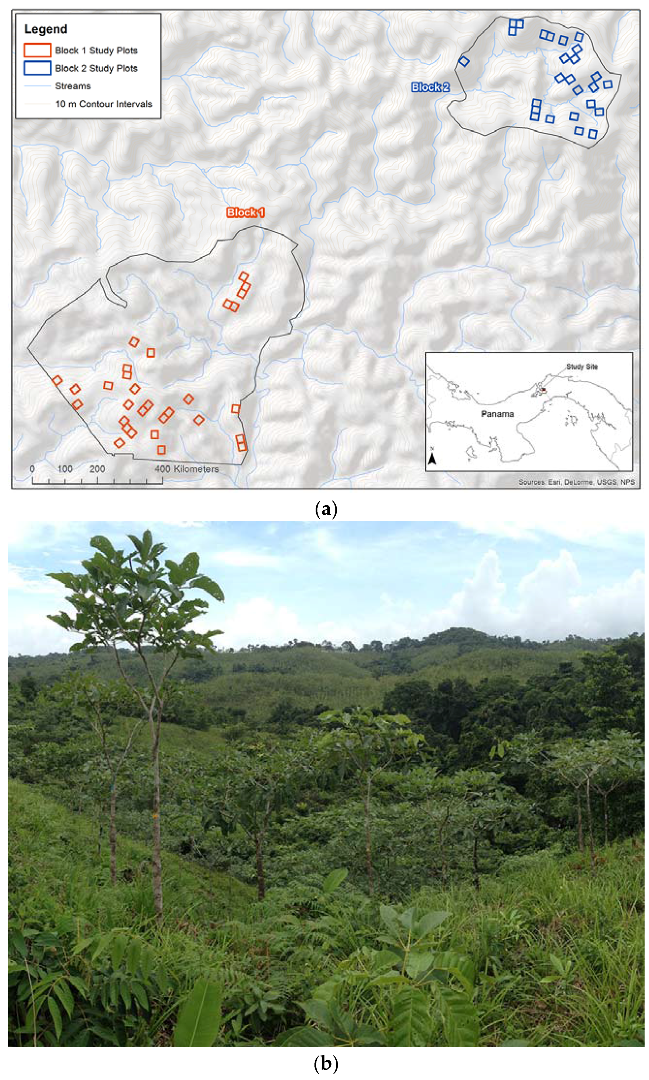
Figure 2.
Ecosynth canopy height model with manual canopy delineations of three plots.
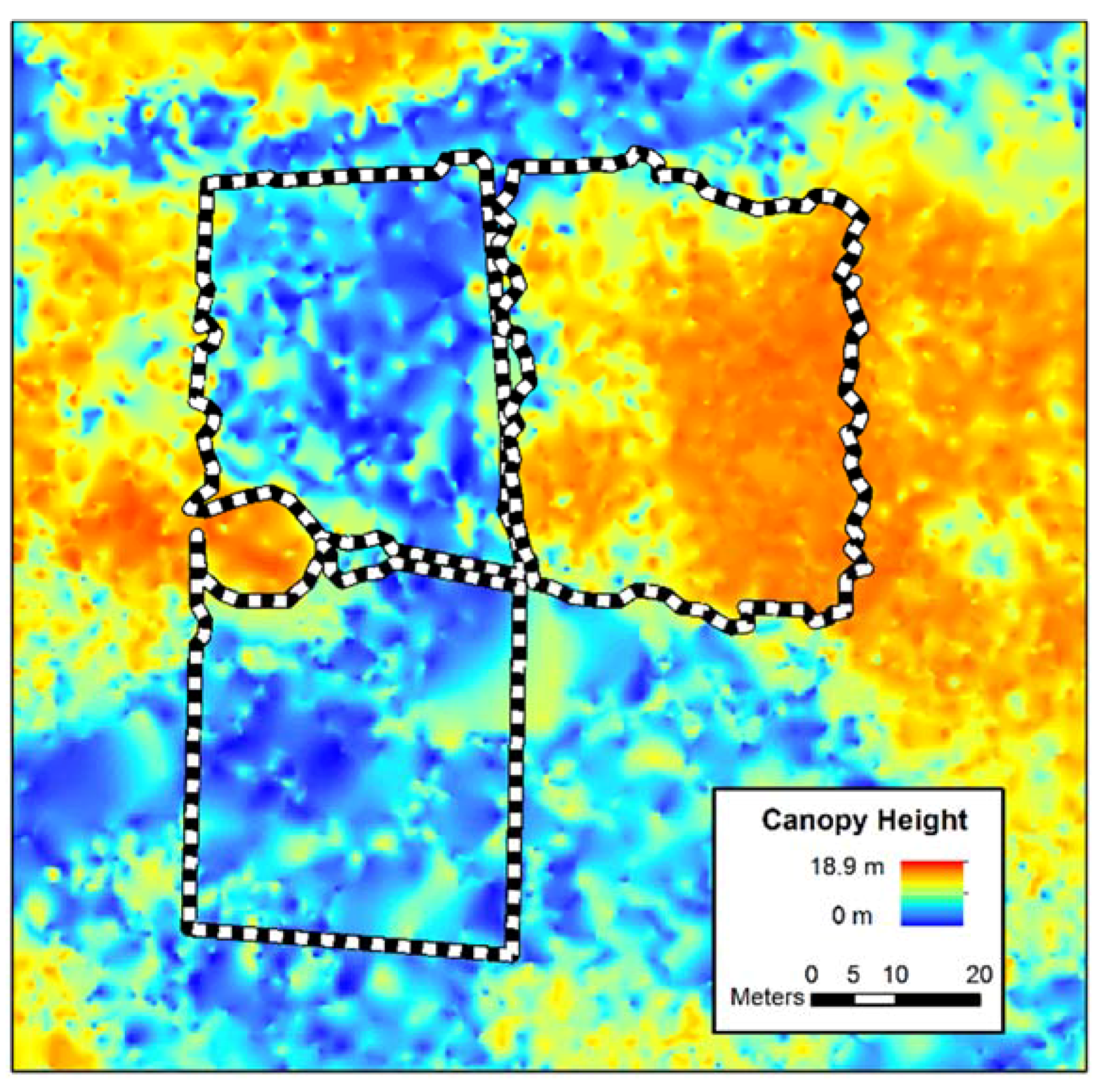
Figure 3.
(a) Median Ecosynth CHM, using the linear mixed effect model with random slopes; and (b) LiDAR CHM canopy height metrics, with simple linear regression, as predictors of plot-level mean field height (see Table 1 for model AICs). Points represent individual plots.
Figure 3.
(a) Median Ecosynth CHM, using the linear mixed effect model with random slopes; and (b) LiDAR CHM canopy height metrics, with simple linear regression, as predictors of plot-level mean field height (see Table 1 for model AICs). Points represent individual plots.
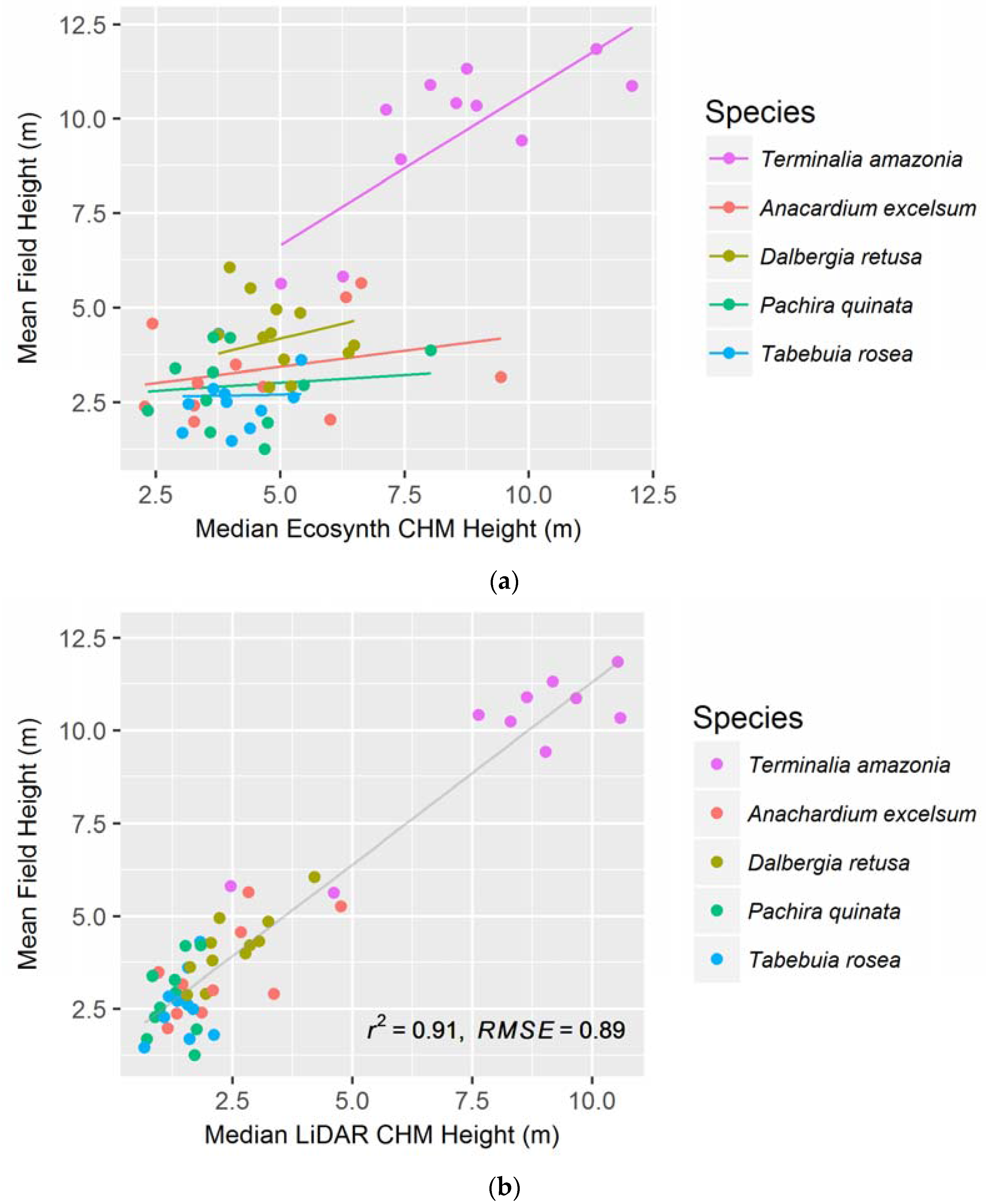
Figure 4.
Median Ecosynth CHM canopy height metrics as predictors of (a) aboveground biomass; and (b) total biomass using linear mixed effect modeling with random intercepts; Median LiDAR CHM canopy height metrics as predictors of (c) aboveground biomass; and (d) total biomass using simple linear regressions. See Table 1 for model AICs.


Figure 5.
Canopy height profiles of all treatments per species as determined by the (a) Ecosynth CHM; and (b) LiDAR CHM. The x-axis represents the fraction of points from the given CHM, and the plot demonstrates how those points are distributed vertically per species.
Figure 5.
Canopy height profiles of all treatments per species as determined by the (a) Ecosynth CHM; and (b) LiDAR CHM. The x-axis represents the fraction of points from the given CHM, and the plot demonstrates how those points are distributed vertically per species.

Table 1.
A comparison of Ecosynth and LiDAR canopy height models in their ability to predict field height, aboveground biomass (AGB), and total biomass (TB) for all treatments combined. The table shows which canopy metric and model were used and the models’ corresponding Akaike information criterion (AIC). LME stands for ‘Linear Mixed Effect’ and the type of LME used is designated.
| Ecosynth CHM | LiDAR CHM | |||||
|---|---|---|---|---|---|---|
| Height | AGB | TB | Height | AGB | TB | |
| Height Metric | Median | Median | Median | Median | Median | Median |
| Type of Model | LME—Random Slopes | LME—Random Intercepts | LME—Random Intercepts | Linear | Linear | Linear |
| AIC | 194.5 | 421.1 | 454.9 | 138.5 | 347.6 | 379.1 |
Table 2.
Results of comparisons between plot-level remotely-sensed height measurements and field-measured height, aboveground biomass, and total biomass of five species. Models were created with simple linear regressions. The R2 and RMSE values of each measurement are shown (R2/RMSE).
Table 2.
Results of comparisons between plot-level remotely-sensed height measurements and field-measured height, aboveground biomass, and total biomass of five species. Models were created with simple linear regressions. The R2 and RMSE values of each measurement are shown (R2/RMSE).
| Ecosynth CHM | LiDAR CHM | |||||
|---|---|---|---|---|---|---|
| Field Height | AGB | TB | Field Height | AGB | TB | |
| Height Metric | Median | In italics | In italics | Median | In italics | In italics |
| T. amazonia | 0.58 */1.29 | 0.64/8.24 * Median | 0.71/9.64 * 75 Percentile | 0.83/0.86 *** | 0.64/8.21 * Median | 0.65/10.6 * Median |
| D. retusa | 0.16/0.84 | 0.07/9.19 Mean | 0.07/13.3 Mean | 0.69/0.49 * | 0.24/7.37 Maximum | 0.24/10.6 Maximum |
| P. quinata | 0.03/0.95 | 0.06/4.14 25 Percentile | 0.06/5.47 25 Percentile | 0.04/0.94 | 0.16/4.03 Median | 0.15/5.33 Median |
| T. rosea | 0.05/0.77 | 0.03/2.64 25 Percentile | 0.03/4.01 25 Percentile | 0.10/0.79 | 0.40/2.18 Maximum | 0.40/3.31 * Maximum |
| A. excelsum | 0.09/1.16 | 0.03/8.65 25 Percentile | 0.03/11.4 25 Percentile | 0.45/0.89 * | 0.82/3.64 ** Maximum | 0.83/4.73 ** Maximum |
* p < 0.05, ** p < 0.001, *** p < 0.0001.
© 2017 by the authors. Licensee MDPI, Basel, Switzerland. This article is an open access article distributed under the terms and conditions of the Creative Commons Attribution (CC BY) license (http://creativecommons.org/licenses/by/4.0/).
Share and Cite
MDPI and ACS Style
Miller, E.; Dandois, J.P.; Detto, M.; Hall, J.S. Drones as a Tool for Monoculture Plantation Assessment in the Steepland Tropics. Forests 2017, 8, 168. https://doi.org/10.3390/f8050168
AMA Style
Miller E, Dandois JP, Detto M, Hall JS. Drones as a Tool for Monoculture Plantation Assessment in the Steepland Tropics. Forests. 2017; 8(5):168. https://doi.org/10.3390/f8050168
Chicago/Turabian StyleMiller, Ethan, Jonathan P. Dandois, Matteo Detto, and Jefferson S. Hall. 2017. "Drones as a Tool for Monoculture Plantation Assessment in the Steepland Tropics" Forests 8, no. 5: 168. https://doi.org/10.3390/f8050168
Note that from the first issue of 2016, this journal uses article numbers instead of page numbers. See further details here.