
Terrestrial Laser Scanning for Forest Inventories—Tree Diameter Distribution and Scanner Location Impact on Occlusion

 and
and
Abstract
:1. Introduction
- (i)
- To demonstrate the relationships between angular resolution of the scanner, object size, distance to the scanner and the possible sampling frequency (scanner point density) on an object with TLS in a 3D space. This should help determine the minimal object size detectable by TLS.
- (ii)
- To show the connection between the visibility of a sample plot and its stand describing parameters, such as diameter distribution, stem number and dominant diameter. This experiment improves the understanding of how the stand properties influence the scan quality. We hypothesize that there is a very strong link between the stand parameters and the visibility.
- (iii)
- To demonstrate the influence of the scanning location within a sample plot on the visibility.
- (iv)
- To understand the mechanism behind occlusion and to determine the most suitable scanner location patterns for TLS acquisitions in forests.
2. Materials and Methods
2.1. The NFI Framework, Data and Tools
2.1.1. Sample Plot
2.1.2. NFI Data
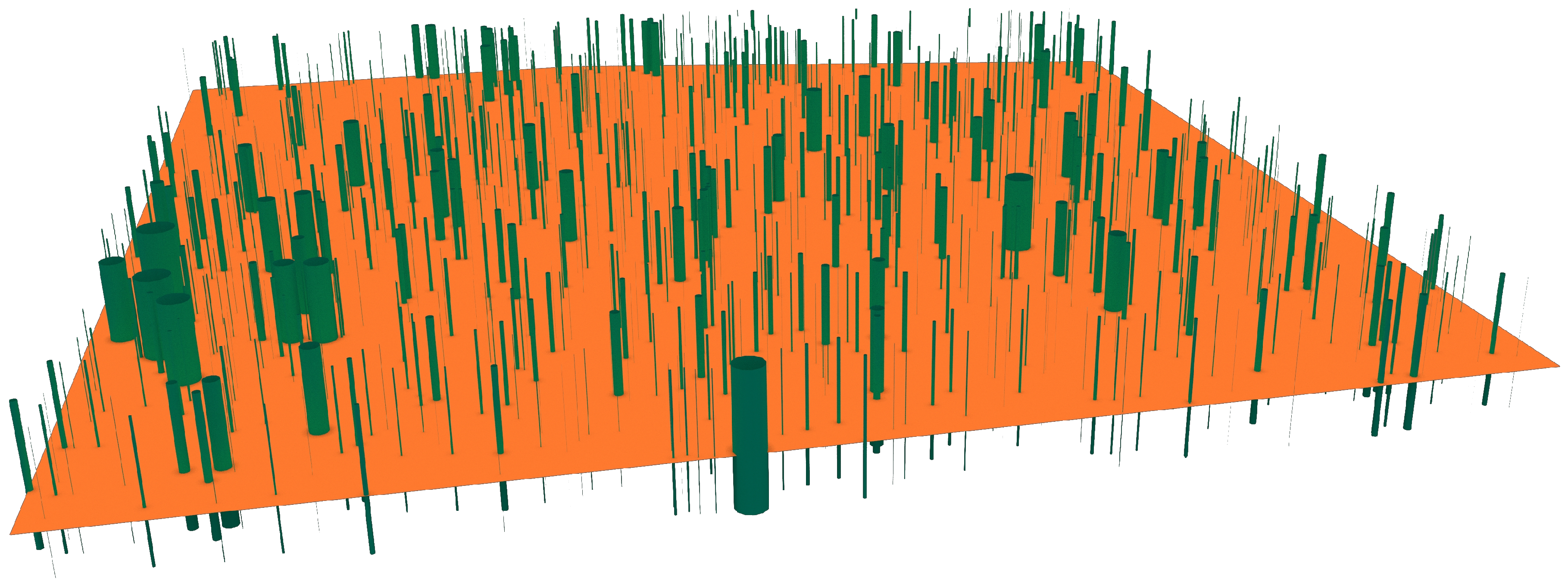
2.1.3. Blender
2.1.4. Simulated Laser Scanning
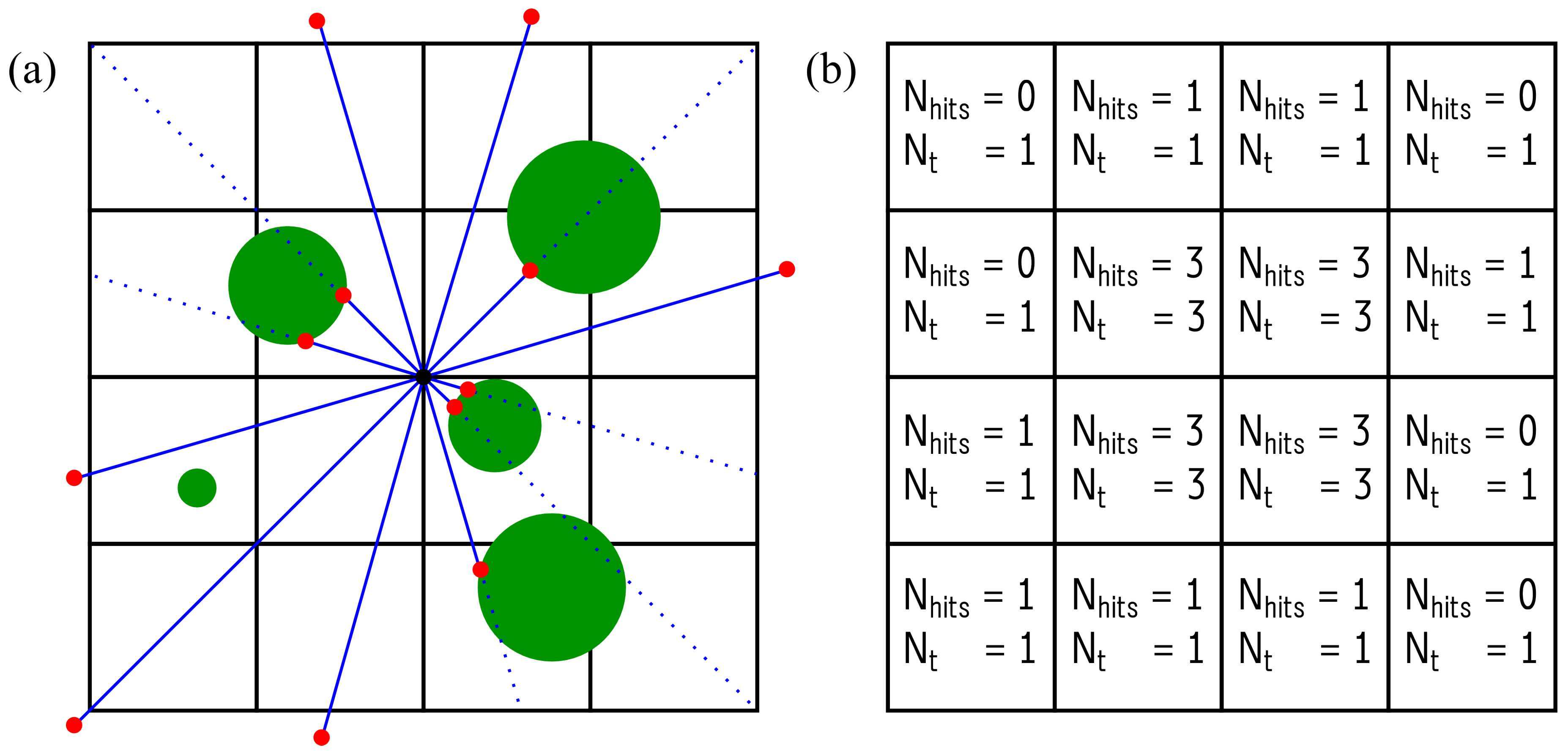
2.1.5. Voxel Traversal Algorithm
2.1.6. Visibility Assessment
2.2. Theoretical Coverage of a Laser Scanning System in a 3D Space
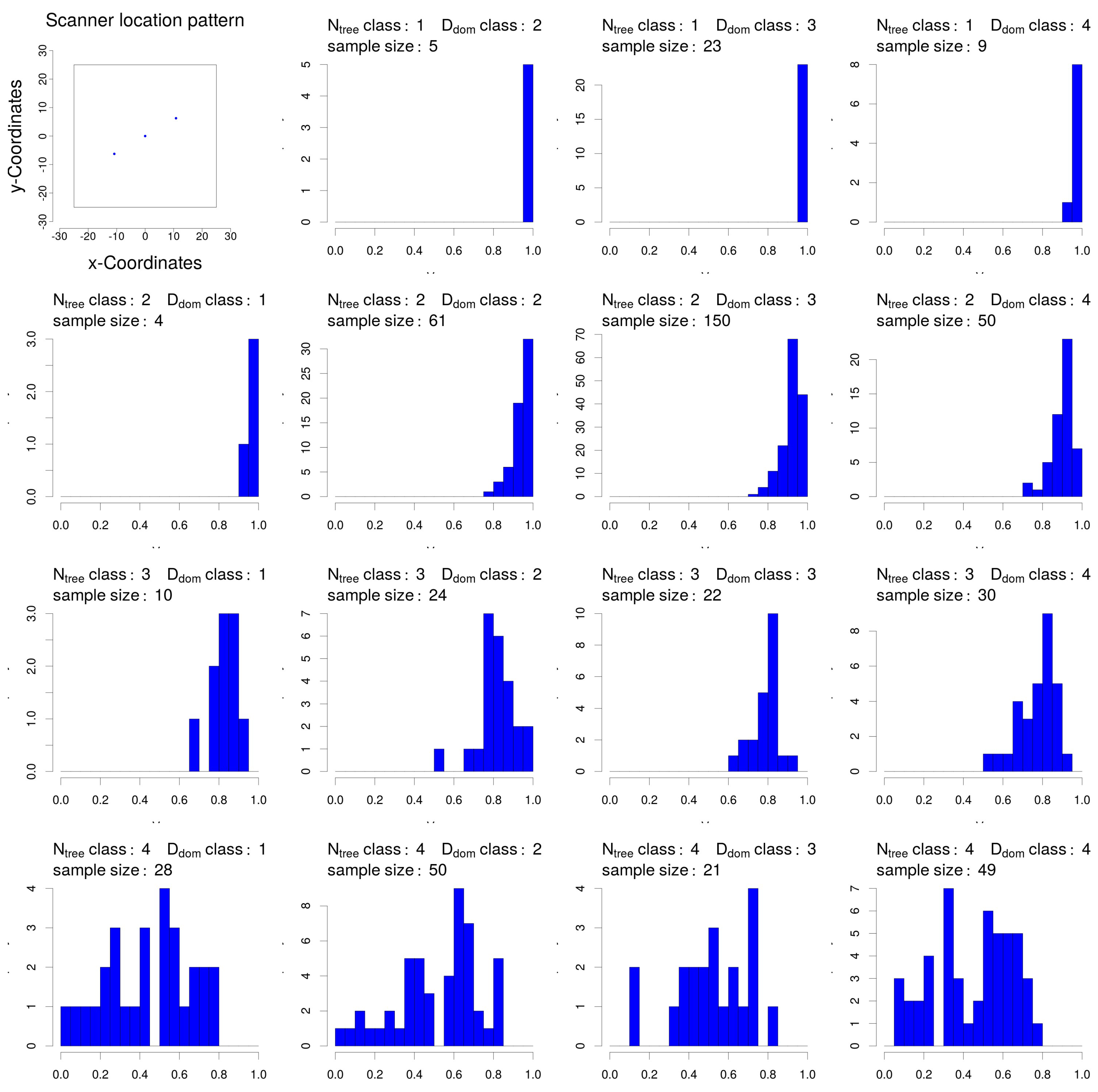
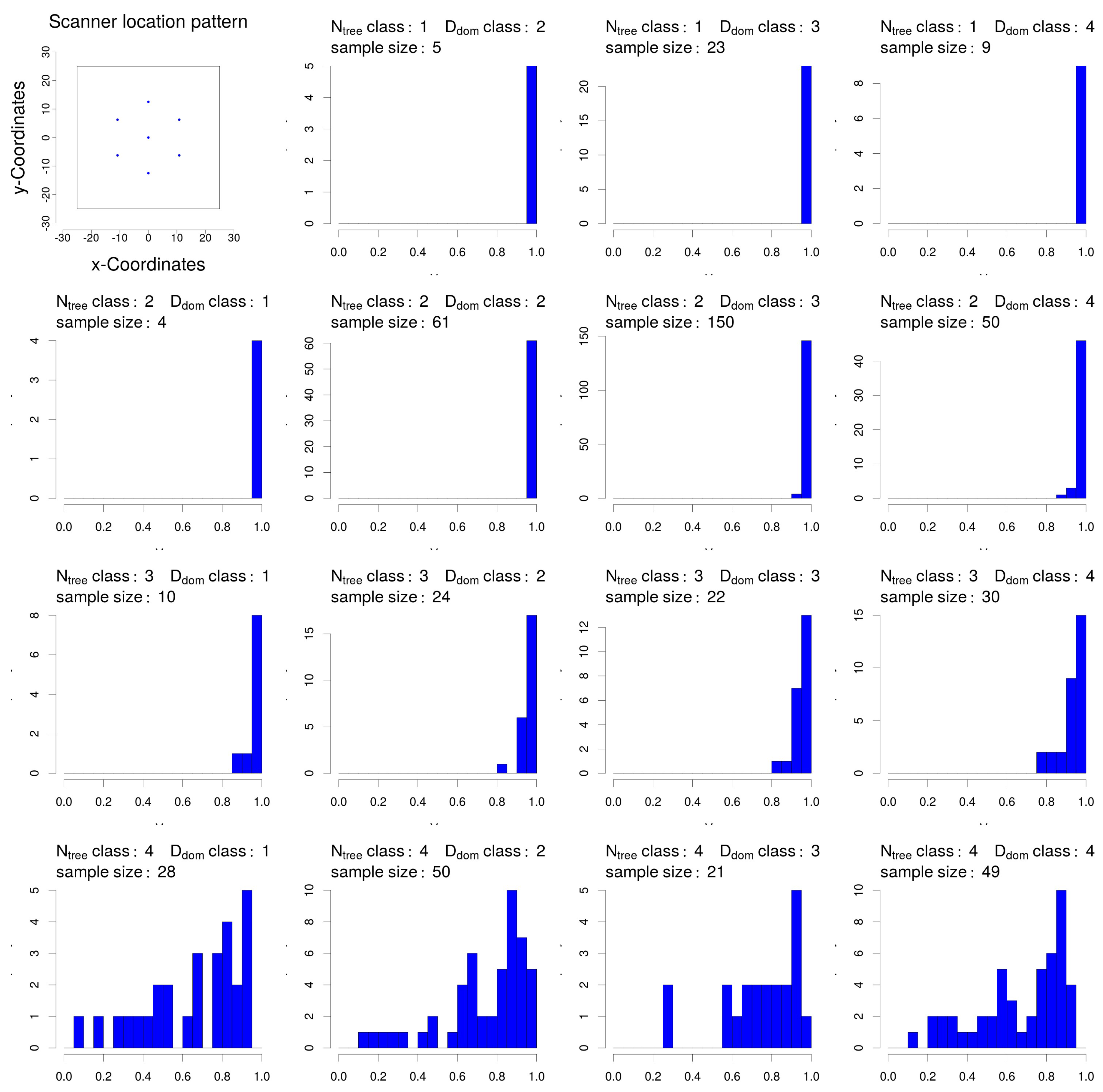
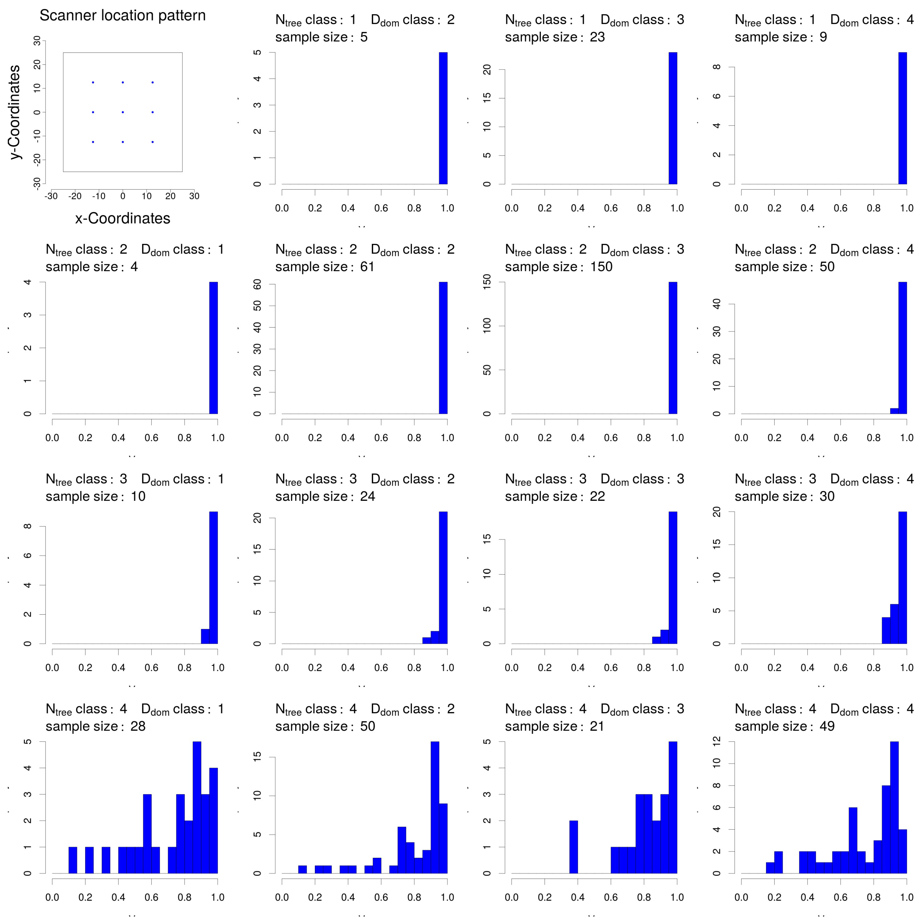
2.3. Influence of Stand Parameters on Visibility in a 2D Space
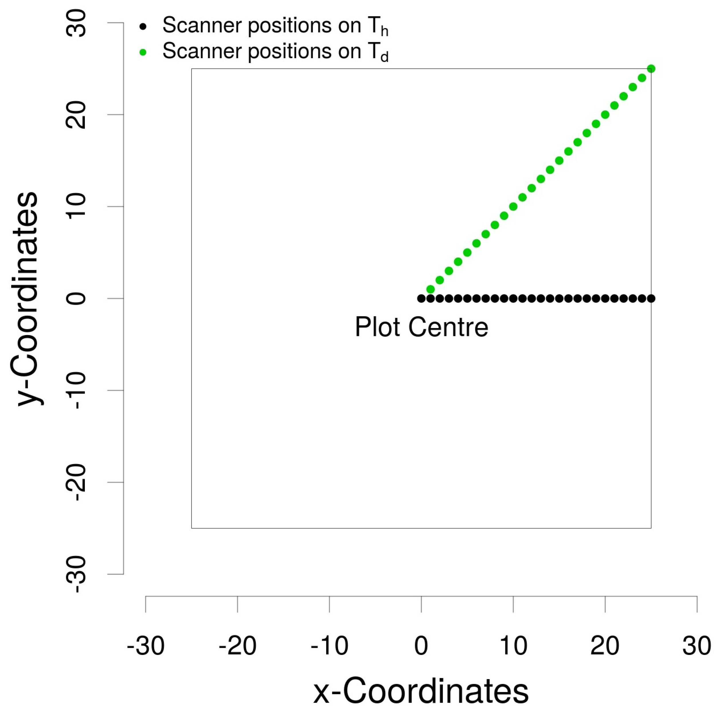
2.4. Influence of the Scanning Location within Sample Plots on Visibility in a 2D Space
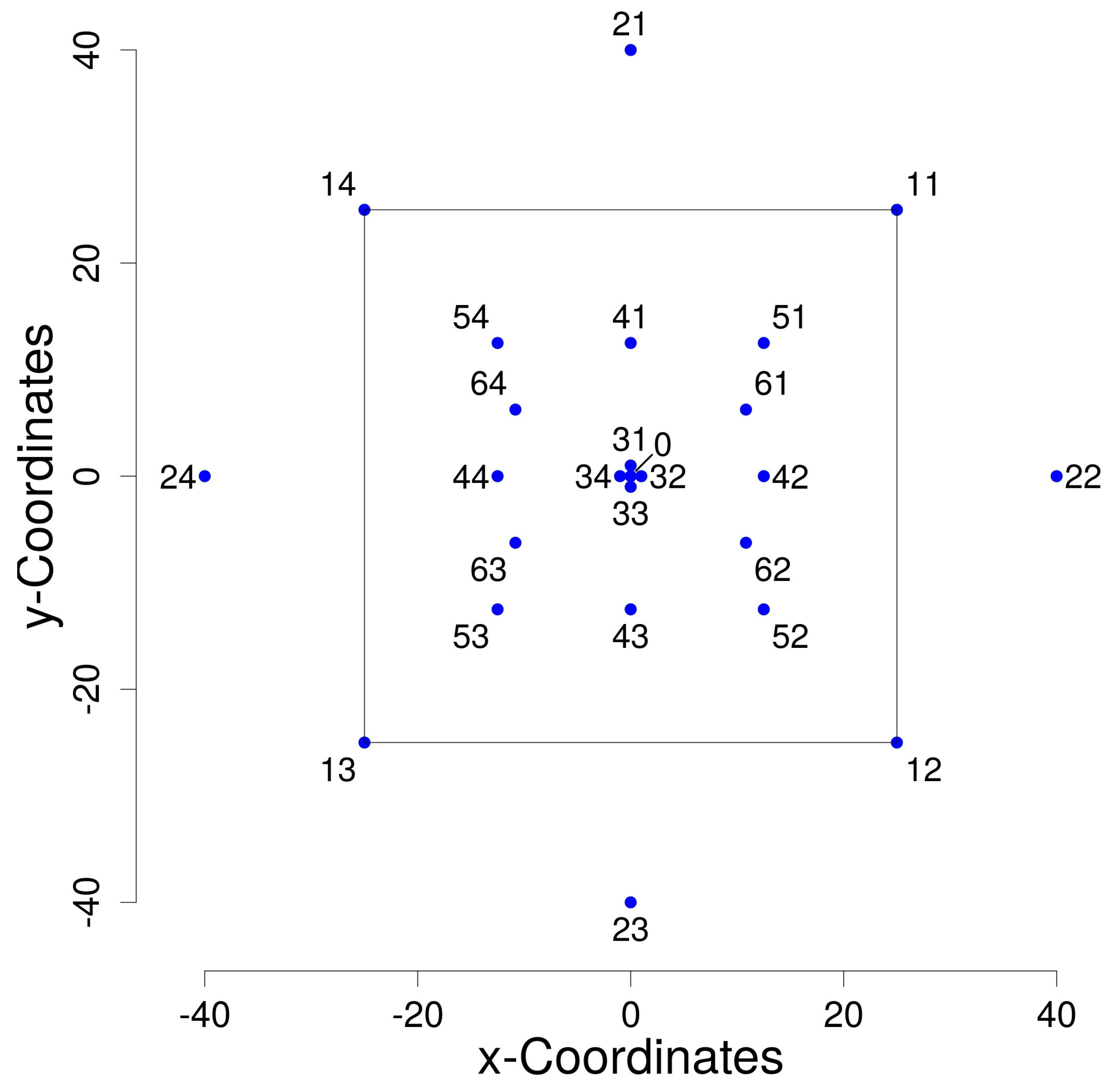
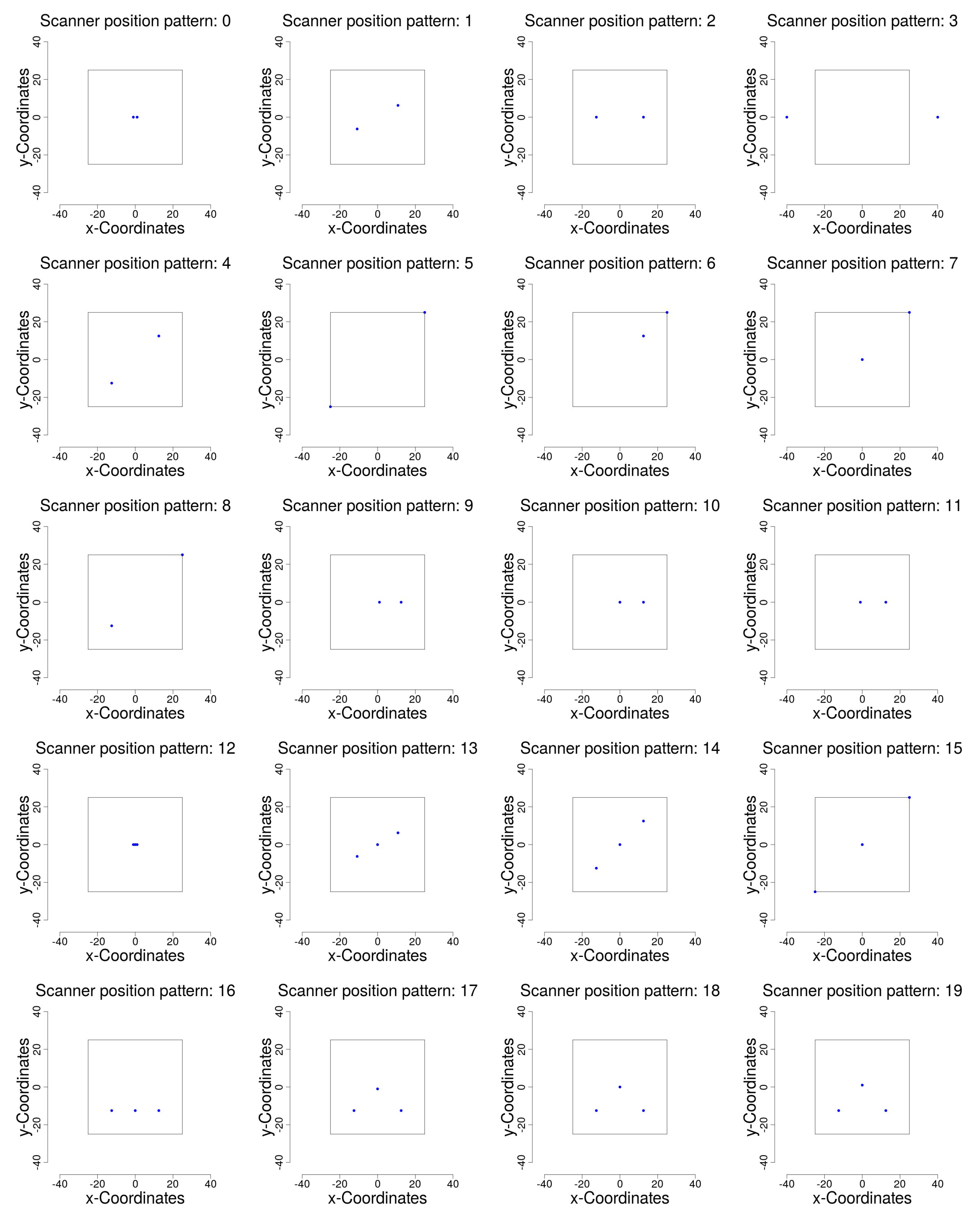
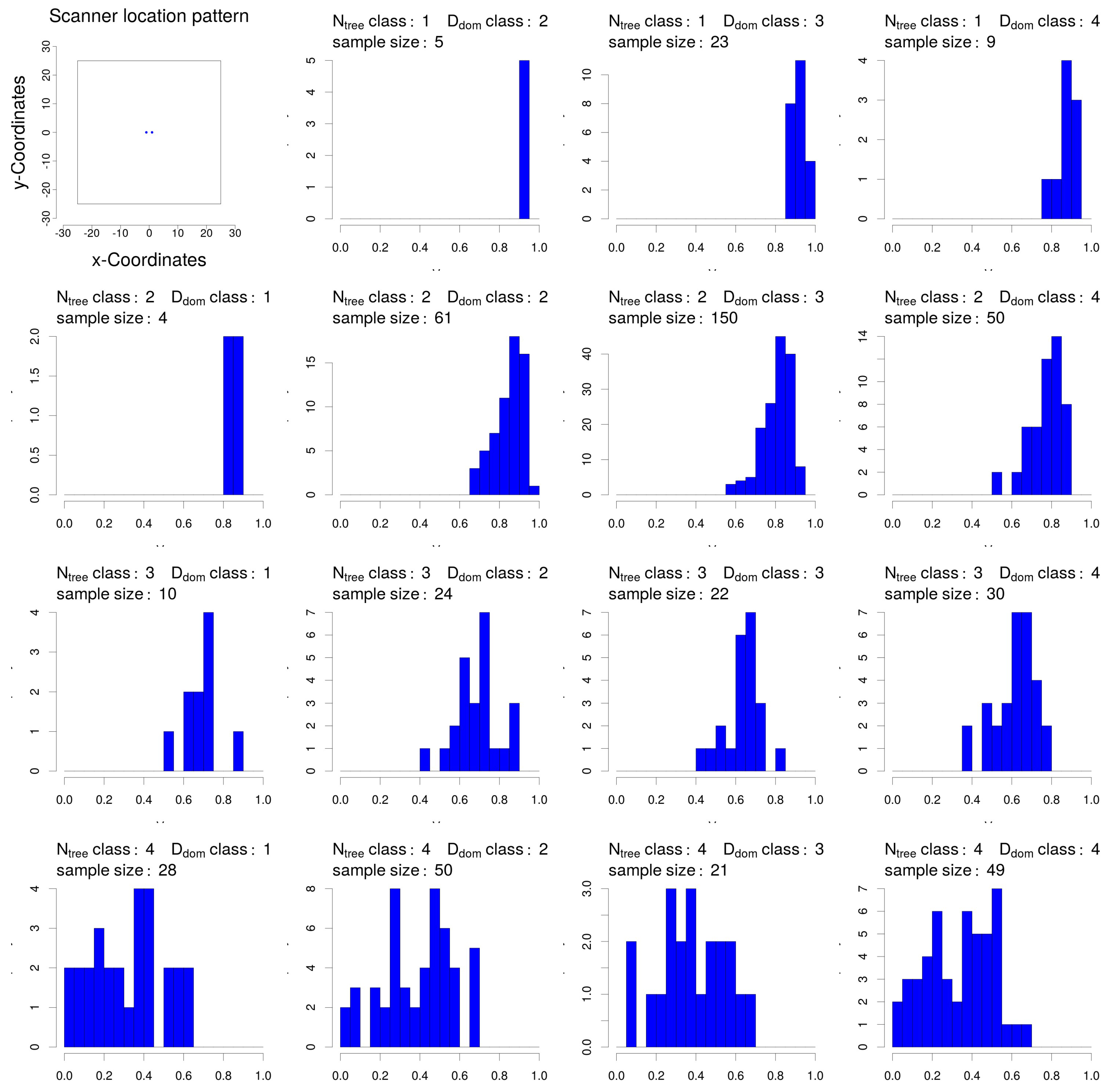
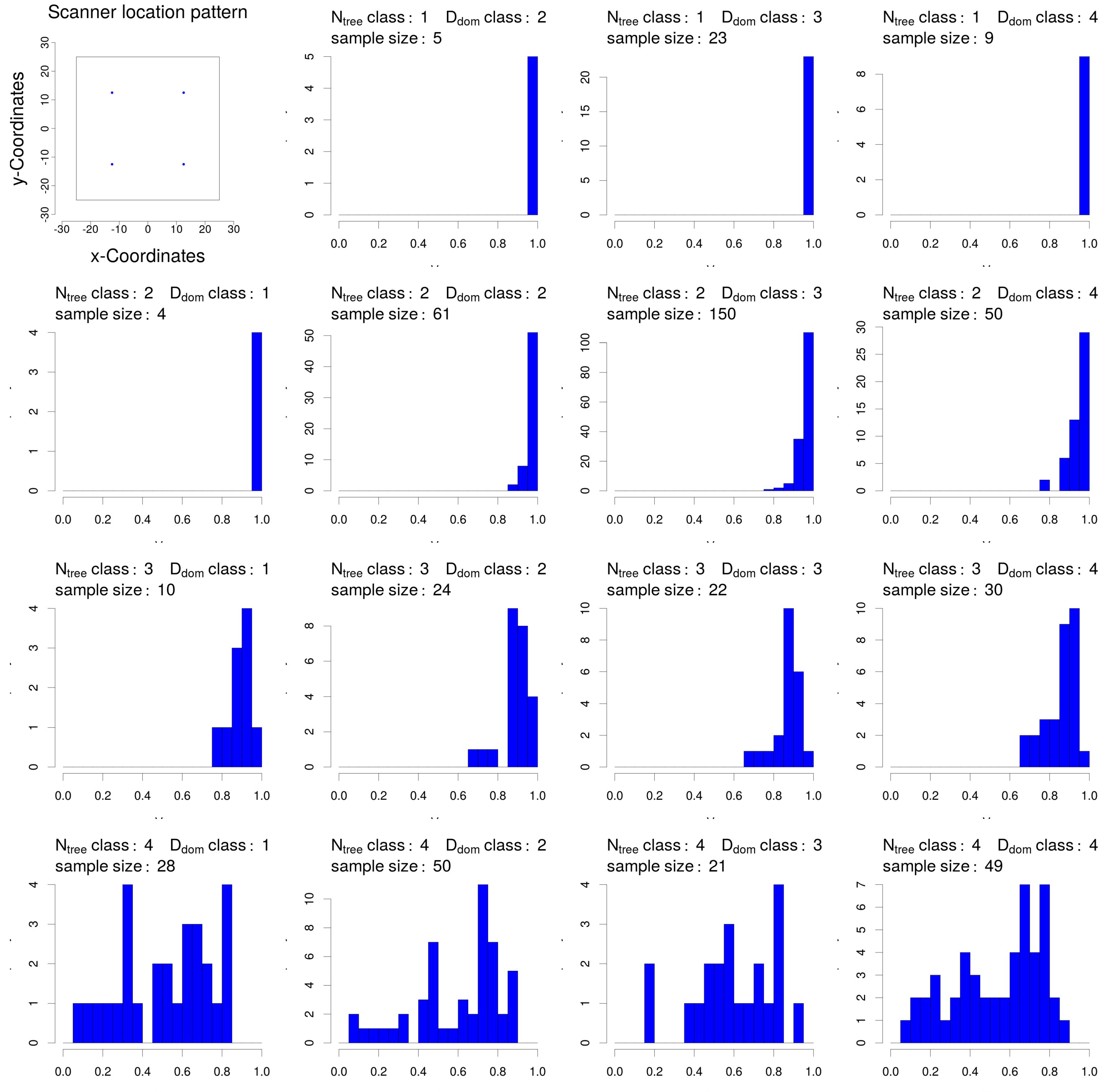
2.5. Influence of Scanner Location Patterns on Visibility in a 2D Space
3. Results
3.1. Theoretical Coverage of a Laser Scanning System in a 3D Space
3.2. Influence of Stand Parameters on Visibility in a 2D Space
3.3. Influence of the Scanning Location within Sample Plots on Visibility in a 2D Space
3.4. Influence of Scanner Location Pattern on Visibility in a 2D Space
4. Discussion
4.1. Theoretical Coverage of a Laser Scanning System in a 3D Space
4.2. Influence of Stand Parameters on Visibility in a 2D Space
4.3. Influence of the Scanning Location within Sample Plots on Visibility in a 2D Space
4.4. Influence of Scanner Location Pattern on Visibility in a 2D Space
5. Conclusions
Acknowledgments
Author Contributions
Conflicts of Interest
Abbreviations
| Horizontal distance to the centre of the sample plot | |
| DBH | Diameter at breast height |
| Diameter of the dominant (the largest) 100 trees per hectare | |
| Euclidean distance from the voxel centre to the scanner location | |
| Horizontal distance from the voxel centre to the scanner location | |
| GIS | Geographical information system |
| LiDAR | Light detection and ranging |
| NFI | National Forest Inventory |
| Number of rays (vectors) entering a voxel | |
| Number of scanning locations combined to a scanner location pattern | |
| Number of rays (vectors) that could enter a voxel without occlusion | |
| Number of trees per hectare with a minimal height of 1.3 m | |
| Number of trees per hectare with a minimal DBH of 12 cm | |
| Scanner location pattern: The pattern multiple scanning locations are combined to scan a sample plot | |
| Ratio of voxel size [m] to scanner resolution [°] | |
| TLS | Terrestrial Laser Scanning |
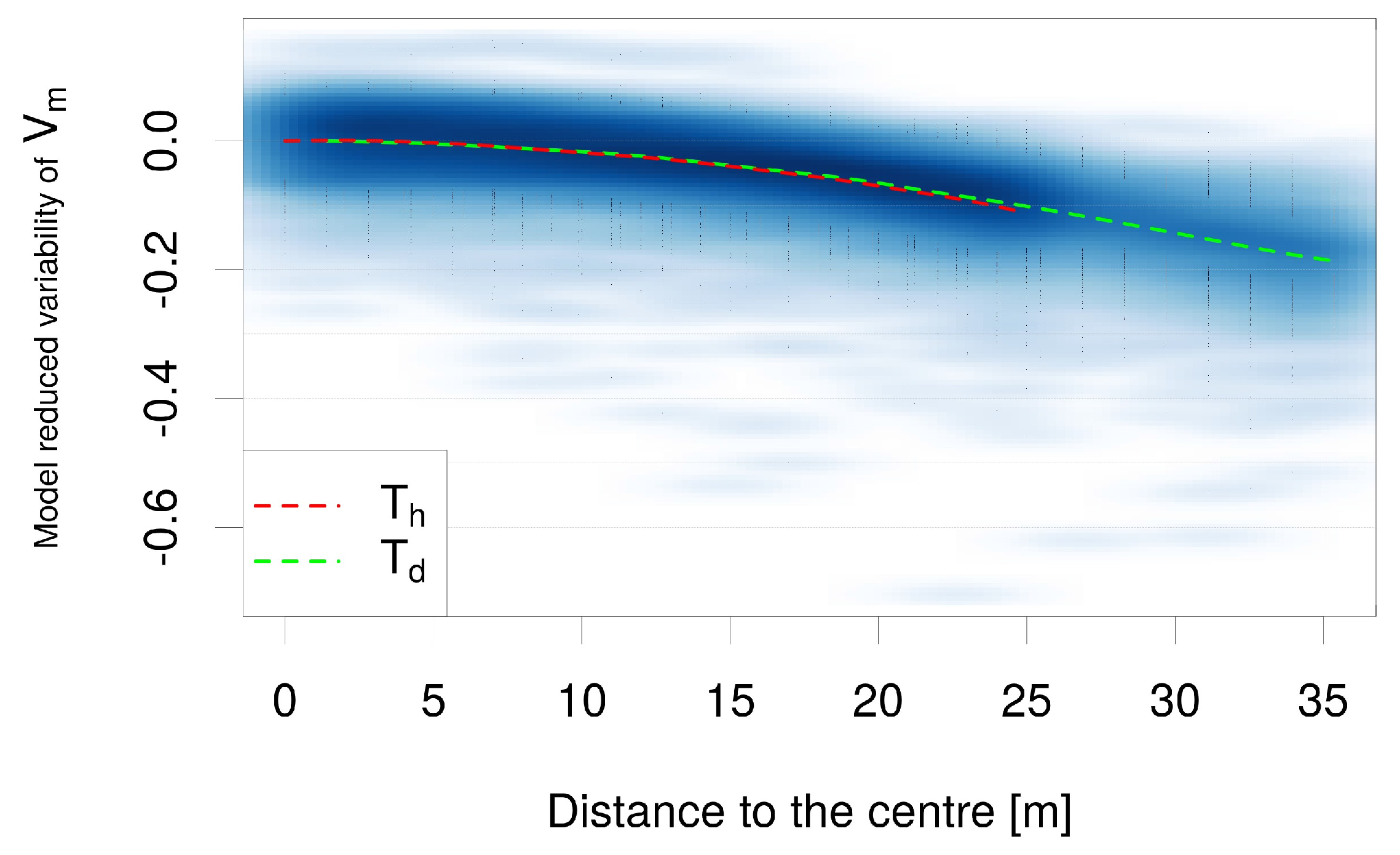
| Horizontal transect within the sample plot. The transect following the positive x axis of the local coordinate system | |
| Diagonal transect within the sample plot, ranging from the plot centre to the corner of the sample plot with coordinates (25,25) | |
| Mean visibility of the sample plot | |
| Weibull scale parameter | |
| Weibull shape parameter |
Appendix A

| -Class | ||||||
|---|---|---|---|---|---|---|
| 0–0.49 | 0.5–0.9 | 1–4.9 | 5–9.9 | 10–49.9 | >50 | |
| Distance Class | ||||||
| 0–4.9 | 14.9 | 295 | 3203 | 30,744 | 279,571 | 4,653,479 |
| 5–9.9 | 1.8 | 41 | 457 | 4453 | 38,371 | 610,737 |
| 10–14.9 | 0.5 | 15 | 174 | 1695 | 14,538 | 230,408 |
| 15–19.9 | 0.2 | 8 | 93 | 909 | 7770 | 123,584 |
| 20–24.9 | 0.1 | 4 | 58 | 575 | 4945 | 78,485 |
| 25–29.9 | 0 | 3 | 40 | 400 | 3451 | 54,917 |
| 30–49.9 | 0 | 1 | 22 | 221 | 1913 | 30,431 |
| >50 | 0 | 0 | 8 | 89 | 779 | 12,420 |

| Variable | Model Coefficient | Standardised Model Coefficient | p Value |
|---|---|---|---|
| Intercept | 2.781 | 0 | <0.0001 |
| −0.251 | −1.23 | <0.0001 | |
| −0.13 | −0.408 | <0.0001 | |
| −0.123 | −0.285 | <0.0001 | |
| 0.006 | 0.047 | <0.0001 |


References
- FOREST EUROPE. State of Europe’s Forests 2015; Ministerial Conference on the Protection of Forests in Europe: Madrid, Spain, 2015; Available online: http://enb.iisd.org/forestry/europe/mc/2015/ (accessed on 26 May 2017).
- MacDicken, K.; Jonsson, Ö.; Piña, L.; Marklund, L.; Maulo, S.; Contessa, V.; Adikari, Y.; Garzuglia, M.; Lindquist, E.; Reams, G.; et al. Global Forest Resources Assessment 2015: How Are the World’s Forests Changing? Food and Agriculture Organistation of the United Nations (FAO): Roma, Italy, 2016. [Google Scholar]
- Pan, Y.; Birdsey, R.A.; Fang, J.; Houghton, R.; Kauppi, P.E.; Kurz, W.A.; Phillips, O.L.; Shvidenko, A.; Lewis, S.L.; Canadell, J.G.; et al. A Large and Persistent Carbon Sink in the World’s Forests. Science 2011, 333, 988–993. [Google Scholar] [CrossRef] [PubMed]
- Shvidenko, A.; Barber, C.V.; Persson, R. Forest and Woodland Systems; Island Press: Washington, DC, USA, 2005; Chapter 21; pp. 585–621. [Google Scholar]
- Brassel, P.; Lischke, H. Swiss National Forest Inventory: Methods and Models of the Second Assessment; WSL Swiss Federal Research Institute: Birmensdorf, Switzerland, 2001. [Google Scholar]
- Tomppo, E.; Gschwantner, T.; Lawrence, M.; McRoberts, R.E. National Forest Inventories; Springer: Berlin, Germany, 2010. [Google Scholar]
- Lovell, J.; Jupp, D.; Newnham, G.; Coops, N.; Culvenor, D. Simulation study for finding optimal lidar acquisition parameters for forest height retrieval. For. Ecol. Manag. 2005, 214, 398–412. [Google Scholar] [CrossRef]
- Disney, M.; Lewis, P.; Raumonen, P. Testing a new vegetation structure retrieval algorithm from terrestrial lidar scanner data using 3D models. In Proceedings of the Silvilaser 2012, Vancouver, BC, Canada, 16–18 September 2012. [Google Scholar]
- Van der Zande, D.; Jonckheere, I.; Stuckens, J.; Verstraeten, W.W.; Coppin, P. Sampling design of ground-based lidar measurements of forest canopy structure and its effect on shadowing. Can. J. Remote Sens. 2008, 34, 526–538. [Google Scholar] [CrossRef]
- Binney, J.; Sukhatme, G.S. 3D tree reconstruction from laser range data. In Proceedings of the ICRA’09 IEEE International Conference on Robotics and Automation, Kobe, Japan, 12–17 May 2009. [Google Scholar]
- Watt, P.J.; Donoghue, D.N.M. Measuring forest structure with terrestrial laser scanning. Int. J. Remote Sens. 2005, 26, 1437–1446. [Google Scholar] [CrossRef]
- Trochta, J.; Kral, K.; Janik, D.; Adam, D. Arrangement of terrestrial laser scanner positions for area-wide stem mapping of natural forests. Can. J. For. Res. 2013, 43, 355–363. [Google Scholar] [CrossRef]
- Van der Zande, D.; Hoet, W.; Jonckheere, I.; van Aardt, J.; Coppin, P. Influence of measurement set-up of ground-based LiDAR for derivation of tree structure. Agric. For. Meteorol. 2006, 141, 147–160. [Google Scholar] [CrossRef]
- Hilker, T.; Coops, N.C.; Culvenor, D.S.; Newham, G.; Wulder, M.A.; Bater, C.W.; Siggins, A. A simple technique for co-registration of terrestrial LiDAR observations for forestry applications. Remote Sens. Lett. 2012, 3, 239–247. [Google Scholar] [CrossRef]
- Wezyk, P.; Koziol, K.; Glista, M.; Pierzchalski, M. Terrestrial Laser Scanning versus Traditional Forest Inventory. First Result from the Polish Forests. ISPRS Workshop on Laser Scanning 2007 and SilviLaser 2007. In Proceedings of the International Archives of the Photogrammetry, Remote Sensing and Spatial Information Sciences, Espoo, Finland, 12–14 September 2007; Volume XXXVI-3/W52, pp. 424–429. [Google Scholar]
- Yang, X.; Strahler, A.H.; Schaaf, C.B.; Jupp, D.L.B.; Yao, T.; Zhao, F.; Wang, Z.; Culvenor, D.S.; Newnham, G.J.; Lovell, J.; et al. Three-dimensional forest reconstruction and structural parameter retrievals using a terrestrial full-waveform lidar instrument (Echidna). Remote Sens. Environ. 2013, 135, 36–51. [Google Scholar] [CrossRef]
- Liang, X.; Kankare, V.; Hyyppä, J.; Wang, Y.; Kukko, A.; Haggrén, H.; Yu, X.; Kaartinen, H.; Jaakkola, A.; Guan, F.; et al. Terrestrial laser scanning in forest inventories. ISPRS J. Photogramm. Remote Sens. 2016, 115, 63–77. [Google Scholar] [CrossRef]
- Keller, M. Swiss National Forest Inventory. Manual of the Field Survey 2004–2007; Swiss Federal Research Institute WSL: Birmensdorf, Switzerland, 2011. [Google Scholar]
- Mandallaz, D. Sampling Techniques for Forest Inventories; Chapman & Hall/CRC Applied Environmental Statistics; Chapman and Hall/CRC: Boca Raton, FL, USA, 2006. [Google Scholar]
- Bailey, R.L.; Dell, T.R. Quantifying diameter distributions with the Weibull function. For. Sci. 1973, 19, 97–104. [Google Scholar]
- Blender Online Community. Blender—A 3D Modelling and Rendering Package; Blender Foundation, Blender Institute: Amsterdam, The Netherlands, 2015. [Google Scholar]
- Gschwandtner, M.; Kwitt, R.; Uhl, A.; Pre, W. BlenSor: Blender Sensor Simulation Toolbox. In Advances in Visual Computing, Proceedings of the 7th International Symposium (ISVC 2011), Las Vegas, NV, USA, 26–28 September 2011; Bebis, G., Boyle, R., Parvin, B., Koracin, D., Chung, R., Hammoud, R., Eds.; Springer: Berlin, Germany, 2011; Volume 6939/2011, pp. 199–208. [Google Scholar]
- Kükenbrink, D.; Schneider, F.D.; Leiterer, R.; Schaepman, M.E.; Morsdorf, F. Quantificationof hidden canopy volume of airborne laser scanning data using a voxel traversal algorithm. Remote Sens. Environ. 2017, 194, 424–436. [Google Scholar] [CrossRef]
- Amanatides, J.; Woo, A. A Fast Voxel Traversal Algorithm for Ray Tracing. In Proceedings of the Eurographics 87, Amsterdam, The Netherlands, 24–28 August 1987; pp. 3–10. [Google Scholar]
- Fisher, P.F. First Experiments in Viewshed Uncertainty: The Accuracy of the Viewshed Area. Photogramm. Eng. Remote Sens. 1991, 57, 1321–1327. [Google Scholar]
- Travis, M.R.; Elsner, G.H.; Iverson, W.D.; Johnson, C.G. VIEWIT: Computation of Seen Areas, Slope, and Aspect for Land-Use Planning; Technical Report; Pacific Southwest Research Station; Forest Service; U.S. Department of Agriculture: Berkeley, CA, USA, 1975.
- Gaulton, R.; Danson, F.; Ramirez, F.; Gunawan, O. The potential of dual-wavelength laser scanning for estimating vegetation moisture content. Remote Sens. Environ. 2013, 132, 32–39. [Google Scholar] [CrossRef]
- R Core Team. R: A Language and Environment for Statistical Computing; R Foundation for Statistical Computing: Vienna, Austria, 2017. [Google Scholar]
- Mosteller, F.; Tukey, J.W. Data Analysis and Regression: A Second Course in Statistics; Addison-Wesley: Boston, MA, USA, 1977. [Google Scholar]
- Antonarakis, A.S. Evaluating forest biometrics obtained from ground lidar in complex riparian forests. Remote Sens. Lett. 2011, 2, 61–70. [Google Scholar] [CrossRef]
- Liang, X.; Hyyppä, J. Automatic Stem Mapping by Merging Several Terrestrial Laser Scans at the Feature and Decision Levels. Sensors 2013, 13, 1614–1634. [Google Scholar] [CrossRef] [PubMed]
- Liang, X.; Kankare, V.; Yu, X.; Hyyppä, J.; Holopainen, M. Automated Stem Curve Measurement Using Terrestrial Laser Scanning. IEEE Trans. Geosci. Remote Sens. 2014, 52, 1739–1748. [Google Scholar] [CrossRef]
- Thies, M.; Pfeifer, N.; Winterhalder, D.; Gorte, B. Three-dimensional reconstruction of stems for assessment of taper, sweep and lean based on laser scanning of standing trees. Scand. J. For. Res. 2006, 19, 571–581. [Google Scholar] [CrossRef]
- Bienert, A.; Scheller, S.; Keane, E.; Mullooly, G.; Mohan, F. Application of terrestrial laser scanners for the determination of forest inventory parameters. Commission V Symposium ’Image Engineering and Vision Metrology’. In Proceedings of the International Archives of the Photogrammetry, Remote Sensing and Spatial Information Sciences, Dresden, Germany, 25–27 September 2006; Volume XXXVI, part 5. p. 5. [Google Scholar]
- Maas, H.G.; Bienert, A.; Scheller, S.; Keane, E. Automatic forest inventory parameter determination from terrestrial laser scanner data. Int. J. Remote Sens. 2008, 29, 1579–1593. [Google Scholar] [CrossRef]
- Côté, J.F.; Fournier, R.A.; Frazer, G.W.; Niemann, K.O. A fine-scale architectural model of trees to enhance LiDAR-derived measurements of forest canopy structure. Agric. For. Meteorol. 2012, 166–167, 72–85. [Google Scholar] [CrossRef]
- Simonse, M.; Aschoff, T.; Spiecker, H.; Thies, M. Automatic Determination of Forest Inventory Parameters using Terrestrial Laser Scanning. In Proceedings of the ScandLaser Scientific Workshop on Airborne Laser Scanning of Forests, Umeå, Sweden, 3–4 September 2003; pp. 251–257. [Google Scholar]
- Eysn, L.; Pfeifer, N.; Ressl, C.; Hollaus, M.; Grafl, A.; Morsdorf, F. A Practical Approach for Extracting Tree Models in Forest Environments Based on Equirectangular Projections of Terrestrial Laser Scans. Remote Sens. 2013, 5, 5424–5448. [Google Scholar] [CrossRef]
- Yao, T.; Yang, X.; Zhao, F.; Wang, Z.; Zhang, Q.; Jupp, D.; Lovell, J.; Culvenor, D.; Newnham, G.; Ni-Meister, W.; et al. Measuring forest structure and biomass in New England forest stands using Echidna ground-based lidar. Remote Sens. Environ. 2011, 115, 2965–2974. [Google Scholar] [CrossRef]
- Calders, K.; Newnham, G.; Burt, A.; Murphy, S.; Raumonen, P.; Herold, M.; Culvenor, D.; Avitabile, V.; Disney, M.; Armston, J.; et al. Nondestructive estimates of above-ground biomass using terrestrial laser scanning. Methods Ecol. Evol. 2015, 6, 198–208. [Google Scholar] [CrossRef]
- Woodgate, W.; Armston, J.D.; Disney, M.; Jones, S.D.; Suarez, L.; Hill, M.J.; Wilkes, P.; Soto-Berelov, M. Quantifying the impact of woody material on leaf area index estimation from hemispherical photography using 3D canopy simulations. Agric. For. Meteorol. 2016, 226–227, 1–12. [Google Scholar] [CrossRef]
- Newnham, G.J.; Armston, J.D.; Calders, K.; Disney, M.I.; Lovell, J.L.; Schaaf, C.B.; Strahler, A.H.; Danson, F.M. Terrestrial Laser Scanning for Plot-Scale Forest Measurement. Curr. For. Rep. 2015, 1, 239–251. [Google Scholar] [CrossRef]
- Dassot, M.; Constant, T.; Fournier, M. The use of terrestrial LiDAR technology in forest science: Application fields, benefits and challenges. Ann. For. Sci. 2011, 68, 959–974. [Google Scholar] [CrossRef]
- Raumonen, P.; Kaasalainen, M.; Akerblom, M.; Kaasalainen, S.; Kaartinen, H.; Vastaranta, M.; Holopainen, M.; Disney, M.; Lewis, P. Fast automatic Precision Tree Models from Terrestrial Laser Scanner Data. Remote Sens. 2013, 5, 491–520. [Google Scholar] [CrossRef]
- Hackenberg, J.; Morhart, C.; Sheppard, J.; Spiecker, H.; Disney, M. Highly Accurate Tree Models Derived from Terrestrial Laser Scan Data: A Method Description. Forests 2014, 5, 1069–1105. [Google Scholar] [CrossRef]
- Stoyan, D.; Stoyan, H. Non-Homogeneous Gibbs Process Models for Forestry—A Case Study. Biom. J. 1998, 40, 521–531. [Google Scholar] [CrossRef]
- Law, R.; Illian, J.; Burslem, D.F.R.P.; Gratzer, G.; Gunatilleke, C.V.S.; Gunatilleke, I.A.U.N. Ecological information from spatial patterns of plants: Insights from point process theory. J. Ecol. 2009, 97, 616–628. [Google Scholar] [CrossRef]
- Penttinen, A.; Stoyan, D.; Henttonen, H.M. Marked Point PrProcess in Forest Statistics. For. Sci. 1992, 38, 806–824. [Google Scholar]
- Hopkinson, C.; Chasmer, L.; Young-Pow, C.; Treitz, P. Assessing forest metrics with a ground-based scanning lidar. Can. J. For. Res. 2004, 34, 573–583. [Google Scholar] [CrossRef]
- Kelbe, D.; Romanczyk, P.; van Aardt, J.; Cawse-Nicholson, K.; Krause, K. Automatic extraction of tree stem models from single rerrestrial lidar scans in structurally heterogeneous forest environments. In Proceedings of the Silvilaser 2012, Vancouver, BC, Canada, 16–18 September 2012. [Google Scholar]
- Abegg, M.; Brändli, U.B.; Cioldi, F.; Fischer, C.; Herold-Bonardi, A.; Huber, M.; Keller, M.; Meile, R.; Rösler, E.; Speich, S.; et al. Viertes Schweizerisches Landesforstinventar–Ergebnistabellen und Karten im Internet zum LFI 2009–2013 (LFI4b). 2014. Available online: https://doi.org/10.21258/1000001 (accessed on 25 May 2017).


| Variable | Model Coefficient | Standardised Model Coefficient | p Value |
|---|---|---|---|
| Intercept | 8.38 | 0 | <0.0001 |
| log () | −0.9 | −0.22 | <0.0001 |
| log () | −1.09 | −0.18 | <0.0001 |
| log () | 2.03 | 0.92 | <0.0001 |
| Variable | Model Coefficient | Standardised Model Coefficient | p Value |
|---|---|---|---|
| Intercept | 2.726 | 0 | <0.0001 |
| −0.249 | −1.211 | <0.0001 | |
| −0.124 | −0.384 | <0.0001 | |
| −0.116 | −0.271 | <0.0001 | |
| 0.008 | 0.06 | <0.0001 |
| Scanner Location Pattern | Combined Locations | Mean | Standard Deviation of |
|---|---|---|---|
| 0 | 32, 34 | 0.67 | 0.23 |
| 1 | 63, 61 | 0.69 | 0.24 |
| 2 | 42, 44 | 0.69 | 0.24 |
| 3 | 22, 24 | 0.65 | 0.25 |
| 4 | 51, 53 | 0.68 | 0.24 |
| 5 | 11, 13 | 0.52 | 0.26 |
| 6 | 11, 51 | 0.57 | 0.24 |
| 7 | 11, 0 | 0.63 | 0.25 |
| 8 | 11, 53 | 0.61 | 0.25 |
| 9 | 42, 32 | 0.68 | 0.24 |
| 10 | 42, 0 | 0.69 | 0.24 |
| 11 | 42, 34 | 0.69 | 0.24 |
| 12 | 0, 34, 32 | 0.72 | 0.22 |
| 13 | 0, 61, 63 | 0.78 | 0.23 |
| 14 | 0, 51, 53 | 0.78 | 0.23 |
| 15 | 0, 11, 13 | 0.71 | 0.26 |
| 16 | 53, 43, 52 | 0.75 | 0.23 |
| 17 | 53, 33, 52 | 0.77 | 0.23 |
| 18 | 53, 0, 52 | 0.77 | 0.23 |
| 19 | 53, 31, 52 | 0.77 | 0.23 |
| 20 | 53, 41, 52 | 0.78 | 0.23 |
| 21 | 31, 32, 33, 34 | 0.76 | 0.21 |
| 22 | 61, 62, 63, 64 | 0.84 | 0.21 |
| 23 | 41, 42, 43, 44 | 0.84 | 0.21 |
| 24 | 51, 52, 53, 54 | 0.84 | 0.21 |
| 25 | 11, 12, 13, 14 | 0.71 | 0.28 |
| 26 | 51, 62, 53, 64 | 0.84 | 0.21 |
| 27 | 51, 61, 53, 63 | 0.83 | 0.22 |
| 28 | 33, 43, 52, 62 | 0.81 | 0.22 |
| 29 | 11, 12, 13, 0 | 0.76 | 0.26 |
| 30 | 0, 31, 32, 33, 34 | 0.78 | 0.21 |
| 31 | 0, 41, 42, 43, 44 | 0.86 | 0.2 |
| 32 | 0, 51, 52, 53, 54 | 0.87 | 0.19 |
| 33 | 62, 51, 52, 53, 54 | 0.87 | 0.2 |
| 34 | 42, 51, 52, 53, 54 | 0.87 | 0.2 |
| 35 | 32, 51, 52, 53, 54 | 0.87 | 0.19 |
| 36 | 0, 41, 61, 62, 43, 63, 64 | 0.9 | 0.17 |
| 37 | 53, 43, 52, 44, 0, 42, 54, 41, 51 | 0.92 | 0.15 |
| 38 | 53, 43, 52, 44, 0, 42, 54, 41, 11 | 0.92 | 0.16 |
| 39 | 53, 43, 52, 44, 0, 42, 54, 41, 61 | 0.92 | 0.15 |
© 2017 by the authors. Licensee MDPI, Basel, Switzerland. This article is an open access article distributed under the terms and conditions of the Creative Commons Attribution (CC BY) license (http://creativecommons.org/licenses/by/4.0/).
Share and Cite
Abegg, M.; Kükenbrink, D.; Zell, J.; Schaepman, M.E.; Morsdorf, F. Terrestrial Laser Scanning for Forest Inventories—Tree Diameter Distribution and Scanner Location Impact on Occlusion. Forests 2017, 8, 184. https://doi.org/10.3390/f8060184
Abegg M, Kükenbrink D, Zell J, Schaepman ME, Morsdorf F. Terrestrial Laser Scanning for Forest Inventories—Tree Diameter Distribution and Scanner Location Impact on Occlusion. Forests. 2017; 8(6):184. https://doi.org/10.3390/f8060184
Chicago/Turabian StyleAbegg, Meinrad, Daniel Kükenbrink, Jürgen Zell, Michael E. Schaepman, and Felix Morsdorf. 2017. "Terrestrial Laser Scanning for Forest Inventories—Tree Diameter Distribution and Scanner Location Impact on Occlusion" Forests 8, no. 6: 184. https://doi.org/10.3390/f8060184