Tree Density and Forest Productivity in a Heterogeneous Alpine Environment: Insights from Airborne Laser Scanning and Imaging Spectroscopy

Abstract

We outline an approach combining airborne laser scanning (ALS) and imaging spectroscopy (IS) to quantify and assess patterns of tree density (TD) and forest productivity (FP) in a protected heterogeneous alpine forest in the Swiss National Park (SNP). We use ALS data and a local maxima (LM) approach to predict TD, as well as IS data (Airborne Prism Experiment—APEX) and an empirical model to estimate FP. We investigate the dependency of TD and FP on site related factors, in particular on surface exposition and elevation. Based on reference data (i.e., 1598 trees measured in 35 field plots), we observed an underestimation of ALS-based TD estimates of 40%. Our results suggest a limited sensitivity of the ALS approach to small trees as well as a dependency of TD estimates on canopy heterogeneity, structure, and species composition. We found a weak to moderate relationship between surface elevation and TD (R² = 0.18–0.69) and a less pronounced trend with FP (R² = 0.0–0.56), suggesting that both variables depend on gradients of resource availability. Further to the limitations faced in the sensitivity of the applied approaches, we conclude that the combined application of ALS and IS data was convenient for estimating tree density and mapping FP in north-facing forested areas, however, the accuracy was lower in south-facing forested areas covered with multi-stemmed trees.

1. Introduction

Tree density (TD) and forest productivity (FP) are important structural and functional variables of forest ecosystems. TD, defined as the number of trees per unit area [1], along with other structural information (e.g., species composition, canopy closure, tree height, and timber volume), is fundamental for forest management planning [2]. TD provides, indirectly, information on stand basal area, timber volume [3], and aboveground carbon storage [4]. In managed forest ecosystems, TD information allows forest managers to indicate essential treatments such as thinning, or to develop strategies to increase regeneration rates if the number of trees is too small [5]. Particularly in unmanaged and protected forests, TD is crucial to determine forest succession dynamics [6], and to assess spatio-temporal patterns in tree mortality [7]. Gross primary production (GPP), defined as the capacity of a forest to gain carbon through photosynthesis over a given time period, has been widely used to quantify FP [8,9]. FP is important to understand feedbacks of forests to climate change (i.e., rising atmospheric CO₂ concentrations [10]) and other natural disturbances such as insect and pathogen attacks [11]. Further, FP information facilitates the design of optimal silvicultural guidelines [12], and multi-temporal assessments of FP have shown a great potential to assess growth patterns of different forest types including virgin, natural or managed forests [13].

TD and FP balance each other since both are determined by the availability of resources, are complementary information variables to characterize forest ecosystems, and are valuable input for broad-scale modeling of biological and biogeochemical processes [14]. Understanding the relationship between FP and TD is important for ecologists and forest managers [15]. However, few studies have exploited inter-dependencies at larger ecosystem scales so far [16]. Further, ecologists are interested in abiotic components such as topography that often has a strong influence on structure, composition, and function of forest ecosystems [17]. Topography (i.e., elevation) has been identified as an easy proxy for resource availability and spatial patterns of ecosystem properties [18]. Changes in elevation, particularly across large gradients, can introduce major changes in community-averaged leaf traits [19], which in turn may affect FP. Asner et al. [20] emphasized the lack of knowledge about the contribution of elevation on plant functional traits at different scales. Such information would allow modeling and prediction of spatial variation in ecosystem processes at any given point along elevation gradients. In addition, the interrelation between FP and TD with elevation can also provide crucial information to determine tree-line elevation [21]. Nevertheless, the assessment of such relations between forest functional and structural attributes remains largely underrepresented at ecosystem scale.

Field surveys are still the most accurate approach to collect structural forest attributes [22,23]. The advantage of the high accuracy achievable is often counterbalanced by substantial costs and difficulties in obtaining information for large, remote, and structurally complex forest areas [3]. Further, providing continuous information of forest attributes typically requires additional interpolation approaches that are prone to error [23]. With the launch of the first Earth observation (EO) satellites in the 1970s, substantial efforts have been conducted to find alternatives to traditional field surveys. Nowadays, the use of EO data and information extraction approaches are an important alternative to complement mapping of forest attributes, particularly for large areas [24,25,26].

Estimates of TD from both active and passive EO systems have been widely performed [25,26,27,28,29]. In particular, airborne laser scanning (ALS) holds a large potential to accurately measure the three-dimensional distribution of forest structural components [30,31,32], and has become an essential component for operationalizing forest inventories in various countries [33,34]. Estimates of TD from ALS data can be obtained either from area-based approaches (ABAs) or from individual tree detection approaches (ITD) [35]. ABAs are often based on empirical relationships between measured TD at plot or stand level and corresponding ALS-derived metrics (e.g., canopy height, height percentiles, canopy closure, and crown diameter) [36,37]. Although ABAs are commonly applied in operational forestry applications [38], they show several limitations (i.e., they are dependent on extensive in situ data [36,37], they are site-specific [39], and they are limited in sensitivity to TD [40]). In contrast, ITD-based approaches utilize either ALS point cloud data or canopy height models (CHM) to identify individual trees [35,38,41]. Plot or stand estimates are obtained afterwards by summing up identified trees. Kaartinen et al. [42] indicate that ITD approaches provide true stem distribution series and require less in situ data compared to ABAs. ITD approaches are, however, currently under development and have not yet been widely applied in practice, or across heterogeneous forests in terms of structural complexity, species composition, and silvicultural treatments [38,42].

FP can be approximated with GPP, which itself can stem from various approaches ranging from empirical to process-based modeling approaches. Empirical approaches based on optical EO data are simple to implement, but rely on extensive in situ data and are thus site- and ecosystem-specific. A frequently-used approach to mapping FP exploits optical EO data in combination with Monteith’s light use efficiency model [21,43,44]. Both terms in Monteith’s equation, i.e., absorbed photosynthetic active radiation (APAR) and light use efficiency (LUE), are typically parameterized with greenness-based indices and semi-empirical modeling. Assumptions inherent to this approach (i.e., approximation of potential rather than actual photosynthesis), however, limit the representativeness of obtained GPP values [45] across ecosystems (cf. Turner et al. [46] for an assessment of the MODIS-GPP product (MOD17), or Coops et al. [47] for an evaluation of other satellite-based approaches). A recent achievement in optical remote sensing is the measurement of sun-induced chlorophyll fluorescence (SIF). SIF is the most direct measurement of plant photosynthesis, and opens new perspectives on constraining estimates of GPP across ecosystems [48,49]. Although this new EO approach is already well matured, certain components (e.g., the integration of SIF in photosynthesis models) remain to be fully developed in order to operationally apply SIF measurements. The use of process-based models provides the most mechanistic approach, but requires precise and detailed information on soil, climate, and additional forest properties that are often lacking or are inaccurate [44].

The above argumentation yields two research needs that are addressed in this study. This includes (i) the evaluation of pragmatic and less data driven ALS and imaging spectroscopy (IS)-based approaches for obtaining reliable estimates of TD and FP in heterogeneous forest environments, and (ii) the advancement of knowledge about the mechanistic interrelation of TD and FP with surface elevation. In particular, we estimate TD in a heterogeneous mountain forest using a combination of an ITD approach and ALS data, and validate results with in situ data. Further, we estimate FP using an empirical greenness-based approach in combination with data of the Airborne Prism Experiment (APEX) imaging spectrometer. Last, we investigate the relationship between TD and FP and evaluate the impact of topography (i.e., surface exposition and elevation) on these two important forest variables.

2. Materials and Methods

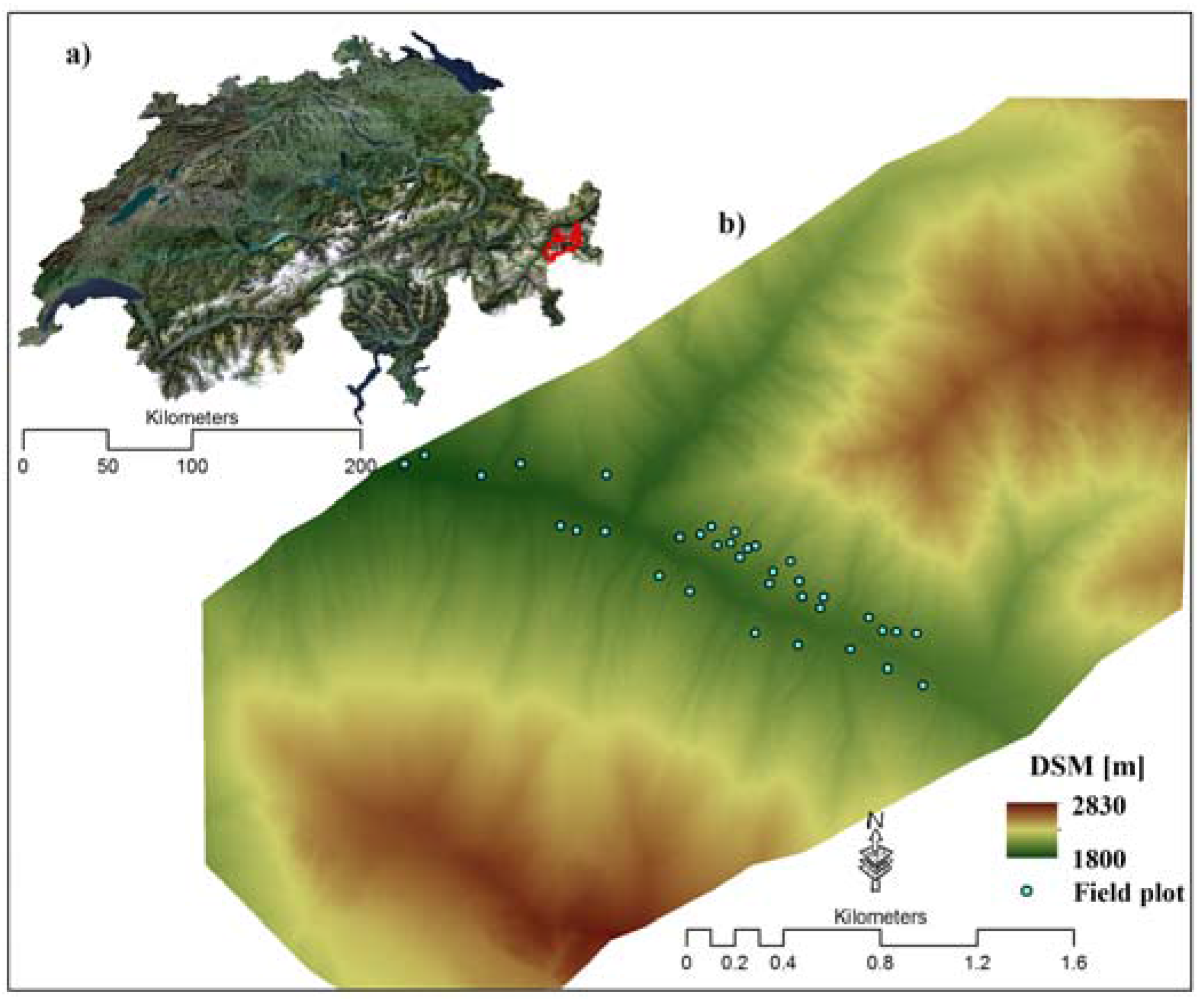
2.1. Study Area

The study area Trupchun valley (Val Trupchun) extends over a 22 km² area within the Swiss National Park (SNP), located in the southeast of Switzerland (Figure 1) The region is a heterogeneous alpine landscape with a dry and harsh climate. The mean annual precipitation totals 744 mm and the average annual temperature is 0.9 °C [50]. The study area is characterized by rough topography and steep slopes [51] with an elevation range from 1800 to 2830 m above sea level (a.s.l.) [52]. The forest is classified as boreal-type forest, dominated by European larch (Larix decidua L.), with a changing proportion of Norway spruce (Picea abies (L.) Karst) and Swiss stone pine (Pinus cembra L.) (associated species). Norway spruce trees dominate at lower altitudes, whereas Swiss stone pines are present in the high altitudes [2]. The trees are up to 250 years old and the forest ecosystem has been protected since 1914 [53].

2.2. Field Data

A stratified random sampling approach was established in June and July 2012 to collect ground information describing the forest ecosystem (Figure 1). A total of 35 squared field plots with a size of 30 m × 30 m were inventoried. During the field data collection, a slope correction factor depending on the slope angle was applied to convert the plot size into its equivalent on a horizontal plane [54]. The slope angle was measured by a SUUNTO clinometer device (Suunto, Vantaa, Finland) [55]. The identified plots represent most of the present tree species and their properties, i.e., canopy cover, density, and species composition. The geographical position of each field plot was recorded using a differential global positioning system (DGPS) with an accuracy of ±30 cm (Trimble Geo XH, Sunnyvale, CA, USA). In each plot, all trees having a diameter at breast height (DBH) larger than 5 cm were counted, corresponding DBHs and species types were recorded as well [3]. The selection of the 5 cm DBH threshold is justified by common practice in forest inventory [56]. TD was calculated as the number of trees per hectare by summing up all measured trees in each field plot [5].

In total, 1598 trees were counted in all plots, while European larches compose 718 trees (45%), Swiss stone pine 602 trees (38%), and Norway spruce 278 trees (17%). Considering the basal area per plot, European larches account for 59% of the total, followed by Swiss stone pines (29%), and Norway spruce trees (12%). Descriptive statistics of TD obtained from all field plots for the Val Trupchun area can be found in

Table 1. Tree density (TD) statistics for field plots in Val Trupchun.

Parameter	DBH > 5 cm	DBH > 12 cm	DBH > 20 cm	DBH > 30 cm	South-Facing	North-Facing
Number of plots [-]	35	35	35	35	25	10
Number of trees [-]	1598	1360	1103	691	1314	284
Tree density [N/ha]
Mean	507	432	350	219	584	316
Minimum	122	122	89	56	122	122
Maximum	1067	755	600	456	1067	644
Standard deviation	249	189	141	96	238	161

DBH: diameter at breast height.

. The mean TD amounts to up to 507 trees per ha. This is in line with findings by Risch et al. [57] who reported a value of 473 ± 90 trees per ha for this study area. We implemented various DBH thresholds to calculate the corresponding number of trees per ha. Due to different environmental factors for north-facing and south-facing slopes (i.e., solar radiation, water and soil nutrient availability) [12], we classified our field plots into north- and south-facing plots.

Table 1 shows large differences of TD’s for south- and north-facing field plots. Results of an independent sample t-test [58] prove that this difference is statistically significant (t(33) = 3.269, p = 0.003). The reasons for these differences are primarily environmental factors, natural disturbances, and historical human activity before 1914 (i.e., charcoal production, timber harvesting) [53,57,59]; multiple-stemmed trees frequently exist on south-facing areas, while high self-thinning due to light competition among trees causes the smaller TD on north-facing areas.

2.3. Airborne Imaging Spectroscopy Data

APEX is an airborne imaging spectrometer measuring radiation in the spectral range between 350 nm and 2500 nm in 284 contiguous spectral bands [60]. It was operated at an altitude of 6500 m a.s.l. over the study area on 12 July 2013, around 11:30 a.m. local time. The solar zenith angle and the solar azimuth angle were 28.1° and 139.1°, respectively. Surface height differences and slope changes cause a varying ground sampling distance across the flight line (i.e., between 1.5–3.0 m), and data were resampled to a 2 m pixel grid.

APEX data were geometrically corrected using a parametric geocoding approach (PARGE) [61]. Based on 15 ground control points that represent topographic diversity, a root mean square error (RMSE) of 3.2 m ± 1.4 m was calculated. Considering the final aggregated pixel size of 30 m × 30 m in our analysis, the achieved geometrical accuracy is acceptable. The atmospheric correction software (ATCOR-4) was used to compensate for atmospheric effects, to minimize illumination changes due to topography, and to eventually retrieve top-of-canopy hemispherical conical reflectance factor (HCRF) data [62] (for terminology see [63]). ATCOR-4 uses look-up-tables (LUT) of atmospheric functions (i.e., up- and down-welling transmittances, path scattered radiance, spherical albedo), pre-calculated with the atmospheric radiative transfer code MODTRAN-5 [64]. We assumed a mid-latitude summer atmosphere type and a rural aerosol model and estimated water vapor as well as aerosol load pixel-wise to select LUT entries for subsequent compensation of atmospheric absorption and scattering effects. We further applied the ATCOR-4 supported correction of topography induced illumination changes using a coarse resolution (i.e., 25 m spatial resolution) digital elevation model.

2.4. Airborne Laser Scanning Data

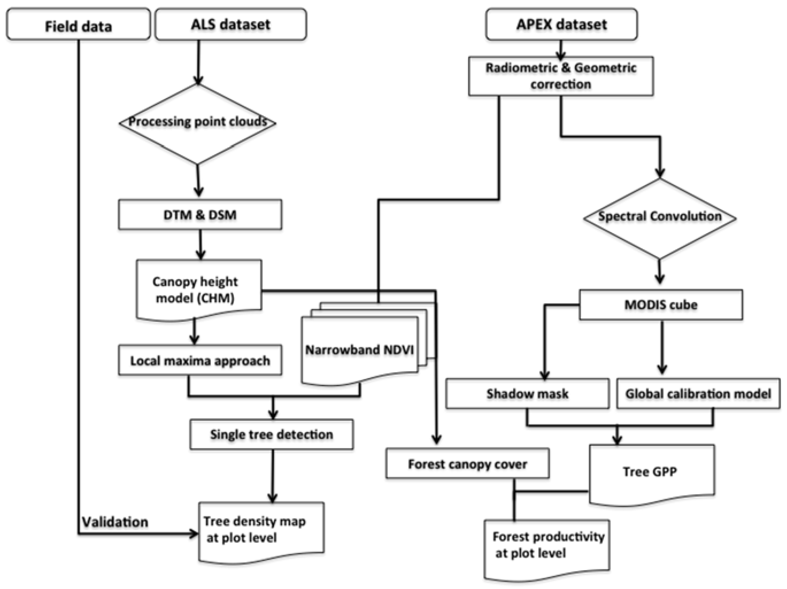
ALS data were acquired by Vermessung AVT ZT-GmbH, Imst, Austria (http://www.avt.at/home.html) in August 2011 using a double-scanner setup (LMS-Q560, RIEGL Laser Measurements Systems GmbH, Horn, Austria) mounted on a helicopter. Details of the sensor are discussed in Wagner et al. [65] and given in the technical sensor documentation provided by RIEGL [66]. Multiple returns were recorded for each emitted pulse and converted into a three-dimensional point cloud composed of planimetric coordinates (x and y) and ellipsoidal heights (z) [67]. The data cover an area of approximately 140 km² with an average point density of >5 pts/m². The point cloud was classified into ground, vegetation, water, and buildings using the TerraScan software (http://www.terrasolid.com/products/terrascanpage.php). Based on this classification, a digital terrain model (DTM) and a digital surface model (DSM) with a spatial resolution of 1 × 1 m were processed using SCOP++ (http://photo.geo.tuwien.ac.at/software/scop/). The canopy height model (CHM) with a spatial resolution of 1 × 1 m was subsequently calculated by subtracting the DTM from the DSM (cf. Hollaus et al. [68]). According to Jakubowski et al. [69], the pulse densities are high enough to enable accurate estimates of the actual canopy heights. A forest map was derived afterwards by applying a threshold to the CHM. The minimum tree height threshold was set to 3 m as utilized in the Swiss National Forest Inventory [70].

3. Methods

3.1. Local Maxima Approach to Estimate Tree Density Using ALS Data

The initial step for estimating TD using an ITD approach is the detection of individual trees. For this purpose, we used a CHM [41] that was smoothed with a Gaussian smoothing (function value of 0.7) to remove small variations in the canopy surface [71]. The Gaussian of 0.7 was chosen as most of the trees in the study area form canopies with, in contrast to CHMs in mixed or deciduous forests, typical uniform patterns in the CHM [24]. The local maxima (LM) approach is the most widely used approach for CHM-based tree detection [33] among various methods available (e.g., valley-following [72], multiple scale edge [73], watershed segmentation [74], and local maxima finding [75,76]). The relatively simple LM approach is fast and easy to implement [3,42], and identifies the top of a tree crown as the pixel containing the highest value above ground compared to all pixels in a specific neighborhood [24,75]. Considering different canopy dimensions/canopy widths, we applied the LM-approach with variable spatial resolutions of the CHM (i.e., 1 m × 1 m and 2 m × 2 m grid-cell resolution) and a moving window size of 3 × 3 pixels. On very steep slopes, ALS echoes from the tree understory (e.g., grass, ground) can have an altitudinal range larger than 3 m within the target grid-cell size of 1 m, causing uncertain CHM values of >3 m. We applied a narrow-band NDVI (Normalized Differenced Vegetation Index) product obtained from APEX data (spectral bands at 665 and 831 nm) to remove such falsely detected trees in complex terrain (cf. Khosravipour et al. [77]) The identified treetops were summed up afterwards to calculate the TD per plot.

3.2. Spatial Modeling of Forest Productivity Using APEX Data

FP was approximated with forest GPP as suggested in [78]. GPP was obtained using a simple global calibration equation as introduced by Hashimoto et al. [79] that relates GPP to the Enhanced Vegetation Index (EVI). The EVI was calculated according to Huete et al. [80] as:

$$\mathrm{EVI}=\mathrm{G}\frac{{\rho }_{NIR-}{\rho }_{red}}{{\rho }_{NIR}+ C_1\times {\rho }_{red} - C_{2 }\times {\rho }_{blue }+L}$$

(1)

where ρ indicates the surface HCRF for the near infrared (NIR), red and blue band, and L (1) is a canopy background adjustment. G (2.5) is the gain factor and C₁ (6) and C₂ (7.5) are band-specific atmospheric resistance correction coefficients. All values and the coefficients have been optimized for the MODIS EVI product [80]. We therefore spectrally convolved APEX HCRF data to match the spectral resolution of respective MODIS bands and assumed validity of both gain factors (i.e., C₁ and C₂) for the higher spatial resolution of our data as demonstrated in [81,82,83]. However, the differences in spatial resolution (i.e., 2 m of APEX vs. 500 m of MODIS) require further consideration. The high spatial resolution of APEX yields detailed measurements of forest ecosystems, including shaded and illuminated parts of tree crowns. These illumination patterns are primarily caused by geometric optical scattering and complicate the description of radiative transfer, particularly in shaded canopy areas, eventually impacting the accuracy of retrieved vegetation indices [84] and estimated GPP. Geometric-optical scattering scales with spatial resolution and its impact decreases with increasing ground-sampling distances. We consequently masked shaded pixels using an empirical threshold approach to be in better correspondence with the differently resolved MODIS and APEX measurements. FP, the carbon uptake by all trees of a specific forested area, was eventually obtained by averaging resulting GPP values of tree crowns for a 30 m grid cell and normalizing for tree fractional cover in the respective area. Fractional cover of the 30 m grid cell was estimated from the ALS based CHM (Figure 2).

We are aware of the limitations in using EVI to estimate GPP, since it is representative for potential, rather than actual, photosynthetic activity only. However, the study area is highly complex in terms of topography and we lack reliable data to facilitate new approaches (i.e., SIF-based GPP estimates [49]). We consequently applied the greenness-based approach using the EVI to obtain first limited insights into GPP distribution in alpine environments.

3.3. Validation

The accuracy of ALS-based TD estimates was assessed using field measurements at plot level. The validation procedure was applied to all field plots, and individually to those located on south-facing and north-facing slopes. The agreement was assessed by calculating the coefficient of determination (R²), the root mean square error (RMSE), and the relative RMSE (RMSE%). A quantitative validation of FP was not possible, due to the lack of adequate data. Instead, we used in situ measurements of annual GPP of a close-by forest ecosystem similar to the one of our study site and assumed consistency of the algorithm performance across these two test sites.

4. Results

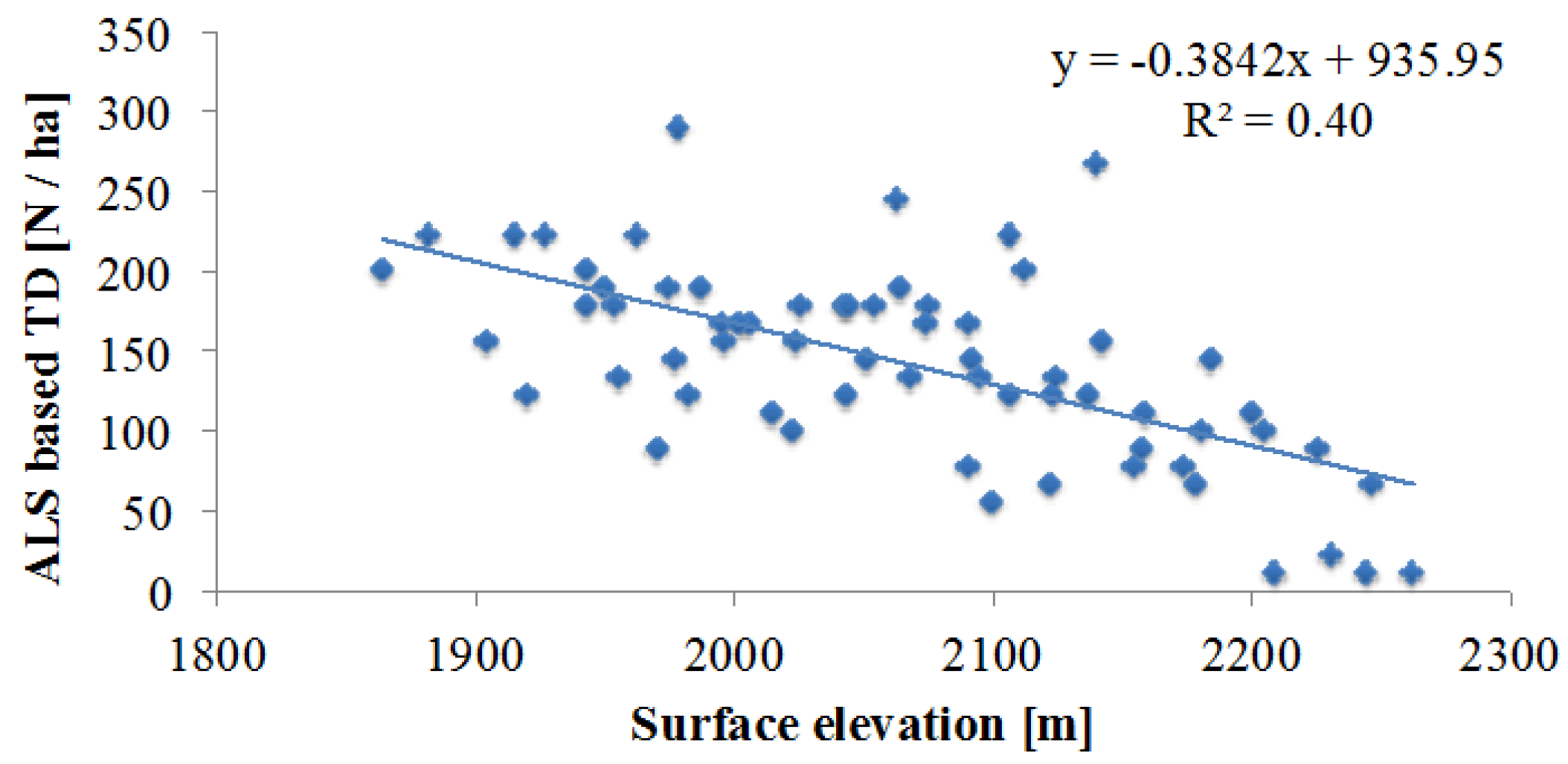
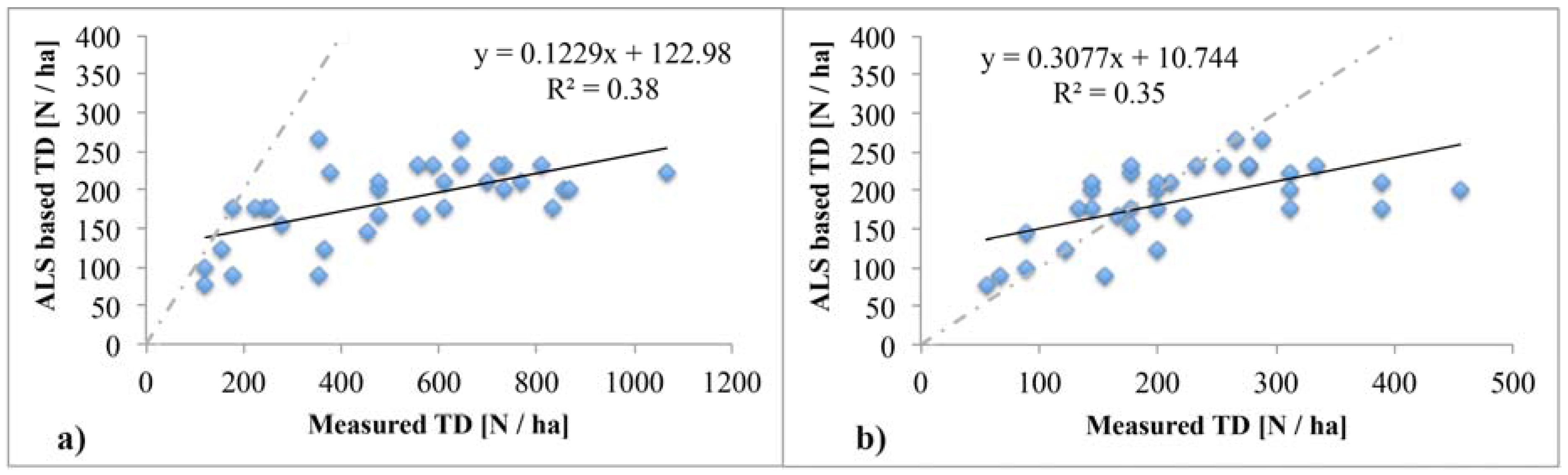
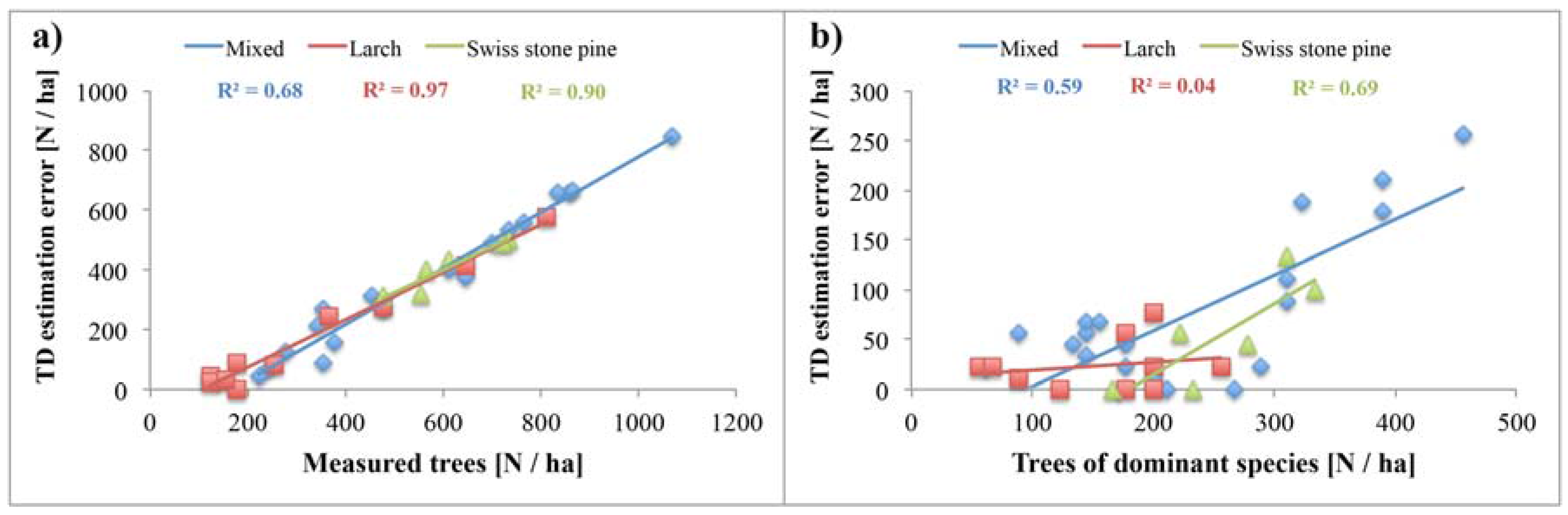
4.1. ALS Based Tree Density Estimation

An example result of the LM-based tree detection is shown in Figure 3. The detection rate was calculated to validate ITD and relates the proportion of detected trees to the number of trees measured in the field (

Table 2. The performance of ITD and for three categories of DBH.

Measured Trees	Detected Trees	Detection Rate [%]
		All DBHs	DBH > 12	DBH > 20	DBH > 30
1598	581	36	43	53	84

). The validation shows a detection rate of 36%, whereby the detection rates ranged from 43% to 85% considering the different DBH categories (cf. Section 2.2).

The results of the ITD were used to calculate the TD per plot, expressed in trees/ha. Considering all trees and DBH classes, TD estimation shows a low accuracy with R² = 0.39 (p < 0.0001), and RMSE = 389 [N/ha]. The accuracy increases by excluding small trees (i.e., DBH > 30 cm) to R² = 0.35 (p = 0.0002) and RMSE = 87 [N/ha] (

Table 3. Agreement of measured and ALS-based tree density estimation. Statistical assessment is based on the root mean square error (RMSE) in trees ha⁻¹ and the coefficient of determination (R²).

Plots	All Trees			DBH > 12			DBH > 20			DBH > 30
	R2	RMSE	RMSE%	R2	RMSE	RMSE%	R2	RMSE	RMSE%	R2	RMSE	RMSE%
All	0.39	389	77	0.40	294	68	0.42	201	57	0.35	87	40
North	0.68	176	56	0.68	124	44	0.74	101	39	0.80	68	33
South	0.52	447	77	0.58	339	69	0.53	229	59	0.27	93	42

). If reference plots are stratified in north- and south-facing plots, the accuracy of TD estimates for all trees increases for north-facing plots (R² = 0.68 (p = 0.006), RMSE = 176 [N/ha]) and remains at a low to moderate level for south-facing plots (R² = 0.52 (p < 0.0001), RMSE = 447 [N/ha]).

The relationship between measured and estimated TD considering all plots and trees is shown in Figure 4a. We observe a general underestimation of TD estimates in particular with increasing amount of trees/ha that is associated with an increasing number of small trees. Even if only large trees are considered (i.e., DBH > 30 cm), there is a tendency for an underestimation of TD in dense canopies (Figure 4b).

The effect of species composition on TD estimates was assessed by stratifying field plots into four classes according to their dominant species. Plots showing individual proportions of less than 60% across all species were considered as mixed [85]. As a result, 18 mixed plots, 10 Larch plots, six Swiss stone pine plots, and one Norway spruce plot were classified. We observe a strong relationship between the amount of trees per ha and the TD estimation error (i.e., the difference between measured trees in the field and estimated trees from ALS data) across species composition (i.e., R² = 0.68 for mixed plots, R² = 0.97 for larch, and R² = 0.90 for Swiss stone pine plots) (Figure 5a). If only large trees are considered (DBH > 30 cm), the TD error tends to be less dependent on TD, but seems to be species-specific (i.e., R² = 0.59 for mixed plots, R² = 0.04 for larch, and R² = 0.69 for Swiss stone pine plots) (Figure 5b).

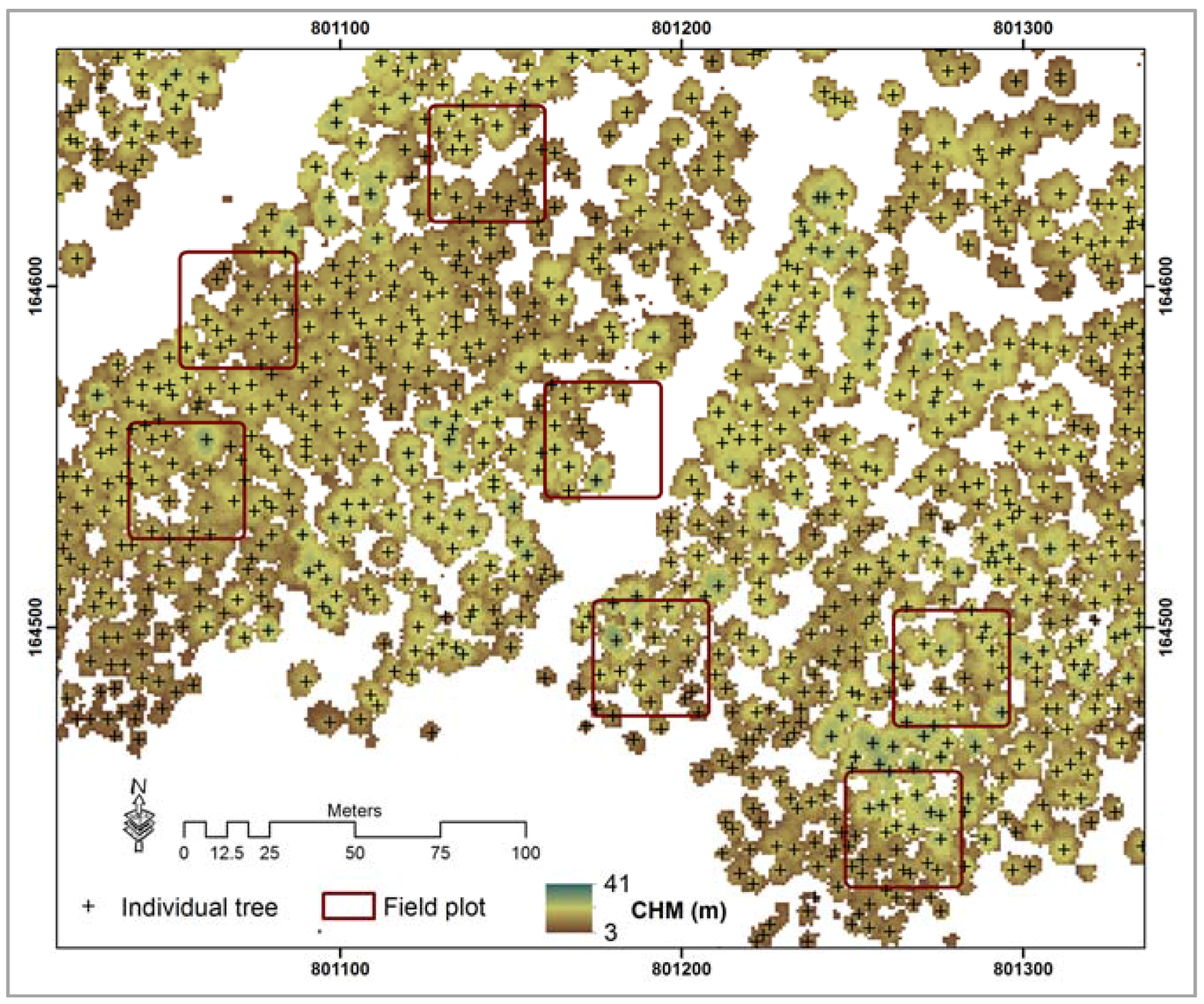
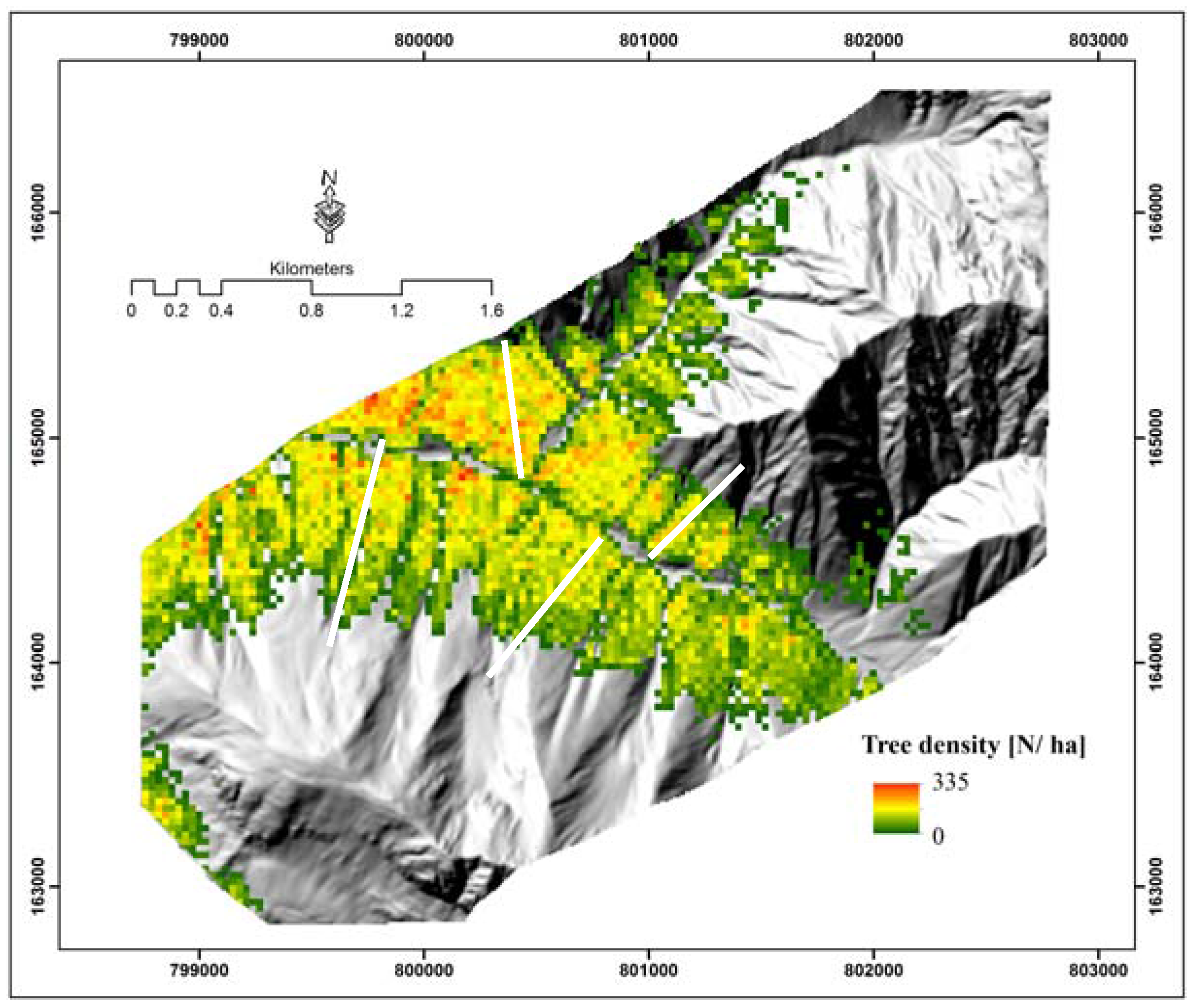
4.2. Spatial Distribution of Tree Density

Identified trees were spatially counted considering a 30 m grid to eventually obtain a thematic TD map of the study area (Figure 6). The mean TD value estimated from ALS data is 184 ± 50 [N/ha], differing 64% from the average value obtained from field surveys (i.e., 507 [N/ha]).

The TD map depicts a higher TD on south-facing slopes compared to north-facing slopes. Further, high TD values dominate at low elevations, and a decreasing TD is obvious with increasing elevation. This negative relationship between TD and surface elevation can be confirmed by the field data (Figure 7a) and by evaluating ALS-based TD values at plot scale (Figure 7b). The assessment of four slope-line parallel transects shows a negative relationship between TD and surface elevation, as well (R² = 0.4 significant at 0.05 (p = 0.00001)) (Figure 8). Further, in situ and ALS-based TD estimates depict that negative relationships are stronger for north-facing (R² = 0.66 significant at 0.05 (p = 0.0043), R² = 0.69 significant at 0.05 (p = 0.0027)) than for south-facing plots (R² = 0.33 significant at 0.05 (p = 0.024), R² = 0.18, not significant at 0.05 (p = 0.11)) (Figure 7). Low p-values (less than 0.05) indicate that changes in measured and estimated TD are statistically related to changes in surface elevation. We found no relationship between the ALS-based TD and changes in surface elevation for south-facing plots.

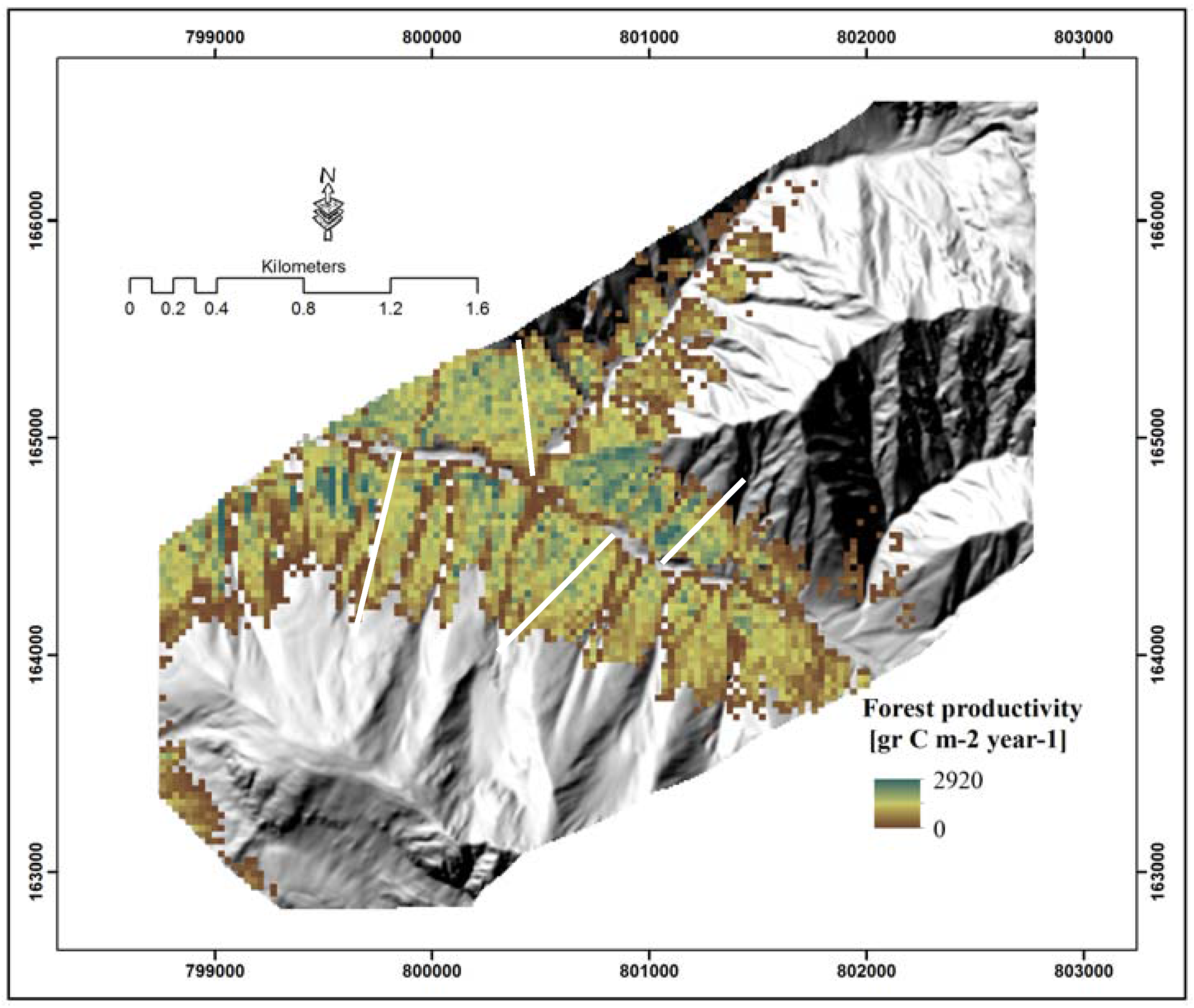
4.3. Spatial Distribution of Forest Productivity

An FP map was calculated by aggregating GPP of sunlit tree crowns to a 30 m grid and normalizing for tree fractional cover (Figure 9). A notable range of FP values is depicted on the map, ranging between 0 and 2920 g C m⁻² year⁻¹. The average FP is 1255 ± 342 g C m⁻² year⁻¹. The map depicts a height gradient of FP with largest productivity values at low elevations and vice versa. However, low FP values frequently occur in the vicinity of a river at the valley bottom.

The relationship between FP and surface elevation was assessed. FP shows a low negative relationship with surface elevation for north-facing plots (R² = 0.31 not significant at 0.05 (p = 0.09)), while no relationship was found for south-facing plots. The analysis at landscape level considering four slope-line parallel transects revealed a more general view on the relationship between FP and surface elevation (see white lines in Figure 9): the findings confirm the plot scale analysis for north-facing slopes while observing a negative relationship (R² = 0.12 significant at 0.05 (p = 0.0034)) (Figure 10) with increasing surface elevation. Our statistical test (p-value) indicates that changes in the surface elevation are associated with changes in the FP. It must be noted that FP generally shows a moderate negative relationship with surface elevation. The lower FP close to a river at the valley bottom, however, determines a bell shaped relationship with surface elevation, and causes the relatively low R² when a linear relationship is considered.

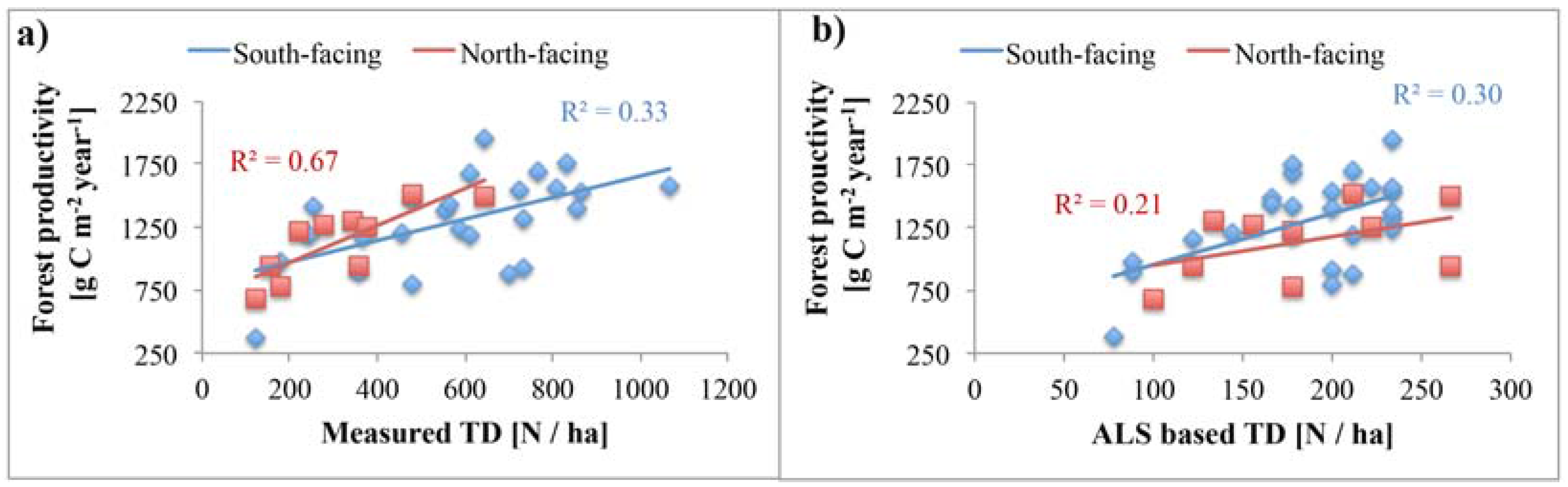
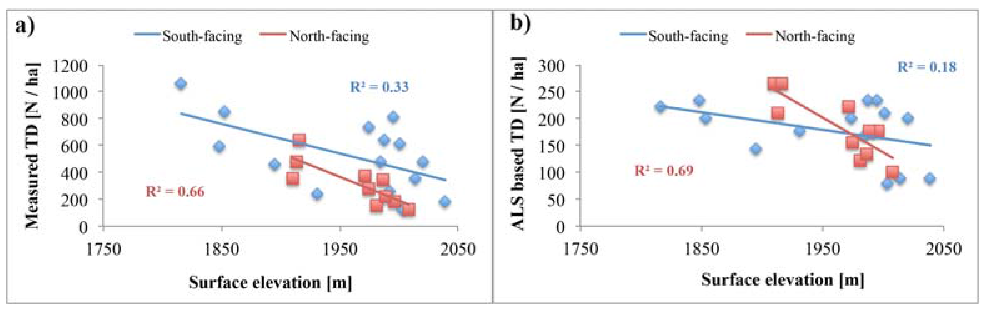
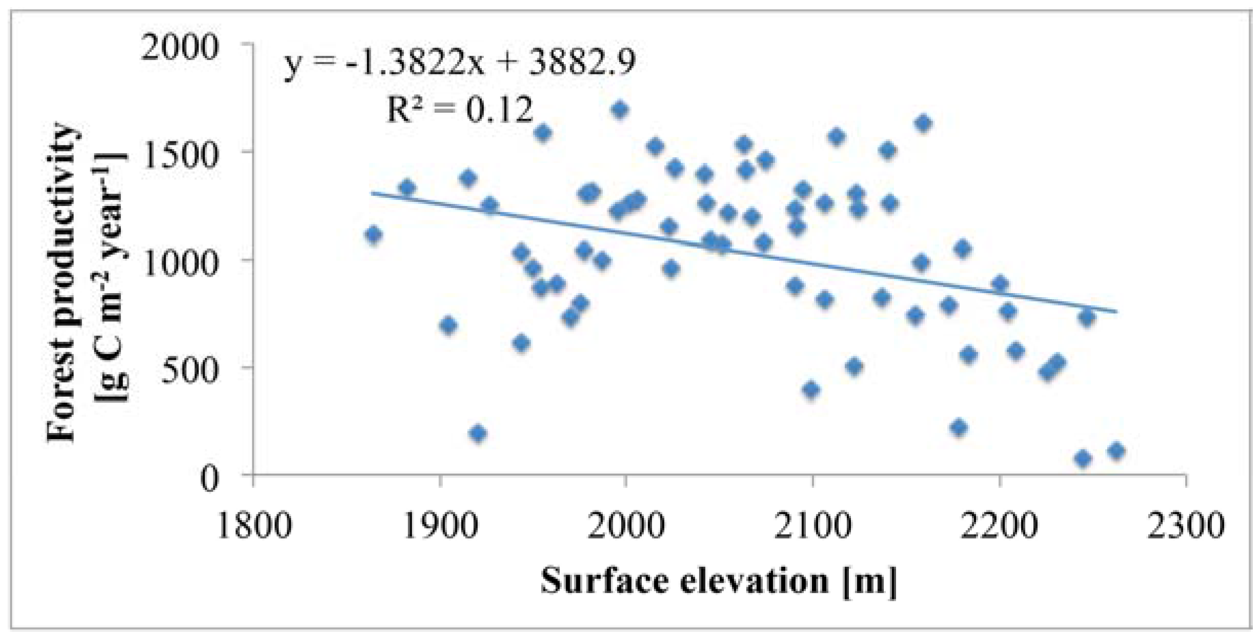
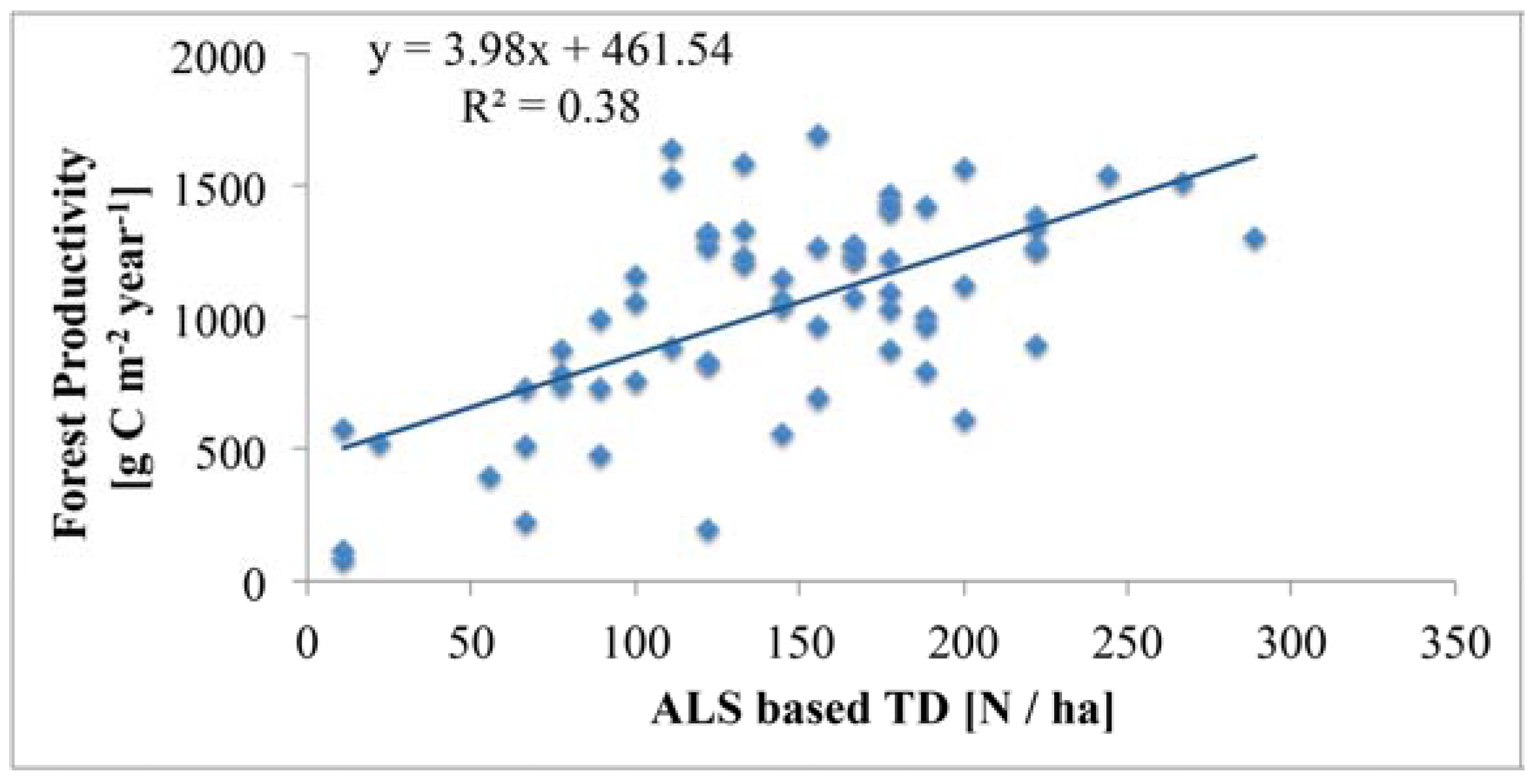
4.4. Relationship of Tree Density with Forest Productivity

The relationship between TD and FP from spatially aggregated APEX data at plot level is shown in Figure 11. The relationships are moderate and positive across exposition (i.e., north- and south-facing slopes) and ITD estimation methods (i.e., field and ALS based) (R² between 0.21 not significant at 0.05 (p = 0.182), and 0.67 significant at 0.05 (p = 0.004)). Plot level results are confirmed at landscape level while we found a positive relationship between TD and FP of R² = 0.38 significant at 0.05 (p = 0.00001) (Figure 12).

5. Discussion

5.1. Reliability of Tree Density Retrieval

We assessed an LM-based approach in combination with ALS data to estimate TD in a heterogeneous alpine forest. Considering all trees with a DBH threshold >5 cm, a moderate accuracy (i.e., R² of 0.39) with a substantial underestimation (RMSE of 389 trees per ha, rRMSE of 70%) was achieved in the heterogeneous alpine environment. This result is in agreement with Næsset & Bjerknes [5], who found a relationship between estimated and reference TD of R² = 0.40 in a coniferous forest in Norway. Yet, other studies evaluating the TD estimation accuracy report R² values ranging from 0.40 to 0.85 [5,25,30,41,75,86]. Jaskierniak et al. [87] indicate TD estimation accuracies ranging between 40–70% considering several studies carried out in Scandinavian and European forests.

The consideration of trees with larger DBHs decreases uncertainties in estimated TD (i.e., R² increases up to 0.80, RMSE decreases to 68 trees per ha, rRMSE of 40%). This finding corresponds to results documented by Lefsky et al. [30], who found a strong relationship for ALS-based TD estimates considering a DBH > 100 cm (R² = 0.85). Casas et al. [88] report a TD estimation accuracy of 87% for trees with a DBH > 30 cm. The dependency of the TD estimation accuracy on DBH indicates a sensitivity issue of the applied ALS-LM approach, while mainly small trees cannot be differentiated and reliably identified. In fact, we observe better TD estimates using a CHM with higher resolution, which is in agreement with Tesfamichael et al. [3].

Our results suggest that forest structure and species composition affect the TD retrieval accuracy. Indeed, crown shape and canopy density determine the success of the LM approach, which basically exploits the morphology of ALS-derived CHMs [41,76]. If tree crowns are flat or show multiple main branches, the LM approach is likely to fail. Several studies have demonstrated that forest structure strongly affects the capability of ALS data to characterize forest properties [40,41,89,90]. In particular, the occurrence of multi-stemmed trees, as caused by a complex mix of environmental factors, disturbances and historical management [91], impacts the detection of individual trees [26,90,92,93]. Further, in the presence of steep slopes, a spatial misplacement between crown top and stem position on ground is likely and additionally affects the accuracy of ITDs [94,95].

Structural effects obviously cause ITD and eventually TD estimates to be dependent on actual species. Physiological considerations add another complication and cause TD estimates to be dependent on species composition, in particular in multi-layered heterogeneous forests. European larch, for example, is largely abundant in our study site and a shade intolerant and fast growing species. Therefore, larch trees form and dominate the upper forest canopy layer [53], covering other more shade-tolerant and slow-growing species underneath, e.g., Swiss stone pine and Norway spruce. The multi-layering hides trees and thus impacts the TD estimation accuracy. We observed a dependency of TD estimates on surface orientation, i.e., north- and south-facing. TD estimates were less accurate for south-facing slopes compared to those on north-facing slopes. Since south-facing areas are characterized by a higher TD and the occurrence of multiple-stemmed trees, the lower TD estimation accuracy can be attributed to structural aspects.

Optimized ALS data acquisition allows overcoming certain issues discussed above, eventually yielding improved ITD and TD estimates. One option would be the use of multi-temporal ALS data (i.e., leaf-on and leaf-off) [96]. Since Larch is a deciduous conifer tree, leaf-off data would allow an improvement in the detection of trees present in lower canopy layers. Further, employing ALS data with higher point density could increase the chance to capture more echo returns vertically across the forest canopy. Vauhkonen et al. [41], for example, found that an ITD approach performs best with point densities of 5–10 pts/m² or by using full waveform data [24,96]. Further, a stratified field sampling as implemented in our study is also important for facilitating the data analysis. Besides distributing potential reference plots along elevation gradients, a stratification for exposition, tree age and size [5], tree species, and species composition [90] has been found to be crucial in providing a representative set of reference data for remote sensing-based analysis. Such considerations are also recommended in order to optimize forest inventories if time-consuming field surveys are needed.

5.2. Reliability of Forest Productivity Retrieval

We approximated FP with GPP. Estimates of GPP from optical EO data are typically based on two approaches: using vegetation greenness to indicate potential photosynthetic activity; or measurements directly related to actual photosynthesis such as SIF. The use of SIF would be the preferred option, but the spectral resolution of the available APEX data is not optimized for SIF retrievals. Although SIF retrievals from APEX data have been successfully demonstrated [49], retrievals in topographically complex environments are likely to be uncertain. Hence, we applied a greenness-based approach in this study. Such simple empirical approaches are frequently used to estimate forest GPP with optical remote sensing data. The approach by Hashimoto et al. [79], as applied in this study, relies on the EVI to constrain estimates of GPP. Previous studies have demonstrated that the sole use of the EVI can predict GPP as accurate as the current version of the MOD17 algorithm [97,98]. Comparisons of modeled GPP and the MOD17 GPP product indicate, on the one hand, that the modeled mean GPP is about 26% lower than the MOD17 GPP product. On the other hand, Heinsch et al. [99] report that the MOD17 GPP product tends to overestimate flux tower-based GPP by 20–30%. Such uncertainties can be attributed to the fact that all these approaches rely on vegetation indices representing the greenness of vegetation, and therefore the potential rather than actual photosynthetic activity. Further, we took a single observation in time in combination with the empirical model from Hashimoto to obtain annual GPP. Since the forest ecosystem shows a pronounced phenological cycle, estimated GPP are likely to be overestimated. In fact, Zielis et al. [100] and Wolf et al. [101] report maximum GPP values of 5 g C m⁻² day⁻¹ for a Norway spruce forest close to Davos, Switzerland, that is comparable to our observation taken at the peak season. Scaling their flux tower-based GPP estimates to annual values results in roughly 1000 g C m⁻² year⁻¹, while we observed average values of 1255 ± 342 g C m⁻² year⁻¹, confirming the expected overestimation of GPP when using a single snapshot in combination with the EVI approach. However, GPP estimates based on vegetation greenness provide first meaningful insights into the spatio-temporal patterns of GPP in complex landscapes. The use of time series for the new EO approach involving SIF allows the stated limitations to be overcome, since SIF is the most direct measurement of photosynthetic activity. The measurement of SIF can be considered mature, but the use of SIF to constrain estimates of GPP still requires further attention. Nevertheless, first studies demonstrate and suggest improved SIF-based GPP estimates across different scales, i.e., field scale [102], regional scale [49,103], and global scale [104,105,106], as well as theoretically [107].

5.3. Topography Effects on Tree Density and Forest Productivity

We observed a negative relationship between TD and surface elevation. This trend is coherent across the used TD estimates (i.e., ALS- or in situ-based) and scales (i.e., plot, landscape) and is in line with results documented in the literature [108]. The decreasing TD with increasing surface elevation can be associated with the availability of resources (i.e., temperature, water, nutrients) and the competition for them among trees. Additionally, mechanical pressure (e.g., storm damages), in combination with slow growing rates, could explain the topography impact on TD. Our results show stronger negative trends for north-facing slopes (i.e., R² ~ 0.6 with a negative slope) than south-facing slopes (i.e., R² ~ 0.2–0.3 with a negative slope) at plot scale. This finding suggests that, and provides further evidence that, in subalpine forest ecosystems resource availability strongly determines TD, since north-facing slopes are generally colder and thus show even larger temperature gradients that are less favorable for tree growth.

TD and FP are positively related across scales. This finding is expected, since a co-variance of both variables with height-dependent gradients of growth-limiting factors and eventually canopy density exists. Our findings show stronger positive dependency for north-facing plots (i.e., R² ~ 0.6) than south-facing plots, confirmed at landscape scale as well (showing a moderate dependency with an R² ~ 0.3). Therefore, we may conclude that the more trees, the higher the total productivity of a forested area, and vice versa. Associated with this is the negative relationship between FP and surface elevation. This finding is in line with an early and often-cited study by Whittaker et al. [109] and other studies [108,109,110,111]. As for TD, the negative relationship is plausible for the investigated alpine environment, since surface elevation dependent gradients of growth-limiting factors (e.g., nutrients, temperature, water) are likely to affect tree growth. Paulsen et al. [108], for example, conclude that a reduction of tree productivity towards the upper tree line is directly associated to decreasing temperature. We also observed a strong decline of FP in lower elevations in the vicinity of a river in the valley bottom. Causes for the reduced productivity are related to steep terrain and unfortunate soil conditions (rock, nutrient limitation) due to flooding events of the river.

However, it must be noted that the use of simple vegetation indices as a proxy for GPP, in combination with difficulties in describing the radiative transfer of complex canopies (i.e., the fractions of direct and diffuse irradiance components) [84], likely contributes to uncertainty in the FP estimates. Further analyses considering larger elevation gradients and more appropriate remote sensing approaches (e.g., SIF) are suggested in order to yield a more general view on forest growth patterns in alpine environments and underlying causes such as resource limitations.

6. Conclusions

Forest inventories seek to measure the quantity and quality of a forest ecosystem, and form the foundation of forest planning and forest policy. The focus of the traditional forest inventory was on obtaining information on structural attributes, such as basal area, tree height, and number of trees. Recently, modern forest inventories have emphasized gaining information, not only on structural attributes, but also by addressing forest-functional attributes in order to understand the functioning mechanisms of forest ecosystems [112]. In addition, making full use of new technologies is one of the challenges that modern forest inventories face today. We aimed to evaluate the capability of two new technologies, ALS and IS, in characterizing a heterogeneous forest ecosystem.

We conclude that estimates of TD in heterogeneous alpine landscapes challenge current technology and analytical approaches. Tree and canopy structure are the primary determinants of the success of TD estimates, which are, in addition, dependent on species and canopy species composition. For deciduous trees, for example, the applied local maximum approach has strong limitations, as a detection of the treetop is not completely unambiguous (cf. Koch et al., 2006 [24]). In terms of the structure, the occurrence of multi-stem trees sharing a common canopy needs to be considered. Further, ALS-based approaches show a sensitivity limit, in particular, when identifying small trees. Specific sampling schemes, e.g., multi-temporal ALS data acquisition with high point density, will partly allow an increase in the sensitivity and accuracy of TD estimation. Further, simple empirical approaches provide sufficient accuracy to reveal first insights into interrelationships between FP and topography effects. More sophisticated and mechanistic approaches are, however, required to yield in-depth knowledge. We conclude that airborne laser scanning and imaging spectroscopy and their combination provide crucial technology for assessing TD and FP for less heterogeneous stands, e.g., north-facing forested areas, at relevant ecological scales.

We can confirm the existing theory that heterogeneous alpine forests are characterized by positive relationships between FP and TD, mainly due to a significant co-variance of both variables with elevation-dependent gradients of growth-limiting factors. We suggest extending this analysis by considering a wider range of forest types, landscape heterogeneity, topography, resource gradients and assessing the role of other forest structural attributes, e.g., canopy height and canopy cover, on FP. This ultimately allows the gaining of a deeper understanding of TD and FP variability and interrelationships across landscapes.

References

1. Johnson, P.E.; Shifley, S.R.; Rogers, R. The Ecology and Silviculture of Oaks; CABI: Wallingford, UK, 2009. [Google Scholar]
2. Fatehi, P.; Damm, A.; Schaepman, M.E.; Kneubühler, M. Estimation of alpine forest structural variables from imaging spectrometer data. Remote Sens. 2015, 7, 16315–16338. [Google Scholar] [CrossRef]
3. Tesfamichael, S.G.; Ahmed, F.; van Aardt, J.A.N.; Blakeway, F. A semi-variogram approach for estimating stems per hectare in Eucalyptus grandis plantations using discrete-return lidar height data. For. Ecol. Manag. 2009, 258, 1188–1199. [Google Scholar] [CrossRef]
4. Houghton, R.A.; Hall, F.; Goetz, S.J. Importance of biomass in the global carbon cycle. J. Geophys. Res. Biogeosciences 2009, 114, 1–13. [Google Scholar] [CrossRef]
5. Næsset, E.; Bjerknes, K.-O. Estimating tree heights and number of stems in young forest stands using airborne laser scanner data. Remote Sens. Environ. 2001, 78, 328–340. [Google Scholar] [CrossRef]
6. Capers, R.S.; Chazdon, R.L.; Brenes, A.R.; Alvarado, B.V. Successional dynamics of woody seedling communities in wet tropical secondary forests. J. Ecol. 2005, 93, 1071–1084. [Google Scholar] [CrossRef]
7. Sproull, G.J.; Adamus, M.; Bukowski, M.; Krzyżanowski, T.; Szewczyk, J.; Statwick, J.; Szwagrzyk, J. Tree and stand-level patterns and predictors of Norway spruce mortality caused by bark beetle infestation in the Tatra Mountains. For. Ecol. Manag. 2015, 354, 261–271. [Google Scholar] [CrossRef]
8. Pretzsch, H. Forest Dynamics, Growth, and Yield; Springer: Berlin/Heidelberg, Germany, 2009. [Google Scholar]
9. Skovsgaard, J.P.; Vanclay, J.K. Forest site productivity: A review of the evolution of dendrometric concepts for even-aged stands. Forestry 2008, 81, 13–31. [Google Scholar] [CrossRef]
10. Rayan, M.G.; Binkley, D.; Fownes, J.H. Age-Related Decline in Forest Productivity: Pattern and Process. Adv. Ecol. Res. 1997, 27, 213–262. [Google Scholar]
11. Goetz, S.J.; Prince, S.D. Remote sensing of net primary production in boreal forest stands. Agric. For. Meteorol. 1996, 78, 149–179. [Google Scholar] [CrossRef]
12. Bontemps, J.-D.; Bouriaud, O. Predictive approaches to forest site productivity: Recent trends, challenges and future perspectives. Forestry 2013, 87, 109–128. [Google Scholar] [CrossRef]
13. Maselli, F.; Papale, D.; Puletti, N.; Chirici, G.; Corona, P. Combining remote sensing and ancillary data to monitor the gross productivity of water-limited forest ecosystems. Remote Sens. Environ. 2009, 113, 657–667. [Google Scholar] [CrossRef]
14. Crowther, T.W.; Glick, H.B.; Covey, K.R.; Bettigole, C.; Maynard, D.S.; Thomas, S.M.; Smith, J.R.; Hintler, G.; Duguid, M.C.; Amatulli, G.; et al. Mapping tree density at a global scale. Nature 2015, 525, 201–205. [Google Scholar] [CrossRef] [PubMed]
15. Belote, R.T.; Prisley, S.; Jones, R.H.; Fitzpatrick, M.; de Beurs, K. Forest productivity and tree diversity relationships depend on ecological context within mid-Atlantic and Appalachian forests (USA). For. Ecol. Manag. 2011, 261, 1315–1324. [Google Scholar] [CrossRef]
16. Bolton, D.K.; Coops, N.C.; Wulder, M.A. Measuring forest structure along productivity gradients in the Canadian boreal with small-footprint Lidar. Environ. Monit. Assess. 2013, 185, 6617–6634. [Google Scholar] [CrossRef] [PubMed]
17. Lefsky, M.A.; Cohen, W.B.; Parker, G.G.; Harding, D.J. Lidar Remote Sensing for Ecosystem Studies. Bioscience 2002, 52, 19–30. [Google Scholar] [CrossRef]
18. Liu, J.; Yunhong, T.; Slik, J.W.F. Topography related habitat associations of tree species traits, composition and diversity in a Chinese tropical forest. For. Ecol. Manag. 2014, 330, 75–81. [Google Scholar] [CrossRef]
19. Körner, C.; Farquhar, G.D.; Roksandic, Z. A global Survey of carbon Isotope Discrimination in Plants from High Altitude. Oecologia 2009, 74, 623–632. [Google Scholar] [CrossRef] [PubMed]
20. Asner, G.P.; Martin, R.E.; Anderson, C.B.; Kryston, K.; Vaughn, N.; Knapp, D.E.; Bentley, L.P.; Shenkin, A.; Salinas, N.; Sinca, F.; et al. Scale dependence of canopy trait distributions along a tropical forest elevation gradient. New Phytol. 2017, 214, 973–988. [Google Scholar] [CrossRef] [PubMed]
21. Coops, N.C.; Morsdorf, F.; Schaepman, M.E.; Zimmermann, N.E. Characterization of an alpine tree line using airborne LiDAR data and physiological modeling. Glob. Chang. Biol. 2013, 19, 3808–3821. [Google Scholar] [CrossRef] [PubMed]
22. Hyyppä, J.; Hyyppä, H.; Inkinen, M.; Engdahl, M.; Linko, S.; Zhu, Y.-H. Accuracy comparison of various remote sensing data sources in the retrieval of forest stand attributes. For. Ecol. Manag. 2000, 128, 109–120. [Google Scholar] [CrossRef]
23. Maselli, F.; Chiesi, M.; Mura, M.; Marchetti, M.; Corona, P.; Chirici, G. Combination of optical and LiDAR satellite imagery with forest inventory data to improve wall-to-wall assessment of growing stock in Italy. Int. J. Appl. Earth Obs. Geoinf. 2014, 26, 377–386. [Google Scholar] [CrossRef]
24. Koch, B.; Heyder, U.; Weinacker, H. Detection of Individual Tree Crowns in Airborne Lidar Data. Photogramm. Eng. Remote Sens. 2006, 72, 357–363. [Google Scholar] [CrossRef]
25. Hall, S.A.; Burke, I.C.; Box, D.O.; Kaufmann, M.R.; Stoker, J.M. Estimating stand structure using discrete-return lidar: An example from low density, fire prone ponderosa pine forests. For. Ecol. Manag. 2005, 208, 189–209. [Google Scholar] [CrossRef]
26. Maltamo, M.; Eerikäinen, K.; Pitkänen, J.; Hyyppä, J.; Vehmas, M. Estimation of timber volume and stem density based on scanning laser altimetry and expected tree size distribution functions. Remote Sens. Environ. 2004, 90, 319–330. [Google Scholar] [CrossRef]
27. Hudak, A.T.; Crookston, N.L.; Evans, J.S.; Falkowski, M.J.; Smith, A.M.; Gessler, P.E.; Morgan, P. Regression modeling and mapping of coniferous forest basal area and tree density from discrete-return lidar and multispectral satellite data. Can. J. Remote Sens. 2006, 32, 126–138. [Google Scholar] [CrossRef]
28. Sivanpillai, R.; Smith, C.T.; Srinivasan, R.; Messina, M.G.; Wu, X.B. Estimation of managed loblolly pine stand age and density with Landsat ETM+ data. For. Ecol. Manag. 2006, 223, 247–254. [Google Scholar] [CrossRef]
29. Cho, M.A.; Skidmore, A.K.; Sobhan, I. Mapping beech (Fagus sylvatica L.) forest structure with airborne hyperspectral imagery. Int. J. Appl. Earth Obs. Geoinf. 2009, 11, 201–211. [Google Scholar] [CrossRef]
30. Lefsky, M.A.; Cohen, W.B.; Acker, S.A.; Parker, G.G.; Spies, T.A.; Harding, D. Lidar Remote Sensing of the Canopy Structure and Biophysical Properties of Douglas-Fir Western Hemlock Forests. Remote Sens. Environ. 1999, 70, 339–361. [Google Scholar] [CrossRef]
31. Brosofske, K.D.; Froese, R.E.; Falkowski, M.J.; Banskota, A. A Review of Methods for Mapping and Prediction of Inventory Attributes for Operational Forest Management. For. Sci. 2014, 60, 733–756. [Google Scholar] [CrossRef]
32. Leiterer, R.; Mücke, W.; Morsdorf, F.; Hollaus, M.; Pfeifer, N.; Schapeman, M.E. Operational forest structure monitoring using airborne laser scanning. Photogramm. Fernerkund. Geoinf. 2013, 3, 173–184. [Google Scholar] [CrossRef]
33. Maltamo, M.; Næsset, E.; Vauhkonen, J. Forestry Applications of Airborne Laser Scanning: Concepts and Case Studies; Springer: Dordrecht, The Netherlands, 2014. [Google Scholar]
34. Wulder, M.A.; Coops, N.C.; Hudak, A.T.; Morsdorf, F.; Nelson, R.; Newnham, G.; Vastaranta, M. Status and prospects for LiDAR remote sensing of forested ecosystems. Can. J. Remote Sens. 2013, 39, 1–5. [Google Scholar] [CrossRef]
35. Hyyppä, J.; Yu, X.; Hyyppä, H.; Vastaranta, M.; Holopainen, M.; Kukko, A.; Kaartinen, H.; Jaakkola, A.; Vaaja, M.; Koskinen, J.; et al. Advances in Forest Inventory Using Airborne Laser Scanning. Remote Sens. 2012, 4, 1190–1207. [Google Scholar] [CrossRef]
36. Næsset, E. Determination of mean tree height of forest stands using airborne laser scanner data. ISPRS J. Photogramm. Remote Sens. 1997, 52, 49–56. [Google Scholar] [CrossRef]
37. White, J.C.; Wulder, M.A.; Varhola, A.; Vastaranta, M.; Coops, N.C.; Cook, B.D.; Pitt, D.; Woods, M. A best practices guide for generating forest inventory attributes from airborne laser scanning data using an area-based approach. For. Chron. 2013, 89, 722–723. [Google Scholar] [CrossRef]
38. Tompalski, P.; Coops, N.C.; White, J.C.; Wulder, M.A. Enriching ALS-Derived Area-Based Estimates of Volume through Tree-Level Downscaling. Forests 2015, 6, 2608–2630. [Google Scholar] [CrossRef]
39. Roberts, S.D.; Dean, T.J.; Evans, D.L.; McCombs, J.W.; Harrington, R.L.; Glass, P.A. Estimating individual tree leaf area in loblolly pine plantations using LiDAR-derived measurements of height and crown dimensions. For. Ecol. Manag. 2005, 213, 54–70. [Google Scholar] [CrossRef]
40. Vastaranta, M.; Saarinen, N.; Kankare, V.; Holopainen, M.; Kaartinen, H.; Hyyppä, J.; Hyyppä, H. Multisource Single-Tree Inventory in the Prediction of Tree Quality Variables and Logging Recoveries. Remote Sens. 2014, 6, 3475–3491. [Google Scholar] [CrossRef]
41. Vauhkonen, J.; Ene, L.; Gupta, S.; Heinzel, J.; Holmgren, J.; Pitkanen, J.; Solberg, S.; Wang, Y.; Weinacker, H.; Hauglin, K.M.; et al. Comparative testing of single-tree detection algorithms under different types of forest. Forestry 2012, 85, 27–40. [Google Scholar] [CrossRef]
42. Kaartinen, H.; Hyyppä, J.; Yu, X.; Vastaranta, M.; Hyyppä, H.; Kukko, A.; Holopainen, M.; Heipke, C.; Hirschmugl, M.; Morsdorf, F.; et al. An International Comparison of Individual Tree Detection and Extraction Using Airborne Laser Scanning. Remote Sens. 2012, 4, 950–974. [Google Scholar] [CrossRef]
43. Monteith, J.L.; Moss, C.J. Climate and the efficiency of crop production in Britain [and discussion]. Philos. Trans. R Soc. Lond. B Biol. Sci. 1977, 281, 227–294. [Google Scholar] [CrossRef]
44. Waring, R.H.; Coops, N.C.; Fan, W.; Nightingale, J.M. MODIS enhanced vegetation index predicts tree species richness across forested ecoregions in the contiguous U.S.A. Remote Sens. Environ. 2006, 103, 218–226. [Google Scholar] [CrossRef]
45. Hilker, T.; Coops, N.C.; Wulder, M.A.; Black, T.A.; Guy, R.D. The use of remote sensing in light use efficiency based models of gross primary production: A review of current status and future requirements. Sci. Total Environ. 2008, 404, 411–423. [Google Scholar] [CrossRef] [PubMed]
46. Turner, D.P.; Ritts, W.D.; Cohen, W.B.; Maeirsperger, T.K.; Gower, S.T.; Kirschbaum, A.A.; Running, S.W.; Zhao, M.; Wofsy, S.C.; Dunn, A.L.; et al. Site-level evaluation of satellite-based global terrestrial gross primary production and net primary production monitoring. Glob. Chang. Biol. 2005, 11, 666–684. [Google Scholar] [CrossRef]
47. Coops, N.C.; Ferster, C.J.; Waring, R.H.; Nightingale, J. Comparison of three models for predicting gross primary production across and within forested ecoregions in the contiguous United States. Remote Sens. Environ. 2009, 113, 680–690. [Google Scholar] [CrossRef]
48. Schimel, D.; Pavlick, R.; Fisher, J.B.; Asner, G.P.; Saatchi, S.; Townsend, P.A.; Miller, C.; Frankenberg, C.; Hibbard, K.; Cox, P. Observing terrestrial ecosystems and the carbon cycle from space. Glob. Chang. Biol. 2015, 21, 1762–1776. [Google Scholar] [CrossRef] [PubMed]
49. Damm, A.; Guanter, L.; Paul-Limoges, E.; van der Tol, C.; Hueni, A.; Buchmann, N.; Eugster, W.; Ammann, C.; Schaepman, M.E. Far-red sun-induced chlorophyll fluorescence shows ecosystem-specific relationships to gross primary production: An assessment based on observational and modeling approaches. Remote Sens. Environ. 2015, 166, 91–105. [Google Scholar] [CrossRef]
50. MeteoSwiss IDAweb. The Data Portal of MeteoSwiss for Research and Teaching. Available online: http://www.meteoschweiz.admin.ch/web/de/services/datenportal/idaweb.html (accessed on 3 November 2013).
51. Hill, A.; Breschan, J.; Mandallaz, D. Accuracy Assessment of Timber Volume Maps Using Forest Inventory Data and LiDAR Canopy Height Models. Forests 2014, 5, 2253–2275. [Google Scholar] [CrossRef]
52. Schweiger, A.K.; Schütz, M.; Anderwald, P.; Schaepman, M.E.; Kneubühler, M.; Haller, R.; Risch, A.C. Foraging ecology of three sympatric ungulate species—Behavioural and resource maps indicate differences between chamois, ibex and red deer. Mov. Ecol. 2015, 3, 1–12. [Google Scholar] [CrossRef] [PubMed]
53. Risch, A.C.; Nagel, L.M.; Martin, S.; KrÜsi, B.O.; Kienast, F.; Bugmman, H. Structure and Long-Term Development of Subalpine Pinus montana Miller and Pinus cembra L. Forests in the Central European Alps. Forstwiss. Cent. 2003, 122, 219–230. [Google Scholar] [CrossRef]
54. Kangas, A.; Maltamo, M. Forest Inventory Methodology and Applications; Springer: Berlin, Germany, 2006. [Google Scholar]
55. Da Cunha, T.A.; Finger, C.A.G.; Hasenauer, H. Tree basal area increment models for Cedrela, Amburana, Copaifera and Swietenia growing in the Amazon rain forests. For. Ecol. Manag. 2016, 365, 174–183. [Google Scholar] [CrossRef]
56. Leboeuf, A.; Beaudoin, A.; Fournier, R.A.; Guindon, L.; Luther, J.; Lambert, M. A shadow fraction method for mapping biomass of northern boreal black spruce forests using QuickBird imagery. Remote Sens. Environ. 2007, 110, 488–500. [Google Scholar] [CrossRef]
57. Risch, A.C.; Jurgensen, M.F.; Page-Dumroese, D.S.; Wildi, O.; Schütz, M. Long-term development of above-and below-ground carbon stocks following land-use change in subalpine ecosystems of the Swiss National Park. J. For. 2008, 1602, 1590–1602. [Google Scholar] [CrossRef]
58. Pretzsch, H. Canopy space filling and tree crown morphology in mixed-species stands compared with monocultures. For. Ecol. Manag. 2014, 327, 251–264. [Google Scholar] [CrossRef]
59. Paulsen, J.; Körner, C. GIS-Analysis of Tree-Line Elevation in the Swiss Alps Suggests no Exposure Effect. J. Veg. Sci. 2011, 12, 817–824. [Google Scholar] [CrossRef]
60. Schaepman, M.E.; Jehle, M.; Hueni, A.; D’Odorico, P.; Damm, A.; Weyermann, J.; Schneider, F.D.; Laurent, V.; Popp, C.; Seidel, F.C.; et al. Advanced radiometry measurements and Earth science applications with the Airborne Prism Experiment (APEX). Remote Sens. Environ. 2015, 158, 207–219. [Google Scholar] [CrossRef]
61. Schläpfer, D.; Richter, R. Geo-atmospheric processing of airborne imaging spectrometry data. Part 1: Parametric orthorectification. Int. J. Remote Sens. 2002, 23, 2609–2630. [Google Scholar] [CrossRef]
62. Richter, R.; Schläpfer, D. Geo-atmospheric processing of airborne imaging spectrometry data. Part 2: Atmospheric/topographic correction. Int. J. Remote Sens. 2002, 23, 2631–2649. [Google Scholar] [CrossRef]
63. Schaepman-Strub, G.; Schaepman, M.E.; Painter, T.H.; Dangel, S.; Martonchik, J.V. Reflectance quantities in optical remote sensing—Definitions and case studies. Remote Sens. Environ. 2006, 103, 27–42. [Google Scholar] [CrossRef]
64. Berk, A.; Anderson, G.P.; Acharya, P.K.; Bernstein, L.S.; Muratov, L.; Lee, J.; Fox, M.J.; Alder-Golden, S.M.; Chetwynd, J.H.; Hoke, M.L.; et al. MODTRAN5: A reformulated atmospheric band model with auxiliary species and practical multiple scattering options. In Proceedings of the Society of Photo-Optical Instrumentation Engineer, International Society for Optics and Photonics, Bellingham, WA, USA, 20 January 2005; pp. 662–667. [Google Scholar]
65. Wagner, W.; Hollaus, M.; Briese, C.; Ducic, V. 3D vegetation mapping using small-footprint full-waveform airborne laser scanners. Int. J. Remote Sens. 2008, 29, 1433–1452. [Google Scholar] [CrossRef]
66. RIEGL Products. Airborne Scanning Datasheets. Available online: http://www.riegl.com (accessed on 4 June 2015).
67. Mallet, C.; Bretar, F. Full-waveform topographic lidar: State-of-the-art. ISPRS J. Photogramm. Remote Sens. 2009, 64, 1–16. [Google Scholar] [CrossRef]
68. Hollaus, M.; Wagner, W.; Eberhöfer, C.; Karel, W. Accuracy of large-scale canopy heights derived from LiDAR data under operational constraints in a complex alpine environment. ISPRS J. Photogramm. Remote Sens. 2006, 60, 323–338. [Google Scholar] [CrossRef]
69. Jakubowski, M.K.; Guo, Q.; Kelly, M. Tradeoffs between lidar pulse density and forest measurement accuracy. Remote Sens. Environ. 2013, 130, 245–253. [Google Scholar] [CrossRef]
70. Brassel, P.; Lischke, H. Swiss National Forest Inventory: Methods and Models of the Second Assessment; WSL Swiss Federral Research Institute: Birmensdorf, Switzerland, 2001. [Google Scholar]
71. Kankare, V.; Vastaranta, M.; Holopainen, M.; Räty, M.; Yu, X.; Hyyppä, J.; Hyyppä, H.; Alho, P.; Viitala, R. Retrieval of Forest Aboveground Biomass and Stem Volume with Airborne Scanning LiDAR. Remote Sens. 2013, 5, 2257–2274. [Google Scholar] [CrossRef]
72. Leckie, D. Stand delineation and composition estimation using semi-automated individual tree crown analysis. Remote Sens. Environ. 2003, 85, 355–369. [Google Scholar] [CrossRef]
73. Katoh, M.; Gougeon, F.A. Improving the Precision of Tree Counting by Combining Tree Detection with Crown Delineation and Classification on Homogeneity Guided Smoothed High Resolution (50 cm) Multispectral Airborne Digital Data. Remote Sens. 2012, 4, 1411–1424. [Google Scholar] [CrossRef]
74. Lindberg, E.; Holmgren, J.; Olofsson, K.; Wallerman, J.; Olsson, H. Estimation of Tree Lists from Airborne Laser Scanning Using Tree Model Clustering and k-MSN Imputation. Remote Sens. 2013, 5, 1932–1955. [Google Scholar] [CrossRef]
75. Wulder, M.; Niemann, K.O.; Goodenough, D.G. Local Maximum Filtering for the Extraction of Tree Locations and Basal Area from High Spatial Resolution Imagery. Remote Sens. Environ. 2000, 73, 103–114. [Google Scholar] [CrossRef]
76. Kwak, D.-A.; Lee, W.-K.; Lee, J.-H.; Biging, G.S.; Gong, P. Detection of individual trees and estimation of tree height using LiDAR data. J. For. Res. 2007, 12, 425–434. [Google Scholar] [CrossRef]
77. Khosravipour, A.; Skidmore, A.K.; Wang, T.; Isenburg, M.; Khoshelham, K. Effect of slope on treetop detection using a LiDAR Canopy Height Model. ISPRS J. Photogramm. Remote Sens. 2015, 104, 44–52. [Google Scholar] [CrossRef]
78. Nightingale, J.M.; Fan, W.; Coops, N.C.; Waring, R.H. Predicting tree diversity across the United States as a function of modeled gross primary production. Ecol. Appl. 2008, 18, 93–103. [Google Scholar] [CrossRef] [PubMed]
79. Hashimoto, H.; Wang, W.; Milesi, C.; White, M.A.; Ganguly, S.; Gamo, M.; Hirata, R.; Myneni, R.B.; Nemani, R.R. Exploring Simple Algorithms for Estimating Gross Primary Production in Forested Areas from Satellite Data. Remote Sens. 2012, 4, 303–326. [Google Scholar] [CrossRef]
80. Huete, A.; Didan, K.; Miura, T.; Rodriguez, E.P.; Gao, X.; Ferreira, L.G. Overview of the radiometric and biophysical performance of the MODIS vegetation indices. Remote Sens. Environ. 2002, 83, 195–213. [Google Scholar] [CrossRef]
81. Huang, N.; Niu, Z.; Zhan, Y.; Xu, S.; Tappert, M.C.; Wu, C.; Huang, W.; Gao, S.; Hou, X.; Cai, D. Relationships between soil respiration and photosynthesis-related spectral vegetation indices in two cropland ecosystems. Agric. For. Meteorol. 2012, 160, 80–89. [Google Scholar] [CrossRef]
82. Li, X.; Liu, X.; Liu, M.; Wang, C.; Xia, X. A hyperspectral index sensitive to subtle changes in the canopy chlorophyll content under arsenic stress. Int. J. Appl. Earth Obs. Geoinf. 2015, 36, 41–53. [Google Scholar] [CrossRef]
83. Wang, T.; Skidmore, A.K.; Toxopeus, A.G.; Liu, X. Understory Bamboo Discrimination Using a Winter Image. Photogramm. Eng. Remote Sens. 2009, 75, 37–47. [Google Scholar] [CrossRef]
84. Damm, A.; Guanter, L.; Verhoef, W.; Schläpfer, D.; Garbari, S.; Schaepman, M.E. Impact of varying irradiance on vegetation indices and chlorophyll fluorescence derived from spectroscopy data. Remote Sens. Environ. 2015, 156, 202–215. [Google Scholar] [CrossRef]
85. García, M.; Riaño, D.; Chuvieco, E.; Danson, F.M. Estimating biomass carbon stocks for a Mediterranean forest in central Spain using LiDAR height and intensity data. Remote Sens. Environ. 2010, 114, 816–830. [Google Scholar] [CrossRef]
86. Pitkänen, J.; Maltamo, M.; Hyyppä, J.; Yu, X. Adaptive Methods for Individual Tree Detection on Airborne Laser Based Canopy Height Model. In Proceedings of the ISPRS Workshop Laser-Scanners for Forest and Landscape Assessment, International Archives of Photogrammetry, Remote Sensing and Spatial Information Sciences, Vienna, Austria, 3–6 October 2004; pp. 187–191. [Google Scholar]
87. Jaskierniak, D.; Kuczera, G.; Benyon, R.; Wallace, L. Using tree detection algorithms to predict stand sapwood area, basal area and stocking density in Eucalyptus regnans forest. Remote Sens. 2015, 7, 7298–7323. [Google Scholar] [CrossRef]
88. Casas, Á.; García, M.; Siegel, R.B.; Koltunov, A.; Ramírez, C.; Ustin, S. Burned forest characterization at single-tree level with airborne laser scanning for assessing wildlife habitat. Remote Sens. Environ. 2016, 175, 231–241. [Google Scholar] [CrossRef]
89. Leckie, D.; Gougeon, F.; Hill, D.; Quinn, R.; Armstrong, L.; Shreenan, R. Combined high-density lidar and multispectral imagery for individual tree crown analysis. Can. J. Remote Sens. 2003, 29, 633–649. [Google Scholar] [CrossRef]
90. Heurich, M. Automatic recognition and measurement of single trees based on data from airborne laser scanning over the richly structured natural forests of the Bavarian Forest National Park. For. Ecol. Manag. 2008, 255, 2416–2433. [Google Scholar] [CrossRef]
91. Freitas, S.R.; Mello, M.C.S.; Cruz, C.B.M. Relationships between forest structure and vegetation indices in Atlantic Rainforest. For. Ecol. Manag. 2005, 218, 353–362. [Google Scholar] [CrossRef]
92. Næsset, E.; Gobakken, T.; Holmgren, J.; Hyyppä, H.; Hyyppä, J.; Maltamo, M.; Nilsson, M.; Olsson, H.; Persson, Å.; Söderman, U. Laser scanning of forest resources: The nordic experience. Scand. J. For. Res. 2004, 19, 482–499. [Google Scholar] [CrossRef]
93. Falkowski, M.J.; Smith, A.M.S.; Gessler, P.E.; Hudak, A.T.; Vierling, L.A.; Evans, J.S. The influence of conifer forest canopy cover on the accuracy of two individual tree measurement algorithms using lidar data. Can. J. Remote Sens. 2008, 34, 338–350. [Google Scholar] [CrossRef]
94. Torabzadeh, H.; Morsdorf, F.; Leiterer, R.; Schaepman, M.E. Fusing imaging spectrometry and airborne laser scanner data for tree species discrimination. In Proceedings of the 2014 IEEE International Geoscience and Remote Sensing Symposium (IGARSS 2014), Quebec City, QC, Canada, 13–18 July 2014; pp. 1253–1256. [Google Scholar]
95. Gatziolis, D.; Fried, J.S.; Monleon, V.S. Challenges to estimating tree height via LiDAR in closed-canopy forests: A parable from Western Oregon. For. Sci. 2010, 56, 139–155. [Google Scholar]
96. Yu, X.; Litkey, P.; Hyyppä, J.; Holopainen, M.; Vastaranta, M. Assessment of Low Density Full-Waveform Airborne Laser Scanning for Individual Tree Detection and Tree Species Classification. Forests 2014, 5, 1011–1031. [Google Scholar] [CrossRef]
97. Sims, D.A.; Rahman, A.F.; Cordova, V.D.; El-Masri, B.Z.; Baldocchi, D.D.; Flanagan, L.B.; Goldstein, A.H.; Hollinger, D.Y.; Misson, L.; Monson, R.K.; et al. On the use of MODIS EVI to assess gross primary productivity of North American ecosystems. J. Geophys. Res. Biogeosci. 2006, 111, 1–16. [Google Scholar] [CrossRef]
98. Jahan, N.; Gan, T.Y. Developing a gross primary production model for coniferous forests of northeastern USA from MODIS data. Int. J. Appl. Earth Obs. Geoinf. 2013, 25, 11–20. [Google Scholar] [CrossRef]
99. Heinsch, F.A.; Zhao, M.; Running, S.W.; Kimball, J.S.; Nemani, R.R.; Davis, K.J.; Bolstad, P.V.; Cook, B.D.; Desai, A.R.; Ricciuto, D.M.; et al. Evaluation of remote sensing based terrestrial productivity from MODIS using regional tower eddy flux network observations. IEEE Trans. Geosci. Remote Sens. 2006, 44, 1908–1923. [Google Scholar] [CrossRef]
100. Zielis, S.; Etzold, S.; Zweifel, R.; Eugster, W.; Haeni, M.; Buchmann, N. NEP of a Swiss subalpine forest is significantly driven not only by current but also by previous year’s weather. Biogeosciences 2014, 11, 1627–1635. [Google Scholar] [CrossRef]
101. Wolf, S.; Eugster, W.; Ammann, C.; Häni, M.; Zielis, S.; Hiller, R.; Stieger, J.; Imer, D.; Merbold, L.; Buchmann, N. Contrasting response of grassland versus forest carbon and water fluxes to spring drought in Switzerland. Environ. Res. Lett. 2013, 8, 35007. [Google Scholar] [CrossRef]
102. Damm, A.; Elber, J.; Erler, A.; Gioli, B.; Hamdi, K.; Hutjes, R.; Kosvancova, M.; Meroni, M.; Miglietta, F.; Moersch, A.; et al. Remote sensing of sun-induced fluorescence to improve modeling of diurnal courses of gross primary production (GPP). Glob. Chang. Biol. 2010, 16, 171–186. [Google Scholar] [CrossRef]
103. Yang, X.; Tang, J.; Mustard, J.F.; Lee, J.E.; Rossini, M.; Joiner, J.; Munger, J.W.; Kornfeld, A.; Richardson, A.D. Solar-induced chlorophyll fluorescence that correlates with canopy photosynthesis on diurnal and seasonal scales in a temperate deciduous forest. Geophys. Res. Lett. 2015, 42, 2977–2987. [Google Scholar] [CrossRef]
104. Lee, J.-E.; Berry, J.A.; van der Tol, C.; Yang, X.; Guanter, L.; Damm, A.; Baker, I.; Frankenberg, C. Simulations of chlorophyll fluorescence incorporated into the Community Land Model version 4. Glob. Chang. Biol. 2015, 21, 3469–3477. [Google Scholar] [CrossRef] [PubMed]
105. Parazoo, N.C.; Bowman, K.; Fisher, J.B.; Frankenberg, C.; Jones, D.B.A.; Cescatti, A.; Pérez-Priego, Ó.; Wohlfahrt, G.; Montagnani, L. Terrestrial gross primary production inferred from satellite fluorescence and vegetation models. Glob. Chang. Biol. 2014, 20, 3103–3121. [Google Scholar] [CrossRef] [PubMed]
106. Guanter, L.; Zhang, Y.; Jung, M.; Joiner, J.; Voigt, M.; Berry, J.A.; Frankenberg, C.; Huete, A.R.; Zarco-Tejada, P.; Lee, J.-E.; et al. Global and time-resolved monitoring of crop photosynthesis with chlorophyll fluorescence. Proc. Natl. Acad. Sci. USA 2014, 111, E1327-33. [Google Scholar] [CrossRef] [PubMed]
107. Verrelst, J.; van der Tol, C.; Magnani, F.; Sabater, N.; Rivera, J.P.; Mohammed, G.; Moreno, J. Evaluating the predictive power of sun-induced chlorophyll fluorescence to estimate net photosynthesis of vegetation canopies: A SCOPE modeling study. Remote Sens. Environ. 2016, 176, 139–151. [Google Scholar] [CrossRef]
108. Paulsen, J.; Weber, U.M.; Körner, C. Tree growth near treeline: Abrupt or gradual reduction with altitude? Arct. Antarct. Alp. Res. 2000, 32, 14–20. [Google Scholar] [CrossRef]
109. Whittaker, R.H.; Bormann, F.H.; Likens, G.E. The Hubbard Brook ecosystem study: Forest biomass and production. Ecol. Monogr. 1974, 44, 233–254. [Google Scholar] [CrossRef]
110. Tateno, R.; Takeda, H. Forest structure and tree species distribution in relation to topography-mediated heterogeneity of soil nitrogen and light at the forest floor. Ecol. Res. 2003, 18, 559–571. [Google Scholar] [CrossRef]
111. Pinno, B.D.; Paré, D.; Guindon, L.; Bélanger, N. Predicting productivity of trembling aspen in the Boreal Shield ecozone of Quebec using different sources of soil and site information. For. Ecol. Manag. 2009, 257, 782–789. [Google Scholar] [CrossRef]
112. Köhl, M.; Magnussen, S.; Marchetti, M. Sampling Methods, Remote Sensing and GIS Multiresource Forest Inventory; Springer: Berlin/Heidelberg, Germany, 2006. [Google Scholar]
Figure 1. Study area and location of field plots. (a) Location of the Swiss National Park (SNP) in Switzerland (red polygon) with a true color ortho image as background (source: Federal Office of Topography swisstopo: https://shop.swisstopo.admin.ch/en/products/images/ortho_images/SWISSIMAGE). (b) Location of field plots in Val Trupchun. A digital surface mode (DSM) generated from airborne laser scanning (ALS) data is used as background.
Forests 08 00212 g001
Figure 2. Flowchart of the methodology implemented for estimating tree density and mapping forest productivity. [Airborne Prism EXperiment (APEX), digital terrain model (DTM), gross primary production (GPP), normalized differenced vegetation index (NDVI), canopy height model (CHM)].
Forests 08 00212 g002
Figure 3. Result of individual tree detection (ITD) based on ALS data in combination with the local maxima approach. The black crosses mark the individual trees. A canopy height model (CHM) is used as background.
Forests 08 00212 g003
Figure 4. Relationship of ALS derived TD and measured tree density for (a) all trees; and (b) trees with a DBH > 30 cm. The dashed line indicates the 1:1 line.
Forests 08 00212 g004
Figure 5. Relationship of tree species abundance and tree density estimation error for mixed plots, Larch, and Swiss stone pine dominated plots. (a) all trees; (b) trees with DBH >30 cm.
Forests 08 00212 g005
Figure 6. Spatial distribution of TD at 30 m spatial resolution. Tree density was estimated from ALS data using a local maxima approach. White lines indicate the location of four vertical transects.
Forests 08 00212 g006
Figure 7. Dependency of TD and surface elevation. (a) In situ measured tree density; (b) ALS based tree density estimates.
Forests 08 00212 g007
Figure 8. Dependency of TD on surface elevation along four slope-line parallel transects.
Forests 08 00212 g008
Figure 9. Forest productivity with 30 m spatial resolution obtained from Enhanced Vegetation Index (EVI) based gross primary production (GPP) estimates using APEX data. White lines indicate slope-line perpendicular transects used for further analysis.
Forests 08 00212 g009
Figure 10. Dependency of forest productivity on surface elevation along four slope-line parallel transects.
Forests 08 00212 g010
Figure 11. Relationship between TD and forest productivity for north- and south-facing plots. (a) In situ measured TD; (b) ALS estimated TD.
Forests 08 00212 g011
Figure 12. Relationship between TD and forest productivity along four slope-line parallel transects.
Forests 08 00212 g012