
Modeled Shifts in Polylepis Species Ranges in the Andes from the Last Glacial Maximum to the Present

1
National Forest Conservation Program for Climate Change Mitigation, Ministry of the Environment, Lima 15076, Peru
2
Department of Ecology and Evolutionary Biology, University of California (UCLA), Los Angeles, CA 90095, USA
*
Author to whom correspondence should be addressed.
Forests 2017, 8(7), 232; https://doi.org/10.3390/f8070232
Submission received: 7 March 2017
/
Revised: 15 June 2017
/
Accepted: 16 June 2017
/
Published: 29 June 2017
(This article belongs to the Special Issue Treeline Ecotone Dynamics)
Abstract
:Polylepis woodlands, the dominant high-elevation woodland species of the Andes of South America, are an increasingly important focus of conservation and restoration efforts as a buffer to the regional effects of climate change. However, the natural extent of these woodlands before the arrival of human populations is still debated. One significant approach to this question is an assessment of the change in woodland extent from a hypothetical peak at the time of the Last Glacial Maximum (LGM) to the present where distributions have been altered by both Holocene climate oscillations and anthropogenic pressures of pre-Colombian and modern communities. LGM and present distributions for 21 Polylepis species were modeled using Maxent with environmental data obtained from the WorldClim database. Overall, potential woodland extent is 36% smaller today than at LGM, however a few species have experienced a projected increase in potential range of 180%. This has occurred at the interface of the southern Amazonian Basin with the Altiplano where Polylepis species richness is highest. Bioclimatically stable areas for each species averaged 20 ± 4% of the modeled range and mostly occurred in disjunct pockets from central Peru to northern Argentina and Chile.
1. Introduction
The high-elevation Polylepis (Rosaceae) woodlands of the Andean Cordillera of South America are an ecologically significant but highly vulnerable ecosystem. Known to support many endemic species, these species form an integral part of cloud forests and treeline landscapes at high-elevation tropical and subtropical Andean ecosystems [1,2,3]. Their presence in often otherwise treeless alpine landscapes make Polylepis woodlands a driver of biodiversity by providing sheltered, richly-structured woodlands for a variety of animal and plant species [3,4]. A number of authors have hypothesized that Polylepis woodlands have played a significant influence as a refuge for relict plant and animal species during climate change [3,5]. Moreover, Polylepis woodlands have played an important role in the life of indigenous human communities for thousands of years [6].
There has long been a major controversy as to the original natural extent of Polylepis woodlands and whether the current highly fragmented distribution of these stands are the result of widespread pressure from thousands of years of human populations in the Andes or instead abiotic limiting factors [2]. It has long been hypothesized that these woodlands are not climatically controlled in distribution and that they once covered major areas of the Andean highlands [7]. An alternative hypothesis is that the disjunct ranges of Polylepis woodlands represent favorable microsites for survival in the harsh growing conditions of the high Andes [8,9]. There is weak evidence for species-specific leaf traits related to climatic niche optima as evidence of ecological specialization but these data have not resolved the question [10].
Understanding the response of mountain ecosystems to climatic change is essential for both conservation efforts and to mitigate any adverse effects to local human communities. One avenue to better understand these changes is through the investigation of previous global climate change and the response of near modern ecosystems [11]. Various future emission scenarios are similar in magnitude to climate changes that have occurred within the Quaternary period (the past 2.59 million years) and have had profound impacts on modern-day biota distribution, evolution and extinction [12].
A notably important global event was the last glacial maximum (LGM); the most recent interval in Earth’s history when global ice sheets and mountain glaciers reached their fullest extent about 21,000 years ago (21 ka). Changes in climate were in response to forcing influenced from decreases in Northern Hemisphere summer insolation, lowered tropical Pacific sea surface temperatures of as much as 4 °C, and lowered atmospheric CO2 [13]. In addition, the local last glacial maximum (LLGM), while generally considered to be 21 ka, may have occurred in portions of the tropical Andes as early as 34 ka [14]. Whatever the date, these glacial conditions contributed to substantial ecological change, including changes in plant community composition and lowering of the Andean treeline [15,16].
Species distribution modeling (SDM) with current and paleoclimate regimes can be an invaluable tool to predict changes in distribution in response to climate change and identify potential stable (refugial) areas [17]. Also known as hindcasting, SDMs that use paleoclimate envelopes are increasingly being used to address questions regarding the past distribution of different taxa, ecological niche conservation, and changes within biodiversity hotspots [18]. Hindcasting SDMs applied to relict woodlands within the Mediterranean Basin [19] and the spatially restricted hotspot of the Brazilian Atlantic rain forest [17] predicted variation and persistence in species distribution, and patterns of biodiversity following LGM. This approach can add a spatial perspective on the contraction, expansion, and degrees of continuity for spatially restricted forest habitats.
Hindcasting the currently fragmented Polylepis woodlands of the tropical and subtropical Andes addresses several important questions regarding past response of high Andean vegetation to climate change. Although Quaternary records indicate range fluctuations along an elevational gradient [20,21,22], the absence of species level paleoecological data limits our understanding of Polylepis species response to changes in glacial extent and climate. This important Andean ecosystem with its high number of endemic species is a current keystone habitat for biodiversity in an often treeless alpine landscape and may have had a similar function in the past. Hindcasting presents an approach to predict refugial areas and the extent of contraction and expansion of Polylepis species woodlands at the LGM, and thereby stable areas of species endemism and high species richness in the high-elevation Andes.
Our study has three primary objectives. The first objective was to use current distribution of Polylepis species to predict distribution during the LGM, assuming that species climatic niches have not been changed. We use these data to estimate the change of each species distributional area from current patterns of geographic occurrence along the length of the Andes. Our second objective was to use the predicted fluctuations in distribution of each species to identify changes in potentially suitable areas for several Polylepis species and specifically within biogeographic zones identified using major Andean hydrological basins (see methods). Finally, we analyzed the change in Polylepis species distribution to identify refugial areas that have remained spatially stable since LGM. This approach is designed to improve the understanding and conservation of this significant component of a biodiversity hotspot that has had major spatial responses to climate change.
2. Materials and Methods
2.1. Study Species
The approximately 27 species of the genus Polylepis (Rosaceae) are woody shrubs or trees growing to 10 m in height and characterized by multi-layered red exfoliating bark, small pinnately-lobed leaves [1]. Species grow in a variety of high elevation habitats from cloud forests to tree line woodlands to isolated woodlands above treeline in the tropical and subtropical Andes. They range in distribution from western Venezuela to northern Argentina and Chile, and from the cold and wet eastern flank of the Andes to high elevations along the much drier western slopes. Known as queñua by Andean peoples, Polylepis populations often form highly fragmented evergreen woodlands at elevations above 3000 m among high-elevation grassland ecosystems known as páramo from Venezuela to Ecuador, puna from central Peru to Argentina, and jalca in the transition zones between these two ecosystems in northern Peru.
Present georeferenced point localities for 21 species of Polylepis were obtained from an extensive review of online herbarium databases (Association of Andean Ecosystems—ECOAN, TROPICOS, GBIF), published research conducted from April 2006 to January 2008, and by field surveys by BRZ in March 2003 (Table S1). The number of georeferenced points obtained ranged from a pre-set minimum of 20 to more than 100 per species and screened to include georeferenced points obtained from recent surveys (within the last 15 years). To help verify geographic accuracy, points were overlaid on images from Google Earth (version 4.2; Google, California, CA, USA), compared to descriptions from the source (e.g., country, department, elevation, proximity to landmark, etc.), and visibility in moderate and high resolution images which allowed verification of locations. Erroneous and duplicate presence records were removed.
2.2. Climate Data
Present climate data was obtained from 19 bioclimatic metrics from Worldclim (version 1.4) [23]. Often used in SDMs, these metrics are derived from monthly temperature and precipitation records over a 50-year period (1950–2000) and gridded to 5-km spatial resolution. The metrics include 11 temperature and eight precipitation metrics, which represent annual means, seasonality, and extreme or limiting environmental factors. After data reduction to minimize covariance, a total of 11 bioclimatic layers were used for this analysis. Covariance between the bioclimatic metrics was estimated using cross-correlation matrixes based on Polylepis point localities and 1000 random points drawn from South America. This reduced set of metrics also correspond to environmental factors affecting Polylepis distribution in published research [3,10]. We included annual mean temperature, mean diurnal temperature range, temperature seasonality, maximum temperature of warmest month, minimum temperature of coldest month, annual precipitation, precipitation seasonality, precipitation of wettest quarter, precipitation of driest quarter, precipitation of warmest quarter, and precipitation of coldest quarter. Minimum temperatures and minimum amounts of precipitation are generally expected to limit woodland distribution in elevation and latitude based on ecophysiological limitations. Maximum temperature is known to restrict woodland growth in high elevations. Distinct bioclimatic conditions in the Andes and annual rainfall tolerance are expected to limit Polylepis distribution in particular [3].
LGM estimates of these climate layers were also obtained from Worldclim and are based on the National Center for Atmospheric Research (NCAR) Community Climate System Model (CCSM3) for the Last Glacial Maximum (LGM) following the protocols established by the Paleoclimate Modeling Intercomparison Project (PMIP2) [24,25]. CCSM3 is a coupled atmosphere–ocean–sea ice–land surface General Circulation Model (GCM) with a horizontal atmosphere and land grid spacing of approximately 311 km [24]. Modeled forcing for the LGM resulted from large changes in greenhouse gases, aerosols, ice sheets, sea level, land cover and plant functional types. Past climate change projections (Figure 1) were statistically downscaled to a 5-km spatial resolution and made available through Wordclim.
2.3. Species Distribution Modeling
The SDM algorithm, Maxent (version 3.2.1), was used for this study. Maxent uses the known presence of a species, along with predictor variables, to predict distribution over a study area [26]. Maxent runs on presence-only point occurrences and has been shown to have a high predictive performance with relatively few point localities [27]. These characteristic makes it especially suitable for predicting the distribution of Polylepis species since fragmented woodlands and the limited availability of accurate geographic data in several countries may reflect anthropogenic impacts rather than environmental limits [2].
We selected Maxent default settings for regularization and feature classes for all model runs, which includes linear, quadratic, threshold and hinge features [28]. The default setting of regularization allows Maxent to select an amount of regularization that is appropriate for the number of point localities and types of features used. The set of features represent environmental factors and interactions between predictor variables that constrain the geographic distribution of the species being modeled [26]. We used the default prevalence value of 0.5, which refers to the proportion of occupied locations by the species being half of all possible locations in the study area. Although this may not be appropriate for rare species, the literature indicates that the geographic distribution of the 21 Polylepis species in this study are not currently exceptionally restricted [3,4,6]. Maxent models (from version 3.2.1) produce a logistic output format in the form of an image, with pixel values ranging from 0 to 1, which represent an estimate of probability of presence [28]. Pixels with a value nearer to 1 are sites predicted to be the most suitable for the species of interest [28]. In this study, pixels with values above or equal to 0.5 are identified as areas with a greater probability of presence, than lower thresholds, and are expected to contain typical bioclimatic conditions of ecological niche of a species. For analysis of spatial accuracy of each species’ model prediction, test localities were generated by making 10 partitions of each species’ point localities and randomly selecting 70% of points for model training and 30% for model testing [26].
Maxent first predicted Polylepis species distribution based on present climate, represented by the subset of 11 bioclimatic layers (Figure S1). The relative contribution (%) of each climate layer to the final predictive distribution model for each species was recorded (Table S2). Then, the model was projected on the CCSM3 past climate layers, which reflect estimates of LGM temperature and precipitation. The difference between past and present predicted species distribution indicated areas of decreasing or increasing probability of occurrence, evident with negative or positive pixel values, respectively. Areas of present and past Polylepis species richness were identified by summing predicted species distributions as performed in Gap analysis [29] and biodiversity studies [30,31]. Only pixels with value at or above a 0.5 logistic output were considered. The resulting analysis provided the area of species distribution at LGM, the present area, and the area of stable distribution from LGM to the present. Also predicted was the elevational range for each species at LGM and present. The difference between past and present Polylepis species richness indicated areas of decreasing or increasing richness as a result of climate change. Historically stable areas (refugia) were defined as those pixels for which presence was predicted in each species model and two climate scenarios.
The spatial accuracy of model predictions of individual species was evaluated using threshold-dependent and threshold-independent tests. We used the extrinsic omission rate, or the fraction of test localities that fall outside the predicted area, and the proportional area, or fraction of all pixels predicted be suitable by the model, both at a fixed 10% cumulative probability threshold as two threshold-dependent tests. A one-tailed binomial test was used to determine if the models had a lower omission rate than a random prediction.
The two threshold-independent tests used to evaluate overall model performance were the area under the receiver operating characteristic (ROC) curve (AUC) of the test localities and the test gain. The ROC curve is obtained by plotting model sensitivity (omission rate) against 1-specificity (commission rate) and measures a model’s ability to correctly predict presence and absence. Although Maxent uses presence-only data, “pseudo-absences” are generated by randomly selecting a set number of background pixels. For our study, 10,000 background pixels were randomly chosen as pseudo-absences for each model run. Therefore, the AUC statistic can be interpreted as the probability that a presence site (pixel) is ranked above a random background pixel [26]. An AUC value for a specific model scenario will range from 0.5 (random) to 1.0 (perfect discrimination). A one-tailed Wilcoxon rank sum test was used to determine if the AUC of a prediction was significantly better than random. AUC data are presented as means ± S.E. (n = 10 models). The test gain is the average log probability of the presence sites used in the model [32] and has been used as an additional measure of overall model performance [33,34]. The uniform distribution of a model has a gain of 0, whereas the model test gain value of x indicates that the average likelihood of a test presence site is exp(x) times greater than a random background pixel [32]. Statistical analysis was carried out with SPSS 13.0 (SPSS Inc., Chicago, IL, USA).
2.4. Biogeographic Zones
In order to divide the Andean cordillera into biogeographic zones, major hydrological basins were selected from the South American HYDRO1k data [35]. HYDRO1k is a digital elevation model (DEM) derived dataset that includes global and continental topographical data at 1-km spatial resolution. Major basins include San Juan, Orinoco, Amazon, Altiplano, Argentina, and Paraná (Figure 2). Several basins were further separated into subdivisions to analyze specific high-elevation biogeographic zones where Polylepis woodlands are often present (Figure 2b).
The San Juan Basin, forming the western slopes of the Andes with Pacific drainage, extends from northern Colombia and Venezuela to northern Chile. Within this region, high tropical montane vegetation above the continuous timberline from Venezuela to Ecuador is considered páramo and has a generally cold and humid climate compared to the analogous puna of the typically more xeric and lower humidity highlands of central Peru to northern Argentina [36]. The transition zone, or jalca, between these two ecosystems in northern Peru is often delineated by the Huancabamba Depression to the north and the Cordillera Blanca and Cordillera Huayhuash to the south. Therefore for this study, the basin is divided by the Amotape-Huancabamba Zone in northern Peru [37] and the southern extent of the Cordillera Blanca and Cordillera Huayhuash in central Peru. The resulting biogeographic zones are identified as Northwest Andes, West Jalca, and Central Andes. Also, the Amazon Basin, which borders much of the San Juan Basin to the east, was subdivided into North Amazon, East Jalca, and South Amazon regions (Figure 2).
3. Results
3.1. Polylepis Species Distribution
For all model runs, the extrinsic omission rates at the 10% cumulative threshold were statistically significant compared to a random prediction (p < 0.001, one-tailed binomial test). The low omission rates indicated that only a small percentage of test points fell outside of the model area predicted to be suitable. The AUC values for 21 Polylepis species distribution predictions were statistically significant (p < 0.001, one-tailed Wilcoxon rank sum test), indicating that all model scenarios and data partitions were significantly better than random. The average test AUC value, based on 10 random partitions, for predictive models was 0.995 ± 0.003 and the average training AUC value of 0.993 ± 0.002 which indicates that predictive models were successful in discriminating suitable from unsuitable habitats (Table S3). The model test gains across all species indicated that the average likelihood of a test presence site was at least 90 times greater than a random background pixel, which would also reflect the restrictive climatic envelope of Polylepis.
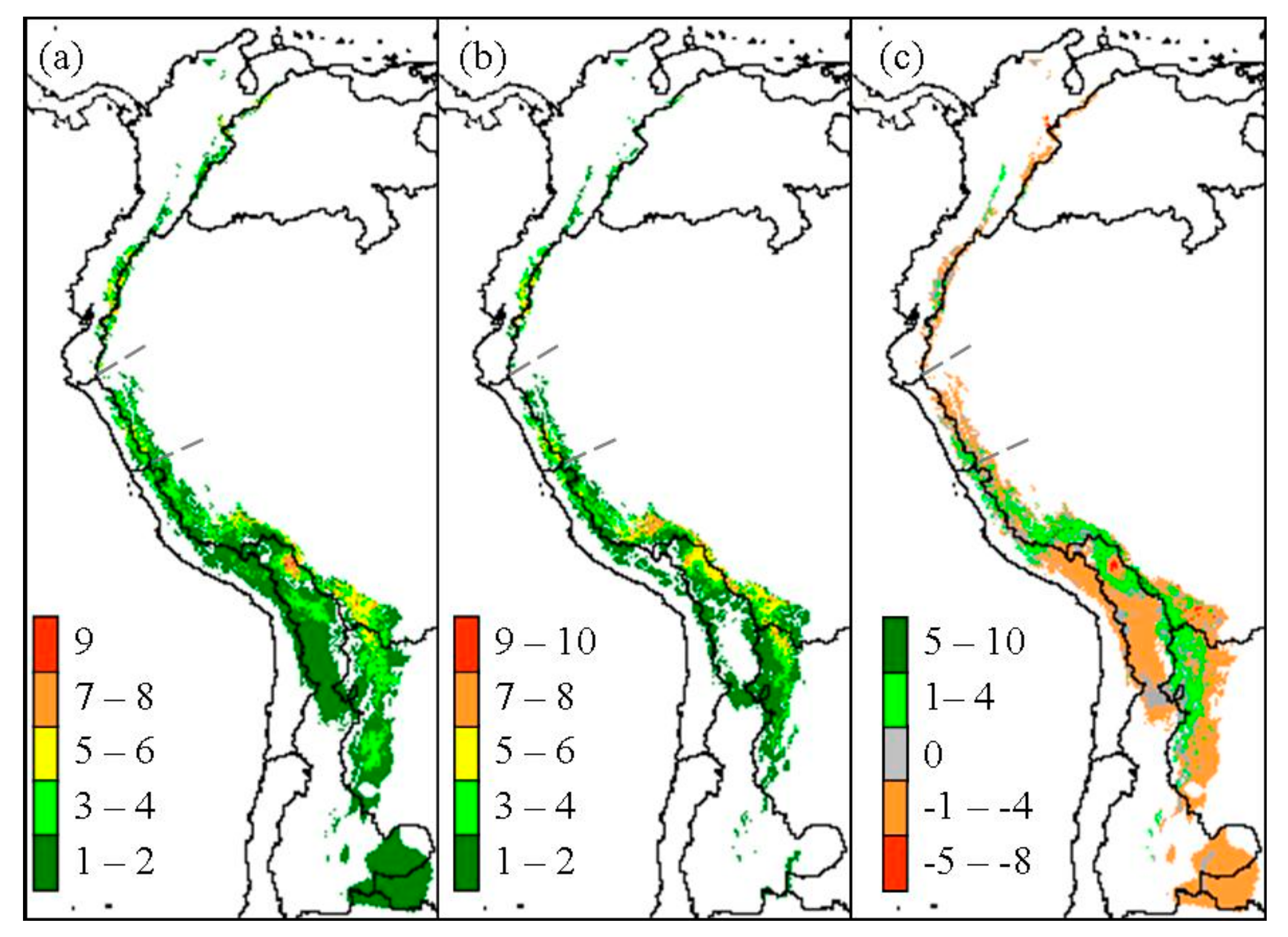
An overall contraction of Polylepis woodland distribution was predicted to have occurred since the LGM based on present climate and CCSM estimations of LGM climate. Overall Polylepis woodland distribution is 36% smaller today than at LGM, with about 249,000 km2 at that time compared to only 158,800 km2 today over its full range from western Venezuela to northern Argentina and Chile. Predicted suitable area for Polylepis species richness along the total length of the Andes reached as many as ten species in a 25 km2 pixel (Figure 1).
The geographic distribution of most Polylepis species was predicted to have contracted or expanded in range by only a small amount since the LGM although in many case by a small amount (Table 1). However two species had major losses in their area of occurrence. P. australis and P. tarapacana are predicted to have contracted to nearly one fourth of their former extent, and the rare P. rugulosa shows a more than a 90% drop in area. These three species are in the south-central Andes near the southern limit of the genus. Mean elevational occurrence increased under present climate conditions by about 1450 m for P. australis and 348 m for P. tarapacana. Polylpeis weberbaueri from Ecuador and northern Peru is predicted to have lost more than half of its LGM area. At the other extreme, two species showed an increase in area of more than 50%. Polylepis besseri distribution in the Altiplano region increased from LGM nearly doubled in predicted area from about 17,180 to31,440 km2. Mean elevation of this species moved upslope by 615 m, with a minimum elevation of 1270 m at LGM to a minimum of 2220 m with present climate Polylepis pepei from southern Peru and Bolivia increased its range by 56% (Table 1).
For the fifteen species with contracting distribution, the mean (± S.E.) stable area of coverage since LGM was 4785 ± 1110 km2 or 20 ± 4% (Table 1). Among the species with the largest contraction in range, P. australis, P. rugulosa, and P. tarapacana from the south-central Andes had among the smallest area predicted to have remained stable to present climate with 4%, 2%, and 0.2% from their maximum extent at LGM, respectively (Table 1). The mean stable area for species with predicted expansion was 3103 ± 289 km2 or 20 ± 2% of their past range. Polylepis besseri, with a large expansion since the LGM, had a stable area of 18% of its predicted extent at LGM.
3.2. Biogeographic Zones
Polylepis species richness per 25 km2 pixel was predicted to decrease within most biogeographic zones since the LGM, except for woodlands in the South Amazon (Table 2, Figure 3). In particular, the North Amazon Basin, which contains significant portions of the northern Andes, was predicted to decrease in the number of Polylepis species within 9960 km2, or about 62% of the total woodland area (Figure 3a). Similarly, a decrease in richness occurred in 67% of the woodlands predicted within the East Jalca Basin. Polylepis species richness was predicted to have remained relatively steady in the West Jalca Basin with areas that increased in richness or remain stable over time to be 93% and 87% of the 1975 km2 extent at LGM, respectively (Figure 3b). The South Amazon Basin was the only biogeographical zone predicted to have greater woodlands area (20,775 km2) with an increase in richness compared to areas that would decrease or remain stable in richness (Figure 3c). This region was predicted to contain the highest number of Polylepis species and pixel areas of increasing richness under both LGM and present climate conditiond. In contrast, the Argentina biogeographic zone was predicted to only contain P. australis at LGM and a mere 325 km2 range would remain today.
Each biogeographic zone was predicted to have changes in Polylepis species richness following changes in mean annual temperature and total annual precipitation (Table 2). As the mean elevation of species rich areas moved upslope in the North and South Amazon zones, areas that lost species had a greater difference between LGM and present annual mean temperature than other areas, with −1.5 and −2.9 °C, respectively. This trend also occurred on the western slopes of the Northwestern Andes. However, both the West and East Jalca zones had the opposite trend with predicted areas of increasing richness possessing a greater difference in mean annual temperature, at or above −2.3 °C, than stable or declining richness areas.
The greatest fractional change in annual precipitation also occurred in predicted areas of increasing richness in the North Amazon, East Jalca, and South Amazon zones, relative to areas of decreasing richness. Species-rich areas today, at higher mean elevations in these zones, tended to be wetter than lower elevation areas that lost Polylepis species richness after the LGM. Only the North Andes and Orinoco zones, at the northern woodland extent in the Andes, and the Paraná, at the southern extent, had either predicted stable or increasing richness in areas currently drier than in the LGM.
Stable areas of species richness tended to have intermediate mean elevation, area, and changes in temperature and precipitation relative to areas with significant changes in species richness. Across the western tropical Andean slopes, in the North Andes, West Jalca and Central Andes biogeographic zones, the mean elevation of stable areas was 3759 m with a mean temperature (± S.E.) of −1.9 ± 0.2 °C. The eastern slope of the tropical Andes, which drains into the Amazon Basin and divided into North Amazon, East Jalca, and South Amazon zones, had similar stable areas with a lower mean elevation of 3688 m and a similar annual mean temperature of −2.0 ± 0.4 °C. Mean fractional change in precipitation indicates drier conditions from LGM to present for both slopes of the tropical Andes with −11.8 ± 6.7% on eastern slopes and −6.8 ± 2.1% on western slopes. The magnitude of climatic change in climatically stable relative to non-stable areas depended on the particular zone. In both the East and West Jalca zones, the mean temperature response was <1 °C and the fractional change in precipitation was no more than 5% in either species richness trend. The Orinoco Basin also had <1 °C mean temperature difference but as much as 24% fractional change in precipitation in stable areas relative to areas with decreasing richness.
4. Discussion
A growing number of paleoecological records have clarified the changing composition and distribution of vegetation belts along the latitudinal length and elevational extent of the Andes during glacial/interglacial episodes. Fossil pollen in the northern Andes suggests that the species-diverse lower vegetation belts moved upslope under warmer interglacial climatic conditions and species-poor high elevation vegetation moved downslope during colder glacial episodes [35]. Portions of the Southern Hemisphere tropical Andes show little fluctuations in plant composition, but contain significant changes in the dominant plant type that would have created plant communities with no modern Andean analogue [22]. Nonetheless, certain vegetation belts such as high elevation páramo grasslands in the northern Andes and puna in the central Andes, and woodlands dominated by Polylepis (Rosaceae) were consistently present throughout Quaternary records [20,36]. Unfortunately, palynological analysis often lack spatial precision since fossil pollen collection sites are often far apart and rely on factors such as wind direction and lake size, resulting in regional rather than local proxies [38]. The identification of Polylepis paleo-woodlands is difficult since fossil pollen is nearly identical to the closely related genus Acaena (Rosaceae) [2]. Although pollen at elevations above 4800 m is more likely to be Polylepis rather than the mostly cloud forest restricted Acaena, paleo-woodlands are often identified as Polylepis/Acaena or Polylepis type [22,38].
The use of species distribution models with climate scenarios for the present and LGM predicted a broad but variable increase in mean elevation of occurrence and contraction of Polylepis woodland distribution since the LGM. Extensive paleoecological records in the central Andes indicate an upslope movement of taxa by more than 1000 m in response to warming since the last glacial period [15]. Polylepis woodlands were predicted to reach their maximum extent during the LGM as colder conditions would have forced them to occupy lower elevations [21] that have greater topographical area.
At high elevations, moraine sites within the Cordillera Blanca of Peru contain remains of Polylepis trees killed by glacial advances up to 400 years BP [39]. Paleoecological evidence suggests climate conditions, including increased wetness and insolation, in the Altiplano 26–14.9 ka may have been beneficial to the expansion of Polylepis populations [21]. Warmer and drier conditions during the Late Pleniglacial (21–14 ka) in the northern Andes widened vegetation belts and upper limits increased in elevation as glaciers retreated [20]. Pollen record provide evidence of the development of Polylepis forests in the southern part of the so-called Andean Depression of southern Ecuador, reflecting warmer and drier climatic conditions during early and mid-Holocene [40].
The range expansion of several Polylepis species in the Altiplano region since LGM reflects the unusual topography of the central Andes. Most predictive models assume range contraction of species distribution with increased elevation following climate warming, since land area typically shrinks with increasing elevation [41]. The topography of the northern and southern Andes follow this pattern, however the central Andes contain the Altiplano, an extensive high-elevation plateau that occurs above 3600 m in elevation in western Bolivia and southern Peru, extending into northern Chile and Argentina. The 250 km-wide plateau will potentially allow more land area following upslope range shift of species in response to climate change [42]. Therefore, previous fluctuations of Polylepis woodlands extent and complex regional topography suggest the potential non-uniform response of species along the length of the Andes following climate change.
The lower limits of Polylepis woodland distribution during and after the LGM are rather unclear. Although fire is expected to be among the most relevant factors limiting the present formation of Polylepis woodland edges at lower elevations [43] the lower elevational limit tends to transition to other forest types [2]. Paleoecological data suggests an approximate lower limit of 1400 m at the time of LGM for Polylepis as the dominant component of upper montane forests in the northern Andes [20]; however our study predicts niche presence at elevations below 1000 m in the Argentina, Altiplano, and Paraná basins at LGM. Nonetheless, these lower elevational niches were predicted to have been lost in the transition to present climate conditions and resulted in decrease in Polylepis species richness in these regions.
On a species level, the magnitude of predicted contraction of distribution range varied by species, with several Polylepis species expanding their range. Fourteen species were predicted to contract their ranges after the LGM, particularly the southernmost limits of P. australis and P. tarapacana and P. rugulosa in the western arid regions. The six species predicted to have expanded their range mostly occur along the southeastern Andes and Altiplano where the central Andean plateau widens to 400 km and an average elevation of 4000 m [44], compared to the narrower 50 km wide and 3000 m elevation sections in Venezuela [45]. In addition, predicted changes in Polylepis species richness is supported by the Quaternary pollen diversity record of species-rich vegetation altitudinal shifts with past climate change [35]. Our study also indicated that climatic changes correlated with shifts in species richness varied by biogeographic zone with marked difference between northern and southern latitudes and east and west slopes of the Andean cordillera. Although precipitation and cold night temperatures may limit Andean vegetation [20], the different predicted changes in mean elevation and species richness highlight the complexity of the Andean topography and climate regimes.
Along with dynamic changes in habitat, the predicted existence and extent of stable areas through Holocene climate fluctuations indicate that conserved areas of woodland continuity served to function as refugia to maintain species richness and narrow endemism. Major refugial areas were predicted to occur in the eastern Andean slopes of the southern Amazon Basin, Altiplano, and Paraná. The predicted lower limit of refugia, near 2000 m in elevation for most of the tropical Andes, coincides with paleoecological data indicating the lower limits of the Polylepis vegetation belt from the LGM to present in the northern Andes [20]. However, the extent of the refugial belt was predicted to vary by biogeographic zone and far lower limits were predicted to occur in the Altiplano and southern ranges of the Andes.
Although Quaternary records indicate the widespread occurrence of Polylepis woodlands [21], other studies have proposed that Polylepis woodlands did not form permanent continuous woodlands before human arrival [9]. The predicted stable areas in this study suggest the existence of conserved Polylepis species niches with climate change and the potential for continuous woodland associations in regions of high Polylepis species richness. The aggregated pattern of Polylepis-specialist birds in the Cordillera Blanca and Cusco region of Peru suggests isolation from other forest types during Pleistocene glacial periods [5]. These stable areas also indicate key refugial zones for many associated endemic species following climate change and may help understand the mechanisms underlying local endemism and genetic diversity of flora and fauna [46]. These regions appear to support multiple core species populations, which include a variety of Polylepis-associated bird and mammal species, including the pampas cat (Leopardus colocolo) [7,47].
The use of bioclimatic models and SDM algorithms comes with many significant advantages and inherent limits that should be addressed to properly put predictive models into context. Generally, climatic models based on historic climate station data are required to extrapolate in time and space due to the lack of continuous data in various locations causing significant gaps in information [23]. The confidence in these temperature data are reasonable due to the relationship between elevation and temperature, but precipitation numbers are often questioned in mountainous regions due to the low density of climate stations [23]. Therefore, caution must be taken on how distribution models are constructed and interpreted. Nonetheless bioclimatic models, as the model used in this study, can provide a useful approximation of species response to changes in climate using the central biogeographic premise that climate has a dominant control over the natural distribution of a species [48,49]. Biotic interactions, a species’ dispersal ability, genetic variation, and anthropogenic activity are major factors to species distribution that are not incorporated directly in SDM frameworks and have been repeatedly criticized due to this inherent limitation [50,51].
Indeed, much of Polylepis current distribution may reflect extensive anthropogenic pressures resulting in fragmented populations in different regions, reduced quantity of geographic point localities and an altered realized niche. The debate includes if the present fragmentation largely occurred before or after Spanish colonization of the region and if the current location of populations reflect land use rather than natural environmental extent. Regardless, the representativeness of the current distribution directly affects present and past modeling with the potential of under estimating distribution in both scenarios. We find a few models of our study to have disjunctive potential habitats, which would be difficult to support but are a result of these distant and isolated populations (Table 1). Nevertheless, the use of a representative sample size or a diverse set of point localities should provide enough information to achieve a statistically robust prediction a species’ geographic range through spatial modeling. It is also notable to address issues in species identification, since isolated Polylepis species populations have been recorded far from any neighboring populations. As with many taxa, there are uncertainty in present species identification and taxonomic concepts and the Polylepis genus is no exception. There has been extensive hybridization in various landscapes, including from intentional introductions [52]. Care must be taken in including the most reasonable point locations from digital taxonomic databases and those made available by local experts.
One final characteristic of SDMs worth discussing is the spatial resolution of the environmental layers and models. The spatial resolution of present and past climate variables at 25 km2 does not capture all the variation that can occur within this pixel area. Andean topography is complex and fine-scale distribution patterns of Polylepis woodlands can be confined to slopes and habitats defined by microclimates and land use pressures, which would not be accurately represented within the pixel. This limits our approach to answer the larger question of the fate of these woodlands after civilizations established themselves in the Andes. Although the lack of detailed resolution is a common limitation of geospatial modeling, our objective was to identify the fluctuations in suitable areas across the region. The large scale patterns across the biogeographic basins can tell us more on distribution patterns and limitations than small-scale patterns associated with local conditions.
SDMs have the potential to increase our understanding species response to past climate fluctuations and therefore understanding future distribution dynamics with anthropogenic climate change. Paleoecological data has provided key insights into the extent of Polylepis woodlands, but without species level identification as we have shown, the generalized response of Polylepis species distribution to temperature and precipitation will remain unclear. SDMs can provide a spatial perspective on species response and species richness that is directly applicable to current conservation efforts to preserve Polylepis woodlands. Temporally stable areas, as a refuge for many Polylepis associated species, will be key factor for conservation during anthropogenic climate forcing since their protection and management may reflect the persistence of Polylepis woodlands in the future.
5. Conclusions
The fragmented distribution of Polylepis woodlands present important questions regarding past response of high Andean vegetation to climate change. Although paleoeclimatic records from the Quaternary indicate that major fluctuations in elevational changes in climate have occurred, the absence of species level paleoecological data have limited our understanding of Polylepis species response to changes in glacial extent and climate. Hindcasting presents an approach to predict refugial areas and the extent of contraction and expansion of Polylepis species woodlands since the LGM, and thereby stable areas of species endemism and high species richness in the high-elevation Andes. The extent of Polylepis woodland today is 36% smaller today than at LGM, however, a few species have experienced a projected increase in range of 180%. Much of those changes have occurred at the interface of the southern Amazonian Basin with the Altiplano where Polylepis species richness is highest. Bioclimatically stable areas for each species from the LGM to the present averaged 20 ± 4% of the modeled range and mostly occurred in disjunct pockets from central Peru to northern Argentina and Chile. Polylepis woodlands with their high number of endemic species are keystone habitats for biodiversity in an often treeless alpine landscape and may have played a similar function in the past.
Supplementary Materials
The following are available online at www.mdpi.com/1999-4907/8/7/232/s1, Figure S1: Potential present species distribution for each Polylepis species in this study, Table S1: Geographic location and source information for the presence data of 21 species of Polylepis, Table S2: Relative contributions (%) of environmental variables to Maxent models for Polylepis species, Table S3: Means of proportional predicted area (Area) and test omission rates (OR) at the 10% cumulative threshold, area under the receiver operating characteristic curve (AUC) and test gains for all models of Polylepis species.
Acknowledgments
This research was funded by a grant from the University of California Pacific Rim Program, a Stephen A. Vavra Fund Research Grant, and a UCLA Latin America Center Grant (to B.R.Z.). We would also like to thank Guillermo Velazco for help with field collection in Peru, Fundación ProYungas of Argentina and the late Clodomiro Marticorena from Universidad de Concepción, Chile for providing additional data on Polylepis distributions.
Author Contributions
B.R.Z. and P.W.R. conceived of the project and designed the analytical approach. Both B.R.Z. and P.W.R. contributed data used in the analyses, and B.R.Z. carried out the modeling effort. Both authors shared in the writing and editing of the manuscript.
Conflicts of Interest
The authors declare no conflict of interest, and have no personal circumstances or interest that may be perceived as inappropriately influencing the representation or interpretation of reported research results. The founding sponsors had no role in the design of the study; in the collection, analyses, or interpretation of data; in the writing of the manuscript, and in the decision to publish the results.
References
- Simpson, B.B. A revision of the genus Polylepis (Rosaceae: Sanguisorbeae). Smithson. Contrib. Bot. 1979, 43, 1–62. [Google Scholar] [CrossRef]
- Kessler, M. The “Polylepis Problem”: Where do we stand? Ecotropica 2002, 8, 97–110. [Google Scholar]
- Purcell, J.; Brelsford, A.; Kessler, M. The world’s highest forest: A better understanding of the properties of Andean queñua woodlands has major implications for their conservation. Am. Sci. 2004, 92, 454–461. [Google Scholar] [CrossRef]
- The IUCN Red List of Threatened Species. Available online: www.iucnredlist.org (accessed on 7 March 2017).
- Fjeldså, J. Polylepis forests—Vestiges of a vanishing ecosystem in the Andes. Ecotropica 2002, 8, 111–123. [Google Scholar]
- Aucca, C.; Ramsay, P.M. Management of biodiversity and land use in southern Peru: ECOAN’s activities to help conserve Polylepis woodlands. Mt. Res. Dev. 2005, 25, 287–289. [Google Scholar] [CrossRef]
- Ellenberg, H. Wald oder Steppe? Die natürliche Pflanzendecke der Anden Perus (I, II). Umschau Wissen. Technol. 1958, 21, 645–648, 22, 679–681. [Google Scholar]
- Simpson, B.B. Speciation and Specialization of Polylepis in the Andes. High Altitude Tropical Biogeography; Vulllemeire, F., Monasterio, M., Eds.; Oxford University Press: Oxford, UK, 1986; pp. 304–316. [Google Scholar]
- Gosling, W.D.; Hanselman, J.A.; Knox, C.; Valencia, B.G.; Bush, M.B. Long-term drivers of change in Polylepis woodland distribution in the central Andes. J. Veg. Sci. 2009, 20, 1041–1052. [Google Scholar] [CrossRef]
- Toivonen, J.M.; Horna, V.; Kessler, M.; Ruokolainen, K.; Hertel, D. Interspecific variation in functional traits in relation to species climatic niche optima in Andean Polylepis (Rosaceae) tree species: Evidence for climatic adaptations. Funct. Plant Biol. 2014, 41, 301–312. [Google Scholar] [CrossRef]
- Gosling, W.D.; Bunting, M.J. A role of palaeoecology in anticipating future change in mountain regions? Palaeogeogr. Palaeoclimatol. Palaeoecol. 2008, 259, 1–5. [Google Scholar] [CrossRef]
- MacDonald, G.M.; Bennett, K.D.; Jackson, S.T.; Parducci, L.; Smith, F.A.; Smol, J.P.; Willis, K.J. Impacts of climate change on species, populations and communities: Palaeobiogeographical insights and frontiers. Prog. Phys Geogr. 2008, 32, 139–172. [Google Scholar] [CrossRef]
- Clark, P.U.; Dyke, A.S.; Shakun, J.D.; Carlson, A.E.; Clark, J.; Wohlfarth, B.; Mitrovica, J.X.; Hostetler, S.W.; McCabe, A.M. The last glacial maximum. Science 2009, 325, 710–714. [Google Scholar] [CrossRef] [PubMed]
- Smith, J.A.; Seltzer, G.O.; Farber, D.L.; Rodell, D.T.; Finkel, R.C. Early local last glacial maximum in the tropical Andes. Science 2005, 308, 678–681. [Google Scholar] [CrossRef] [PubMed]
- Bush, M.B.; Silman, M.R.; Urrego, D.H. 48,000 years of climate and forest change in a biodiversity hot spot. Science 2004, 303, 827–829. [Google Scholar] [CrossRef] [PubMed]
- Urrego, D.H.; Bush, M.B.; Silamn, M.R.; Correa-Metrio, A.; Ledru, M.-P.; Mayle, F.E.; Paduano, G.; Valencia, B.G. Millennial-scale ecological changes in tropical South America since the last glacial maximum. In Past Climate Variability in South America and Surrounding, Developments in Paleoenvironmental Research 14; Vimeux, F., Ed.; Springer: New York, NY, USA, 2009; pp. 283–300. [Google Scholar]
- Carnaval, A.C.; Moritz, C. Historical climate modelling predicts patterns of current biodiversity in the Brazilian Atlantic forest. J. Biogeogr. 2008, 35, 1187–1201. [Google Scholar] [CrossRef]
- Nogués-Bravo, D. Predicting the past distribution of species climatic niches. Glob. Ecol. Biogeogr. 2009, 18, 521–531. [Google Scholar] [CrossRef]
- Rodríguez-Sánchez, F.; Arroyo, J. Reconstructing the demise of Tethyan plants: Climate-driven range dynamics of Laurus since the Pliocene. Glob. Ecol. Biogeogr. 2008, 17, 685–695. [Google Scholar] [CrossRef]
- Hooghiemstra, H.; van der Hammen, T. Quaternary Ice-Age dynamics in the Colombian Andes: Developing an understanding of our legacy. Philos. Trans. R. Soc. B 2004, 359, 173–181. [Google Scholar] [CrossRef] [PubMed]
- Chepstow-Lusty, A.; Bush, M.B.; Frogley, M.R.; Baker, P.A.; Fritz, S.C.; Aronson, J. Vegetation and climate change on the Bolivian Altiplano between 108,000 and 18,000 yr ago. Quat. Res. 2005, 63, 90–98. [Google Scholar] [CrossRef]
- Gosling, W.D.; Bush, M.B.; Hanselman, J.A.; Chepstow-Lusty, A. Glacial-interglacial changes in moisture balance and the impact on vegetation in the southern hemisphere tropical Andes (Bolivia/Peru). Palaeogeogr. Palaeoclimatol. Palaeoecol. 2008, 259, 35–50. [Google Scholar] [CrossRef]
- Hijmans, R.J.; Cameron, S.E.; Parra, J.L.; Jones, P.G.; Jarvis, A. Very high resolution interpolated climate surfaces for global land areas. Int. J. Climatol. 2005, 25, 1965–1978. [Google Scholar] [CrossRef]
- Otto-Bliesner, B.L.; Brady, E.C.; Clauzet, G.; Tomas, R.; Levis, S.; Kothavala, Z. Last Glacial Maximum and Holocene climate in CCSM3. J. Clim. 2006, 19, 2526–2544. [Google Scholar] [CrossRef]
- Braconnot, P.; Otto-Bliesner, B.; Harrison, S.; Joussaume, S.; Peterchmitt, J.-Y.; Abe-Ouchi, A.; Crucifix, M.; Driesschaert, E.; Fichefet, T.; Hewitt, C.D.; et al. Results of PMIP2 coupled simulations of the Mid-Holocene and Last Glacial Maximum—Part 1: Experiments and large-scale features. Clim. Past 2007, 3, 261–277. [Google Scholar] [CrossRef]
- Phillips, S.; Anderson, R.P.; Schapire, R.E. Maximum entropy modelling of species geographic distributions. Ecol. Model. 2006, 190, 231–259. [Google Scholar] [CrossRef]
- Wisz, M.S.; Hijmans, R.J.; Li, J.; Peterson, A.T.; Graham, C.H.; Guisan, A. Effects of sample size on the performance of species distribution models. Divers. Distrib. 2008, 14, 763–773. [Google Scholar] [CrossRef]
- Phillips, S.; Dudík, M. Modeling of species distributions with Maxent: New extensions and a comprehensive evaluation. Ecography 2008, 31, 161–175. [Google Scholar] [CrossRef]
- Csuti, B. Mapping animal distribution areas for gap analysis. In Gap Analysis: A Landscape Approach to Biodiversity Planning; Scott, J.M., Tear, T.H., Davis, F.W., Eds.; American Society for Photogrammetry and Remote Sensing: Bethesda, MD, USA, 1996; pp. 135–145. [Google Scholar]
- Hurlbert, A.P.; Jetz, W. Species richness, hotspots, and the scale-dependence of range maps in ecology and conservation. Proc. Natl. Acad. Sci. USA 2007, 104, 13384–13389. [Google Scholar] [CrossRef] [PubMed]
- Loarie, S.R.; Carter, B.E.; Hayhoe, K.; McMahon, S.; Moe, R.; Knight, C.A.; Ackerly, D.D. Climate change and the future of California’s endemic flora. PLoS ONE 2008, 3, e2502. [Google Scholar] [CrossRef] [PubMed]
- Phillips, S. A brief Tutorial on Maxent; ATandT Research: Florham Park, NJ, USA, 2005; Available online: http://www.cs.princeton.edu/_schapire/maxent/tutorial/tutorial.doc (accessed on 7 March 2017).
- Buermann, W.; Saatchi, S.; Smith, T.B.; Zutta, B.R.; Chaves, J.A.; Milá, B.; Graham, C.H. Predicting species distribution across the Amazonian and Andean regions using remote sensing data. J. Biogeogr. 2008, 35, 1160–1176. [Google Scholar] [CrossRef]
- Riordan, E.C.; Rundel, P.W. Modelling the distribution of a threatened habitat: The California sage scrub. J. Biogeogr. 2009, 36, 2176–2188. [Google Scholar] [CrossRef]
- US Geological Survey (USGS). HYDRO1K Elevation Derivative Database; Earth Resources Observation and Science (EROS) Data Center (EDC): Sioux Falls, SD, USA, 1996. Available online: http://edc.usgs.gov/products/elevation/gtopo30/hydro/index.html (accessed on 7 March 2017).
- Luteyn, J.L. Páramos: A Checklist of Plant Diversity, Geographical Distribution, and Botanical Literature; New York Botanical Garden Press: New York, NY, USA, 1999. [Google Scholar]
- Weigend, M. Observations on the biogeography of the Amotape-Huancabamba zone in northern Peru. Bot. Rev. 2002, 68, 38–54. [Google Scholar] [CrossRef]
- Weng, C.; Hooghiemstra, H.; Duivenvoorden, J.F. Response of pollen diversity to the climate-driven altitudinal shift of vegetation in the Colombian Andes. Philos. Trans. R. Soc. B 2007, 362, 253–262. [Google Scholar] [CrossRef] [PubMed]
- Jomelli, V.; Favier, V.; Rabatel, A.; Brunstein, D.; Hoffman, G.; Francou, B. Fluctuations of glaciers in the tropical Andes over the last millennium and paleoclimatic implications: A review. Palaeogeogr. Palaeoclimatol. Palaeoecol. 2009, 281, 269–282. [Google Scholar] [CrossRef]
- Rodríguez, F.; Behling, H. Late Quaternary vegetation, climate and fire dynamics, and evidence of early to mid-Holocene Polylepis forests in the Jimbura region of the southernmost Ecuadorian Andes. Palaeogeogr. Palaeoclimatol. Palaeoecol. 2012, 350, 247–257. [Google Scholar] [CrossRef]
- Colwell, R.K.; Brehm, G.; Cardelús, C.L.; Gilman, A.C.; Longino, J.T. Global warming, elevational range shifts, and lowland biotic attrition in the wet tropics. Science 2008, 10, 258–261. [Google Scholar] [CrossRef] [PubMed]
- Elsen, P.R.; Tingley, M.W. Global mountain topography and the fate of montane species under climate change. Nat. Clim. Chang. 2015, 5, 772–776. [Google Scholar] [CrossRef]
- Cierjacks, A.; Wesche, K.; Hensen, I. Potential lateral expansion of Polylepis forest fragments in central Ecuador. For. Ecol. Manag. 2007, 242, 477–486. [Google Scholar] [CrossRef]
- Garzione, C.N.; Hoke, G.D.; Libarkin, J.C.; Withers, S.; MacFadden, B.; Eiler, J.; Ghosh, P.; Mulch, A. Rise of the Andes. Science 2008, 6, 1304–1307. [Google Scholar] [CrossRef] [PubMed]
- Cuatrecasas, J. Speciation and radiation of the Espeletiinae in the Andes. In High. Altitude Tropical Biogeography; Vuilleumier, F., Monasterio, M., Eds.; Oxford University Press: New York, NY, USA, 1986; pp. 267–303. [Google Scholar]
- Carnaval, A.C.; Hickerson, M.J.; Haddad, C.F.B.; Rodrigues, M.T.; Moritz, C. Stability predicts genetic diversity in the Brazilian Atlantic forest hotspot. Science 2009, 303, 785–789. [Google Scholar] [CrossRef] [PubMed]
- Cossios, D.; Lucherini, M.; Ruiz-García, M.; Angers, B. Influence of ancientglacial periods on the Andean fauna: the case of the pampas cat (Leopardus colocolo). BMC Evol. Biol. 2009, 9. [Google Scholar] [CrossRef] [PubMed]
- Pearson, R.G.; Dawson, T.P. Predicting the impacts of climate change on the distribution of species: Are bioclimate envelope models useful? Glob. Ecol. Biogeogr. 2003, 12, 361–371. [Google Scholar] [CrossRef]
- Beaumont, L.J.; Hughes, L.; Poulsen, M. Predicting species distributions: Use of climatic parameters in BIOCLIM and its impact on predictions of species’ current and future distributions. Ecol. Model. 2005, 186, 250–269. [Google Scholar] [CrossRef]
- Hampe, A. Bioclimatic envelope models: What they detect and what they hide. Glob. Ecol. Biogeogr. 2004, 13, 469–471. [Google Scholar] [CrossRef]
- Pearson, R.G.; Dawson, T.P. Bioclimatic envelope models: What they detect and what they hide—Response to Hampe. Glob. Ecol. Biogeogr. 2004, 13, 471–473. [Google Scholar] [CrossRef]
- Kessler, M.; Schmidt-Lebuhn, A.N. Taxonomical and distributional notes on Polylepis (Rosaceae). Org. Divers. Evol. 2006, 6, 67–69. [Google Scholar] [CrossRef]
Figure 1.
Past (a), present (b), and overall change (c) of Polylepis species richness predicted with Community Climate System Model (CCSM) global circulation model. Overlaying the ≥50% probability of each species predicted distribution was used to estimate richness.
Figure 1.
Past (a), present (b), and overall change (c) of Polylepis species richness predicted with Community Climate System Model (CCSM) global circulation model. Overlaying the ≥50% probability of each species predicted distribution was used to estimate richness.

Figure 2.
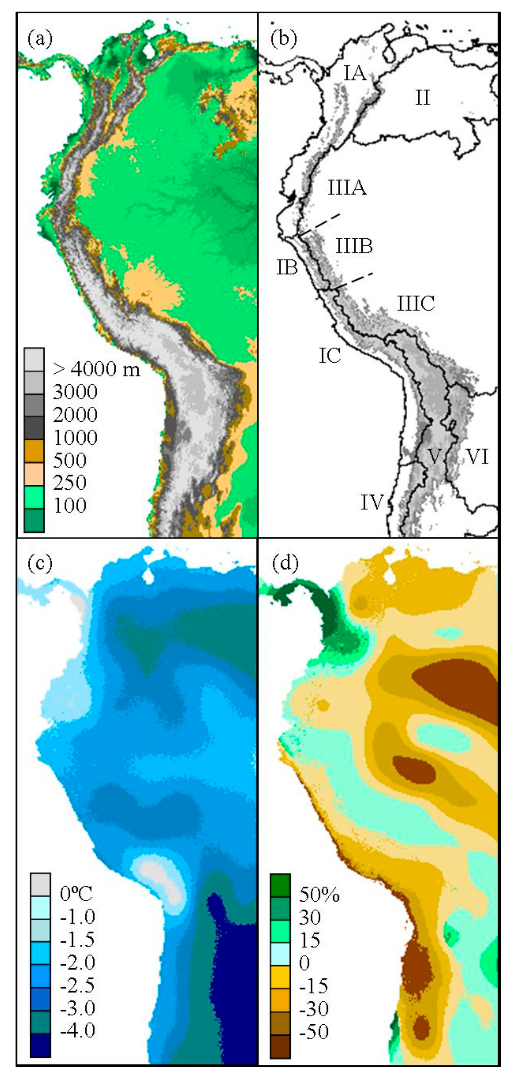
(a) Present elevation and (b) hydrological basins and subdivisions of the tropical and subtropical Andean cordillera. The San Juan Basin is divided into the subdivisions of North Andes (IA), West Jalca (IB), Central Andes (IC), and the Orinoco Basin (II). The Amazon Basin is divided into the subdivisions of North Amazon (IIIA), East Jalca (IIIB), and South Amazon (IIIC). The southern basins include Argentina (IV), Altiplano (V), and Paraná (VI). Present elevation greater or equal to 1000 m is indicated in gray scale. The annual mean temperature difference (c) and fractional change in precipitation (d) from present is given using CCSM simulation of LGM climate.
Figure 2.
(a) Present elevation and (b) hydrological basins and subdivisions of the tropical and subtropical Andean cordillera. The San Juan Basin is divided into the subdivisions of North Andes (IA), West Jalca (IB), Central Andes (IC), and the Orinoco Basin (II). The Amazon Basin is divided into the subdivisions of North Amazon (IIIA), East Jalca (IIIB), and South Amazon (IIIC). The southern basins include Argentina (IV), Altiplano (V), and Paraná (VI). Present elevation greater or equal to 1000 m is indicated in gray scale. The annual mean temperature difference (c) and fractional change in precipitation (d) from present is given using CCSM simulation of LGM climate.

Figure 3.
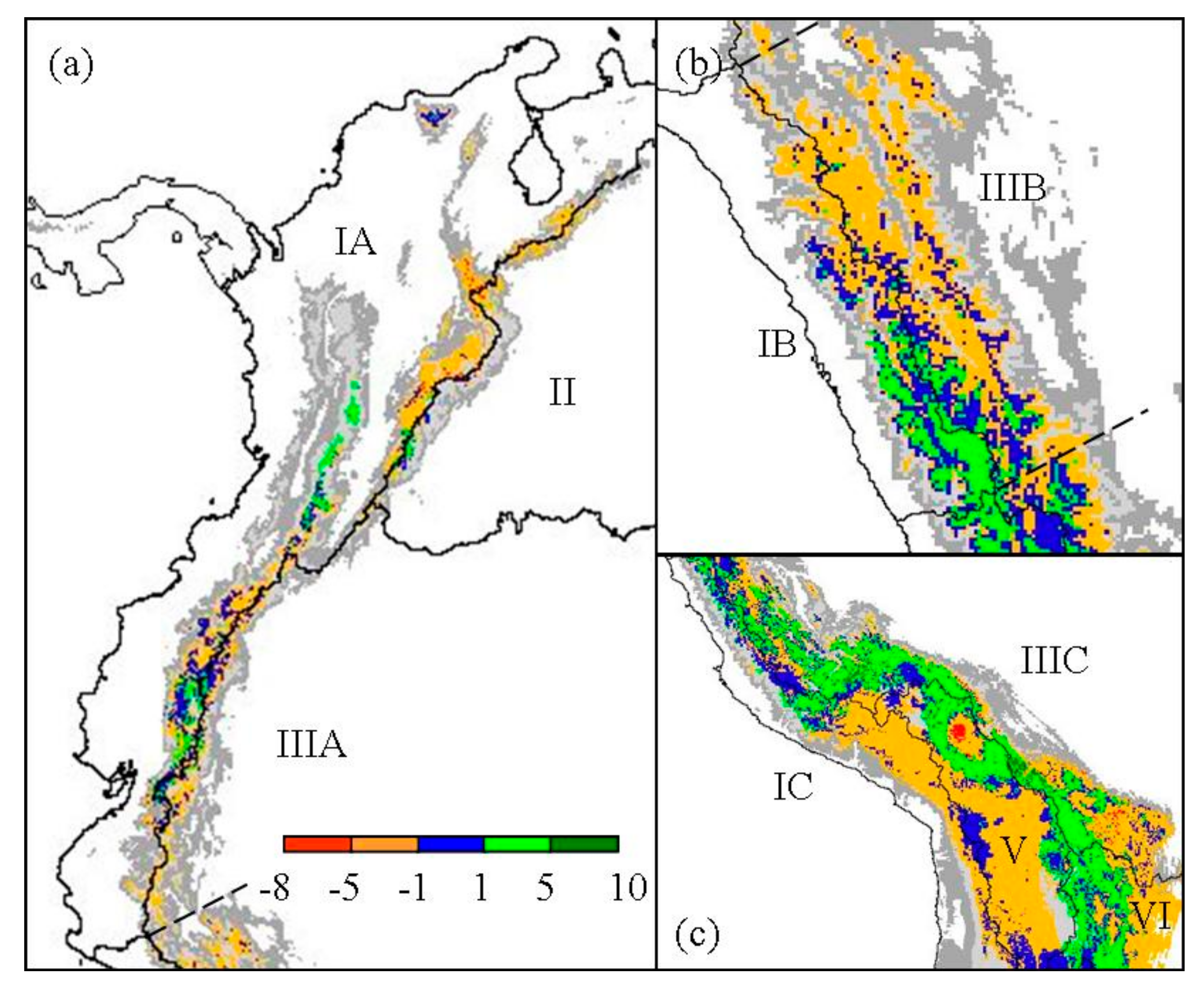
Regional change of Polylepis species richness for (a) North Andes (IA), Orinoco (II), and North Amazon (IIIA); (b) West and East Jalca (IB, IIIB); and (c) the southern zones of Central Andes (IC), South Amazon (IIIC), Altiplano (V), and Paraná (VI). Refugial areas are highlighted in blue. Present elevation greater or equal to 1000 m is indicated in gray scale.
Figure 3.
Regional change of Polylepis species richness for (a) North Andes (IA), Orinoco (II), and North Amazon (IIIA); (b) West and East Jalca (IB, IIIB); and (c) the southern zones of Central Andes (IC), South Amazon (IIIC), Altiplano (V), and Paraná (VI). Refugial areas are highlighted in blue. Present elevation greater or equal to 1000 m is indicated in gray scale.


Table 1.
Area and middle elevation of Polylepis species distribution predicted with the CCSM global circulation model of past climate and Worldclim present climate model.
Table 1.
Area and middle elevation of Polylepis species distribution predicted with the CCSM global circulation model of past climate and Worldclim present climate model.
| Species | Site | Range | Hydrologic Basin | Predicted Area (km2) | Middle Elevation (m) | ||||
|---|---|---|---|---|---|---|---|---|---|
| Past | Present | Stable | Past | Present | Change of Middle | ||||
| P. australis | 61 | Central and north-western Argentina (e) | Mostly VI and some neighboring areas of the V and IV basins | 63,460 | 12,450 | 2290 | 809 (52–3732) | 2263 (805–3951) | +1454 |
| P. besseri | 80 | Southern Peru to Bolivia | VI, eastern V, southern Amazon and San Juan basins | 17,185 | 31,445 | 3130 | 3142 (1276–4334) | 3757 (2216–4892) | +615 |
| P. crista-galli | 33 | Southern Bolivia to northernmost Argentina | Mostly VI and some neighboring areas of IIIC | 18,225 | 16,520 | 1590 | 2048 (337–3883) | 2963 (1264–4024) | +915 |
| P. hieronymi | 41 | Southern Bolivia to northern Argentina | VI and sIIIC | 23,850 | 12,645 | 1490 | 1299 (292–3026) | 2153 (926–3563) | +854 |
| P. incana | 115 | Ecuador to southern Peru | Western and southern Amazon, northern and central San Juan basins | 25,885 | 22,485 | 8160 | 3736 (559–4908) | 4001 (1588–5035) | +265 |
| P. incarum | 57 | Southern Peru to Bolivia | Southern Amazon and V basins | 18,075 | 28,310 | 3235 | 3586 (1162–5037) | 4076 (1591–5243) | +490 |
| P. lanata | 40 | Southern Peru to Bolivia | IIIC | 19,690 | 15,525 | 4160 | 3443 (1771–4525) | 3628 (1693–4775) | +185 |
| P. lanuginosa | 20 | Ecuador (e) | Northwest San Juan and northwest Amazon basins | 6165 | 6125 | 600 | 3112 (1673–4728) | 3342 (2234–5280) | +230 |
| P. neglecta | 32 | Central and southern Bolivia (e) | Mostly IIIC and some neighboring areas of VI basin | 13,315 | 15,035 | 2465 | 2327 (1056–3634) | 2883 (1273–4049) | +556 |
| P. pacensis | 20 | Western Bolivia (e) | Mostly IIIC and some neighboring areas of V | 17,085 | 20,385 | 3680 | 3564 (1492–5057) | 3847 (1425–5407) | +283 |
| P. pauta | 42 | Ecuador and isolated populations in southeastern Peru and northern Bolivian Andes | Northern San Juan, neighboring areas of the northwestern Amazon Basin and isolated areas of the IIIC | 23,375 | 16,690 | 5590 | 3141 (1366–4908) | 3449 (1569–5280) | +308 |
| P. pepei | 30 | Central Peru to northeastern Bolivia | IIIC | 12,890 | 16,215 | 3990 | 3843 (1614–5130) | 3984 (1631–5585) | +141 |
| P. racemosa | 56 | Northern Peru to northwestern Bolivia, isolated population in Ecuador | Northern San Juan to IIIC | 30,300 | 29,945 | 7745 | 3577 (1495–4600) | 3873 (1759–5236) | +296 |
| P. reticulata | 34 | Ecuador and isolated populations in northern and central Peru | Northern to central San Juan basin | 7300 | 5890 | 3555 | 3516 (2564–5280) | 3613 (2927–5280) | +97 |
| P. rugulosa | 24 | Southwestern Peru to northernmost Chile | Central San Juan to western V | 38,495 | 8840 | 745 | 4034 (1340–5804) | 4063 (1811–5498) | +29 |
| P. sericea | 90 | Venezuela to Bolivia | Northern San Juan to IIIC | 36,455 | 35,740 | 15,010 | 3708 (1202–5280) | 3957 (1613–5280) | +249 |
| P. subtusalbida | 92 | Central Bolivia (e) | IIIC | 15,485 | 19,415 | 2120 | 3155 (1927–4305) | 3645 (1932–4608) | +490 |
| P. tarapacana | 62 | Border regions of Argentina, Bolivia, Chile, and Peru | V and VI | 52,145 | 13,515 | 85 | 4168 (2224–5804) | 4517 (2749–5498) | +349 |
| P. tomentella | 122 | Southern Bolivia to northwestern Argentina with isolated populations in central Peru | Central San Juan, V, IIIC and VI | 40,515 | 35,630 | 4940 | 3315 (930–4568) | 3635 (1720–4670) | +320 |
| P. triacontandra | 61 | Southern Peru to Bolivia, with few isolated populations in central Peru | Mostly IIIC and some neighboring areas of the V. Isolated areas in the central San Juan basin | 22,740 | 21,190 | 11,690 | 4177 (2835–5563) | 4222 (1955–5585) | +45 |
| P. weberbaueri | 82 | Ecuador to southern Peru | Northen San Juan to IIIC | 26,745 | 13,535 | 4130 | 3924 (1437–5280) | 3990 (1776–5280) | +66 |
Area predicted to be stable are pixels with no change in presence from past to present climate. Predicted ranges of elevation for each scenario are shown in parenthesis. Endemic species (e) are noted with range.
Table 2.
Changes in predicted Polylepis species richness per 25 km2 pixel since Last Glacial Maximum (LGM) within basins and biogeographic zones of tropical and subtropical Andes.
Table 2.
Changes in predicted Polylepis species richness per 25 km2 pixel since Last Glacial Maximum (LGM) within basins and biogeographic zones of tropical and subtropical Andes.
| Basin | Biogeo. Zone | Species Richness Response | Area (km2) | Mean Elevation (m) | Temp from Present (°C) | Prec. from Present (%) |
|---|---|---|---|---|---|---|
| San Juan | IA | Decrease | 9960 | 2458 (559–4335) | −4.1 | |
| Stable | 3760 | 3450 (1997–4834) | −1.5 | −1.1 | ||
| Increase | 2320 | 3499 (2251–5280) | −1.8 | 15.0 | ||
| IB | Decrease | 1975 | 3258 (2154–5563) | −2.0 | −5.6 | |
| Stable | 1710 | 3733 (2752–5229) | −2.2 | −10.2 | ||
| Increase | 1840 | 4341 (2294–5243) | −2.3 | −10.1 | ||
| IC | Decrease | 16,870 | 3869 (1340–5804) | −1.2 | −29.3 | |
| Stable | 6760 | 4094 (2233–5347) | −1.9 | −24.1 | ||
| Increase | 4060 | 4154 (1972–4921) | −2.1 | −19.4 | ||
| Orinoco | II | Decrease | 1815 | 2797 (1673–4024) | −2.6 | −12.1 |
| Stable | 285 | 3352 (2838–3923) | −2.8 | 12.4 | ||
| Increase | 270 | 3604 (2698–4110) | −2.8 | 24.3 | ||
| Amazon | IIIA | Decrease | 2975 | 2996 (2085–4183) | −1.5 | −1.8 |
| Stable | 1335 | 3481 (2613–4908) | −1.3 | −5.5 | ||
| Increase | 450 | 3663 (2640–5035) | −1.3 | −4.7 | ||
| IIIB | Decrease | 7030 | 3275 (2132–4348) | −2.1 | −2.3 | |
| Stable | 2580 | 3787 (2669–5119) | −2.3 | −4.0 | ||
| Increase | 850 | 4233 (3336–5219) | −2.4 | −5.2 | ||
| IIIC | Decrease | 20,745 | 2939 (1056–5053) | −2.9 | −8.5 | |
| Stable | 10,595 | 3795 (1605–5374) | −2.4 | −10.8 | ||
| Increase | 20,775 | 4026 (1758–5585) | −2.4 | −11.7 | ||
| Argentina | IV | Decrease | 3420 | 602 (121–1148) | −3.9 | 8.7 |
| Stable | 325 | 1401 (1053–1978) | −3.6 | 6.7 | ||
| Increase | - | - | - | - | ||
| Altiplano | V | Decrease | 47,680 | 2761 (152–5476) | −2.2 | −16.2 |
| Stable | 15,755 | 3854 (805–5498) | −2.7 | −16.5 | ||
| Increase | 11,640 | 4000 (1867–5195) | −2.8 | −12.7 | ||
| Paraná | VI | Decrease | 39,900 | 924 (92–4901) | −4.3 | 5.3 |
| Stable | 10,010 | 3006 (106–5930) | −4.0 | 1.7 | ||
| Increase | 15,865 | 3539 (1380–5161) | −4.0 | 5.5 |
See methods for the calculation of mean temperature and precipitation changes from present at LGM. Predicted ranges of elevation are shown in parenthesis.
© 2017 by the authors. Licensee MDPI, Basel, Switzerland. This article is an open access article distributed under the terms and conditions of the Creative Commons Attribution (CC BY) license (http://creativecommons.org/licenses/by/4.0/).
Share and Cite
MDPI and ACS Style
Zutta, B.R.; Rundel, P.W. Modeled Shifts in Polylepis Species Ranges in the Andes from the Last Glacial Maximum to the Present. Forests 2017, 8, 232. https://doi.org/10.3390/f8070232
AMA Style
Zutta BR, Rundel PW. Modeled Shifts in Polylepis Species Ranges in the Andes from the Last Glacial Maximum to the Present. Forests. 2017; 8(7):232. https://doi.org/10.3390/f8070232
Chicago/Turabian StyleZutta, Brian R., and Philip W. Rundel. 2017. "Modeled Shifts in Polylepis Species Ranges in the Andes from the Last Glacial Maximum to the Present" Forests 8, no. 7: 232. https://doi.org/10.3390/f8070232
Note that from the first issue of 2016, this journal uses article numbers instead of page numbers. See further details here.