Automatic Mapping of Forest Stands Based on Three-Dimensional Point Clouds Derived from Terrestrial Laser-Scanning


1
Department of Forest- and Soil Science, Institute of Forest Growth, University of Natural Resources and Life Sciences (BOKU), Vienna 1180, Austria
2
Department of Landscape, Spatial and Infrastructure Sciences, Institute of Applied Statistics and Computing, University of Natural Resources and Life Sciences (BOKU), Vienna 1180, Austria
*
Author to whom correspondence should be addressed.
Forests 2017, 8(8), 265; https://doi.org/10.3390/f8080265
Submission received: 6 July 2017
/
Revised: 20 July 2017
/
Accepted: 21 July 2017
/
Published: 25 July 2017
(This article belongs to the Special Issue Remote Sensing of Leaf Area Index (LAI) and Other Vegetation Parameters)
Abstract
:Mapping of exact tree positions can be regarded as a crucial task of field work associated with forest monitoring, especially on intensive research plots. We propose a two-stage density clustering approach for the automatic mapping of tree positions, and an algorithm for automatic tree diameter estimates based on terrestrial laser-scanning (TLS) point cloud data sampled under limited sighting conditions. We show that our novel approach is able to detect tree positions in a mixed and vertically structured stand with an overall accuracy of 91.6%, and with omission- and commission error of only 5.7% and 2.7% respectively. Moreover, we were able to reproduce the stand’s diameter in breast height (DBH) distribution, and to estimate single trees DBH with a mean average deviation of ±2.90 cm compared with tape measurements as reference.
1. Introduction
Catalogues of key attributes surveyed in forest inventories have broadened [1] in the context of redefined goals of sustainable forest management [2,3]. Whereas traditional sampling protocols were mainly designed to provide precise information on the timber growing stock, modern survey networks have been developed towards multi-purpose forest inventories which also consider aspects of biodiversity and carbon sequestration [4,5]. In order to fulfil increased information needs and to compensate for extra expenses associated with additional field work, remote sensing techniques have been successfully adopted in forest inventory practice [6,7].
Compared to large scale forest inventories, information needs are much higher in intensive long-term forest monitoring plots, originally established to study the effects of atmospheric pollution [8] and now providing valuable data for climate change impact analyses [9]. However, evaluation of long-term forest growth trends related to changing climate requires in-depth understanding of the mechanisms behind inter-tree competition and species mingling. Competition among neighboring trees mainly depends on the inter-tree distances formed by the overall spatial tree pattern in a forest stand. Thus, mapping of exact tree positions can be regarded as crucial task of the field work associated with forest monitoring.
Traditionally, a full census of long-term observation plots is performed using easy-to-handle devices that combine a compass and a laser range finder, like the computer-aided field data collection system FieldMap (IFER - Monitoring and Mapping Solutions Ltd., Jilove u Prahy, Czech Republic) [10]. Nevertheless, the mapping of all tree positions in a complete forest stand is time consuming and cost-intensive. In addition, recorded tree locations, especially in rough terrain, often have high measurement errors because position- distance- and angular-errors propagate in consequence of multiple traverses subsequently aligned over longer distances [11].
Alternative methods for the collection of precise position data exist using new sensor techniques, such as airborne digital imagery [12,13,14], terrestrial laser scanning (TLS) [15,16] and airborne laser scanning (ALS) [15,17]. Whereas airborne digital imagery and ALS have been successfully used for data collection on large areas and single layer forest stands, they are limited in providing data for single trees, like diameter and height estimates, especially in diverse, multi-layer stands and in stands with dense understory and tree regeneration [18,19,20,21], unless they are combined with terrestrial measurements [7,22,23,24]. However, a rapid and automated measurement of objects in the three-dimensional space and the creation of 3D-point clouds with millions to billions of points in millimeter-resolution, is possible using TLS [16]. Thus, tree parameters such as tree positions, stem numbers, diameters and heights can principally be derived from TLS data [25,26].
However, obtaining tree parameters from 3D-point clouds is challenging, and requires development of new methods that can automatically process point cloud data, and aggregate them to comprehensible statistics. Another important task is to assess the accuracy of these methods. Especially the accuracy of tree positions extracted from 3D-point cloud data is a crucial point in this task, as it provides the foundation for further calculations of tree parameters.
In this paper, we propose (i) an approach for the detection of tree positions based on two-stage density-based clustering applied to TLS point clouds, and (ii) an algorithm for tree diameter measurement under limited sighting conditions of sample trees. Data for this study were collected in a 4.08 ha forest stand located in the Austrian pre-Alps. A full census measured with the FieldMap system serves as reference. Dense 3D-point cloud data were collected via multi-scan TLS. Our method for detecting tree positions is evaluated against the full census reference data and by means of manifold statistics. Our approach for tree diameter measurement is evaluated against tape measurements. We hypothesize that our methods outperform existing approaches and can be easily adopted in forest monitoring practice in conjunction with TLS.
2. Data and Methods
2.1. Experimental Stand
The survey was conducted in a 4.08 ha stand located in the training forest of the University of Natural Resources and Life Sciences, Vienna (BOKU) near Forchtenstein in the Lower-Austrian pre-Alps. The test site has sub montane altitude ranging from 608 m to 632 m a.s.l. (above sea level), average slope of 15% and a northern exposition. Climate is continental with average annual temperature of 6.5 °C and mean annual precipitation of 796 mm (unpublished data from the Heuberg weather station [27]). Geological bedrock is mainly silicate dominated by gneiss, mica schist and quartzite and soil type is a brown earth of varying depth [28]. The test stand is characterized by a high vertical structural diversity with respect to tree heights, including spatially irregularly distributed understory and regeneration. It also has a high species diversity comprising different conifers and deciduous tree species. Overstory trees are approx. 110 year old and are composed of 38% spruce (Picea abies), 38% beech (Fagus sylvatica), 15% fir (Abies alba), 5% pine (Pinus sylvestris), 4% larch (Larix decidua) and less than 1% of other broadleaf species. Natural regeneration occurs in irregularly arranged clusters consisting of approx. 90% beech and 10% fir.
2.2. Data Collection
In summer 2015, a full census of live trees was performed using the FieldMap system. All live trees with a diameter at breast height (DBH) greater than or equal to 10 cm (measured with diameter tape) were recorded. In total, 1789 trees (684 spruce, 259 fir, 65 larch, 91 pine, 678 beech and 12 other broadleaf species) were surveyed, this represents a stem density of 438 trees ha−1. DBH ranged from 10.0 cm to 67.3 cm, with mean 35.0 cm and median 36.3 cm. Tree heights were measured using a Vertex IV ultrasonic hypsometer [29] and had a range from 5.4 m to 40.9 m, with mean of 27.8 m and median of 29.7 m.
Positions for all 1789 trees were recorded as x-coordinate and y-coordinate in a local FieldMap coordinate reference system. For a transformation to a global coordinate reference system, 48 permanently marked reference points were recorded in the local FieldMap coordinate reference system and simultaneously georeferenced via differential GPS in WGS84. FieldMap coordinates were used as reference for the evaluation of our new tree position detection algorithm and diameter measured with girth tapes served as reference for our automatic tree diameter measurement routine.
In winter 2015/16, a FARO (FARO Technologies Inc., Lake Mary, Florida, USA) Focus3D X330 device [30] was used for a full terrestrial laser scan of the test stand. Scanning was performed in a multi-scan mode with in total 117 scans obtained from different positions. Scanning positions were approximately regularly spaced with a mean distance of approx. 20 m between two neighboring positions. Exact scanning positions were defined in the field, guided by a visual assessment of the local sighting conditions. The device’s scan quality parameter was set to 4x, producing a moderate noise reduction, and the resolution was set to r = 6.136 mm/10 m, i.e., ¼ of the maximum possible resolution (rmax = 1.534 mm/10 m). These settings resulted in a scanning time of approx. 11 min for every single scan. Nearby each scanning position, six Styrofoam balls with a diameter of 15 cm were placed on top of monopods in approx. 1 m height, so that three Styrofoam balls were visible from every two neighboring scan positions. Single scan raw data were aligned by means of the Styrofoam balls, using the software FARO Scene 6.0 [31]. The aligned scans were then further processed to obtain a 3D-point cloud of the whole forest stand in a local x-, y- and z-coordinate reference system. The cut-off distance for each scan in FARO Scene was set to 45 m. The resulting point cloud had a size of 2.84 × 10⁹ points. The local x-, y- and z-coordinates of 20 out of the total of 48 artificial reference points were manually extracted from the TLS point cloud.
2.3. Coordinate Transformation
Based on the reference points, both, the TLS point cloud coordinates as well as the tree coordinates recorded with the FieldMap system were transformed into WGS84 using a linear model with intercept , regression coefficient and rotation angle (Equations (1) and (2)), the corresponding estimates of the model parameters are given in Table 1.
FieldMap coordinates were rotated by 3.24°, due to magnetic declination. TLS coordinates were rotated by 8.25°, as the orientation of the first scanner position is assumed to represent an Azimuth of 0° in FARO Scene. The stretching of the FieldMap coordinates () indicates the measuring inaccuracy of the device.
The resulting root mean squared deviation (RMSD) between the differential GPS data and the transformed coordinates was 1.02 m for the FieldMap data (based on 48 reference points) and 1.84 m for the TLS data (based on 20 reference points) respectively. The resulting RMSD between the TLS and the FieldMap data was 2.18 m (based on 20 reference points).
2.4. Point Cloud Processing
Please note that a step-by-step overview of our workflow and the applied software functions and parameters can be found in the appendix (Table A1).
For processing of the point cloud we used the LAStools (rapidlasso GmbH, Gilching, Germany) software [32]. To achieve a higher performance with LAStools during data processing, every second point was removed from the point cloud, finally resulting in a thinned cloud of 1.42 × 10⁹ points. The thinned point cloud was rotated and shifted according to procedure explained above. The complete transformed point cloud was then split into 1087 quadratic tiles of 10 m edge length and with an additional buffer of 2 m width on each side. Each tile was then processed with the LAStools noise filter. Subsequently, all points were classified into ground and non-ground points using the “lasground” function. The non-ground points were normalized relative to the DEM derived from ground points; the ground points were discarded from the data. After the above described filtering and classification, the tiles were re-merged to form a complete point cloud for the entire test stand. Before the application of our new algorithms for stem position detection and diameter measurement, the complete point cloud was split into 155 tiles of 25 m × 25 m edge length and with an additional 5 m buffer on each side. These tiles were exported in .xyz format, so that further data analysis could be easily processed by the statistical software R (R Foundation for Statistical Computing, Vienna, Austria) [33].
2.5. Two-Step Clustering for the Detection of Tree Positions
A novel two-step clustering approach was developed for the detection of tree positions. In the first step the 3D-point cloud of each tile was stratified into different vertical strata by means of the normalized z-coordinates, and cluster centroids were detected within each layer. In step two, cluster centroids obtained from step one were projected onto a plane by simply discarding their z-coordinates, and a further clustering was applied to the projected xy-coordinates of cluster centroids from step one. The rationale behind our approach is that stage-one clustering does not only detect the centers of tree stems but also finds local point density maxima at locations where thicker branches and understory vegetation exist. As a tree trunk has generally a vertical orientation, stage-one clustering therefore results in multiple cluster centroids in different horizontal layers nearby the position of the stem center. Second-stage clustering of first-stage centroids works then as noise filter and discards first-stage centroids with lower local point density at positions of branches and small understory trees.
In both steps, we used a density-based clustering algorithm presented by Rodriguez and Laio [34] and implemented in the R-package densityClust [35]. The clustering algorithm is solely based on the distance between data points. Cluster centers are defined as local maxima in the density of data points. The algorithm is based on the assumptions that (i) cluster centers are surrounded by areas of lower local density, and that (ii) cluster centers are located at relatively large distance from points with larger local density [34]. For each data point i the local density and the distance from points of higher density is calculated depending on the distances between data points. The local density equals the number of data points that are closer to point than the cut off distance . The distance is calculated as the minimum distance between point i and any other point with higher density, . exceeds the typical nearest neighbor distance for points that are local or global maxima in the density, so cluster centers are recognized as points, having anomalously large values of [34].
An appropriate cut off distance value for a given distance matrix can be estimated using the R package densityClust [35] and requires values for the parameters neighbourRateLow and neighbourRateHigh. Thereby, the average number of points having a maximum distance to a cluster centroid lies between neighbourRateLow and neighbourRateHigh.
The local density and the distance values , are calculated, from a distance matrix using a Gaussian kernel for smoothed density estimation. For estimating the local values of and , either the cut off distance estimated from the distance matrix, or a pre-defined value is used.
Finally, local estimates for and are used to detect the local density maxima in the point data and assigns the remaining points to one of these maxima, upper and lower thresholds for and have to be provided [35].
2.5.1. Stage-One Clustering
The point cloud of each tile (25 m 25 m with an additional 5 m buffer) was stratified into horizontal layers, each of which having a vertical extent of 21 cm, and with an overlap of 7 cm between two neighboring layers. The bottom of the lowest layer was placed at 0.04 meters above normalized zero height and the top of the highest layer at 16 meter height. This procedure resulted in 228 horizontal layers. In each of these layers 5000 points were randomly sampled, and if a stratum contained less than 5000 points the complete set of points was selected. Layers with less than 100 points were excluded from the cluster analysis.
In each layer the sample points were clustered around centroids, which represented local point density maxima was estimated for each layer, depending on the corresponding distance matrix. Cut-off distances obtained from the previous sub-step were then used to calculate the local density and distance values and . Finally, cluster centroids in each subsample from each layer were searched.
2.5.2. Stage-Two Clustering
In the second step of our two-step clustering approach cluster centroids from step one were clustered once again. For each tile, the cluster centroids from all layers were merged and projected onto one single horizontal plane. In the second-stage clustering, the cut off distance was manually set to m and a prior estimation to derive was therefore not necessary. Parameter estimates for the local density and distance parameters and were then used in the final cluster search. The xy-coordinates of the centroids from stage-two clustering were finally used as estimates for tree positions. Neighboring position estimates having a distance of less than or equal to 50 cm were treated as a single tree position and merged with the R-package spatstat [36].
Trials have shown that further subsampling from stage-one clusters prior to stage-two clustering achieved enhanced results. We thus tested manifold subsamples from stage-one clusters defined by a restricted range of z-coordinates. Hereby, a lower threshold of z-coordinates from the sequence with minimum 0 m, maximum 10 m and step width 0.5 m was tested, and the upper threshold was chosen from the sequence with minimum 4 m, maximum 16 m and step width 0.5 m. Subsamples were only considered which had minimum vertical distance of 3.5 m between the lower and the upper threshold. Thus, in total 125 variants of vertical subsampling from stage-one clusters were tested, each of which having a different lower and upper limit of stage-one cluster z-coordinates.
2.6. Assignment of Tree Locations
As explained in section coordinate transformation, measurement error propagated along traverses when FieldMap system was used for the manual mapping of tree positions. Thus, in order to assess performance of our clustering approach, coordinates from the FieldMap system were matched with TLS data. The matching of tree coordinates from the two different measurement systems (FieldMap vs. TLS) was carried out using a sub-pattern assignment algorithm implemented in the R-package spatstat [36]. Automatically detected tree positions, which could not be assigned to an existing tree measured in the FieldMap campaign, were manually double checked in the TLS point cloud. In some cases extra IDs were given to positions where the cluster algorithm proposed a tree location, which was not recorded with FieldMap but visible in the point cloud. This exclusively happened for standing deadwood that was not measured with FieldMap.
As the point cloud was not exactly truncated to the stand borders, trees were also detected in neighboring stands. To exclude those trees outside the area of interest from further analysis, a boundary around the border trees of the FieldMap survey was constructed, using an α-convex hull [37], i.e., a generalization of the convex hull, that was created around the tree coordinates with an α-value of 30, using the alphahull package [38] implemented in R. An edge of the hull is drawn between two tree positions if a closed disk of radius 1/α exists that has the property that the tree positions lie on its boundary. Additionally, a small buffer was added to the α-convex hull with a dilation radius of 1 m to consider the tree radii. All trees detected outside the resulting hull were neglected. The final assignment of predicted tree positions to corresponding approved coordinates of existing trees was done using the function pppdist() from R-package spatstat. The function allows to assign two point matrices with x- and y-coordinates by minimizing the average Euclidean distance between the matched points by a sub-pattern assignment [36].
The quality of the tree detection was determined by the overall accuracy
Thereby, o is the omission error, i.e., the percentage of trees which were not found by the two-step clustering algorithm (false negative). c is the commission error, i.e., the percentage of predicted trees, to which an existing tree could not be assigned (false positive). The detection rate is given by and the assignment rate is .
To investigate whether and to which extend edge effects occurred at the border of the stand, the above described performance measures were calculated for inner sub-windows of the entire test stand, from which three buffer-zones of width 1, 5 and 10 m have been subtracted (erosion 1 m, 5 m and 10 m respectively).
2.7. Measurement of DBH
For the measurement of DBH, a circular window of 0.8 m radius was constructed around every identified tree position, and a layer of 30 cm vertical extent (from 1.15 m to 1.45 m above the ground-level) was subset from that window. 3D-points were then projected onto the horizontal plane, resulting in a two-dimensional point cloud with xy-coordinates. In a first step, a circle was fitted to the 2D-point cloud, using the circular cluster method of Müller and Garlipp [39], which is based on edge identification by redescending M-estimators (these are non-decreasing near the origin, but decreasing toward 0 far from the origin). The method is implemented in the R-package edci [40]. We used a dense grid of 25 25 starting points (i.e., possible circle centers) with a distance of 3.2 cm between two neighboring starting points, and 5 starting radii per starting point providing in total 3125 starting values (i.e., combinations of radius and centerpoint) for the optimization algorithm. The initial diameter estimate (obtained from the Müller and Garlipp algorithm [39]) is henceforward referred to as DBH1. In a second step, all data points with distance of greater than or equal to 5 cm to the circular arc associated with DBH1 were removed. Another circle was then fitted to the remaining point cloud using the least-squares-based algorithm of Chernov [41], implemented in the R-package “conicfit” [42]. The diameter measurement resulting from step two is referred to as DBH2. In a third step, all points having a distance greater than or equal to 2.5 cm to the circular arc associated with DBH2 were removed, and another circle with diameter DBH3 was fitted to the remaining point cloud, using the same method as for DBH2.
In a fourth step, an ellipse was fitted to the same points as DBH3, using the method of Fitzgibbon et al. [43], which is extremely robust and efficient, as it incorporates the ellipticity constraint into the normalization factor, and as it can be solved naturally by a generalized eigensystem. The method is implemented in the R-package conicfit [42]. We computed the sum of the ellipse’s two radii and refer to it as DBH4; as well as twice the quadratic mean of these radii, which we refer to as DBH5.
Due to dense understory vegetation, the visibility of the stem in 1.3 m height was sometimes limited and the DBH-measurement failed. Therefore, a second layer of 30 cm vertical extent was selected from 2 m above the DBH (i.e., from 3.15 m to 3.45 m above the ground-level), and five diameters (UD1, …, UD5) were measured analogously to the DBH-measurement . We then estimated a taper form correction constant of tc = 2.62 cm ( 1.31 cm m−1) from the median of the differences between the DBH-fits and the corresponding UD-fits, which can be applied to predict DBH from the upper diameter.
Our procedure generally achieved up to ten diameter measurements per tree (DBH1, …, DBH5 and UD1, …, UD5), from which one measure was selected as final DBH estimate using the following decision rules:
- Remove all DBH estimates larger than 80 cm (DBHx > 80 cm UDx + tc > 80 cm). Rationale: according to a priori knowledge, trees with larger DBH do not exist in the test stand.
- Remove UD estimates larger than the corresponding DBH-estimate (UDx > DBHx). Rationale: Diameter increasing with increasing height is illogical.
- Remove all DBHx, having values larger than the corresponding UDx value plus twice the taper form correction constant (DBHx > UDx + 2 tc). Rationale: A taper of more than 2.62 cm m−1 is highly unlikely.
- Given that three or more DBH-estimates, and three or more UD-estimates remain for a specific tree after steps 1–3: Remove all DBH-estimates for that tree if their standard deviation is larger than the standard deviation of the corresponding UD-estimates. Rationale: According to a visual inspection of the fitted circles and ellipses, a high variation between the fits indicates much noise near the stem, resulting in poor fits.
- Neglect DBH4 and DBH5 as well as UD4 and UD5 (diameters measured by ellipse fitting) if the semi-minor axis is smaller than 80% of the semi-major axis. Rationale: According to visual inspection of the fitted ellipses, strong flattening indicates much noise near the stem, resulting in poor fits.
- Select the first available measure from the sequence DBH4, DBH5, DBH1, DBH2, DBH3, UD4, UD5, UD1, UD2, UD3 after application of steps 1 until 5. Rationale: Diameter measurement in 1.3 m height is favored over measurement in 3.3 m height, as no assumptions regarding tc must be made, and diameter estimation via ellipse-fits is favored over estimates from circle-fits, as ellipses may fit circular and elliptical stem cross-sections as well.
- Apply the taper form correction constant of 2.62 cm m−1 if an UD estimate is finally selected.
If the procedure outlined above does not provide a DBH estimate (either due to convergence failure of the optimization algorithms, or because all measures were removed as consequence of the seven decision rules), the tree location proposed by the two-stage clustering algorithm is treated as false detection, and the erroneous tree location is therefore removed from further analysis.
3. Results
3.1. Two-Step Clustering for the Detection of Tree Positions
Analyses showed that omission error of the two-step clustering approach strongly depends on the position of the lower limit of the subset layer, which is used for subsampling from stage-one clusters prior to stage-two clustering. In contrast, position of the upper limit had no relevance (Figure 1A). If a lower limit of less than or equal to 1.5 m was used, omission error was higher than 50%; but if a lower limit of 2 m height was applied, omission error decreased to less than 5%. With a lower limit increasing from 2 m to 10 m, omission error slightly increased up to approx. 10%.
In contrast, the commission error of clustering-based tree detection strongly depends on both the upper and lower limit of the layer (Figure 1B). Commission error increased continuously with increasing upper limit. Commission error decreased by approx. 5 percentage points with lower limit increasing from 0 m to 1.5 m. With lower limit increasing from 1.5 m to 2 m, commission error increased by approx. 2.5 percentage points, and with any further increase of the lower limit beyond 2 m, commission error decreased.
The overall accuracy is less than 40% for a lower limit of less than 2 m and became greater than 70% for higher positions of the upper limit (Figure 1C). A further increase of the layer’s lower limit of more than 4 m has no significant effect anymore. Overall accuracy is highest for an upper border of 7.5 m and decreases by approx. one percentage point per each 0.5 m increase of the upper limit’s position.
In summary, subsampling from stage-one cluster centroids with a horizontal layer having lower limit at 4 m height and upper limit at 7.5 m height showed best performance and was therefore used for our further analysis.
3.2. Assignment of Tree Locations and DBH Estimation
DBH estimation was applied to the subset point clouds around 1778 locations proposed as tree positions from two-stage clustering. Estimation performed successfully in 1762 cases, which were only regarded as proposed tree locations; the other 16 positions were removed from the stem list. In total 1686 positions were assigned to FieldMap tree positions meaning that 76 out of 1762 proposed trees had no correspondence in the FieldMap data achieved by the traditional survey. 27 out of the 76 unassigned tree positions were identified as standing deadwood through the visual inspection in the point cloud, and 49 unassigned locations were hence regarded as false positive detections. In summary, 1713 out of 1816 trees (1789 “FieldMap trees” plus 27 standing dead trees) were correctly detected, 103 existing trees were missed, and 49 locations were falsely classified as tree position (Table 2). This represents an overall accuracy of 91.6%, an omission error of 5.7% and a commission error of 2.7%.
The mean absolute deviation between the TLS-based automatic DBH estimates and the girth tape measurements is 2.90 cm, the corresponding RMSD is 4.95 cm, and the corresponding bias is 0.37 cm. While the correlation coefficient between the measurements and estimates is high (r = 0.90), some extreme outliers exist, especially for trees having a small manually measured DBH (Figure 2).
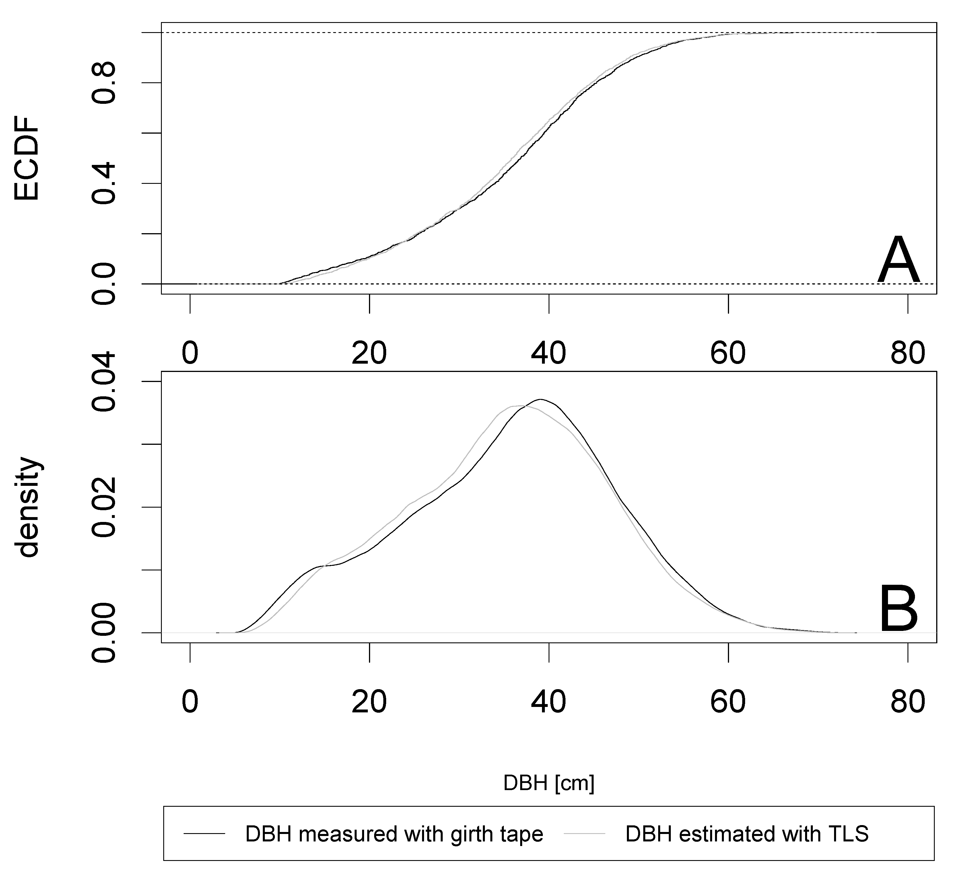
The empirical cumulative distribution functions (ECDF) and density functions of DBH values obtained from the TLS measurements, and those measured with girth tape in the field, are presented in Figure 3, corresponding descriptive statistics are presented in Table 3. According to a Kolmogorov-Smirnov-test, the two distributions do not differ significantly (), i.e., despite the relatively high RMSD, the new algorithms yielded a stand diameter distribution that is statistically equal to the one derived from the field map survey.
The basal area of the experimental stand was calculated as 45.7 m2 ha−1 and 46.9 m2 ha−1 based on TLS and FieldMap survey data respectively, this corresponds to a deviation of 1.2 m2 ha−1 or 2.6%.
3.3. Stand Mapping and Erosion
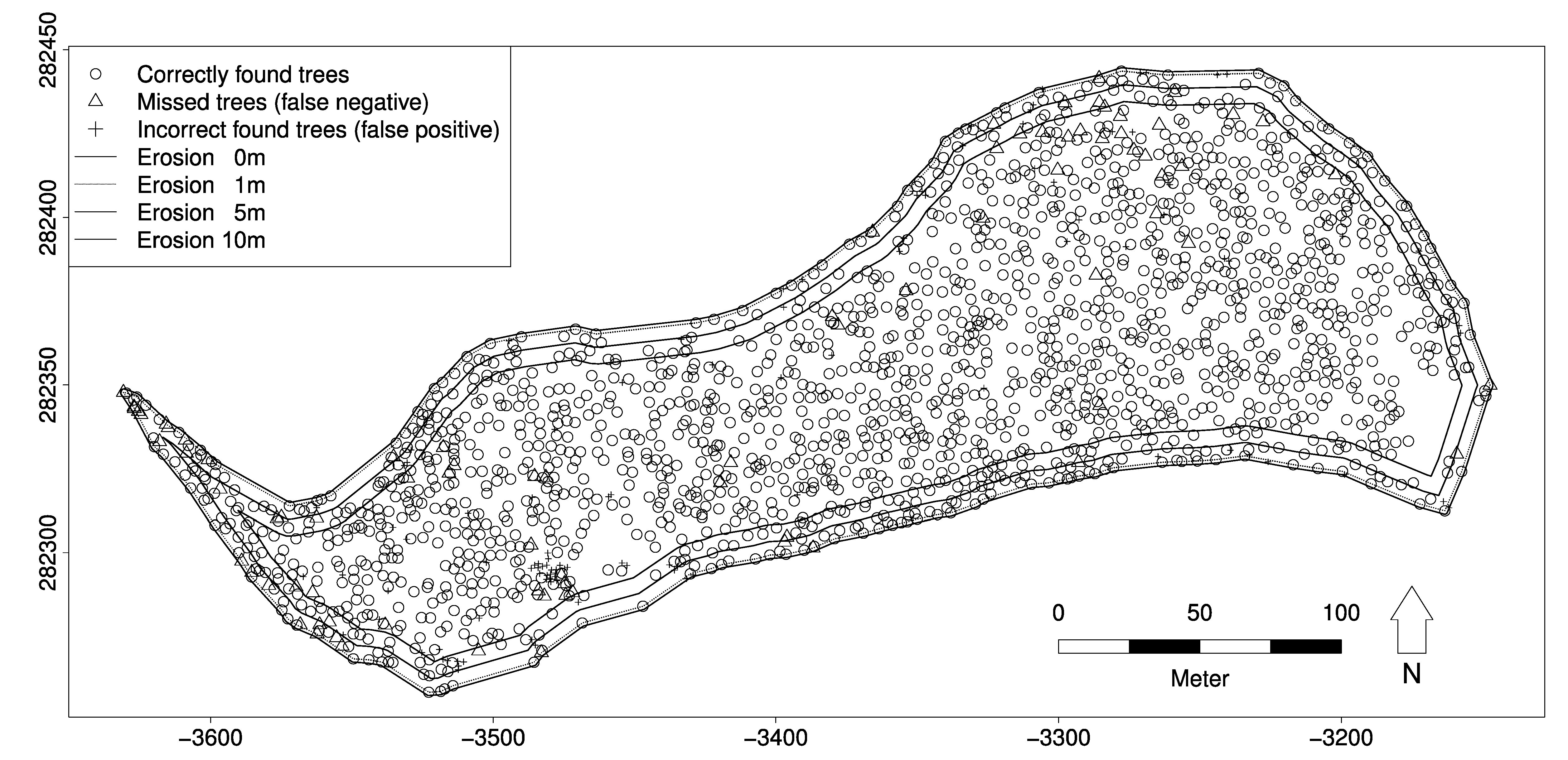
The map of tree positions (Figure 4) suggests that an edge effect exists and trees were more likely missed nearby the stand border. Moreover, the assumption that the detection rate might be higher for bigger trees seems intuitively reasonable.
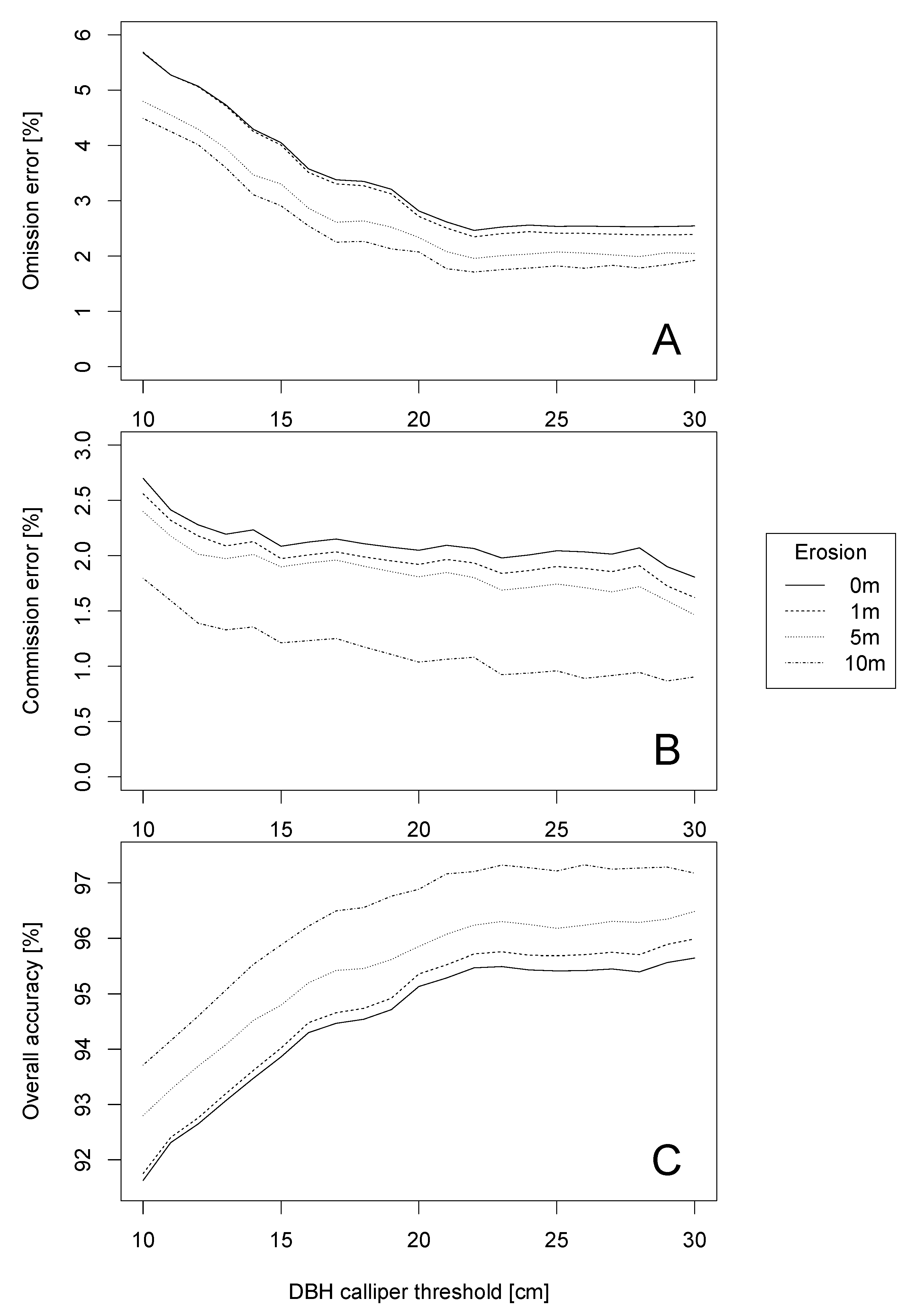
Figure 5 presents overall accuracy, commission error and omission error for an inner sub-window after removal of an outer buffer of varying size (different line types in Figure 5) and if only trees were considered having a DBH larger than a specific threshold (along the x-axis in Figure 5). Omission error and commission error decrease with increasing buffer size, and hence, overall accuracy increases with increasing buffer size. Omission error and commission error almost continuously decrease, and overall accuracy increases, with a DBH threshold increasing from 10 cm to 20 cm. Performance results do not change for any thresholds larger than 22 cm. When compared to the entire stand, application of a buffer of 10 m width increases overall accuracy by approx. 2 percentage points. Overall accuracy had its maximum of 97.2%, if a 10 m buffer was applied and if only trees were considered having a DBH larger than or equal to 21 cm.
4. Discussion
4.1. Subset from Point Clouds with Lower and Upper Limit
We made trials to find possible optima for a lower as well as an upper limit of a horizontal layer defining a subset from the entire point cloud on which the two-stage clustering algorithm for tree detection is applied. Because prior knowledge of existing tree locations was used in the optimization, general application of this procedure is not feasible when tree positions are predicted only from TLS data. However, results from our trial showed that the optimal layer for finding trees in point clouds is the space above the natural regeneration or ground vegetation and below the crowns. Thus, the lower limit should be set to a value high enough, so that most of the noise introduced by ground vegetation and natural regeneration is omitted. That is the case for a lower border of approx. 3 m in our study; further upwards shifts of the lower border had only small effects on the overall accuracy (Figure 1C). The upper border should be set to a value high enough, so that enough sublayers exist, and low enough, so that noise from tree crowns is minimized. The upper limit of the subset layer was set to 7.5 m, which corresponds to the 12.3%-quantile of the overstory crown base heights.
We would thus recommend that the field crews should sample some heights from understory vegetation and natural regeneration as well as from crown base heights of the overstory. As field crews have a break of approx. 11 min during every single scan (i.e., the time the devices needs to complete the scan), these additional measurements would consume no extra working time.
Trees with forked trunks might result in double detections if the bifurcation is below the upper limit of the horizontal layer. We therefore recommend that a bifurcation is treated as the crown base height during the sampling.
4.2. Transferability to Other Stands
Our novel methodology was so far only tested by means of a single but large and complex experimental stand. Transferability of the methods and results to other situations will be therefore examined in our future work. Our method (and TLS in general) is restricted in so far as stems as well as the reference markers must be visible from the scanner position. This might become problematic, e.g., in very dense pole stands or in tropical forests. However, feasibility of our approach was demonstrated in a complex scenario, with different tree species in a highly vertically structured stand and with presence of dense natural regeneration. It can be thus expected that the presented methodology should successfully work also in most forest landscapes in the temperate and boreal zones.
4.3. Estimation of DBH and Basal Area
The algorithm for automatic DBH estimation relies on prior knowledge of the maximum DBH in the stand, thus it is not feasible if only TLS data is available. However, field crews can use the 11 min scanning time to measure the DBH of the largest tree in sight. Based on these measurements and an additional safety margin of, e.g., 20%, the necessary information of the maximum DBH in the stand can be obtained without extra working time.
Despite the relatively high RMSD between the TLS-based automatic DBH estimates and the girth tape measurements, stand diameter distributions derived from the two approaches are statistically equal (Figure 3). The deviation between the basal area calculated from TLS and FieldMap survey data respectively, was only as 1.2 m2 ha−1 (i.e., 2.5%).
4.4. Verification of Automatically Detected Tree Positions
Due to the relatively long traverses required by the field work, tree coordinates from both the manual registration with FieldMap and the automatic TLS-based approach were affected by measurement error. Moreover, the TLS based approach derived the positions in a height of more than 4 m, so that for slanting trees there is a deviation to the position of the trunk base. Thus, a software algorithm had to be applied to map the point pattern derived from one measurement system to the pattern from the other system. As we had no prior experience with the applied automatic tree pattern algorithm, we have visually checked the mapping results in the 3D point cloud for all existing as well as proposed tree locations.
4.5. Edge Effects
As overall accuracy increased when results were evaluated on an inner sub-window, edge effects must have existed. One explanation is that the scanner could not be placed optimally nearby the stand borders, because restrictions were given by the steep terrain on embankments alongside the forest roads, which surround the experimental stand. Another possible explanation is the higher density of understory vegetation at the edges of the stand, due to the higher availability of light near the ground in this area. Moreover, TLS data collection had been aborted due to sudden rain falls. Therefore, the two final scans could not be completed. Consequently, there is a region with low TLS point density in the very northern part of the experimental stand, where the detection rate was very low.
4.6. Comparison with Other Studies
4.6.1. Tree Detection
In existing literature on automatic tree detection and mapping the overall accuracy and the detection rate are commonly used as performance measure. Our method achieved an overall accuracy between 91.6% for all trees having a DBH greater than or equal to 10 cm and 97.2% for trees with DBH greater than or equal to 21 cm standing on an inner sub-window after removal of an 10 m wide buffer zone; these coincide with detection rates of 94.3% and 98.2%, respectively.
The highest detection rate so far provided in existing literature is 100% reported by Maas et al. [44]; the corresponding overall accuracy is 92.8%. However, those results are based on one single 0.07 ha sample plot, containing only 14 trees (all of them 140 year old beeches), representing a very low tree density of only 200 trees ha−1. Other studies reported overall accuracies (the metric is called “completeness” in that reference) between 86.9% and 89.0% for dense but homogeneous bamboo stands [45] and detection rates of 90.4% in boreal coniferous forests [26] (the metric is called “recall” in that reference). Comparison of our multi-scan TLS based overall accuracies with measures obtained by single-scan TLS or airborne laser scanning (ALS) may be criticized as unfair, because the latter data are associated with lower measurement intensity. Nevertheless, the comparison is useful, as it demonstrates future capability of high resolution Lidar technology applied in forest monitoring practice in general.
Single-scan TLS is a time and cost efficient approach, however, it is limited to small sample plots, as the detection accuracy drastically decreases with increasing scanner to tree distance [46,47,48]. While distance sampling based approaches are able to correct for the non-detection, regarding estimates of the number of trees and the corresponding volume per ha [46,47], the observed tree pattern is thinned and remains incomplete. Thus, single-scan TLS cannot be applied for the mapping of entire forest stands.
Liang et al. [16] provide a comprehensive overview of detection rates reported in former studies. Hereby, single scan TLS generally yielded low detection rates between 22.0% and 72.3% [48,49,50,51,52,53,54,55]. However, one reference [44] reported extraordinary high detection rates between 86.7% and 100% (with corresponding overall accuracy of 73.3–96.5%) on three circular 0.07 ha plots in low-density forests.
ALS is even more time efficient than single scan TLS, as very large areas can be sampled in a very short time. However, the possible accuracy of ALS based tree detection is still insufficient for mapping experimental stands. As an example, Eysn et al. [56] reported omission errors between 42% and 65% and commission errors between 22% and 104%, while Dalponte et al. [57] reported overall accuracies (the metric is called accuracy index in that reference) between 30% and 44%.
4.6.2. DBH Measurement
Existing studies on DBH measurement from TLS have reported RMSD between measured and fitted DBH values ranging from 0.7 cm to 7.0 cm, and a corresponding bias between −1.6 cm and 1.6 cm [44,48,51,55]. This is on par with the results we could achieve with our new approach (RMSD = 4.95 cm, and bias = 0.38 cm). Our results did not outperform those from other existing applications, but our proposed approach has a relevant extra feature, as DBH can be estimated even under limited sighting conditions, when it cannot be measured directly.
5. Conclusions
We showed that TLS in multi-scan mode can be successfully applied for the automatic mapping of forest stands. The overall accuracy of up to 97.2% justifies operational use of TLS in forest monitoring.
Due to the fact that the highest overall accuracy was achieved for trees with DBH greater than or equal to 21 cm, we are confident that TLS can be applied in forest mensuration practice in the near future, because these larger trees represent the majority of growing stock volume.
Stem maps derived from TLS-based tree detection can be further used to collect additional information (e.g., tree species, health status, etc.) or to correct erroneous tree detections and DBH fits during traditional field surveys. Thus, TLS may not completely substitute traditional fieldwork, but will contribute to drastically enhance labor efficiency: TLS related field work took approx. one person-week, whereas the FieldMap survey took 24 person-weeks. Despite the need for additional working time for co-registration of the scans, TLS offers a great cost saving potential.
The complete workflow is based on established software products, there was no need for novel developments of programs or interfaces. Raw scanner data are manually co-registered in FARO Scene and the resulting point cloud is exported in standard xyz-format. Thus, data obtained with other instruments or co-registered within other software products, can also be used for further processing. All scripts for further processing are written in R, and the LASTools are directly invoked by system commands from within these R-scripts. We successfully tested our workflow under Windows (Microsoft Corporation, Redmond, Washington, USA) and GNU/Linux (Free Software Foundation, Boston, Massachusetts, USA) operating systems.
Long-term storage of the TLS point-cloud datasets should carefully be planned, as the required amount of storage capacity increases by six orders of magnitude compared to traditional measurements (the point-cloud of our experimental stand needs approx. 114 GB of storage capacity, whereas the FieldMap survey data just need 163 KB). To ensure long term data availability, we strongly recommend the use of standard and open data formats (like xyz-format), even though the necessary storage capacity is higher than for proprietary formats.
Another possible application of the new methods is change detection on already mapped stands. Using the automated tree detection and point assignment algorithms, it should be possible to detect the drop out of trees caused by harvesting or natural hazards, this would be a great tool for permanent monitoring of experimental stands.
Acknowledgments
The authors are grateful to Josef Gasch, head of the BOKU Forest Demonstration Centre, for his kind support and cooperativeness during the installation of the test site. The authors appreciate much the careful field work of Josef Paulic, Rudolph Feichter and Magdalena Höhne. The authors acknowledge the comments and suggestions provided by two anonymous reviewers.
Author Contributions
A.N. and T.R. designed the experiment; T.R. and M.S. performed the T.L.S. related field work and analyzed the data; A.N. and F.L. supported data analysis; all authors developed the tree detection algorithm; A.T., A.N., M.S. and T.R. programmed the tree detection algorithm; T.R. and A.N. developed and programmed the D.B.H. measuring algorithm; T.R. and M.S. drafted the manuscript.
Conflicts of Interest
The authors declare no conflict of interest.
Appendix

Table A1.
Step-by-step workflow and applied software functions and parameters.
| Step No. | Step/Sub-Step | Software | Package/Function | Parameters | ||
|---|---|---|---|---|---|---|
| 1 | Co-registration of scans | FARO Scene | ||||
| 2 | Export in .xyz format | |||||
| 3 | Import data | LAStools | txt2las | |||
| 4 | Coordinate transformation | las2las | - rotate_xy −8.25 0 0 - reoffset −3329.372 282345.7 0 | |||
| 5 | Thinning the point cloud | lasthin | - keep_every_nth 2 | |||
| 6 | Splitting point cloud into 1087 tiles | lastile | - tile_size 10 - buffer 2 | |||
| 7 | Filtering | lasnoise | - step 0.35 - isolation 850 | |||
| 8 | Differentiate between ground points and non-ground points. Normalize relative to the DEM | lasground | - step 1 - spike 0.4 - bulge 0.5 - offset 0.1 - replace z | |||
| 9 | Re-merge the tiles and remove the ground points | lastile | - drop_classification 2 | |||
| 10 | Splitting point cloud into 155 tiles | lastile | - tile_size 25 - buffer 5 | |||
| 11 | Export in txt format | las2txt | ||||
| 12 | Import data | R | data.table | fread() | ||
| 13a | Stage one clustering | Estimate cut off distance | densityClust | estimateDc() | NeighbourhoodRateLow = 0.005 NeighbourhoodRateHigh = 0.01 | |
| 13b | Calculate local density | densityClust() | Dc = [estimated dc from estimateDc()] | |||
| 13c | Find cluster centroids | findClusters() | rho = 2 delta = 0.5 | |||
| 14a | Stage two clustering | Calculate local density | densityClust | densityClust() | Dc = 0.04 | |
| 14b | Find cluster centroids | findClusters() | rho = 2 delta = 0.5 | |||
| 14c | Join clusters with a distance of less than 50 cm | spatstat | connected.ppp() | R = 0.5 | ||
| 15a | Assignment of tree locations | Construct -convex hull | alphahull | ahull() | Alpha = 30 | |
| 15b | Point assignment | spatstat | pppdist() | Cutoff = 1.5 | ||
| 16a | Diameter estimation | DBH | edci | circMclust() | Nx = 25 ny = 25 nr = 5 | |
| conicfit | LMcircleFit | |||||
| EllipseDirectFit | ||||||
| 16b | Upper Diameter | edci | circMclust() | Nx = 25 ny = 25 nr = 5 | ||
| conicfit | LMcircleFit | |||||
| EllipseDirectFit | ||||||
References
- Köhl, M.; Magnussen, S.S.; Marchetti, M. Sampling Methods, Remote Sensing and GIS Multiresource Forest Inventory; Springer-Verlag: Berlin/Heidelberg, Germany, 2006; ISBN 978-3-540-32572-7. [Google Scholar]
- MCPFE. Background information for improved Pan-European indicators for sustainable forest management. In Proceedings of the Ministerial Conference on the Protection of Forests in Europe (MCPFE) Liaison Unit, Vienna, Austria, 7–8 October 2002. [Google Scholar]
- MCPFE. State of Europe’s Forests 2003: The MCPFE report on sustainable forest management in Europe. In Proceedings of the Ministerial Conference on the Protection of Forests in Europe (MCPFE) Liaison Unit, Vienna, Austria, 28–30 April 2003. [Google Scholar]
- IUFRO. Guidelines for Designing Multipurpose Resource Inventories: A Project of IUFRO Research Group 4.02.02; Lund, H.G., Ed.; IUFRO World Series: Vienna, Austria, 1998; Volume 8. [Google Scholar]
- Kenning, R.S.; Ducey, M.J.; Brissette, J.C.; Gove, J.H. Field efficiency and bias of snag inventory methods. Can. J. For. Res. 2005, 35, 2900–2910. [Google Scholar] [CrossRef]
- Næsset, E. Predicting forest stand characteristics with airborne scanning laser using a practical two-stage procedure and field data. Remote Sens. Environ. 2002, 80, 88–99. [Google Scholar] [CrossRef]
- Maltamo, M.; Bollandsås, O.M.; Gobakken, T.; Næsset, E. Large-scale prediction of aboveground biomass in heterogeneous mountain forests by means of airborne laser scanning. Can. J. For. Res. 2016, 1144, 1138–1144. [Google Scholar] [CrossRef]
- De Vries, W.; Vel, E.; Reinds, G.J.; Deelstra, H.; Klap, J.M.; Leeters, E.E.J.M.; Hendriks, C.M.A.; Kerkvoorden, M.; Landmann, G.; Herkendell, J.; et al. Intensive monitoring of forest ecosystems in Europe 1. Objectives, set-up and evaluation strategy. For. Ecol. Manag. 2003, 174, 77–95. [Google Scholar] [CrossRef]
- Mellert, K.H.; Deffner, V.; Küchenhoff, H.; Kölling, C. Modeling sensitivity to climate change and estimating the uncertainty of its impact: A probabilistic concept for risk assessment in forestry. Ecol. Modell. 2015, 316, 211–216. [Google Scholar] [CrossRef]
- IFER. Field-Map—Tool Designed for Computer Aided Field Data Collection. Available online: http://www.fieldmap.cz/ (accessed on 28 February 2017).
- Field, H.L. Landscape Surveying; Cengage Learning: Delmar, CA, USA, 2012; ISBN 1111310602. [Google Scholar]
- Culvenor, D.S. TIDA: An algorithm for the delineation of tree crowns in high spatial resolution remotely sensed imagery. Comput. Geosci. 2002, 28, 33–44. [Google Scholar] [CrossRef]
- Pouliot, D.; King, D.; Bell, F.; Pitt, D. Automated tree crown detection and delineation in high-resolution digital camera imagery of coniferous forest regeneration. Remote Sens. Environ. 2002, 82, 322–334. [Google Scholar] [CrossRef]
- Ke, Y.; Quackenbush, L.J. A review of methods for automatic individual tree-crown detection and delineation from passive remote sensing. Int. J. Remote Sens. 2011, 32, 4725–4747. [Google Scholar] [CrossRef]
- Van Leeuwen, M.; Nieuwenhuis, M. Retrieval of forest structural parameters using LiDAR remote sensing. Eur. J. For. Res. 2010, 129, 749–770. [Google Scholar] [CrossRef]
- Liang, X.; Kankare, V.; Hyyppä, J.; Wang, Y.; Kukko, A.; Haggrén, H.; Yu, X.; Kaartinen, H.; Jaakkola, A.; Guan, F.; et al. Terrestrial laser scanning in forest inventories. ISPRS J. Photogramm. Remote Sens. 2016, 115, 63–77. [Google Scholar] [CrossRef]
- Næsset, E.; Gobakken, T.; Holmgren, J.; Hyyppä, H.; Hyyppä, J.; Maltamo, M.; Nilsson, M.; Olsson, H.; Persson, Å.; Söderman, U. Laser scanning of forest resources: the nordic experience. Scand. J. For. Res. 2004, 19, 482–499. [Google Scholar] [CrossRef]
- Kwak, D.-A.; Lee, W.-K.; Lee, J.-H.; Biging, G.S.; Gong, P. Detection of individual trees and estimation of tree height using LiDAR data. J. For. Res. 2007, 12, 425–434. [Google Scholar] [CrossRef]
- Ferraz, A.; Bretar, F.; Jacquemoud, S.; Gonçalves, G.; Pereira, L.; Tomé, M.; Soares, P. 3-D mapping of a multi-layered Mediterranean forest using ALS data. Remote Sens. Environ. 2012, 121, 210–223. [Google Scholar] [CrossRef]
- Kaartinen, H.; Hyyppä, J.; Yu, X.; Vastaranta, M.; Hyyppä, H.; Kukko, A.; Holopainen, M.; Heipke, C.; Hirschmugl, M.; Morsdorf, F.; et al. An international comparison of individual tree detection and extraction using airborne laser scanning. Remote Sens. 2012, 4, 950–974. [Google Scholar] [CrossRef] [Green Version]
- Vauhkonen, J.; Ene, L.; Gupta, S.; Heinzel, J.; Holmgren, J.; Pitkanen, J.; Solberg, S.; Wang, Y.; Weinacker, H.; Hauglin, K.M.; et al. Comparative testing of single-tree detection algorithms under different types of forest. Forestry 2012, 85, 27–40. [Google Scholar] [CrossRef]
- Maack, J.; Lingenfelder, M.; Weinacker, H.; Koch, B. Modelling the standing timber volume of Baden-Württemberg—A large-scale approach using a fusion of Landsat, airborne LiDAR and National Forest Inventory data. Int. J. Appl. Earth Obs. Geoinf. 2016, 49, 107–116. [Google Scholar] [CrossRef]
- Deo, R.K.; Froese, R.E.; Falkowski, M.J.; Hudak, A.T. Optimizing variable radius plot size and LiDAR resolution to model standing volume in conifer forests. Can. J. Remote Sens. 2016, 42, 428–442. [Google Scholar] [CrossRef]
- Scrinzi, G.; Clementel, F.; Floris, A. Angle count sampling reliability as ground truth for area-based LiDAR applications in forest inventories. Can. J. For. Res. 2015, 45, 506–514. [Google Scholar] [CrossRef]
- Srinivasan, S.; Popescu, S.C.; Eriksson, M.; Sheridan, R.D.; Ku, N.-W.; Waser, L.T.; Wynne, R.H.; Thenkabail, P.S. Terrestrial laser scanning as an effective tool to retrieve tree level height, crown width, and stem diameter. Remote Sens. 2015, 7, 1877–1896. [Google Scholar] [CrossRef]
- Yang, B.; Dai, W.; Dong, Z.; Liu, Y. Automatic forest mapping at individual tree levels from terrestrial laser scanning point clouds with a hierarchical minimum cut method. Remote Sens. 2016, 8, 372. [Google Scholar] [CrossRef]
- Hager, H. Die Klimastationen im lehrforst der universität für bodenkultur. Allg. Forstzeitung 1980, 91, 54–57. [Google Scholar]
- Glatzel, G.; Sieghardt, M. Die Böden des Lehrforstes. Allg. Forstztg. 1980, 91, 53–54. [Google Scholar]
- Haglöf Measurement Solutions in Forest and Field. Available online: http://www.haglofcg.com/index.php/en/products/instruments/height/341-vertex-iv (accessed on 17 March 2017).
- FARO Laser Scanner FARO Focus3D—Overview—3D Surveying. Available online: http://www.faro.com/en-us/products/3d-surveying/faro-focus3d/overview (accessed on 28 February 2017).
- FARO FARO Laser Scanner Software—SCENE—Overview. Available online: http://www.faro.com/en-us/products/faro-software/scene/overview (accessed on 28 February 2017).
- Isenburg, M. LAStools—Efficient LiDAR Processing Software (version 160429, Academic). Available online: https://rapidlasso.com/lastools/ (accessed on 28 February 2017).
- R Development Core Team. R: A Language and Environment for Statistical Computing, R Version 3.3.2; R Foundation for Statistical Computing: Vienna, Austria, 2016.
- Rodriguez, A.; Laio, A. Clustering by fast search and find of density peaks. Science 2014, 344, 1492–1496. [Google Scholar] [CrossRef] [PubMed]
- Pedersen, T.L.; Hughes, S. Densityclust: Clustering by Fast Search and Find of Density Peaks, R package version 0.2.1; 2016. Available online: https://cran.r-project.org/package=densityClust (accessed on 15 June 2017).
- Baddeley, A.; Rubak, E.; Turner, R. Spatial Point Patterns: Methodology and Applications with R; Chapman and Hall/CRC Press: London, UK, 2015. [Google Scholar]
- Edelsbrunner, H.; Kirkpatrick, D.; Seidel, R. On the shape of a set of points in the plane. IEEE Trans. Inf. Theory 1983, 29, 551–559. [Google Scholar] [CrossRef]
- Pateiro-Lopez, B.; Rodriguez-Casal, A. Alphahull: Generalization of the Convex Hull of a Sample of Points in the Plane, R package version 2.1; 2016. Available online: https://cran.r-project.org/package=alphahull (accessed on 15 June 2017).
- Müller, C.H.; Garlipp, T. Simple consistent cluster methods based on redescending M-estimators with an application to edge identification in images. J. Multivar. Anal. 2005, 92, 359–385. [Google Scholar] [CrossRef]
- Garlipp, T. Edci: Edge Detection and Clustering in Images. 2016. Available online: https://CRAN.R-project.org/package=edci (accessed on 17 June 2017).
- Chernov, N. Circular and Linear Regression: Fitting Circles and Lines by Least Squares; CRC Press: Taylor & Francis Group, Boca Raton, Florida, USA, 2011; ISBN 9781439835906. [Google Scholar]
- Gama, J.; Chernov, N. Conicfit: Algorithms for Fitting Circles, Ellipses and Conics Based on the Work by Prof. Nikolai Chernov, R package version 1.0.4; 2015. Available online: https://CRAN.R-project.org/package=conicfit (accessed on 17 June 2017).
- Fitzgibbon, A.W.; Pilu, M.; Fisher, R.B. Direct least squares fitting of ellipses. IEEE Trans. Pattern Anal. Mach. Intell. 1996, 21, 476–480. [Google Scholar] [CrossRef]
- Maas, H.-G.; Bienert, A.; Scheller, S.; Keane, E. Automatic forest inventory parameter determination from terrestrial laser scanner data. Int. J. Remote Sens. 2008, 29, 1593–1879. [Google Scholar] [CrossRef]
- Xia, S.; Wang, C.; Pan, F.; Xi, X.; Zeng, H.; Liu, H. Detecting stems in dense and homogeneous forest using single-scan TLS. Forests 2015, 6, 3923–3945. [Google Scholar] [CrossRef]
- Astrup, R.; Ducey, M.J.; Granhus, A.; Ritter, T.; von Lüpke, N. Approaches for estimating stand-level volume using terrestrial laser scanning in a single-scan mode. Can. J. For. Res. 2014, 44, 666–676. [Google Scholar] [CrossRef]
- Ducey, M.J.; Astrup, R. Adjusting for nondetection in forest inventories derived from terrestrial laser scanning. Can. J. Remote Sens. 2013, 39, 410–425. [Google Scholar]
- Olofsson, K.; Holmgren, J.; Olsson, H. Tree stem and height measurements using terrestrial laser scanning and the RANSAC algorithm. Remote Sens. 2014, 6, 4323–4344. [Google Scholar] [CrossRef]
- Thies, M.; Spiecker, H. Evaluation and future prospects of terrestrial laser scanning for standardized forest inventories. Int. Arch. Photogramm. Remote Sens. Spat. Inf. Sci. 2004, 36, 192–197. [Google Scholar]
- Strahler, A.H.; Jupp, D.L.; Woodcock, C.E.; Schaaf, C.B.; Yao, T.; Zhao, F.; Yang, X.; Lovell, J.; Culvenor, D.; Newnham, G.; et al. Retrieval of forest structural parameters using a ground-based lidar instrument (Echidna®). Can. J. Remote Sens. 2008, 34, 426–440. [Google Scholar] [CrossRef]
- Brolly, G.; Kiraly, G. Algorithms for stem mapping by means of terrestrial laser scanning. Acta Silv. Lign. Hung 2009, 5, 119–130. [Google Scholar]
- Murphy, G.E.; Acuna, M.A.; Dumbrell, I. Tree value and log product yield determination in radiata pine (Pinus radiata) plantations in Australia: comparisons of terrestrial laser scanning with a forest inventory system and manual measurements. Can. J. For. Res. 2010, 40, 2223–2233. [Google Scholar] [CrossRef]
- Lovell, J.L.; Jupp, D.L.B.; Newnham, G.J.; Culvenor, D.S. Measuring tree stem diameters using intensity profiles from ground-based scanning lidar from a fixed viewpoint. ISPRS J. Photogramm. Remote Sens. 2011, 66, 46–55. [Google Scholar] [CrossRef]
- Liang, X.; Litkey, P.; Hyyppa, J.; Kaartinen, H.; Vastaranta, M.; Holopainen, M. Automatic stem mapping using single-scan terrestrial laser scanning. IEEE Trans. Geosci. Remote Sens. 2012, 50, 661–670. [Google Scholar] [CrossRef]
- Liang, X.; Hyyppä, J. Automatic stem mapping by merging several terrestrial laser scans at the feature and decision levels. Sensors 2013, 13, 1614–1634. [Google Scholar] [CrossRef] [PubMed]
- Eysn, L.; Hollaus, M.; Lindberg, E.; Berger, F.; Monnet, J.-M.; Dalponte, M.; Kobal, M.; Pellegrini, M.; Lingua, E.; Mongus, D.; et al. A benchmark of lidar-based single tree detection methods using heterogeneous forest data from the alpine space. Forests 2015, 6, 1721–1747. [Google Scholar] [CrossRef] [Green Version]
- Dalponte, M.; Reyes, F.; Kandarre, K.; Gianelle, D. Delineation of individual tree crowns from ALS and hyperspectral data: A comparison among four methods. Eur. J. Remote Sens. 2015, 48, 365–382. [Google Scholar] [CrossRef]
Figure 1.
Accuracy of two-step clustering. (A): Omission error, (B): Commission error, (C): Overall accuracy.
Figure 1.
Accuracy of two-step clustering. (A): Omission error, (B): Commission error, (C): Overall accuracy.
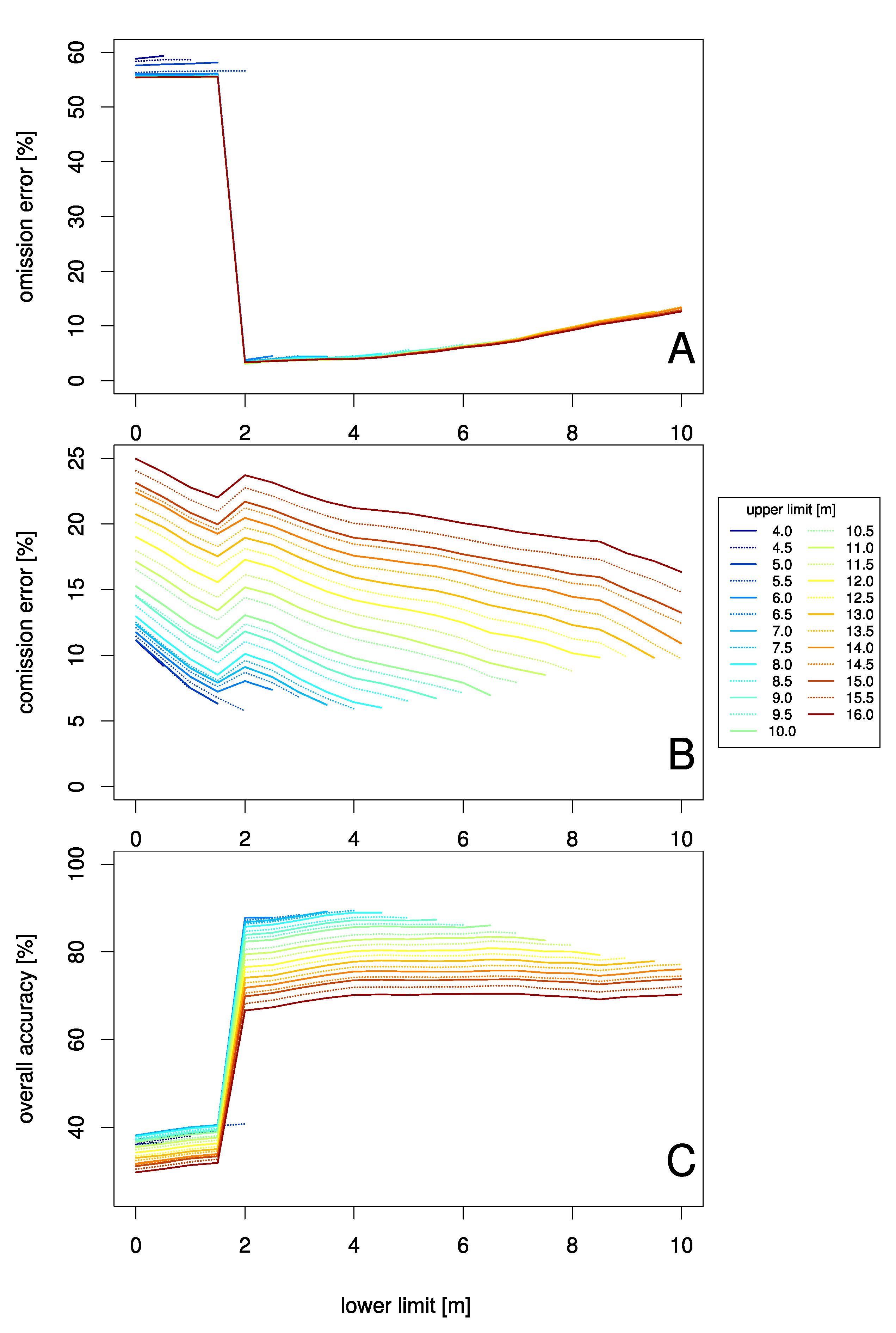
Figure 2.
Comparison of DBH values measured manually with girth tape, and those estimated automatically from the TLS data.
Figure 2.
Comparison of DBH values measured manually with girth tape, and those estimated automatically from the TLS data.
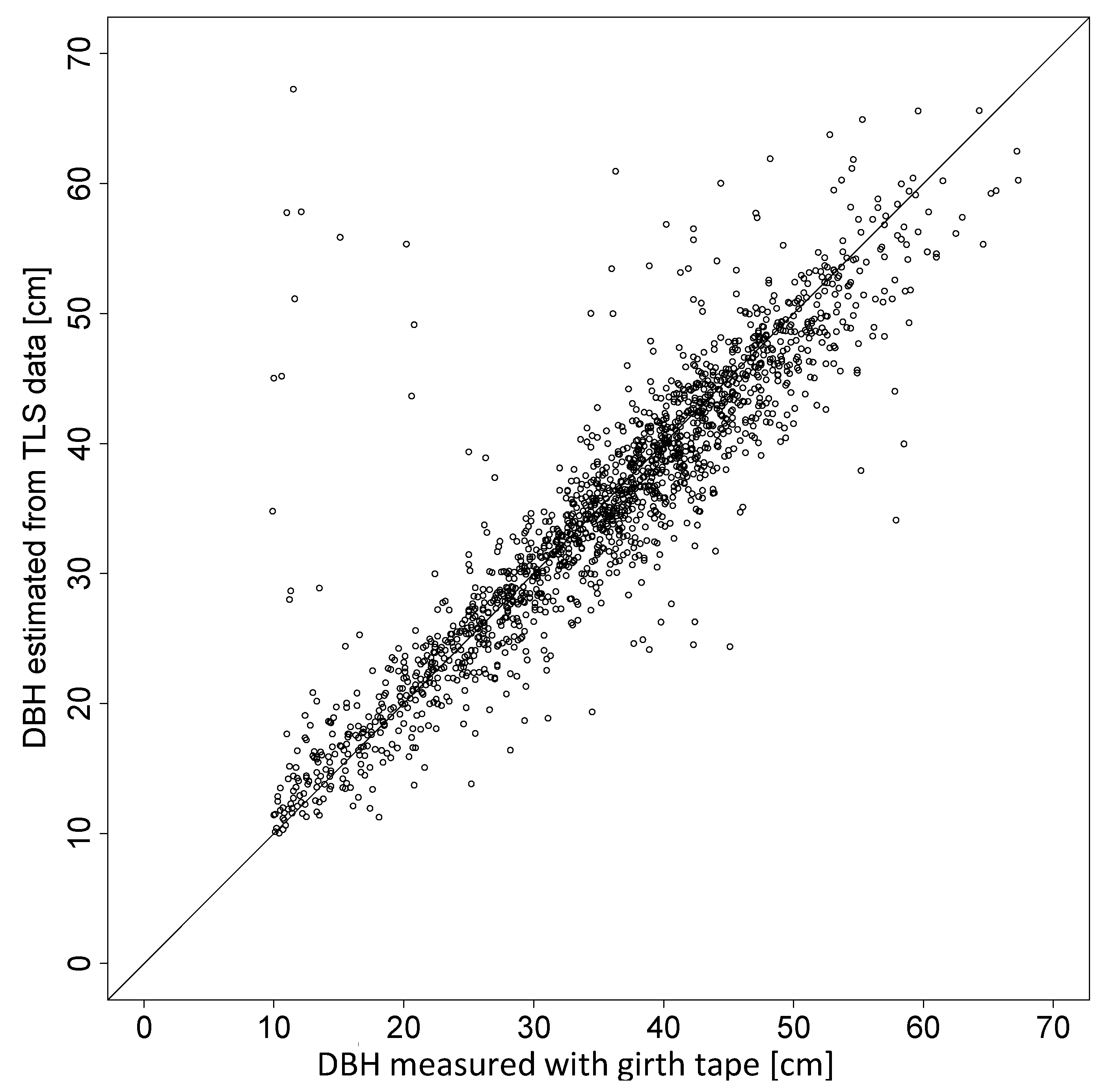
Figure 3.
Distribution of measured and fitted DBH-values. (A): ECDF = empirical cumulative distribution function (B): density = Epanechnikov kernel density estimation.
Figure 3.
Distribution of measured and fitted DBH-values. (A): ECDF = empirical cumulative distribution function (B): density = Epanechnikov kernel density estimation.

Figure 4.
Result of final tree mapping, WGS84 coordinates are in (m). Erosion indicates negative buffer-zones of 0 m, 1 m, 5 m, and 10 m width respectively that were used to account for possible edge effects.
Figure 4.
Result of final tree mapping, WGS84 coordinates are in (m). Erosion indicates negative buffer-zones of 0 m, 1 m, 5 m, and 10 m width respectively that were used to account for possible edge effects.

Figure 5.
Effect of erosion and calliper threshold on the accuracy (lower limit = 4 m, upper limit = 7.5 m) (A): Omission error, (B): Commission error, (C): Overall accuracy.
Figure 5.
Effect of erosion and calliper threshold on the accuracy (lower limit = 4 m, upper limit = 7.5 m) (A): Omission error, (B): Commission error, (C): Overall accuracy.

Table 1.
Parameter estimates for the coordinate transformation of the local coordinates from the FieldMap survey and from the terrestrial laser scanning (TLS) to WGS84.
Table 1.
Parameter estimates for the coordinate transformation of the local coordinates from the FieldMap survey and from the terrestrial laser scanning (TLS) to WGS84.
| (m) | (°) | ||
|---|---|---|---|
| FieldMap x-coordinate | −3612.23 | 1.003 | 3.24 |
| TLS x-coordinate | −3329.37 | 1.000 | 8.25 |
| FieldMap y-coordinate | 282,336.70 | 1.004 | 3.24 |
| TLS y-coordinate | 282,345.70 | 1.000 | 8.25 |
Table 2.
Number of trees sampled through the FieldMap survey and number of trees detected and missed by means of terrestrial laser scanning (TLS).
Table 2.
Number of trees sampled through the FieldMap survey and number of trees detected and missed by means of terrestrial laser scanning (TLS).
| Spruce | Fir | Larch | Pine | Beech | Other Broad Leaf | NA | Total | |
|---|---|---|---|---|---|---|---|---|
| FieldMap sampled | 684 | 259 | 65 | 91 | 678 | 12 | 1789 | |
| FieldMap corrected | 684 | 259 | 65 | 91 | 678 | 12 | 27 | 1816 |
| correct detections | 664 | 239 | 62 | 87 | 624 | 10 | 27 | 1713 |
| false positive detections | 49 | 49 | ||||||
| missed tree positions | 20 | 20 | 3 | 4 | 54 | 2 | 103 |
Table 3.
Descriptive statistics of TLS based DBH estimates and girth tape measurements.
| Min. (cm) | 1st Quartile (cm) | Median (cm) | 3rd Quartile (cm) | Max. (cm) | Mean (cm) | SD (cm) | |
|---|---|---|---|---|---|---|---|
| Girth tape measurements | 10.0 | 28.0 | 36.3 | 43.5 | 67.3 | 35.0 | 11.4 |
| TLS based estimates | 10.0 | 27.2 | 35.6 | 43.0 | 67.2 | 34.9 | 11.3 |
© 2017 by the authors. Licensee MDPI, Basel, Switzerland. This article is an open access article distributed under the terms and conditions of the Creative Commons Attribution (CC BY) license (http://creativecommons.org/licenses/by/4.0/).
Share and Cite
MDPI and ACS Style
Ritter, T.; Schwarz, M.; Tockner, A.; Leisch, F.; Nothdurft, A. Automatic Mapping of Forest Stands Based on Three-Dimensional Point Clouds Derived from Terrestrial Laser-Scanning. Forests 2017, 8, 265. https://doi.org/10.3390/f8080265
AMA Style
Ritter T, Schwarz M, Tockner A, Leisch F, Nothdurft A. Automatic Mapping of Forest Stands Based on Three-Dimensional Point Clouds Derived from Terrestrial Laser-Scanning. Forests. 2017; 8(8):265. https://doi.org/10.3390/f8080265
Chicago/Turabian StyleRitter, Tim, Marcel Schwarz, Andreas Tockner, Friedrich Leisch, and Arne Nothdurft. 2017. "Automatic Mapping of Forest Stands Based on Three-Dimensional Point Clouds Derived from Terrestrial Laser-Scanning" Forests 8, no. 8: 265. https://doi.org/10.3390/f8080265
Note that from the first issue of 2016, this journal uses article numbers instead of page numbers. See further details here.