Near-Real-Time Monitoring of Insect Defoliation Using Landsat Time Series

1
Department of Environmental Conservation, University of Massachusetts Amherst, 160 Holdsworth Way, Amherst, MA 01003, USA
2
Northeast Climate Science Center, University of Massachusetts Amherst, 233 Morrill Science Center, 611 North Pleasant Street, Amherst, MA 01003, USA
3
Department of Earth and Environment, Boston University, 675 Commonwealth Ave., Boston, MA 02215, USA
*
Author to whom correspondence should be addressed.
Forests 2017, 8(8), 275; https://doi.org/10.3390/f8080275
Submission received: 2 June 2017
/
Revised: 19 July 2017
/
Accepted: 22 July 2017
/
Published: 31 July 2017
(This article belongs to the Special Issue Remote Sensing of Forest Disturbance)
Abstract
:Introduced insects and pathogens impact millions of acres of forested land in the United States each year, and large-scale monitoring efforts are essential for tracking the spread of outbreaks and quantifying the extent of damage. However, monitoring the impacts of defoliating insects presents a significant challenge due to the ephemeral nature of defoliation events. Using the 2016 gypsy moth (Lymantria dispar) outbreak in Southern New England as a case study, we present a new approach for near-real-time defoliation monitoring using synthetic images produced from Landsat time series. By comparing predicted and observed images, we assessed changes in vegetation condition multiple times over the course of an outbreak. Initial measures can be made as imagery becomes available, and season-integrated products provide a wall-to-wall assessment of potential defoliation at 30 m resolution. Qualitative and quantitative comparisons suggest our Landsat Time Series (LTS) products improve identification of defoliation events relative to existing products and provide a repeatable metric of change in condition. Our synthetic-image approach is an important step toward using the full temporal potential of the Landsat archive for operational monitoring of forest health over large extents, and provides an important new tool for understanding spatial and temporal dynamics of insect defoliators.
1. Introduction
A growing number of introduced insects and pathogens threaten the health of forested ecosystems across North America, often with significant ecological and economic consequences [1,2,3,4]. Detecting and managing emerging outbreaks and predicting where outbreaks will occur in the future requires up-to-date spatially explicit information on the magnitude and extent of pest and disease impacts [5]. However, detecting changes in forest condition associated with insect pests over large extents remains an ongoing challenge [6].
Monitoring insect defoliation is particularly difficult due to the ephemeral nature of defoliation events. In the Northeastern US and parts of Canada, the gypsy moth (Lymantria dispar) has become a major forest pest following an accidental introduction near Boston in the late 1860s [3,7,8]. Gypsy moths are distinct among defoliators in that they feed on a wide variety of host trees and produce more extensive and severe defoliation than other native and non-native species [7]. Gypsy moths’ preferred hosts are hardwood trees, particularly oak (Quercus spp.) and aspen (Populus spp.), making the Northeast US particularly susceptible to outbreaks [9]. Gypsy moth caterpillars hatch from egg masses in early May, but defoliation is not usually noticeable until early or mid-June, and peak defoliation typically occurs by late June or early July [7,8]. While trees typically recover from individual events, repeated defoliation combined with other stressors may result in tree mortality, leading to long-term shifts in forest species composition [10,11,12]. Hundreds of thousands of hectares of forest are defoliated by gypsy moth each year and models suggest the species’ North American range will continue to expand [8,13,14]. Therefore, cost-effective, repeatable monitoring approaches are highly desirable for both early detection of new outbreaks as well as post-disturbance defoliation assessments.
Satellite remote sensing has long been recognized as a potential solution for mapping and monitoring changes in forest health, including identifying gypsy moth defoliation [15,16,17,18,19]. Most remote sensing studies approach defoliation as a change process, using two or more dates of imagery to differentiate between defoliated and non-defoliated conditions [3,20]. Products from the Landsat family of satellites are prevalent in studies of forest insect disturbance due to their moderate spatial resolution and long history of image acquisition [6]. The modern series of Landsat instruments collect “spectral bands” of visible, near-infrared, and short-wave infrared reflectance data at a 30 m × 30 m pixel resolution with images acquired at least every 16 days (and temporal coverage may be higher where images overlap and when multiple sensors are active). However, because of the ephemeral nature of defoliation events, cloud cover has remained a major concern effecting the use of Landsat imagery for operational forest health monitoring [15,17,20,21].
Clouds and cloud shadows can significantly reduce the useable data in a given image, and data loss due to even small clouds is compounded when comparing images from multiple dates to assess change. To minimize the impacts of clouds, past Landsat-based approaches for detecting gypsy moth defoliation have typically selected only the best available cloud-free imagery for analysis. As a result, estimates of defoliation based on annual imagery could miss peak defoliation, and change detection may be influenced by year-to-year variability in vegetation phenology [21]. Studies of broadleaf defoliators like the gypsy moth would benefit from denser time series that include intra-annual variation in spectral properties of the forest canopy [6].
In this study, we introduce a new approach for operational mapping and monitoring insect defoliation events using “synthetic” images derived from time series of all high-quality Landsat observations. Unlike best-available-pixel image composites, which are comprised of actual or transformed surface reflectance data from images acquired on different dates, cloud-free synthetic images are predicted data based on models fit to the historic record of observations for each pixel [22]. Synthetic images can be generated for any date and thus enable direct comparison between observed and predicted vegetation conditions any time a partially clear image is acquired.
We developed and tested our synthetic image monitoring approach in rapid response to the 2016 gypsy moth outbreak in Southern New England. Biocontrol agents have significantly reduced the frequency of outbreaks in New England following the last peak in the early 1980s, but a series of unusually dry springs (2014–2016) decreased the effectiveness of these agents, leading to a major outbreak beginning in early summer 2016. Using Landsat time series, we sought to (1) monitor defoliation patterns in near-real time; (2) assess both the magnitude and extent of impacts; and (3) produce seamless, cloud-free damage maps over multiple Landsat scenes. We compare our results with aerial sketch data and another Landsat-based forest health product to determine relative improvements in detecting and mapping defoliation. This research presents a novel approach for assessing the extent and magnitude of defoliation events, and addresses a recognized need for near-real-time monitoring and large-scale mapping of insect disturbances using remote sensing data [6].
2. Materials and Methods
We used both the Landsat historic record and newly acquired imagery to monitor the magnitude and extent of damage during the 2016 gypsy moth outbreak in Southern New England. Our approach for defoliation monitoring proceeded in three stages: (1) historic model fitting; (2) near-real-time monitoring of canopy condition; and (3) season-integrated defoliation assessment (workflow shown in Figure 1). Image processing and analysis were conducted with open source Python and GDAL software packages [23] and all datasets originating from this study have been deposited in a publicly accessible database [24].
2.1. Historic Model Fitting
Historic model fitting was performed using an archive of all available Landsat 4–5 TM, Landsat 7 ETM+, and Landsat 8 OLI surface reflectance products for two Landsat scenes: World Reference System 2 (WRS-2) Path 12/Row 31 and Path 13/Row 31. All images used in this study were Level 1 Terrain Corrected (L1T) Climate Data Record (CDR) products downloaded via the USGS Earth System Processing Architecture (ESPA) system [25].
Rather than select a single image or observation to serve as a non-defoliated baseline, we use time series of all high-quality cloud-free Landsat observations to model the average reflectance patterns for each individual pixel during a stable base period. Because gypsy moth populations in New England have not reached outbreak levels since the early 1980s, the Landsat TM/ETM+/OLI record (1984 to present) should not include any major gypsy moth defoliation events. Nonetheless, we defined the base period for this study to include only observations from January 2005 through December 2015. We assume this 11-year period provides a sufficient number of observations to characterize long-term seasonal dynamics, while minimizing processing time and reducing potential for other types of change in forest condition or land use to confound the defoliation signal.
We used a Python implementation of the Continuous Change Detection and Classification (CCDC) algorithm [26] described in [22,27,28] to fit harmonic models for each pixel in our Southern New England study area. We chose to model time series of Tasseled Cap Greenness (TCG), a physically-based transform that combines individual Landsat spectral bands into a single metric representative of vegetated greenness. While other studies have identified SWIR-based indices, such as the Normalized Difference Moisture Index (NDMI) or Tasseled Cap Wetness (TCW), as demonstrating superior performance in detecting defoliation [21,29], we have found that the seasonal signatures of vegetation-sensitive indices such as TCG are better represented by harmonic models (see [30] for comparison of seasonal patterns).
We calculated TCG for all Landsat images using the Landsat TM surface reflectance transform coefficients [31]. We selected these coefficients because they were derived specifically for surface reflectance data, and they have been widely used in other studies combining data from multiple Landsat sensors (e.g., [32,33]). We acknowledge that spectral differences between Landsat sensors may influence TCG calculations; however, based on comparisons presented by [33,34], we assume that any cross-sensors differences are small relative to the observed defoliation signal and will not have a significant impact on assessment results. Therefore, we directly integrated Landsat TM, ETM+, and OLI data in our time series analysis.
CCDC models were fit to time series of Tasseled Cap Greenness observations from the 2005–2015 base period using a Fourier-style regression model. We chose to use harmonic regression over other non-parametric models and data filters because harmonic models (1) characterize general seasonal patterns across years, (2) produce a fitted equation for each pixel that can be used for predicting images at any given day of year, and (3) are becoming more widely used for operational monitoring of land cover, condition, and change [27,28,34,35]. The models used in this study included 12-month and 4-month harmonics based on the following functional form:
where is the ordinal date of each observation; is the modeled intercept; is the modeled slope; N is a set of integers specifying the frequency, j, of the Fourier series harmonics (N = {1, 3}, corresponding to 12-month and 4-month harmonics); are the sine coefficients and are the cosine coefficients estimated at each frequency; T is the number of days in a year (T = 365.25); and is the residual error term for each observation.
CCDC modeling was performed in two stages. First, model fitting is used to identify stable land cover segments and potential points of change using a Least Absolute Shrinkage and Selection Operator (LASSO) regression analysis method. Though LASSO and other robust regression methods that penalize the absolute size of the regression coefficients are preferred for change detection analysis [28], these methods result in coefficients that are biased toward smaller values. Therefore, we added a second stage to the general CCDC workflow where we re-fit stable model periods identified by the initial CCDC run using Ordinary Least Squares (OLS) regression. This re-fit step allowed us to generate unbiased estimates of regression coefficients and residuals that are more suitable for our condition analysis.
The model results included the fitted harmonic coefficients, as well as an estimate of the model Root Mean Squared Error (RMSE) for each pixel in the study area. While exceptionally wet or dry years may result in short-term changes in reflectance not related to defoliation, the harmonic modeling approach provides a relatively stable estimate of long-term reflectance patterns, and the RMSE estimate characterizes the baseline level of inter-annual variability and general signal noise in each time series, providing a point of comparison for detecting above-average levels of canopy change falling at the tails of the expected error distribution. Additionally, the harmonic models fit using the CCDC approach include a slope term that explicitly accounts for long-term trends such as forest growth or stress.
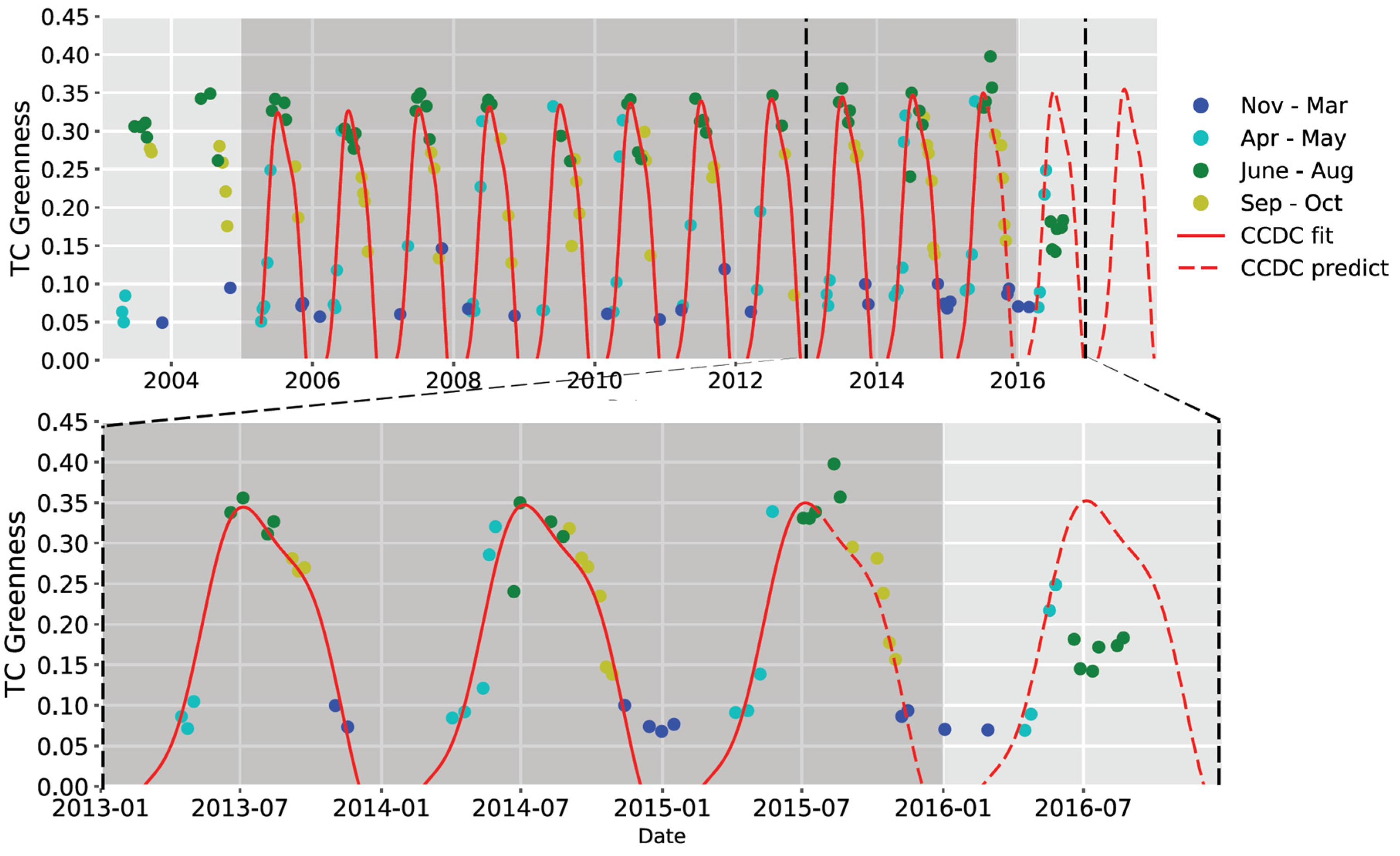
Figure 2 shows the CCDC model fitting (2005–2015) and prediction (2016–2017) for an example pixel. The model fitting results are visualized spatially as synthetic images, which predict TCG values for particular dates. Because they are based on time series of seasonal observations, synthetic images are not influenced by clouds and inherently account for seasonal variability in reflectance, and can therefore be used to estimate potential defoliation any day a Landsat image is acquired.
2.2. Near-Real-Time Monitoring
To assess defoliation in near-real-time during the outbreak period (early June through mid-September 2016), we acquired new Landsat images as they became available in the ESPA On-Demand Interface [25]. Though our methodology does not require we minimize cloud cover, we selected images of relatively good quality and well-suited for assessing condition, e.g., large contiguous areas of forested land visible, low overall cloud cover, and/or cumulus clouds easily removed using automated cloud masking. For acquisitions that were determined to be sufficiently clear, we downloaded the image and calculated TCG. We compared each TCG “observed” image from the monitoring period to a “predicted” synthetic TCG image created for the same day of year.
We estimated forest “condition” by differencing the observed and predicted TCG values for each pair of observed and predicted images. To convert these raw differences into a score that can be compared across images, we standardized the raw difference in TCG by dividing by the root mean squared error (RMSE) of the harmonic model for each pixel (Figure 1). The RMSE standardization creates a continuous condition score whose units indicate deviations in observed TCG relative to unexplained variability in the time series model. Though condition scores were initially calculated for all pixels, we applied a forest/non-forest mask based on the 2011 National Land Cover Dataset (NLCD) to limit our interpretation to only forested areas.
2.3. Season-Integrated Defoliation Assessment
In the final stage of our analysis, all near-real-time condition scores were combined to produce an integrated assessment of potential defoliation for the outbreak period. Because our two study scenes are in different UTM Zones, we re-projected all near-real-time assessments to Albers Equal Area Conic projection (EPSG: 5070) using nearest neighbor resampling. As a result of this pixel-level integration, areas where Landsat Paths overlapped had up to twice as many scores as areas within a single image. Though the minimum or a percentile could be used to identify the lowest condition score (i.e., largest difference between observed and predicted vegetation greenness) for each pixel, missed cloud shadows were found to produce large single-date changes in condition scores in areas that otherwise appeared to be undisturbed. Therefore, we averaged all available near-real-time condition scores for each pixel to reduce noise and identify pixels with persistently negative condition scores likely to be associated with defoliator activity. The final season-integrated assessment provides a seamless, cloud-free estimate of potential defoliation for the full study area.
2.4. Comparison to Existing Defoliation Products
While ground-based measurements are considered the gold standard for map accuracy assessment, the ephemeral, large-scale nature of gypsy moth defoliation events make it difficult to establish a proper validation sample. Furthermore, direct estimates of percent defoliation would require a multi-year ground campaign to estimate a baseline of “normal” canopy characteristics with which defoliated conditions could be compared. Given that this work was conducted in rapid response to an unfolding event, we focus instead on the quality and utility of our results relative to existing defoliation products via a series of map-to-map comparisons.
We compared our season-integrated defoliation assessment, hereafter referred to as the Landsat Time Series (LTS) product, with two other defoliation products: (1) U.S. Forest Service (USFS) aerial sketch maps of gypsy moth defoliation, and (2) a remote sensing-based USFS Forest Health Technology Enterprise Team (FHTET) defoliation product.
The aerial sketch map data represent the current standard for spatial assessment of gypsy moth damage. We obtained 2016 gypsy moth defoliation sketch polygons from the USFS Durham, NH Field Office. Survey flights were conducted on multiple dates between 21 June 2016 and 25 August 2016. Specific survey approaches varied by state, and included both hand-digitized polygons representing the general boundaries of defoliated areas, as well as assessments of regularly spaced grid cells. Five levels of defoliation were assigned by aerial interpreters: very severe, severe, moderate, light, and very light.
The FHTET product, which is also based on Landsat imagery, represents a new forest health monitoring approach currently being piloted for operational use [36]. This product uses a multi-date statistical (Z-score) change detection approach where imagery from the current year is compared with a baseline image for the same time of year from three previous years. We obtained three FHTET datasets, including raw results, as well as two additional maps (Sieve 1 and Sieve 2) that had been post-processed using sieving, a technique for spatially filtering categorical raster data to remove isolated pixels. All FHTET datasets used in our comparison specified two categories: “disturbed” and “undisturbed”, though it should be noted that the Z-scores used to determine these categories would be a continuous metric.
To characterize differences between the LTS product and the aerial sketch and FHTET defoliation products, we generated histograms showing the distributions of mean LTS condition scores within and outside areas labeled as defoliated by the other datasets. In the case of the sketch polygons, we considered four levels of defoliation: (1) very severe; (2) severe; (3) moderate; and (4) very light/light. In the case of the FHTET data, we considered the raw FHTET data and both sieved products. Non-forested pixels were excluded from this analysis. Additionally, we compared mapped results across all three products to provide spatial context. As a final point of comparison, we used the three defoliation products considered in this study to estimate the potential area of gypsy moth defoliation that occurred in the state of Rhode Island.
3. Results
3.1. Mapping and Monitoring
Using near-real-time assessments, we were able to monitor the spatial distribution and temporal persistence of changes in forest condition over the course of the 2016 gypsy moth outbreak. We generated 16 near-real-time assessments for our Southern New England study area, including seven dates from WRS-2 Path 12/Row 31 and nine dates from Path 13/Row 31 (Table 1). The first signs of gypsy moth damage were evident in assessments from 18 June (Path 13/Row 31) and 19 June (Path 12/Row 31). As expected, defoliation resulted in large negative condition scores, indicating a decrease in vegetation greenness relative to the modeled prediction.
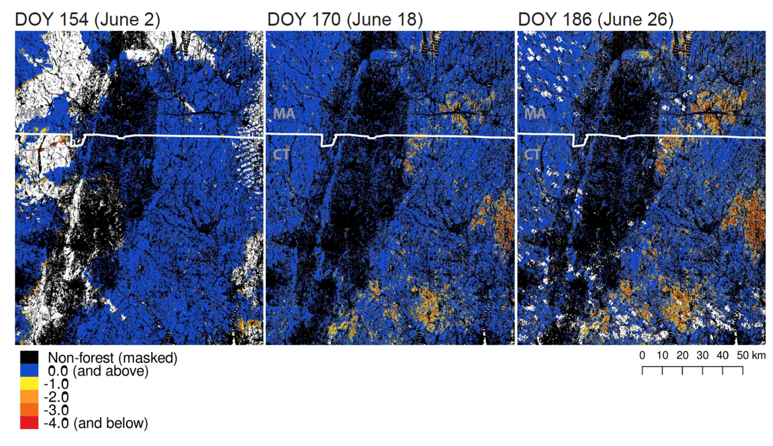
Figure 3 shows a series of three near-real-time assessments for the Connecticut River Valley. The 2 June assessment, which was not included in our final defoliation analysis, includes large areas of missing data (white areas) resulting from cloud/cloud shadow masking, but the remaining condition scores are near zero (blue), with the exception of some more negative scores along the edges of masked areas. By 18 June, several areas with large negative condition scores become apparent. Unlike the masking artifacts in the 2 June image, negative scores persist through 26 June, highlighting defoliation events in near-real time. Near-real-time results from August and September also revealed condition scores becoming less negative toward the end of the monitoring period, suggesting that we are able to characterize the timing and magnitude of the initial outbreak, as well as recovery dynamics.
The 2016 LTS season-integrated assessment averages potential changes in condition over the monitoring period, providing a wall-to-wall map for the full study area (Figure 4). Negative condition scores tend to form large coherent patches expected with gypsy moth activity. Furthermore, condition scores exhibit a gradient of values, suggesting field data could eventually be used to establish a relationship between the magnitude of LTS condition scores and severity of defoliation in terms of percent canopy loss or trees affected.
3.2. Comparison with Other Defoliation Products
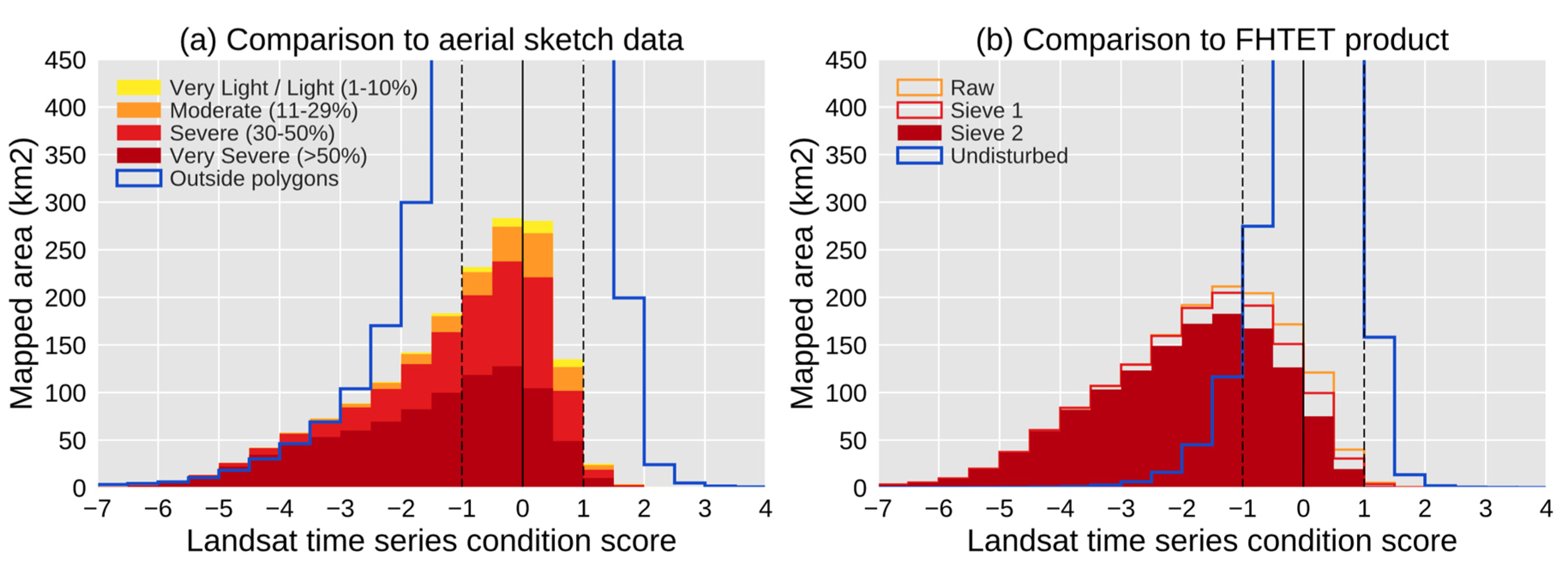
The distributions of LTS condition scores inside and outside of aerial sketch polygons both peak between −1.0 and 1.0 (Figure 5a), suggesting that defoliation polygons include a large number of pixels where condition scores indicate little or no difference in canopy greenness. Polygons labeled “very severe” (>50% defoliated) tended to include the largest area with negative condition scores, followed by polygons labeled “severe” (30–50% defoliated). However, a large portion of the study area (about 1320 km2) with LTS condition scores less than −1.0 was not identified as defoliated in the aerial sketch map. In fact, the area covered by pixels with condition scores less than −3.0, which indicate large, persistent deviations from predicted greenness beyond the expected model error, is approximately the same outside the aerial sketch polygons (197 km2) as inside (223 km2). At the same time, aerial sketch polygons include 749 km2 of forested area with LTS condition scores of −1.0 and greater, indicating that aerial sketch data include a large portion of forest where little to no change in condition was observed in the LTS assessment.
Unlike the aerial sketch results, the distributions of LTS condition scores for pixels mapped as “disturbed” and “undisturbed” in the FHTET data have distinct peaks, with disturbed pixels exhibiting larger negative LTS condition scores (Figure 5b). Comparing histograms for the three FHTET products, we find that sieving tended to reduce total area with condition scores between −1.0 and 1.0, suggesting that post-processing effectively removes pixels in locations where LTS condition scores do not indicate defoliation. However, sieving also reduced the overall area with condition scores less than −1.0, suggesting pixels where LTS condition scores do indicate a notable change in canopy greenness are also removed.
Comparing the LTS, aerial sketch and FHTET Sieve 2 products spatially (Figure 6) further contextualizes the results of the histogram comparisons. Hand-digitized aerial sketch polygons include large areas where LTS condition scores suggest no change in reflectance has occurred, while at the same time some areas with negative condition scores are missed entirely. This reflects the challenges of using a subjective sketch map approach for detailed event mapping.
The two Landsat-based products provide a more objective estimate of defoliation, and not surprisingly had much higher agreement, with the FHTET product including a greater area with LTS condition scores less than −3.0 while excluding more area with LTS condition scores greater than −1.0. The FHTET product provides more precise mapping of defoliated areas than the aerial polygons, and tends to include areas with the most negative LTS condition scores. However, the FHTET product appears to miss large areas of light to moderate defoliation with LTS condition scores between −2.0 and −1.0. There are also places where the FHTET product suggests disturbance, while the LTS product does not. These results suggest that while both Landsat-based approaches generally identify similar areas of high-magnitude change in reflectance, there remain notable differences in final mapped products.
3.3. State-Level Defoliation Assessment: Rhode Island
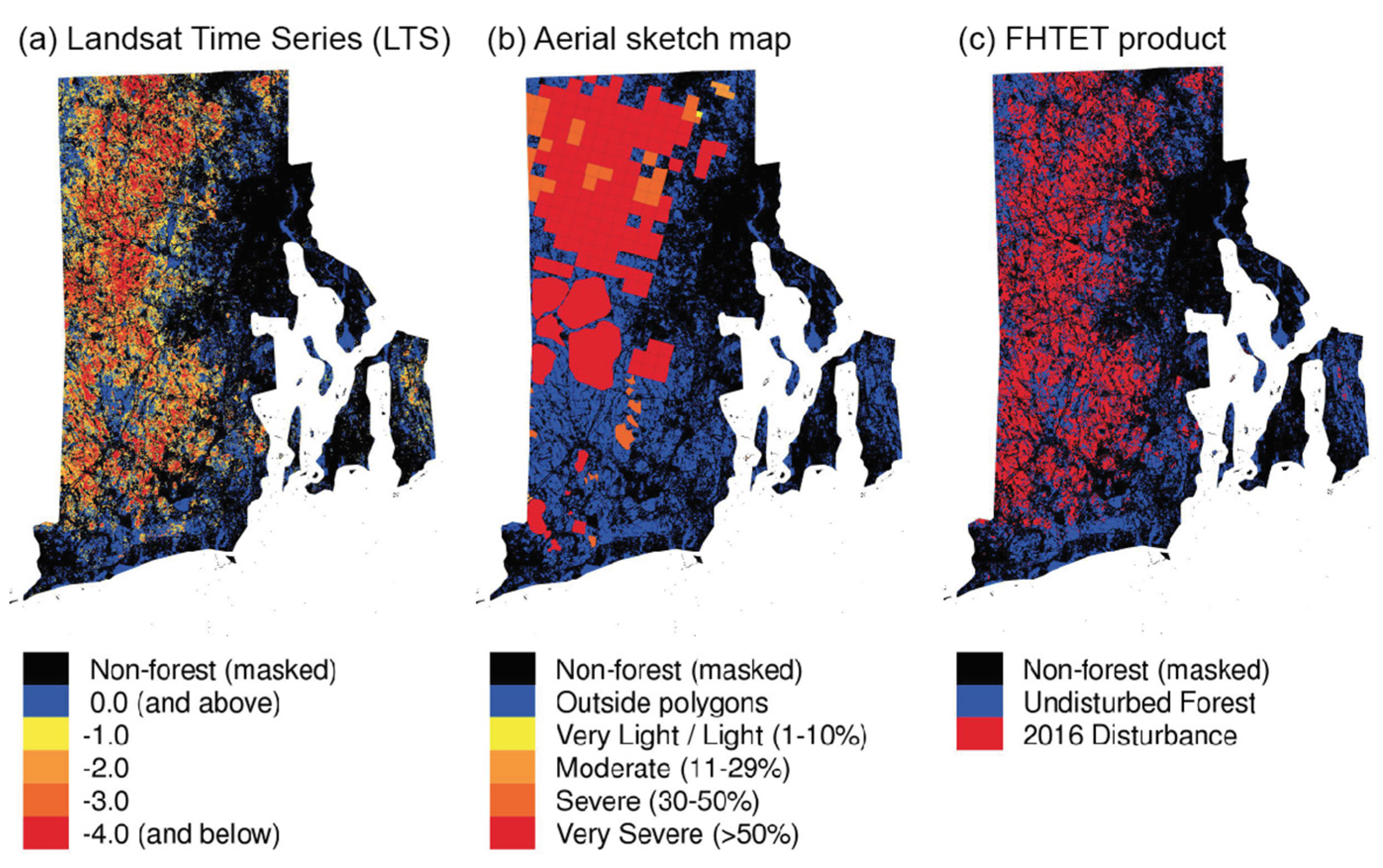
Rhode Island experienced some of the heaviest and most widespread defoliation during the 2016 outbreak (Figure 4). Total affected area varied considerably depending on the product and level of damage considered (Table 2). The FHTET product had the highest overall estimate of defoliated area (641 km2), followed by the LTS product where condition scores are less than or equal to −1 (618 km2), then the areas from aerial sketch maps at various thresholds (525 km2). The area estimates from our LTS products showed considerably more variability than the aerial sketch data at different levels of estimated defoliation, with total area affected ranging from 220 km2 (17.6% of total forested area) where condition scores were less than −3.0, to 618 km2 (49.3%) where condition scores were less than −1.0. Though the maximum defoliated area estimates for all three products are relatively comparable, mapped results (Figure 7) show notable difference in the distribution of defoliator damage, particularly when comparing Landsat-based approaches with the aerial sketch data. The maps also highlight fine-scale variability in LTS condition scores relative to the other products.
4. Discussion
4.1. Advantages of the LTS Synthetic Image Approach
The use of synthetic images derived from Landsat time series for detecting insect defoliation has a number of advantages over more conventional remote sensing approaches that rely on a smaller subset of pre- and post-defoliation images.
First, because synthetic images are generated from models fit to time series rather than individual observations, they are inherently cloud-free. Cloud cover has previously been cited as a significant limitation to using Landsat to monitor gypsy moth defoliation due to the ephemeral nature of defoliation events [17,20,21,37]. By using synthetic images, we eliminate issues of compounding cloud cover across multi-date comparisons. While cloud cover and other sources of missing data such as Landsat 7 scan lines may limit the utility of any given acquisition for assessing potential defoliation, the synthetic image used for comparison is always cloud-free, resulting in more usable data for assessment.
Second, synthetic images create an estimate of vegetation greenness for every day of the year. Deel et al. [38] previously proposed a method for monitoring defoliation using a cloud-free image composite created by combining pixel values with the lowest disturbance [39] from annual images. However, this approach results in a base image with pixel values derived from different dates or years and may represent the canopy in different phenological states. Further, studies comparing the utility of MODIS products for detecting defoliation have found that single-date acquisitions typically outperform multi-date composites [29,37], which suggests that multi-date compositing introduces undesirable temporal uncertainty. In contrast, synthetic images [22] generate a unique predicted image for each day of the year, explicitly accounting for phenological variability for each pixel and allowing for more direct comparison to observed conditions on a given date.
Finally, because it allows for multiple assessments over the course of an outbreak period, a synthetic image approach has the potential to support both near-real-time monitoring and long-term assessment. LTS condition assessments can be generated in hours to days after an image becomes available, allowing for rapid assessment of potential change in condition over large spatial scales in near-real-time. Though data losses due to clouds and Landsat 7 scan lines are unavoidable, even partially clear images can be useful for providing near-real-time updates on defoliator damage (Figure 3), allowing for tracking of both disturbance and signs of recovery. At the end of the outbreak period, individual near-real-time estimates can be combined into a final annual “season-integrated” assessment (Figure 4). This season-integrated average is seamless, cloud-free, and provides a relatively robust assessment, as multiple observations are used to assess changes in condition over the course of the season. To our knowledge, no other product provides the spatial continuity, multi-temporal assessment, and potential for near-real-time and longer-term assessment of annual outbreak events.
4.2. Comparison to Other Defoliation Products
In comparing the season-integrated LTS product with other defoliation products, results were relatively consistent in terms of both estimated area and general patterns of defoliation (Table 2, Figure 7). However, the LTS product is unique in providing a continuous estimate of defoliator damage at a 30 m spatial resolution.
Although aerial sketch data are currently the primary approach for collecting data on large-scale defoliation events, visual assessments are highly subjective and difficult to produce consistently over large areas [29,40]. Our results confirm several known weaknesses of sketch map products. Specifically, the aerial sketch data have a much coarser mapping unit than the remote sensing products, and the timing and methods of data collection vary across state and municipal boundaries (Figure 6 and Figure 7). Comparison to the LTS product suggests the aerial sketch maps simultaneously overestimate and underestimate defoliated areas compared to Landsat-based products (Figure 5 and Figure 7). For example, several patches in eastern Connecticut (Figure 6) with little observed change in LTS are identified as defoliated in sketch maps. Similarly, large portions of southern Rhode Island identified by the LTS product as highly disturbed (Figure 7) are missing from the sketch maps. These findings are consistent with those of Johnson and Ross [41], who identified high errors of both omission and commission in their accuracy assessment of aerial sketch data for defoliation events in the Rocky Mountain Region. It is possible that some of these errors stem from the timing of aerial surveys. Aerial sketch data are typically produced only once per season, and may not be well-timed with peak defoliation. Lastly, although the aerial sketch data include severity rankings, the majority of polygons were in the “very severe” category (Figure 7). Thus, the aerial sketch severity rankings show far less variability than the LTS product, suggesting that the LTS condition estimate is better able to differentiate magnitude of defoliation (Table 2).
The FHTET product has the same 30 m spatial resolution as the LTS product, but the FHTET data uses only three dates of imagery and the final products provide only two defoliation categories: disturbed and undisturbed (Figure 6 and Figure 7). The disturbed areas in the FHTET data appear to correspond well to areas with higher LTS damage estimates (Figure 6), and because the FHTET maps are based on a Z-score threshold, it would be possible to consider magnitude from the continuous Z-score metric. However, because the FHTET product uses a more limited number of images, this estimate would presumably be less stable than our LTS season-integrated average condition score.
Overall, our results suggest that our season-integrated LTS product provides relatively fine-scale (30 m) spatial detail as well as a consistent, objective estimate of defoliation magnitude. This fine-scale information is essential both due to the distribution of host tree species and the fragmented state of southern New England landscapes. It is, however, important to note that forest management and other disturbances may also result in persistent negative condition scores during the assessment period. In our study area, these processes are expected to occur on much smaller scales than gypsy moth outbreak with minimal impacts on results, but attribution and validation will be essential for monitoring areas undergoing active forest management. Additionally, while condition scores assess magnitude of defoliation in terms of spectral change, scores must be related to field-based measurements in order to estimate the severity of disturbance in terms of changes to the canopy and number of trees affected. While further work is needed to relate LTS condition scores to ground conditions, based on our map-to-map comparisons with existing products, we consider our LTS approach an improvement over current operational/near-operational methods.
4.3. Spectral Considerations
The current LTS condition analysis framework is based on models fit to a single spectral index, Tasseled Cap Greenness (TCG). In a review of remote sensing of insect disturbance, Senf et al. [6] found that the Normalized Difference Vegetation Index (NDVI), another vegetation-sensitive index, was the most commonly used index for mapping defoliation in broadleaf forests. Yet despite the widespread use of NDVI, other remote sensing studies of defoliation have found that spectral indices like the Normalized Difference Moisture Index (NDMI) that emphasize short-wave infrared (SWIR) bands produce more consistent results than vegetation-sensitive indices like TCG [21,29]. For example, the FHTET product uses both NDVI and NDMI for disturbance detection.
Our previous work has indicated that the seasonal patterns in SWIR-based indices for deciduous forests in the Northeast tend to create a step-like functional form between winter leaf-off and summer leaf-on. SWIR-based indices (including NDMI and Tasseled Cap Wetness (TCW)) have similar values throughout the summer [30]. As a result, SWIR-based indices are likely well-suited for before–after image comparisons like those used to generate the FHTET product because images from different leaf-on dates would be expected to maintain similar values. However, the step-like seasonal pattern exhibited by TCW and other SWIR-based indices is difficult to fit with the harmonic models used to generate synthetic image data. Additionally, SWIR-based indices fail to detect the decline in forest canopy photosynthesis associated with leaf aging and senescence at the end of the summer, which suggests they could be less sensitive to smaller changes in canopy condition. Therefore, we chose to use TCG over TCW to conduct our condition assessment analysis (Figure 2). Though TCG appears to be useful for univariate defoliation assessment based on synthetic images from harmonic regression models, future work should further explore the use of other indices and model forms, as well as multi-spectral (multivariate) approaches for modeling base conditions and generating synthetic images.
4.4. Generalization in the Spatial and Temporal Domains
The selection of the stable base period for fitting historical models for each pixel is a critical step in our LTS analysis process. In Southern New England, gypsy moth has persisted at relatively low population densities since the 1980s, therefore, we assume an 11-year stable base period leading up to our 2016 monitoring period. In other parts of the country such as the central Appalachian Mountains, defoliation events may have occurred more frequently in previous decades [35,39]. In these places, harmonic models could be fit to the subset of years with lower defoliation. Because the model is based on a seasonal cycle, removing some years from the time series should not impact the ability to fit the models necessary for generating synthetic images. Therefore, the methods presented here should be generalizable to other study areas and other time periods of defoliation.
Use of the temporal domain can also be adjusted to generalize our approach to other defoliators with different phenologies. For example, gypsy moth damage tends to be most evident in late June/early July, while winter moth (Operophtera brumata) damage tends to occur concurrent with bud-burst in May [42]. By targeting condition monitoring at periods associated with specific defoliators, it may be possible to attribute defoliation to particular species. However, in some cases, there may be limits associated with image availability, especially if the defoliation period is relatively brief. Additionally, defoliation associated with other species may be less severe and occur on smaller scales than gypsy moth, and may therefore be more difficult to detect. These challenges will need to be dealt with on a place-by-place basis and will vary across defoliators and years.
4.5. Toward an Integrated Disturbance Monitoring System
Since the early years of the Landsat program, there has been interest in using the Landsat imagery for monitoring forest disturbances [15,16,17,18,19]. However, previous studies have suggested that it is not possible to estimate gypsy moth defoliation at regional scales using Landsat due to the short window for monitoring and temporal repeat time [29], and aerial sketch maps have remained the operational approach for mapping forest insect disturbances. Our results suggest that by creating synthetic images, Landsat time series could be used to operationally monitor defoliation at regional scales. Therefore, we consider the work presented here as a pilot study illustrating how dense time series data could be used as part of a near-real-time insect pest monitoring system.
The Landsat-based disturbance monitoring and assessment system we propose here is not intended to be a replacement for aerial survey methods or ground observations. Rather, we see LTS analysis as a complementary approach, enabling rapid detection of potential outbreak events over large spatial extents. Our near-real-time monitoring results (Figure 3) suggest that we can use multiple assessments to determine when outbreaks begin to cause changes in canopy condition. Though cloud cover remains a challenge, synthetic base images enable comparison to cloud-free portions of any image. Near-real-time data could be used to inform the locations of aerial and ground survey areas, concentrating efforts on places shown to be impacted. Coordinated surveys based on near-real-time results would facilitate validation of defoliation products, as human interpretation is needed to definitively attribute change to gypsy moths and relate condition scores to field-based measures of defoliation.
To truly achieve an operational status, we recognize that the approach presented in this study must be applied over much larger areas. While the Landsat data used here are available free of charge, time series analysis requires that a number of big data challenges regarding storage and processing be addressed. Cloud-based resources such as the Google Earth Engine afford new potential for large-scale processing of time series of Landsat imagery. In fact, the FHTET product was generated using Earth Engine [36], and it may be feasible to extend some lessons learned to scaling the synthetic image approach. Additionally, the USGS’s Land Cover Change Monitoring, Assessment and Projection (LCMAP) initiative [35] aims to run a version of the CCDC algorithm used to generate synthetic images for all of the contiguous United States, fitting models to time series of all clear Landsat observations from 1985 to 2015. It may be possible to use these results to aid in defoliation monitoring and other synthetic-image-based analyses.
Furthermore, there is great potential to integrate imagery from the European Space Agency’s Sentinel-2 satellites into our workflow. Though differences in spatial resolution and spectral bands are key considerations that must be addressed, incorporating Sentinel-2 data would notably improve the temporal repeat time of assessments, providing more opportunities for cloud-free acquisitions [43,44,45]. Enhanced temporal frequency of observations could also improve historic model fitting. Therefore, multi-sensor fusion is an important future direction for this work.
5. Conclusions
Following the opening of the Landsat archive for free public use in 2008, there have been rapid advances in using the Landsat temporal domain for characterizing ecosystem dynamics. As image products, pre-processing, and time series analysis algorithms continue to mature, Landsat time series are creating new opportunities for large-scale operational forest health monitoring. Predicting synthetic images based on the modeled seasonal phenology for each pixel reduces the influence of clouds and enables a direct comparison to new acquisitions because a synthetic image can be generated for every day of the year. By comparing observed versus predicted vegetation greenness, we produced a pixel-level estimate of potential gypsy moth defoliation at every available image date during the 2016 outbreak in Southern New England, as well as a season-integrated condition score.
We found that our Landsat time series approach to forest condition monitoring has several key advantages: first, new Landsat imagery is available in near-real-time, and can be used for early detection of emerging pest outbreaks. Second, we are able to assess potential defoliator damage at multiple points in time and provide a season-integrated condition score rather than a one-time static snapshot. Third, Landsat’s 30 m pixel resolution enables detailed mapping of the magnitude and extent of defoliation. The ability to map a continuous metric of defoliation at a 30 m resolution presents new opportunities to refine our understanding of infestation and outbreak dynamics and improve process-based models of risk and spread that will aid in pest management efforts. With pest outbreaks increasing in frequency and severity, Landsat time series approaches represent an important new direction in forest health monitoring.
Supplementary Materials
All Landsat time series products originating from this study have been made available as supplemental materials in a publicly accessible database (http://doi.org/10.5281/zenodo.801800).
Acknowledgments
This work was funded in part by the US Forest Service (grant number 13-CR-11221638-146), US Geological Survey (grant number G12PC00070), the DOI Northeast Climate Science Center and the Boston University Department of Earth & Environment. The authors would like to thank William Frament at the USDA Forest Service for providing aerial sketch data and the Forest Health and Technology Enterprise Team for providing their defoliation products for use in this analysis. We would also like to thank James Ellenwood for comments on an earlier version of this manuscript.
Author Contributions
V.J.P., C.E.W., and B.A.B. conceived and designed the experiments; V.J.P. analyzed the data; V.J.P., C.E.W., and B.A.B. wrote the paper.
Conflicts of Interest
The authors declare no conflict of interest.
References
- Pimentel, D.; Lach, L.; Zuniga, R.; Morrison, D. Environmental and economic costs of nonindigenous species in the United States. BioScience 2000, 50, 53–65. [Google Scholar] [CrossRef]
- Aukema, J.E.; McCullough, D.G.; Von Holle, B.; Liebhold, A.M.; Britton, K.; Frankel, S.J. Historical accumulation of nonindigenous forest pests in the continental United States. BioScience 2010, 60, 886–897. [Google Scholar] [CrossRef]
- Hall, R.J.; Skakun, R.S.; Arsenault, E.J. Remotely sensed data in the mapping of insect defoliation. In Understanding Forest Disturbance and Spatial Pattern: Remote Sensing and GIS Approaches; Wulder, M.A., Franklin, S.E., Eds.; CRC Press, Taylor and Francis: Boca Raton, FL, USA, 2006; pp. 85–111. [Google Scholar]
- Lovett, G.M.; Weiss, M.; Liebhold, A.M.; Holmes, T.P.; Leung, B.; Lambert, K.F.; Orwig, D.A.; Campbell, F.T.; Rosenthal, J.; McCullough, D.G.; et al. Nonnative forest insects and pathogens in the United States: Impacts and policy options. Ecol. Appl. 2016, 26, 1437–1455. [Google Scholar] [CrossRef] [PubMed]
- Liebhold, A.M.; Rossi, R.E.; Kemp, W.P. Geostatistics and geographic information systems in applied insect ecology. Annu. Rev. Entomol. 1993, 38, 303–327. [Google Scholar] [CrossRef]
- Senf, C.; Seidl, R.; Hostert, P. Remote sensing of forest insect disturbances: Current state and future directions. Int. J. Appl. Earth Obs. Geoinf. 2017, 60, 49–60. [Google Scholar] [CrossRef]
- Elkinton, J.S.; Liebhold, A.M. Population dynamics of gypsy moth in North America. Annu. Rev. Entomol. 1990, 35, 571–596. [Google Scholar] [CrossRef]
- Régnière, J.; Nealis, V.; Porter, K. Climate suitability and management of the gypsy moth invasion into Canada. Biol. Invasions 2009, 11, 135–148. [Google Scholar] [CrossRef]
- Liebhold, A.M.; Elmes, G.A.; Halverson, J.A.; Quimby, J. Landscape characterization of forest susceptibility to gypsy moth defoliation. For. Sci. 1994, 40, 18–29. [Google Scholar]
- Gansner, D.A.; Herrick, O.W.; Mason, G.N.; Gottschalk, K.W. Coping with the gypsy moth on new frontiers of infestation. South. J. Appl. For. 1987, 11, 201–209. [Google Scholar]
- Barron, E.S.; Patterson, W.A., III. Monitoring the effects of gypsy moth defoliation on forest stand dynamics on Cape Cod, Massachusetts: Sampling intervals and appropriate interpretations. For. Ecol. Manag. 2008, 256, 2092–2100. [Google Scholar] [CrossRef]
- Morin, R.S.; Liebhold, A.M. Invasive forest defoliator contributes to the impending downward trend of oak dominance in eastern North America. Forestry 2016, 89, 284–289. [Google Scholar] [CrossRef]
- Liebhold, A.M.; Halverson, J.A.; Elmes, G.A. Gypsy moth invasion in North America: A quantitative analysis. J. Biogeogr. 1992, 19, 513–520. [Google Scholar] [CrossRef]
- Gray, D.R. The gypsy moth life stage model: Landscape-wide estimates of gypsy moth establishment using a multi-generational phenology model. Ecol. Model. 2004, 176, 155–171. [Google Scholar] [CrossRef]
- Williams, D.L.; Ingram, K.J. Integration of digital elevation model data and Landsat MSS data to quantify the effects of slope orientation on the classification of forest canopy condition. In Proceedings of the Seventh International Symposium Machine Processing of Remotely Sensed Data with special emphasis on Range, Forest and Wetlands Assessment, Purdue University, West Lafayette, IN, USA, 23–26 June 1981; Paper 445. Available online: http://docs.lib.purdue.edu/lars_symp/445/ (accessed on 26 Jul 2017).
- Nelson, R.F. Detecting forest canopy change due to insect activity using Landsat MSS. Photogramm. Eng. Remote Sens. 1983, 49, 1303–1314. [Google Scholar]
- Dottavio, C.L.; Williams, D.L. Satellite technology: An improved means for monitoring forest insect defoliation. J. For. 1983, 81, 30–34. [Google Scholar]
- Williams, D.L.; Nelson, R.F. Use of remotely sensed data for assessing forest stand conditions in the eastern United States. IEEE Trans. Geosci. Remote Sens. 1986, 1, 130–138. [Google Scholar] [CrossRef]
- Rock, B.N.; Vogelmann, J.E.; Williams, D.L.; Vogelmann, A.F.; Hoshizaki, T. Remote detection of forest damage. BioScience 1986, 36, 439–445. [Google Scholar] [CrossRef]
- Rullan-Silva, C.D.; Olthoff, A.E.; de la Mata, J.D.; Pajares-Alonso, J.A. Remote monitoring of forest insect defoliation-A review. For. Syst. 2013, 22, 377. [Google Scholar] [CrossRef]
- Townsend, P.A.; Singh, A.; Foster, J.R.; Rehberg, N.J.; Kingdon, C.C.; Eshleman, K.N.; Seagle, S.W. A general Landsat model to predict canopy defoliation in broadleaf deciduous forests. Remote Sens. Environ. 2012, 119, 255–265. [Google Scholar] [CrossRef]
- Zhu, Z.; Woodcock, C.E.; Holden, C.; Yang, Z. Generating synthetic Landsat images based on all available Landsat data: Predicting Landsat surface reflectance at any given time. Remote Sens. Environ. 2015, 162, 67–83. [Google Scholar] [CrossRef]
- Defoliators v0.1. Available online: https://github.com/valpasq/defoliators/releases/tag/v0.1 (accessed on 3 July 2017).
- Pasquarella, V. 2016 Gypsy Moth Assessment—Southern New England [Data Set]. Zenodo. Available online: http://doi.org/10.5281/zenodo.801800 (accessed on 26 Jul 2017).
- ESPA On-Demand Interface. Available online: https://espa.cr.usgs.gov/ (accessed on 31 May 2017).
- Holden, C.E.; Arevelo, P.; Pasquarella, V. Yet Another Time Series Model (YATSM): V0.6.1. Available online: https://github.com/ceholden/yatsm/releases/tag/v0.6.1 (accessed on 31 May 2017).
- Zhu, Z.; Woodcock, C.E.; Olofsson, P. Continuous monitoring of forest disturbance using all available Landsat imagery. Remote Sens. Environ. 2012, 122, 75–91. [Google Scholar] [CrossRef]
- Zhu, Z.; Woodcock, C.E. Continuous change detection and classification of land cover using all available Landsat data. Remote Sens. Environ. 2014, 144, 152–171. [Google Scholar] [CrossRef]
- De Beurs, K.; Townsend, P. Estimating the effect of gypsy moth defoliation using MODIS. Remote Sens. Environ. 2008, 112, 3983–3990. [Google Scholar] [CrossRef]
- Pasquarella, V.J.; Holden, C.E.; Kaufman, L.; Woodcock, C.E. From imagery to ecology: Leveraging time series of all available Landsat observations to map and monitor ecosystem state and dynamics. Remote Sens. Ecol. Conserv. 2016, 2, 152–170. [Google Scholar] [CrossRef]
- Crist, E.P. A TM tasseled cap equivalent transformation for reflectance factor data. Remote Sens. Environ. 1985, 17, 301–306. [Google Scholar] [CrossRef]
- Kennedy, R.E.; Yang, Z.; Cohen, W.B. Detecting trends in forest disturbance and recovery using yearly Landsat time series: 1. LandTrendr--Temporal segmentation algorithms. Remote Sens. Environ. 2010, 114, 2897–2910. [Google Scholar] [CrossRef]
- Holden, C.E.; Woodcock, C.E. An analysis of Landsat 7 and Landsat 8 underflight data and the implications for time series investigations. Remote Sens. Environ. 2016, 185, 16–36. [Google Scholar] [CrossRef]
- Vogelmann, J.E.; Gallant, A.L.; Shi, H.; Zhu, Z. Perspectives on monitoring gradual change across the continuity of Landsat sensors using time-series data. Remote Sens. Environ. 2016, 185, 258–270. [Google Scholar] [CrossRef]
- Zhu, Z.; Gallant, A.L.; Woodcock, C.E.; Pengra, B.; Olofsson, P.; Loveland, T.R.; Jin, S.; Dahal, D.; Yang, L.; Auch, R.F. Optimizing selection of training and auxiliary data for operational land cover classification for the LCMAP initiative. ISPRS J. Photogramm. Remote Sens. 2016, 122, 206–221. [Google Scholar] [CrossRef]
- Chastain, R.A.; Housman, I.W.; Clark, J. Using Google Earth Engine to Automate Forest Disturbance Detection in Near-Real Time: A Case Study that Increased Efficiencies by 80 Percent; RSAC-10091-TIP1; USDA Forest Service: Salt Lake City, UT, USA, 2015. [Google Scholar]
- Spruce, J.P.; Sader, S.; Ryan, R.E.; Smoot, J.; Kuper, P.; Ross, K.; Prados, D.; Russell, J.; Gasser, G.; McKellip, R.; et al. Assessment of MODIS NDVI time series data products for detecting forest defoliation by gypsy moth outbreaks. Remote Sens. Environ. 2011, 115, 427–437. [Google Scholar] [CrossRef]
- Deel, L.N.; McNeil, B.E.; Curtis, P.G.; Serbin, S.P.; Singh, A.; Eshleman, K.N.; Townsend, P.A. Relationship of a Landsat cumulative disturbance index to canopy nitrogen and forest structure. Remote Sens. Environ. 2012, 118, 40–49. [Google Scholar] [CrossRef]
- Healey, S.; Cohen, W.; Zhiqiang, Y.; Krankina, O. Comparison of Tasseled Cap-based Landsat data structures for use in forest disturbance detection. Remote Sens. Environ. 2005, 97, 301–310. [Google Scholar] [CrossRef]
- Foster, J.R.; Townsend, P.A.; Mladenoff, D.J. Spatial dynamics of a gypsy moth defoliation outbreak and dependence on habitat characteristics. Landsc. Ecol. 2013, 28, 1307–1320. [Google Scholar] [CrossRef]
- Johnson, E.W.; Ross, J. Quantifying error in aerial survey data. Aust. For. 2008, 71, 216–222. [Google Scholar] [CrossRef]
- Elkinton, J.; Boettner, G.; Liebhold, A.; Gwiazdowski, R. Biology, Spread, and Biological Control of Winter Moth in the Eastern United States; FHTET-2014-07; U.S. Department of Agriculture, Forest Service, Forest Health Technology Team: Morgantown, WV, USA, 2015; 22 p, Available online: https://www.fs.fed.us/nrs/pubs/jrnl/2015/fhtet-2014-07_elkinton_2015_001.pdf (accessed on 1 June 2017).
- Mandanici, E.; Bitelli, G. Preliminary Comparison of Sentinel-2 and Landsat 8 Imagery for a Combined Use. Remote Sens. 2016, 8, 1014. [Google Scholar] [CrossRef]
- Yan, L.; Roy, D.P.; Zhang, H.; Li, J.; Huang, H. An automated approach for sub-pixel registration of Landsat-8 Operational Land Imager (OLI) and Sentinel-2 Multi Spectral Instrument (MSI) imagery. Remote Sens. 2016, 8, 520. [Google Scholar] [CrossRef]
- Flood, N. Comparing Sentinel-2A and Landsat 7 and 8 Using Surface Reflectance over Australia. Remote Sens. 2017, 9, 659. [Google Scholar] [CrossRef]
Figure 1.
General workflow of methods used to assess defoliation damage from the 2016 gypsy moth (Lymantria dispar) outbreak in Southern New England. Landsat time series are used for historic model fitting. Each newly acquired image is compared with a synthetic image for the same date during near-real-time monitoring, resulting in per scene condition estimates for each acquisition date. At the end of the monitoring period, all near-real-time estimates are averaged to generate a season-integrated defoliation assessment for the full study area.
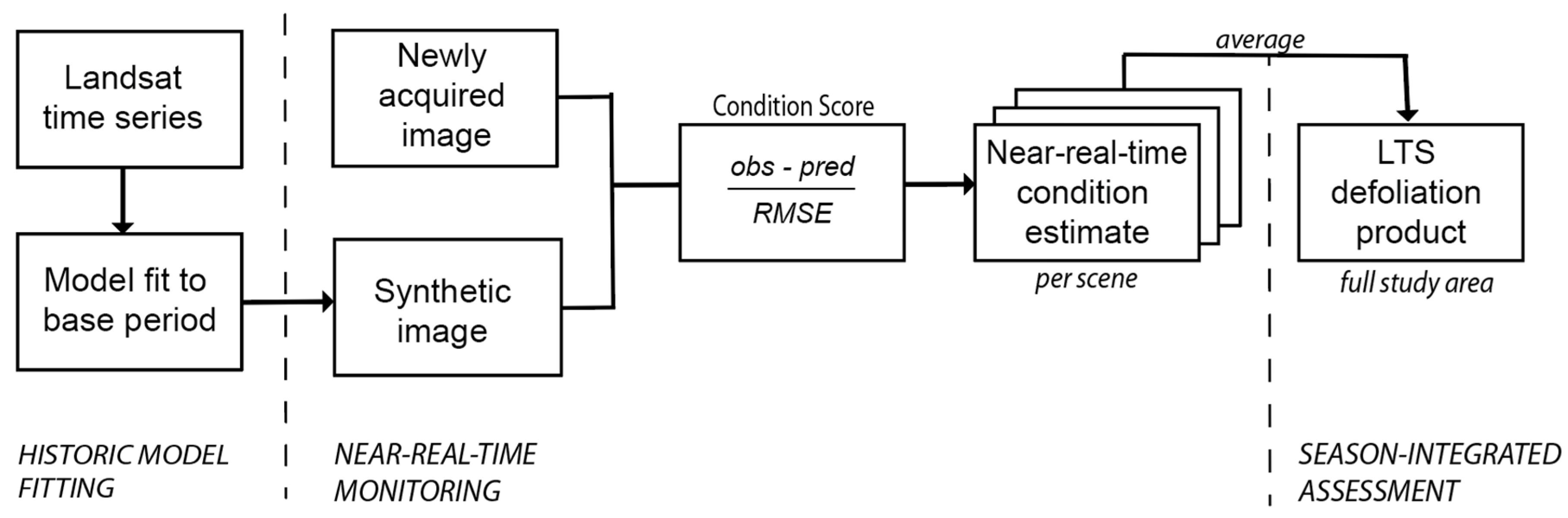
Figure 2.
Example of Continuous Change Detection and Classification (CCDC) model fitting and prediction for a single pixel. The dark gray area shows the stable base period used to generate the CCDC fit model (solid line). The fitted model is used to predict Tasseled Cap Greenness (TCG) values during the monitoring period (in this case, 2016, dotted line). This pixel represents an example of defoliated forest, where observed TCG values from June through August 2016 (green points) were less than half of their modeled long-term average values.

Figure 3.
Examples of near-real-time condition assessments for the area around the Connecticut River Valley in 2016. White areas represent no data due to clouds and cloud shadows. Though each individual assessment may be subject to data loss, changes in condition that are not present in the 2 June image clearly manifest in the 18 June image and persist in the 26 June image. Thus, individual assessments can be considered for rapid response, while use of the temporal domain provides increased certainty that the observed patterns are due to defoliator activity.

Figure 4.
2016 Landsat Time Series (LTS) integrated condition assessment, mid-June through September 2016 for Southern New England. Forest condition in blue areas did not differ from predicted values, whereas darker reds indicate increasing deviation from the 2005–2015 forest condition. Non-forested areas based on NLCD 2011 are shown in black and water bodies appear as white.
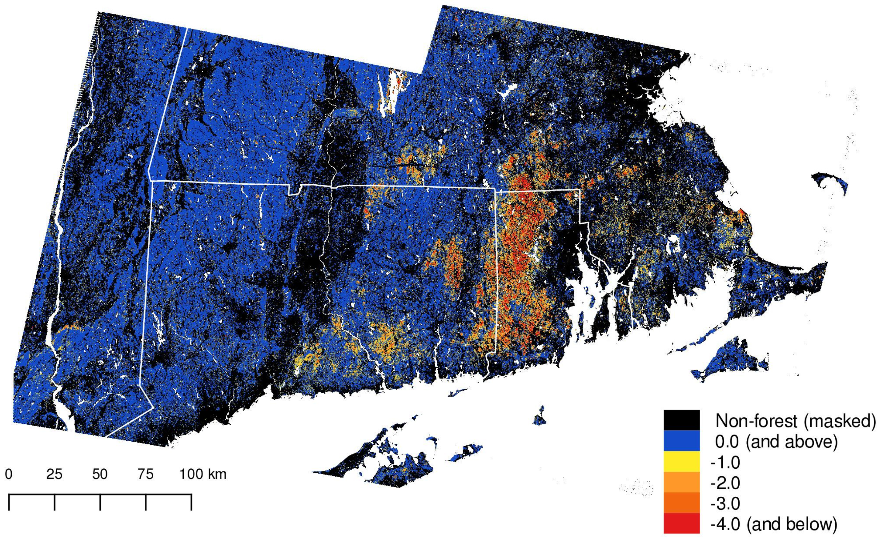
Figure 5.
Histograms showing distribution of Landsat Time Series (LTS) condition scores relative to two other defoliation assessments of forested areas in Southern New England in 2016: (a) aerial sketch maps (provided by USFS regional office), and (b) a remote sensing-based Forest Health Technology Enterprise (FHTET) assessment. Histograms in red tones indicate distributions for areas assessed as defoliated during the 2016 gypsy moth outbreak, while the blue line shows the distribution of scores outside of defoliated areas. The aerial sketch histogram includes four levels of defoliation, while the FHTET histogram shows distributions for three different products: raw results and two post-processed maps where sieving was used to remove isolated pixels. Dotted lines indicate the range between −1.0 and 1.0, assumed to represent little to no damage.

Figure 6.
Map-based comparison of LTS product with other defoliation products describing defoliation from gypsy moths in Southern New England in 2016. Map (a) shows a subset of the LTS map shown in Figure 3; in map (b), the aerial sketch polygons are overlaid on the LTS map; and in map (c), the FHTET product is overlaid on the LTS map. Areas labeled as defoliated in each product are transparent in order to highlight corresponding LTS condition scores, while non-defoliated areas are masked in translucent white. These maps provide a spatial perspective on the distribution of LTS scores shown in Figure 5.
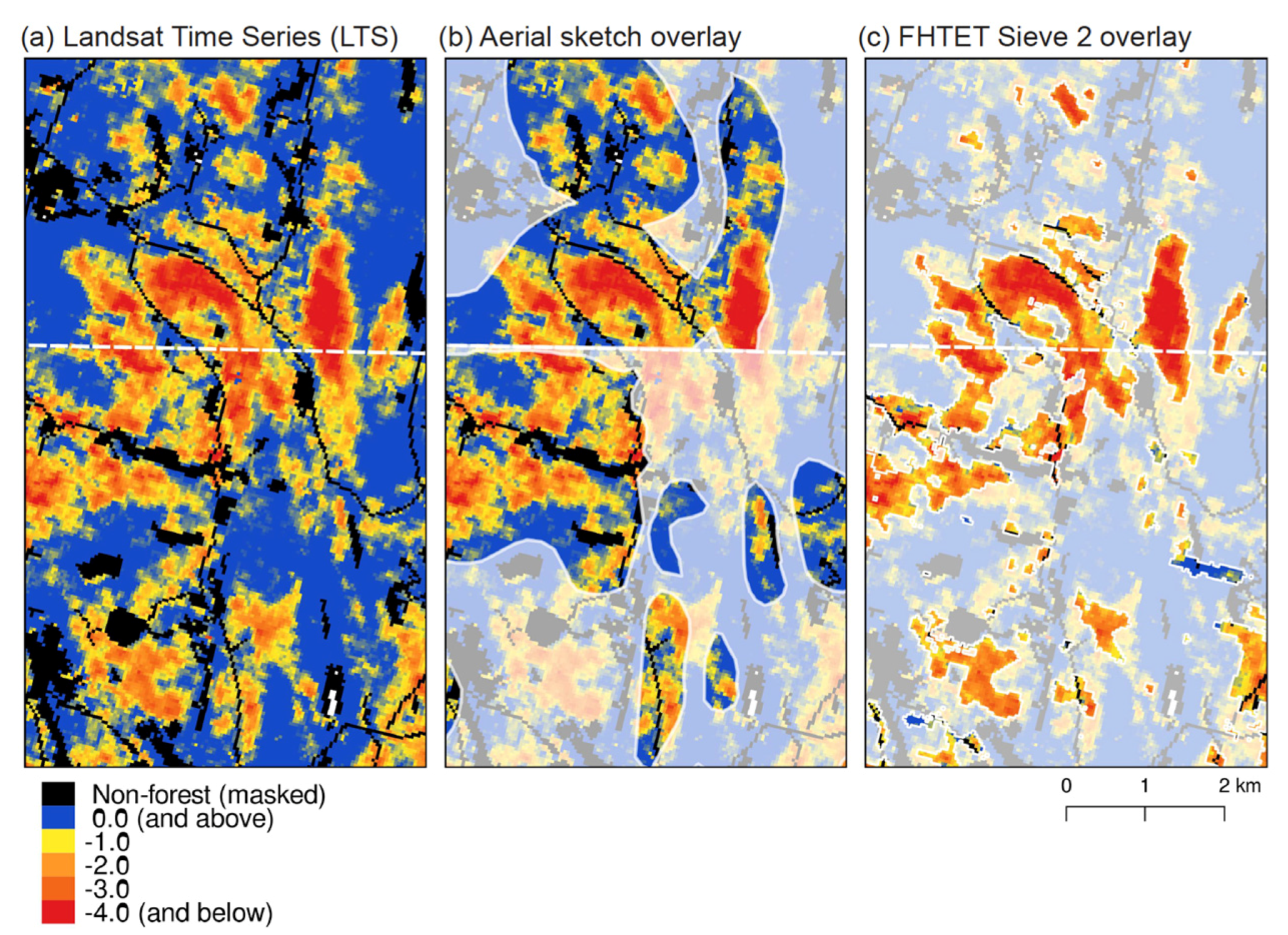
Figure 7.
Map-based comparison of 2016 defoliation estimates for Rhode Island, USA. (a) The LTS product captures fine resolution patterns of damage and provides a metric of defoliation magnitude; (b) The aerial sketch map is coarse resolution, but provides a metric of defoliation magnitude; (c) The FHTET product is fine resolution, but does not provide a metric of defoliation magnitude.


Table 1.
Image dates used in 2016 gypsy moth defoliation analysis.
| WRS-2 | DOY | Date |
|---|---|---|
| 12/31 | 2016-171 | 19 June |
| 12/31 | 2016-179 | 27 June |
| 12/31 | 2016-195 | 13 July |
| 12/31 | 2016-203 | 21 July |
| 12/31 | 2016-227 | 14 August |
| 12/31 | 2016-235 | 22 August |
| 12/31 | 2016-243 | 30 August |
| 13/31 | 2016-170 | 18 June |
| 13/31 | 2016-178 | 26 June |
| 13/31 | 2016-186 | 4 July |
| 13/31 | 2016-194 | 12 July |
| 13/31 | 2016-202 | 20 July |
| 13/31 | 2016-218 | 5 August |
| 13/31 | 2016-242 | 29 August |
| 13/31 | 2016-258 | 14 September |
| 13/31 | 2016-266 | 22 September |
Table 2.
Comparison of defoliation area estimates for Rhode Island, USA, June through September 2016 using Landsat Time Series (LTS) condition scores, remote sensing-based Forest Health Technology Enterprise (FHTET) product, and USFS aerial sketch maps.
Table 2.
Comparison of defoliation area estimates for Rhode Island, USA, June through September 2016 using Landsat Time Series (LTS) condition scores, remote sensing-based Forest Health Technology Enterprise (FHTET) product, and USFS aerial sketch maps.
| Dataset | Area Affected | Percent of RI Forest 1 |
|---|---|---|
| LTS (condition score < −1) | 618 km2 | 49.3% |
| LTS (condition score < −2) | 387 km2 | 30.9% |
| LTS (condition score < −3) | 220 km2 | 17.6% |
| FHTET (Sieve 2) | 641 km2 | 51.2% |
| Aerial (>50% defoliation, Level 5) | 448 km2 | 35.8% |
| Aerial (>30% defoliation, Levels 4, 5) | 520 km2 | 41.5% |
| Aerial (>11% defoliation, Levels 3, 4, 5) | 525 km2 | 41.9% |
1 Total forested area of RI based on NLCD 2011: 1253 km2.
© 2017 by the authors. Licensee MDPI, Basel, Switzerland. This article is an open access article distributed under the terms and conditions of the Creative Commons Attribution (CC BY) license (http://creativecommons.org/licenses/by/4.0/).
Share and Cite
MDPI and ACS Style
Pasquarella, V.J.; Bradley, B.A.; Woodcock, C.E. Near-Real-Time Monitoring of Insect Defoliation Using Landsat Time Series. Forests 2017, 8, 275. https://doi.org/10.3390/f8080275
AMA Style
Pasquarella VJ, Bradley BA, Woodcock CE. Near-Real-Time Monitoring of Insect Defoliation Using Landsat Time Series. Forests. 2017; 8(8):275. https://doi.org/10.3390/f8080275
Chicago/Turabian StylePasquarella, Valerie J., Bethany A. Bradley, and Curtis E. Woodcock. 2017. "Near-Real-Time Monitoring of Insect Defoliation Using Landsat Time Series" Forests 8, no. 8: 275. https://doi.org/10.3390/f8080275
Note that from the first issue of 2016, this journal uses article numbers instead of page numbers. See further details here.