Article

Environmental Factors Driving the Recovery of Bay Laurels from Phytophthora ramorum Infections: An Application of Numerical Ecology to Citizen Science

1
Department of Agricultural, Forest and Food Sciences, University of Torino, Largo P. Braccini 2, I-10095 Grugliasco, Italy
2
Department of Environmental Science, Policy and Management, University of California at Berkeley, 151 Hilgard Hall, Berkeley, CA 94720, USA
*
Author to whom correspondence should be addressed.
Forests 2017, 8(8), 293; https://doi.org/10.3390/f8080293
Submission received: 24 July 2017 / Revised: 8 August 2017 / Accepted: 10 August 2017 / Published: 13 August 2017
(This article belongs to the Special Issue Forest Pathology and Plant Health)

Abstract

:
Phytophthora ramorum is an alien and invasive plant pathogen threatening forest ecosystems in Western North America, where it can cause both lethal and non-lethal diseases. While the mechanisms underlying the establishment and spread of P. ramorum have been elucidated, this is the first attempt to investigate the environmental factors driving the recovery of bay laurel, the main transmissive host of the pathogen. Based on a large dataset gathered from a citizen science program, an algorithm was designed, tested, and run to detect and geolocate recovered trees. Approximately 32% of infected bay laurels recovered in the time period between 2005 and 2015. Monte Carlo simulations pointed out the robustness of such estimates, and the algorithm achieved an 85% average rate of correct classification. The association between recovery and climatic, topographic, and ecological factors was assessed through a numerical ecology approach mostly based on binary logistic regressions. Significant (p < 0.05) coefficients and the information criteria of the models showed that the probability of bay laurel recovery increases in association with high temperatures and low precipitation levels, mostly in flat areas. Results suggest that aridity might be a key driver boosting the recovery of bay laurels from P. ramorum infections.

1. Introduction

The “disease triangle” model [1,2] frames pathogenesis as a process relying on the trophic interconnection between susceptible hosts and pathogens, provided that the environmental conditions are conducive to infection by the pathogen and to disease progression. The interest of forest pathologists in unraveling environmental factors driving plant diseases has been amplified in the last decades by the onset of relevant epidemics caused by emerging pathogens such as Phytophthora ramorum Werres, De Cock and Man in’t Veld in Western North America, Heterobasidion irregulare Garbelotto and Otrosina, Hymenoscyphus fraxineus (T. Kowalski) Baral, Queloz and Hosoya, and Gnomoniopsis castaneae G. Tamietti in Europe, just to cite a few relevant examples [3,4,5,6,7,8,9,10,11,12]. The main environmental drivers underlying the success of such novel epidemics have often been identified through a numerical ecology approach, based on computational and multivariate statistical techniques suitable to deal with complex ecological datasets [10,11,13,14,15,16,17,18,19,20,21,22].
Although environmental factors play a key role in boosting plant diseases, they may also unbalance the interaction between pathogen and host, favoring the latter and promoting recovery of the host. Recovery is not only a theoretical possibility, since it has been extensively documented for a broad range of plant diseases [23,24,25,26,27,28]. However, few studies have proposed a reverse approach to the “disease triangle” paradigm in forest ecosystems, investigating the association between environmental factors and the actual or potential recovery from infectious diseases [29,30,31].
As mentioned above, the invasion by the oomycete P. ramorum has led to one of the most disruptive epidemics in forest ecosystems of North America, especially in California and Oregon [32]. Depending on the host, different diseases displaying a wide range of symptoms have been reported for the same pathogen [33,34,35,36,37,38]. The most relevant among such diseases is “sudden oak death” (SOD), a rapid and severe decline associated with stem bleeding cankers and high mortality rates of Quercus spp. (section Lobatae) and tanoak (Notholithocarpus densiflorus (Hook. & Arn.) Manos, Cannon and S.H. Oh). “Ramorum leaf blight” is instead a foliar disease caused by P. ramorum on bay laurels (Umbellularia californica (Hook. and Arn.) Nutt.), Camellia spp., Kalmia spp. and Rhododendron spp., whose main symptoms are leaves spots, stains and diffuse necroses, as well as browning or blackening, followed by premature leaf fall. Although bay laurels are highly susceptible, they generally display only moderate or mild symptoms, playing a key role as reservoirs of P. ramorum inoculum [39]. However, bay laurels support maximum sporulation levels, while the contribution of tanoaks and oaks in this sense is notably less relevant [40]. Interestingly, P. ramorum is characterized by unusual biological traits within the genus Phytophthora, being a pathogen on aerial parts of the infected hosts, where it differentiates deciduous sporangia acting as the main infective inoculum [38,41]. Once mobilized and aerially spread during rainfalls, sporangia release the zoospores, whose motility in water or wet surfaces facilitates the infection of new hosts [40,41]. Because of its high pathogenicity, spread potential and invasiveness, P. ramorum is considered a serious threat for forests ecosystems in Western North America. Moreover, the pathogen has been sporadically reported in Europe, where it was included by the European and Mediterranean Plant Protection Organization (EPPO) in the A2 list of alien organisms recommended for regulation [35].
Most studies investigating the ecology of P. ramorum agree on the overall conclusion that the pathogen spread is boosted by increasing host densities and high rainfalls levels, while it is hindered by aridity [32,42,43,44,45,46,47]. An innovative approach based on citizen science was recently designed, tested and applied to predict the infection risk by P. ramorum in California and southern Oregon [17,48]. From 2005 to 2015, during the so called “SOD blitzes”, volunteer citizens were engaged to survey forests and urban parks, where they collected soil, water and tree samples geolocated with amatorial GPS devices. Samples coordinates were stored in a geodatabase along with the results provided by laboratory analyses confirming, or not, the presence of P. ramorum. As a result, maps of the current distribution of P. ramorum, as well as estimates of infection risk as a function of latitude and longitude were obtained and integrated in user friendly applications for computers and mobile devices (i.e., “SODmap” and “SODmap Mobile”) [17,48].
Although citizen science has disclosed an interesting potential to support applied environmental research [49,50,51], the appealing possibility of a cost-efficient realization of huge datasets is not risk-free. In fact, the poor scientific background of most citizens along with constraints related to equipment availability may lead to procedural errors, biases an inaccuracy potentially affecting data quality [17,49,50]. For instance, during the “SOD blitzes” [17,48], citizens were not expected to own professional GPS devices. Amatorial GPS are widespread, since they are often integrated by default in popular smartphones, but their error in collecting the right location may vary from a tenth to some hundred meters [52]. Hence, the possibility that some trees were inadvertently resampled in different “SOD blitzes” is likely. Despite being an unsought bias, resampling could be turned into an interesting opportunity allowing the follow-up of the infection by P. ramorum in the same trees, along with the detection of trees whose infection status switched from positive to negative (i.e., recovered trees).
Under the above premise, the main goals of this work were (I) to design and test a general method for the identification and geolocation of the recovered trees, based on a citizen science dataset; (II) to apply the above method to the “SODmap” database; and (III) to test the association between the probability of recovery from P. ramorum infections in bay laurel and some climatic, topographic and ecological factors.

2. Materials and Methods

2.1. Samplings and Laboratory Analyses

Samplings and laboratory analyses leading to the realization of the “SODmap” database were performed within the “SOD Blitz” program, whose details were previously published [17]. From 2005 to 2015 volunteer citizens were recruited to collect water, soil or plant tissue samples. In this study, only the latter were considered to investigate host recovery. Specific training was offered to all volunteers in order to properly detect disease symptoms and standardize sampling procedures. The distribution area of P. ramorum in California and Southern Oregon was systematically monitored and random samplings were carried out in forests sites, urban parks and private gardens. Storage packets were provided to the volunteers for sampling preservation prior to laboratory analyses. The detection of P. ramorum in host-plant tissues was carried out using a species-specific molecular assay previously described [53]. Such assay is based on a highly efficient polymerase chain reaction (PCR) using a 5′ fluorogenic exonuclease (TaqMan) chemistry that combines two species specific primers (Pram5 and Pram6) to an internal probe (Pram6), allowing the detection of target DNA up to a minimum threshold of 15 fg [53]. When the assay detected the presence of P. ramorum DNA, the infection status of the corresponding sample was scored as 1, otherwise as 0. Sampling time, trees species, coordinates and infection status were included in the “SODmap” database.

2.2. Design of the Algoritm to Detect and Geolocate the Recovered Trees

2.2.1. Rationale

Let T = { T 1 , T 2 , T 3 . T K } be a set of K points (i.e., sampled trees locations) whose Cartesian coordinates xT and yT (m) are exact, but unknown. T is composed by the sets V = { V 1 , V 2 , V 3 . V N } and W = { W 1 , W 2 , W 3 . W M } including N and M trees, respectively, with N + M = K , V W = T and V W = . Trees coordinates for sets V (xV, yV) and W (xW, yW) are estimated with a GPS device whose median value ε of the radial error r (m) is known [54]. Coordinates collection is performed once for V set (i.e., single-sampled trees), and more than once for the W set (i.e., resampled trees). Hence, the set V = { V 1 , V 2 , V 3 . V N } , derived from V, includes N trees with estimated coordinates xV’ and yV’. Similarly, the set W = { W 1 , W 2 , W 3 . W M } is gathered from W and includes M’ > M trees with coordinates xW’ and yW’. Let T = V W = { T 1 , T 2 , T 3 . T K } be a set of K’ points with coordinates xT’ and yT’. All elements of T’ are in bijective association with K’ elements of the set I = { I 1 , I 2 , I 3 . I K } , expressing the infection status (i.e., if positive to the pathogen 1, else 0), and with K’ elements of the set S = { S 1 , S 2 , S 3 . S K } , indicating the sampling time. Under this premise, a citizen science dataset includes T’, I, S with the corresponding GPS coordinates xT’ and yT’, while the partitioning of trees locations between the sets V and W is unknown.
Let Φ Λ be an algorithm operating as a binary classifier based on partitioning [55] and able to split T’ into the two mutually exclusive sets W ˜ and V ˜ , estimates of W’ and V’, respectively. The partitioning mechanism is based on the application of a virtual squared grid over the point features representing the T’ trees. A grid-system cannot discriminate distinct points locations if their distance is below its spatial resolution, which is determined by the length of the grid-cells edge (i.e., pixel size). Such points are merged by the grid-system, as if they were not spatially distinct [56]. However, the separation observed among some point features (i.e., W’) can be an artifact deriving from the iterated estimation of the same locations (i.e., W) with a GPS device affected by some spatial location error. Hence, Φ Λ can classify such points as deriving from accidental resampling (i.e., W ˜ ) through a grid-based system Λ ϑ with adequate spatial resolution ϑ . Φ Λ assigns to the set W ˜ the neighboring points features falling into the same pixel, since they cannot be resolved by the spatial resolution of Λ ϑ (Figure 1). The set W ˜ is derived from W ˜ by averaging its points coordinates at pixel level, while the other points are then classified as V ˜ elements. Finally, the set of recovered trees R = { R 1 , R 2 , R 3 } is identified by Φ Λ as the subset of W ˜ whose infection status switched from 1 to 0, from the first to the last sampling.

2.2.2. Modelling GPS Error and Spatial Resolution of the Grid-System

The Φ Λ algorithm is based on the selection of an adequate spatial resolution ϑ which is dependent upon the GPS error scattering the resampled trees features (i.e., W’) around their true location (i.e., W). The mathematical structure of the GPS error was modeled prior to its relation with the spatial resolution of the grid-system.
The Rayleigh distribution f ( r | σ ) = r σ 2 e r 2 2 σ 2 parametrized by σ and with median value E = σ 2 l n 2 was assumed as the probability distribution function (PDF) of r [54,57]. The goodness-of-fit of the Rayleigh PDF to r was experimentally tested with an in-field trial. In January 2017, a point location with known coordinates (389,095.5 m, 4,990,997.5 m, UTM WGS 1984 zone 32N, EPSG 32632) was identified in an open space flat area of Western North Italy. The point coordinates were collected 200 times in different days and daylight hours with a professional GPS device (Magellan MobileMapper 6), resulting in 200 point location estimates (Dataset S1). The GPS radial error r was calculated for each point location estimate as the Euclidean distance separating the true coordinates from the assessed ones [54]. The adequacy of the Rayleigh PDF to model r was tested with the Kolmogorov-Smirnov goodness-of-fit test [58], parametrizing the Rayleigh curve with the maximum likelihood estimate of σ [57].
A functional relation ϑ = f ( ε ) was assessed in silico with Monte Carlo (MC) methods to allow the selection of ϑ from ε, which is a parameter associated with the GPS device [52]. A set of 103 GPS coordinates collection of a known virtual tree location was simulated 103 times for each integer value of ε included between 1 and 3 × 10³. The GPS location error was randomly sampled from a Rayleigh PDF. The maximum pairwise distance obtained for each set of GPS coordinates was set as ϑ value. After a visual examination of the scatterplot displaying the ε and the associated ϑ values, a linear regression model with no intercept was fit. Its performances were assessed in terms of ε coefficient (βε) significance, minimum Akaike information criterion (AIC) and maximum AIC weight (AICw), setting as reference baseline the null model [58,59,60]. Details about the algorithm performing the MC simulations are reported in Note S1.
Once ϑ is defined based on ε, Λ ϑ can be integrated as a sliding grid-system into Φ Λ to provide different alternative scenarios estimating R. Such alternatives account for different possible positions of the grid-system.

2.2.3. Design of the Algorithm

The algorithm was designed in R language as a two-step process consisting in distinct blocks of code embedded into specific R-functions [58]. The first block, starting from the trees coordinates xT’ and yT’ and from the median value ε* of the GPS radial error, builds up the virtual grid-system Λ ϑ by fixing its spatial extent and spatial resolution ϑ . The grid layer is located over the map of the study area including all trees locations and randomly fixing the coordinates of its left-bottom corner. Trees whose location cannot be resolved based on ϑ are sent to the second block of code ( Φ Λ ) . The latter processes the sampling year and the infection status for each cell, detecting trees sampled in different years and selecting the ones whose infection status switched from 1 to 0 (i.e., recovered trees R). Since the classifier Φ Λ includes Λ ϑ as a stochastic component (i.e., the left-bottom vertex coordinates of the grid), alternative scenarios estimating R are possible. Their assessment can be achieved by embedding Λ ϑ as a sliding grid-system into Φ Λ through iterate runs of the two algorithm blocks (i.e., loop [58]). Technical details about the algorithm design are included in Note S2.

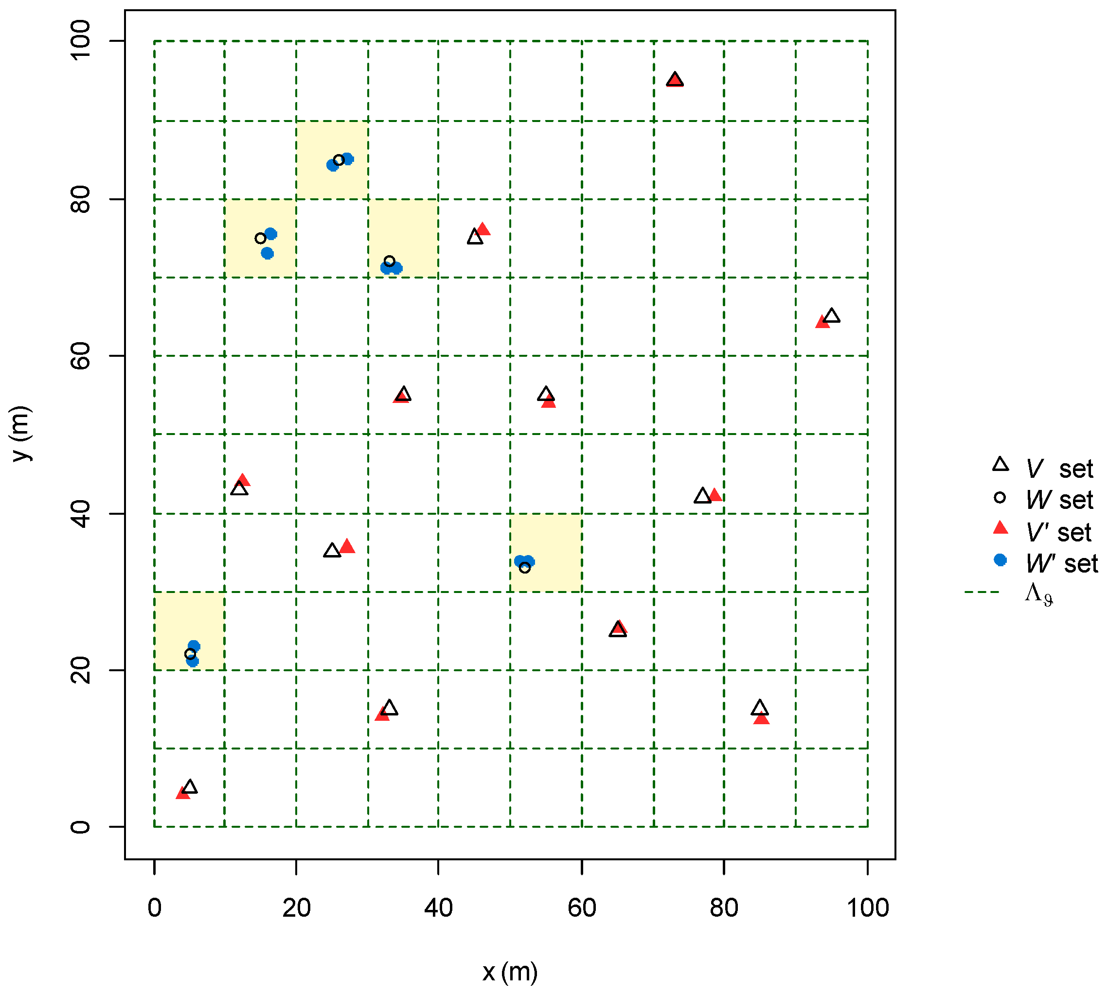
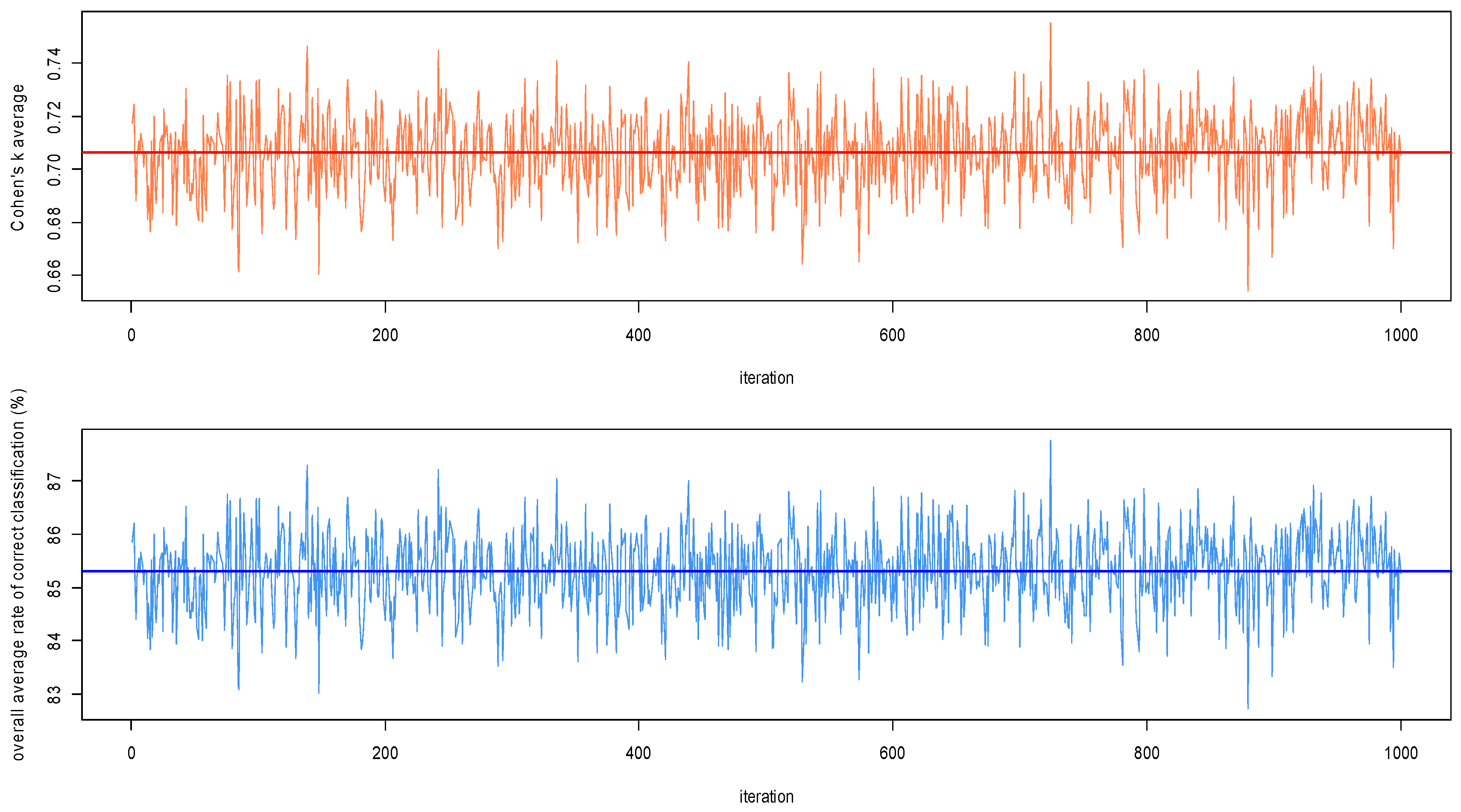
2.2.4. Algorithm Performances Assessment

Algorithm performances were assessed in silico with a series of MC simulations [61]. In a virtual squared area extended for 104 km2, the sets V’ with N = 200 and W with M = 100 were simulated by randomly extracting the associated coordinates xV’, yV’, xW and yW from a uniform distribution [57] limited between 0 and 100 km. A constant infection status and sampling year was assigned to the elements of V’. A virtual GPS with median radial error ε* = 100 m was used to mimic the process of coordinates collection on W, setting two samplings for each element in W, and resulting in M’ = 200 estimated trees locations included in the set W’. The radial error r of every virtual GPS coordinates collection was randomly extracted from a Rayleigh distribution whose parameter σ was calculated by solving the equation E = ε* [57]. Each element of W was then associated with the couple of related elements in W’. Random consecutive sampling years were assigned to the above couples. One of the four permutations of the infection status was randomly assigned to each fourth of the couples.
Φ Λ was applied to the set of trees locations based on 103 different random positions of the sliding grid-system Λ ϑ . The ability of Φ Λ in partitioning the trees between W’ and V’ was assessed with the Cohen’s k statistics and overall rate of correct classification (%) [62,63,64], which were averaged within all 103 positions of Λ ϑ . The above MC simulation was iterated 103 times.

2.3. Detection and Geolocation of the Trees Recovered from P. ramorum Infections Based on the “SODmap” Database

Only the input needed by the Φ Λ algorithm was retained from the original “SODmap” database, which was filtered to remove all unnecessary information [17,48]. Sampled trees coordinates were reprojected into UTM NAD83 zone 11N (EPSG 4326) and included within a polygon shapefile in a GIS environment [65].
Assuming that trees coordinates had been collected by volunteers endowed with GPS sensors embedded in smartphones, iPhones or comparable devices [17,48], two scenarios were analyzed depending on the GPS median radial error ε*. Based on thresholds reported in previous studies [52], the minimum and maximum ε* were set to 10 m and 500 m, respectively, defining two alternative scenarios (i.e., scenario-10 m and scenario-500 m). For both scenarios, the detection and geolocation of trees recovered from P. ramorum infections were performed by applying Φ Λ , with 103 iterations, accounting for different locations of the grid-system. The algorithm was run separately for bay laurel, tanoak and oaks, allowing reproducibility by fixing a unique seed number to each run (provided in Dataset S2). The output datasets were ranked within host species and scenarios depending on the number of elements included in the set W ˜ at each iteration. Datasets displaying the maximum number of elements were selected for further analyses. If several of the above datasets resulted from the same tree species and scenario (i.e., alternative datasets), they were tested for equivalence based on the comparison of their associated two-dimensional Gaussian kernel density estimate (KDE) matrices [58,66,67]. KDE matrices and their associated rasters were obtained by setting a common bandwidth [67] and the cells edge to 10 km, with extension and resolution allowing for a perfect cell-wise alignment. Comparisons among KDE matrices were performed with the Kruskal-Wallis or Mann-Whitney tests for the mean and with the Fligner-Killeen test on rank-transformed data for the variance [58,68]. Since some alternative datasets were equivalent (see Results), a random selection of the final datasets to include in the further analyses was performed. The number of resampled trees included in W ˜ for each scenario and host species was calculated and compared to the corresponding number of trees from the screened “SODmap” dataset. Similarly, the incidence of trees recovered from P. ramorum infections was calculated as absolute count and in percent. The latter, including 95% confidence intervals, derived from ratio between the recovered trees and the trees which have been infected at least once [69].

2.4. Analysis of the Association between Environmental Factors and Recovery from P. ramorum Infections

Because of the low number of oaks and tanoaks recovered from P. ramorum infections (see Results), the association between recovery and environmental factors was tested only for bay laurels. The averages of the minimum, maximum and mean temperatures (Tmin, Tmax, Tmean, °C) and cumulate precipitations (P, mm) were calculated at pixel level based on the yearly values of the rasters derived from parameter-elevation regressions on independent slopes models (PRISM-4 km) in the period 2005–2015 [70,71]. Elevation (El, m) rasters were obtained from digital elevation models (DEM) provided by the NASA Shuttle Radar Topographic Mission in the 30 arc-sec (~900 m) version (SRTM30) [56,72]. Estimates of bay laurel density (Bld, trees/ha) were gathered from an available source raster [73]. All rasters were reprojected into UTM NAD83 zone 11N (EPSG 4326) and cropped within the borders of the study area. Aspect (As, as azimuth, °), slope (Sl, %), terrain ruggedness (as Terrain Ruggedness Index—TRI [74]), topographic position (as Topographic Position Index—TPI [75]) were derived from GIS geomorphological analyses carried out on the DEM [76]. All rasters were converted into matrices [58], whose basic descriptive statistics (range, average, coefficient of variation (CV)) were calculated, with the exception of As. The Bld raster was trimmed discarding pixels below 150 and above 1500 to improve analyses robustness [77].
The associations between recovery from P. ramorum infections and Tmin, Tmax, Tmean, P (i.e., climatic factors) El, Sl, TRI, TPI (i.e., topographic factors), and Bld (i.e., ecological factor) were tested through a numerical ecology approach based on correlation analyses and binary logistic regressions [58,63]. For both scenarios, the binary dependent variable was coded as 1 for recovered trees, as 0 for the other trees whose infection status to P. ramorum had been positive at least once. The continuous predictors were obtained by extracting from the rasters of the environmental factors the cell values corresponding to each tree location. In addition, trees latitude (Lat) and longitude (Long) in UTM NAD83 zone 11N (EPSG 4326) were included as predictors. Colinearity among predictors, except As and Bld (see below), was tested by calculating all possible pairwise Spearman’s ρ coefficients and results were visualized through circular correlograms [58]. Binary logistic regressions were fitted with single and multiple predictors, including the intercept (β0). Combinations of multiple predictors were included only in the absence of significant pairwise correlations [61,63]. All models within the same scenario were compared in terms of sign and significance of the predictor coefficient (β), range of its associated 95% CI, minimum AIC and maximum AICw, setting the null model as reference [58,59,60,63].
The robustness of the results obtained from binary logistic regression models was assessed through a MC simulation trial [61] accounting for a putative overall misclassification rate associated with Φ Λ . Since the Φ Λ algorithm displayed an average overall rate of correct classification theoretically attaining 85.3% (see Results), the putative misclassification rate was set to 15%. Hence, all binary logistic regression models were run on a dependent variable whose 15% of values was randomly selected and reverted at each iteration, until 105 iterations were conducted. From the resulting β coefficients distributions, the associated 95% CI were calculated (i.e., MC 95% CI) [78] and the bound signs were compared with the corresponding 95% CI obtained from the fit on the original dataset.
Bay laurel density models were fitted only as single predictor models and excluded from the comparative assessment with the others because of missing data. As was not included as predictor because of data circularity [79]. Hence, azimuth distributions were compared between recovered and not recovered bay laurels with the Mardia-Watson-Wheeler test and the Rao’s homogeneity test [80,81]. A complementary correlation and partial correlation analysis was carried out between KDE matrices of recovered trees and matrices of Tmin, Tmax, Tmean, P, El, Sl, TRI, TPI, and Bld (Note S3).

2.5. Software and Libraries Used for Statistical, GIS and Numerical Analyses

Statistical and numerical analyses were run in R version 3.2.3. with libraries binGroup, circular, extraDistr, Hmisc, igraph, maptools, MASS, MuMIn, ppcor, psych, raster, rasterVis, REdaS, spaa, spatstat. GIS data manipulation and related analyses were performed both in R and in QGIS 2.8.5-Wien. All statistical tests were carried out with a cut-off significance threshold set to 0.05.

3. Results

3.1. Design of the Algorithm to Detect and Geolocate the Recovered Trees

3.1.1. GPS Error and Spatial Resolution of the Grid-System

The 200 GPS radial errors r ranged between 0.07 m and 4.52 m, with an average of 1.64 m. The maximum likelihood estimate of σ attained 1.32 m and the resulting Kolmogorov-Smirnov test was non-significant (p = 0.553) confirming the adequacy of the Rayleigh PDF to model r.
The MC experiment produced a total of 3 × 10⁹ GPS estimates of the single tree location, split in 103 assessments of 103 independent sets of points for each of the 3 × 10³ values of the GPS median radial error ε (Figure S1). The linear regression model displayed a significant coefficient βε = 6.033 (p < 0.05) and outperformed the null model for all metrics considered (AIC = 47457202, vs. AIC = 59928055 and AICw = 1 vs. AICw = 0). Hence, the functional relation ϑ = f ( ε ) was assessed as ϑ = 6.033 ε .

3.1.2. Design of the Algorithm

The first block of code resulted in a 32 lines script in R language embedded in the function LAMBDA(x, y, theta), which defines the grid-based system Λ ϑ . LAMBDA inputs are the vectors of coordinates x = xT’ and y = yT’, associated with trees in T’, and the t h e t a = ϑ value gathered from the equation ϑ = 6.033 ε (see 3.1.1). LAMBDA output is a vector γ assigned to each element of T’, NA included, identifying with a unique cell-code the locations that cannot be resolved based on ϑ . A map of T’ locations along with the associated grid with spatial resolution ϑ is provided as additional outcome.
The second block of code, defining the classifier Φ Λ , resulted in a 35 lines R-script incorporated into the function PHI(x, y, I, S, gamma). In addition to the coordinates of trees in T’, the function requires input vectors indicating the infection status (I), the sampling time (S) and the γ (gamma) values provided by LAMBDA. PHI output consists of a matrix object with one row per each element of the set W ˜ and five columns indicating the associated “switch-code”, x and y coordinates, the first and the last sampling time, respectively. Column names are returned by the function as switch, xmed, ymed, fy and ly, respectively. “Switch-code” values refer to the transition of infection status from the first to the last sampling, indicated as: “1” from 0 to 0, “2” from 0 to 1, “3” from 1 to 0 (i.e., set R, recovered trees), and “4” from 1 to 1. Functions LAMBDA and PHI are provided as R-scripts in Algorithm S1 and S2 [58].

3.1.3. Algorithm Performances Assessment

A total of 106 runs of Φ Λ resulted in 103 average values of the Cohen’s k statistic and of the overall rate of correct classification, each one based on 103 different positions of the Λ ϑ sliding grid-system. The average Cohen’s k ranged from 0.654 to 0.755, with a global average of 0.706, while the overall rate of correct classification was included between 82.7% and 87.8%, with an overall mean attaining 85.3% (Figure 2). Based on the threshold reported [64] for Cohen’s k, the classification performed by Φ Λ ranks at the 2nd place out of 6 classes, displaying “substantial agreement” between observations (i.e., simulated sets) and predictions (i.e., Φ Λ classifications).

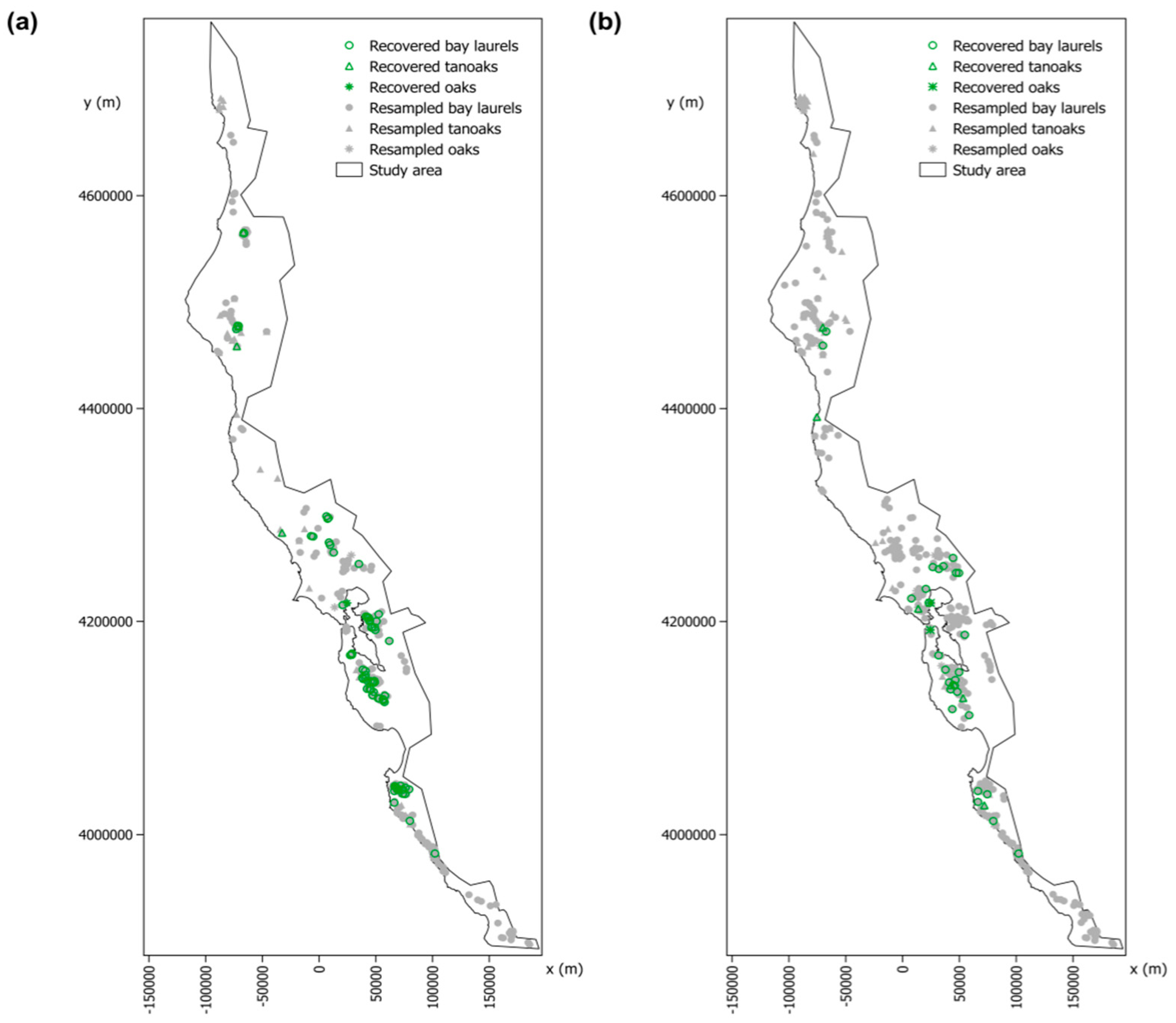
3.2. Detection and Geolocation of Trees Recovered from P. ramorum Infections Based on the “SODmap” Database

The filtering of the original “SODmap” database resulted in a matrix with 19,211 records, one per sampled tree, and 8 fields providing the input for the classification algorithm (Dataset S3). A topographic surface of over 36,700 km2 was delimited within the borders of the study area, with an extension of approximately 920 km along the major axis N-NW/S-SE oriented. Within this area, Φ Λ detected a single dataset for bay laurel and some alternative datasets for oaks and tanoak in both scenarios. Such alternative datasets were equivalent based on the outcomes of the KDE matrices comparisons (see Note S4). Host species final datasets are provided as Datasets S4 and S5 for scenario-10 m and scenario-500 m, respectively.
In the filtered “SODmap” dataset, 14,666 out of 19,211 trees were bay laurels (76.3%), 2468 tanoaks (12.8%) and 157 oaks (0.82%), while the remaining plants (10%) were classified as other host species. In scenario-10 m the algorithm detected 1044 resampled trees ( W ˜ ) including 943 bay laurels (90.3%), 88 tanoaks (8.4%) and 13 oaks (1.2%). Similarly, 284 bay laurels (75.3%), 79 tanoaks (21.0%) and 14 oaks (3.7%) out of 377 resampled trees were detected in scenario-500 m. In percent, resampled trees accounted for 1.96% and 5.43% of the sampled trees in scenario-10 m and scenario-500 m, respectively. The percentage of trees recovered from P. ramorum infections (R) ranged from 9.3 to 32.9% depending on host species and scenario, while the overall percentage was substantially homogeneous between scenarios (29.7% in scenario-10 m and 28.6% in scenario-500 m). Bay laurel attained the largest incidence of recovered trees (approximately 32–33%), followed by oaks and tanoak (Table 1). The distribution of resampled and recovered trees in the study area is shown in Figure 3 for both scenarios.

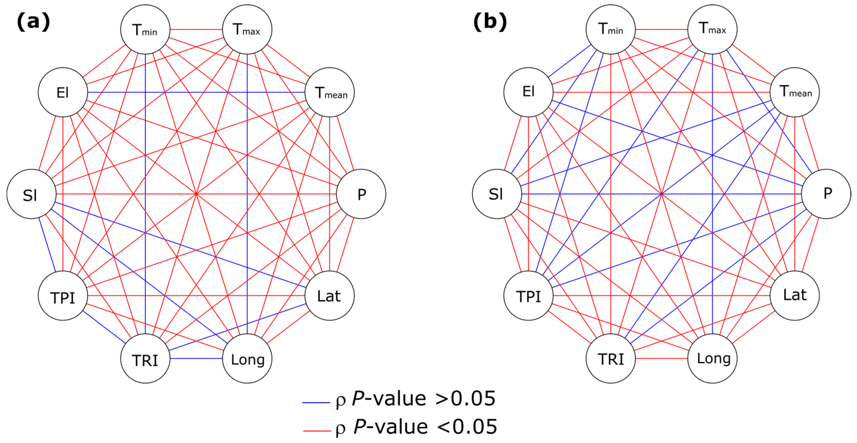
3.3. Analysis of the Association between Environmental Factors and Recovery from P. ramorum Infections

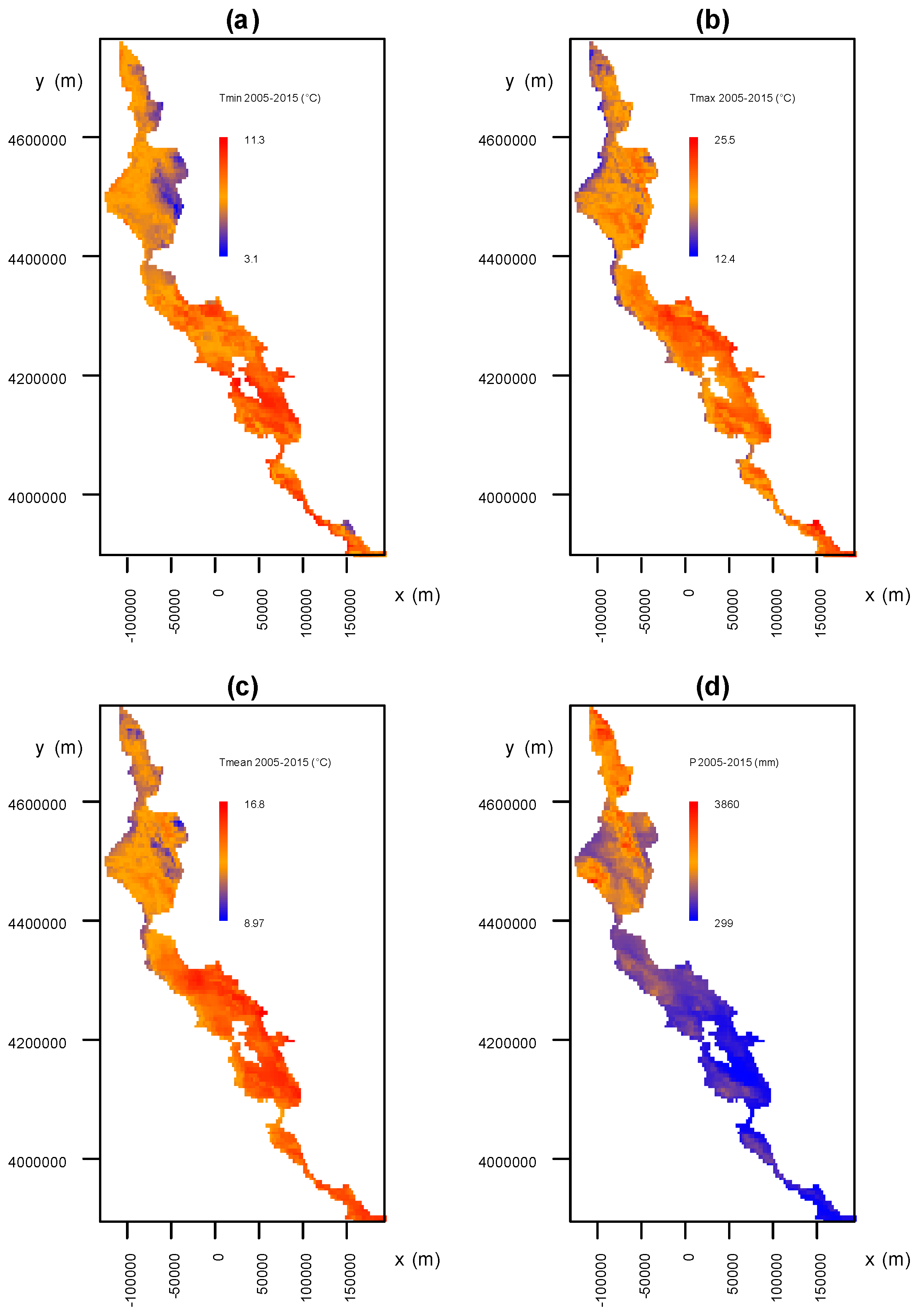
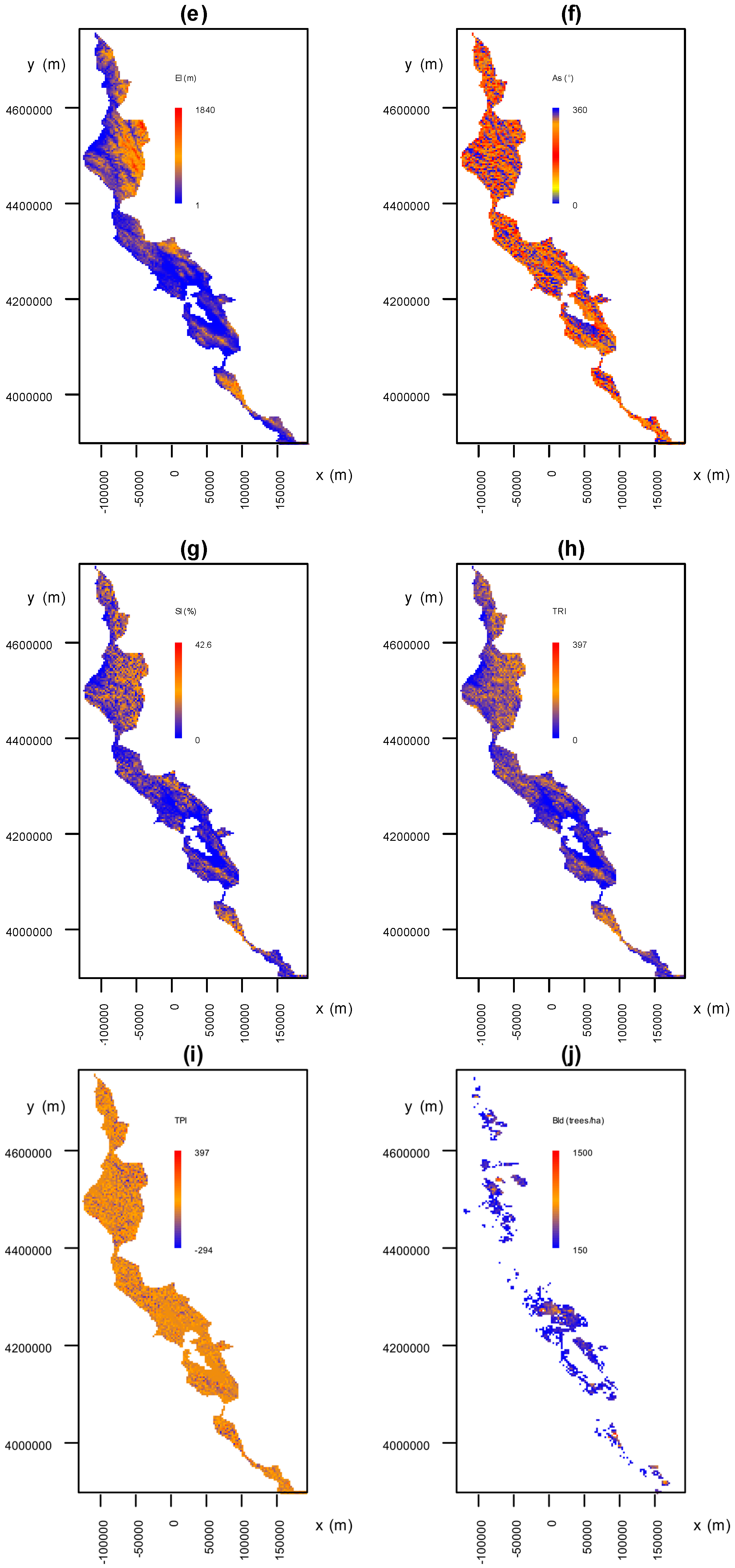
3.3.1. Environmental Factors

A series of 10 derived rasters were obtained for the environmental factors Tmin, Tmax, Tmean, P, El, As, Sl, TRI, TPI, and Bld (Figure 4). All rasters were continuously distributed within the study area with the exception of Bdl, whose patchy covering was due to missing data from the source raster. On average, temperatures during the timeframe 2005–2015 attained 7.62 °C, 19.68 °C, 13.65 °C for Tmin, Tmax and Tmean, respectively, with the highest variability observed for Tmin (CV = 18.69), followed by Tmax (CV = 10.84) and Tmean (CV = 10.40). In the same period, precipitations across the study area were more variable than temperatures (CV = 56.07), with a yearly average of 1236.43 mm. The study area was also characterized by an average El of 375.26 m (CV = 84.36) and a mean Sl value of 8.19% (CV = 74.81), while TRI and TPI attained averages of 80.83 (CV = 61.91) and 0.5 (CV = 12 × 103). Finally, the average value achieved by Bld was 297 trees/ha (CV = 49.92).

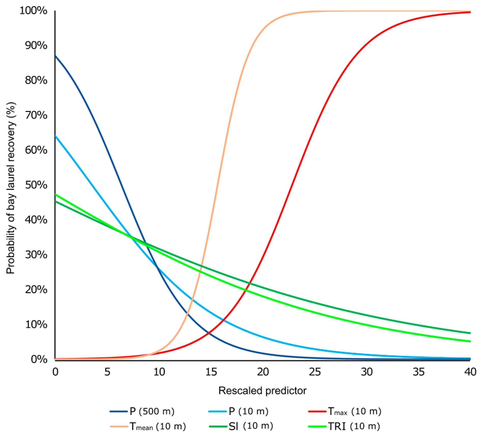
3.3.2. Binary Logistic Regression Models

Correlograms showed that 36 and 32 out of 45 pairwise Spearman’s ρ correlation coefficients between predictors were significant (p < 0.05) in scenario-10 m and scenario-500 m, respectively (Figure 5). Hence, the 9 couples of uncorrelated predictors were included in multiple binary logistic regression models in scenario-10 m. Similarly, multiple binary logistic regressions were fitted on the 13 couples and one triad of uncorrelated predictors in scenario-500 m.
A total of 14 out of 21 and 7 out of 26 binary logistic regression models displayed significant β coefficients (p < 0.05) in scenario-10 m and scenario-500 m, respectively (Table S1). P was significantly (p < 0.05) and negatively (β < 0) associated with the probability of bay laurel recovery in all models where it was included as predictor, namely, one model in scenario-10 m and 7 models in scenario-500m. Such models ranked first based on AIC and AICw, the latter attaining 87.1% in scenario-10m and a cumulative value of 94.4% in scenario-500 m. In all cases, the bounds of the 95% CI associated with P displayed negative lower and upper bounds, hence confirming the results gathered from p-values. The same outcome was observed in MC 95% CI, supporting the robustness of the negative association between P and the probability of bay laurel recovery when assuming a 15% putative misclassification rate in the Φ Λ algorithm. In scenario-500 m, no other climatic and topographic factors displayed either significant β coefficients or 95% CI with lower and upper bounds of the same sign. Accordingly, the signs of the bounds were discordant also in the associated MC 95% CI. However, in comparison to the model with P as single predictor (AICw = 6.8%), the environmental factors Tmax and TPI (with β > 0), TRI and Sl (with β < 0) improved model performances when included in multiple regressions along with P (AICw from 10.4 to 37.5%). In the same scenario, Bld was characterized by a negative β coefficient with a 95% CI excluding 0, but with a p-value > 0.05 and a MC 95% CI with a negative lower bound and a positive upper one. In the other scenario, in addition to P, significance of the β coefficient (p < 0.05) was achieved by Tmax, Tmean (with β > 0), TRI and Sl (with β < 0), indicating that the probability of bay laurel recovery is positively associated with increasing mean and maximum temperatures, but negatively associated with increasing terrain ruggedness and slope. Such associations were confirmed by the concordant signs of the lower and upper bounds displayed by both 95% CI and MC 95% CI. The graphs of the logistic equations modelling the probability of bay laurel recovery based on the single significant predictors detected in the two scenarios are shown in Figure 6. Although in some models Long was positively and significantly associated with the probability of bay laurel recovery (β > 0 and p < 0.05), such association was never confirmed by MC 95% CI, including 0 between the bounds. The remaining predictors were non-significant (p > 0.05) and showed both 95% CI and MC 95% CI with discordant signs, pointing out the lack of association with the probability of bay laurel recovery.

3.3.3. Aspect Analysis

Regardless of the scenario, the azimuth distributions extracted from the As raster (Figure S2) did not display significant differences (p > 0.05) between recovered and not recovered bay laurels (Table 2). The outcomes of Mardia-Watson-Wheeler and Rao’s homogeneity tests were consistent within each scenario.

4. Discussion

Citizen science is an unsurpassable opportunity for basic and applied research, allowing the collection of huge amount of data with a limited financial investment, yet data quality may be questionable as the result of recruiting non-specialized volunteers [49,50,51]. Nonetheless, as shown in our study, some of the errors intrinsic to citizen science datasets might be turned into valuable information, providing new insights into biological and ecological processes, such as plant disease dynamics.
A massive amount of epidemiological data had been gathered from the long-term monitoring (2005–2015) and mapping of the alien invasive plant pathogen Phytophthora ramorum in Western North America, during one of the largest citizen science experiments ever conducted in forest research [17,48]. The resulting “SODmap” database included thousands of records reporting the infection status of each sampled host-tree, along with its estimated coordinates [17,48]. However, such coordinates had not been collected with professional GPS, and trees had not been marked or labeled in the field. Hence, the risk that volunteers had accidentally resampled some of the trees was rather likely. Despite being an unsought side-effect of the data collection process [17,48], resampling turned into an interesting occasion to follow up the infection status in the same trees and detect the ones which had recovered. By reverting the traditional “disease triangle” paradigm, our study was focused on testing the association between recovery from P. ramorum infections in bay laurel and the underlying climatic, topographic and ecological (i.e., environmental) factors through an innovative approach combining numerical ecology to citizen science.
A classification algorithm based on the notion of spatial resolution was designed to extract from the “SODmap” database the “hidden” information about the location of putatively resampled trees [56]. Whenever tree coordinates are repeatedly collected with a GPS device, the resulting location estimates are scattered around the true location as a consequence of the error associated with the GPS [52,54]. If a squared window (i.e., pixel) with suitable spatial resolution is overlapped to such estimates, it cannot spatially resolve them as separate, thus revealing the presence of a single resampled tree location. Basically, the classification algorithm detects resampled trees by incorporating this window as cell of a regular grid, whose spatial resolution is gathered from the GPS median radial location error.
The trials performed in the field with a GPS device, and in silico with Monte Carlo (MC) simulations, confirmed the plausibility of the assumptions underlying the classification algorithm, namely I) that the unknown GPS radial error can be modeled by a Rayleigh probability distribution, and, II) that the spatial resolution of the grid and the median of the above error can be functionally related. Although assuming a spatial homogeneous function to model the GPS radial error might lead to an excessive simplification, especially in mountain areas where the geomorphology could interfere with the GPS signal, the adequacy of the Rayleigh distribution was supported by the outcomes of the Kolmogorov-Smirnov test [57,58]. Moreover, collecting GPS coordinates in different hours of the day, for approximately one month, should have successfully prevented satellite configuration biases potentially influencing the above results. Despite coordinates used for the Kolmogorov-Smirnov test having been collected in Italy, the displacement from the Californian sampling sites seems to be an unlikely source of error in such a long-term trial, especially because the coverage offered by GPS satellites is comparable between Europe and USA. Finally, the functional relation between median GPS radial error and spatial resolution of the grid was clearly shown by the adequacy of the linear regression model fitted on the MC outcomes.
The algorithm performances were satisfactory, as demonstrated by the large overall rate of correct classification (on average over 85%) and by the substantial agreement between the simulated values and the classification outcomes (average Cohen’s k over 0.70) [62,63,64]. However, such performances were not optimal, probably due to the fact that the algorithm classification process is based on a grid with rigid shape and fixed orientation. Once the grid is virtually overlapped on the map of trees locations, it may erroneously split fake locations deriving from the same tree among different pixels. Conversely, the grid might also incorrectly include within the same pixel both resampled and not resampled trees. It is worth noting that, while stem diameters of trees do not reach the meter, the GPS median error and the associated spatial resolution of the grid are in the order of several meters, hence the potential effect of tree size on the classification process should be negligible. Additional sources of misclassification might derive from false-positive or false-negative rates in laboratory assay, yet their occurrence is also unlikely, based on evidence previously published [82]. Finally, misclassification associated with the co-occurrence of localized infections by P. ramorum and sampling of uninfected tissues within the same tree seems quite improbable, since an accurate training about symptoms detection and samples collection was offered to all volunteers [17,48]. Considering that a non-null misclassification rate was somehow predictable, the grid-system was incorporated into the algorithm as a sliding layer, allowing stochastic iterate applications on the same dataset, leading to alternative outcomes [61]. While in simulation trials the best position of the grid can be determined, this is not possible during in-field applications, hence the equivalence/divergence of the outcomes should be assessed based on statistical and geostatistical approaches, depending on the overall aim of the analysis [65]. The same issues would have also arisen if the classification algorithm had been based on continuous probability, rather than on a discrete grid-system. In fact, even assuming that the probability of being a resampled/not resampled tree could be calculated for each GPS location, the assignment to one of the two classes would depend on the selection of an arbitrary probability threshold, ultimately leading to multiple outcomes, as documented for other classification processes [63,83]. Although we recognize that different computational approaches might have been proposed, this study was aimed neither at identifying an optimal theoretical solution, nor at contrasting and ranking alternative classification algorithms. Rather, our major goal was to design and test a single method, whose performances could be adequate for practical applications. Moreover, outcomes of the algorithm are fully reproducible, since the code is released in R, a popular open-source programming language for scientific data analysis [58].
The classification algorithm was run under two alternative scenarios, each one accounting for different levels of GPS precision. The median radial error was set to 10 m and 500 m, respectively, based on the assumption that the most practical way to collect coordinates for citizen scientists was to use the GPS embedded in their smartphone. Such thresholds are consistent with data reported in the literature [52]. Although larger values cannot be excluded [52], the most likely precision of sampling efforts should be around 10 m. In fact, non-specialized volunteers would have easily detected sampling positioning errors in the range of hundreds of meters with any mobile mapping application (e.g., Google Maps, Google Earth, OruxMaps or others) even at a coarse spatial scale. In such cases, coordinates would have been discarded by the volunteers based on the quality control phase of the “SOD blitz” program, a phase performed by the volunteers themselves after data are published on the web [17,48].
Results gathered from the classification algorithm identified only 2–5% accidental resampling rates. Such low percentages lead to a negligible error when modelling the distribution of P. ramorum at statewide scale, further confirming the reliability of the citizen science approach underlying the “SODmap” [17,48]. However, and as an unexpected side benefit, the number of resampled trees provided an adequate sampling size to investigate the probability of recovery, at least for bay laurels. In fact, host abundance detected by the algorithm mirrored the species composition of the original “SODmap” database, with a noticeable prevalence of bay laurels (75–90%), followed by tanoaks and oaks. While the absolute frequencies of resampled trees differ between scenarios, reflecting the different levels of GPS precision, the homogeneity of the relative frequencies across scenarios suggests that the classification algorithm can provide consistent results regardless of the scale.
Interestingly, based on our findings it can be concluded that recovery from P. ramorum infection is neither a rare, nor a negligible phenomenon, since it can be observed in a relevant number of infected trees (approximately 30%). In particular, recovery is more likely in bay laurel (32%) than in tanoak and oaks (ranging between 9% and 25%). Although the number of recovered trees was assessed by an algorithm, it is worth noting that recovery from P. ramorum is not simply a theoretical possibility, but a fact that has already been reported, based on repeated sampling of the same set of trees [46]. The large recovery rate detected among bay laurels is in agreement with the notion that this species is a transmissive host of P. ramorum, acting as a reservoir of inoculum and supporting sporulation of the pathogen, but with infection limited to leaves without ever spreading even to the twigs [3,22,34,38,40]. P. ramorum is not associated with severe symptoms, relevant physiological disequilibrium, or mortality on bay laurels [39,84,85]. Hence, it seems plausible that recovery might be more likely for a host that reportedly is tolerant to the pathogen, displaying only infection of leaves that can be dropped during the dry season. Conversely, and in agreement with our observations, a lower recovery rate might be expected for oaks and tanoaks, the dead-end-hosts of P. ramorum. In fact, on such hosts, the pathogen can induce severe bole cankers whose rapid progression leads to lethal outcomes in the majority of cases [86]. Although the association between disease severity and recovery rate has still not been tested for P. ramorum and its transmissive or dead-end-hosts, experiments conducted in other model systems have reported that the two aspects are negatively correlated [87,88].
The role of environmental factors in boosting the spread of P. ramorum has been investigated in several previous studies [17,22,32,42,43,44,45,46,48,85], yet this is the first attempt to elucidate their possible effects on host recovery. Correlation analyses showed high colinearity among environmental factors. Hence, in order to prevent unstable coefficient estimates and inaccurate variances, only single or uncorrelated predictors were included in binary logistic regressions [58,63,89]. Some differences in correlation patterns were observed between the correlograms of the two alternative scenarios (10 m vs. 500 m GPS error), with a slight decrease in the number of significant Spearman’s coefficients with increasing GPS median radial error. Such differences might be ascribed to the different sampling size of the two scenarios, a factor notoriously affecting p-values [90]. However, all environmental factors were included at least once in binary logistic regressions, and the substantial consistency of the outcomes gathered from the two scenarios suggested that such differences should not have resulted in relevant effects on the analyses.
Distribution maps of bay laurels showed that, while resampled trees were present across the whole study area, recovered ones were mostly confined to the central-southern regions. Color gradients of temperatures and precipitations maps suggest that areas with a warmer and driest climate were more prone to harbor a large number of bay laurels recovered from P. ramorum. Such qualitative inferences were confirmed by the outcomes of the binary logistic regression models. In both scenarios, regressions including precipitation values as predictors were the most informative, and outcompeted all alternative models, as indicated by the weights of the Akaike index. In all cases, the negative association between precipitation and probability of recovery in bay laurel was significant. Logistic equations determined that the probability of recovery is less than 10% when yearly average cumulated rainfall exceeds 2000 mm. The expected probability of bay laurel recovery smoothly approaches 25% as precipitation values decrease from 2000 to 1000 mm. When rainfall values are less than 1000 mm, the likelihood of recovery increases steeply, exceeding 50% when precipitations drop below 500 mm. Although P. ramorum is an atypical Phytophthora species, being a pathogen on aerial parts of its hosts, its sporulation and spread at local scale is largely dependent on the occurrence of abundant rainfalls and on the presence of running water and wet surfaces, as largely documented [17,22,32,38,40,41,42,43,44,45,46,48]. By reducing loads of infectious inoculum, aridity could hinder P. ramorum and promote the recovery of bay laurels through the interruption of reinfection cycles and leaf drop. In addition, published studies have suggested that aridity is likely to inhibit mycelial growth in planta, weakening the pathogen and reducing its survival chances due to loss in nutrients’ absorption [32,85,91]. A prolonged aridity has been associated with the absence of novel P. ramorum symptoms in bay laurels [85], but at the same time aridity is likely to be well tolerated by bay laurels, trees whose ecological plasticity and adaptability to a wide range of habitats, climate and soil types have been largely documented [92]. Interestingly, a recent study [22] disclosed the causal relation between rainfalls and the occurrence of events in which P. ramorum sporulation was high enough to reach the threshold necessary to infect oaks. Such events tend to be rare with low precipitation levels, thus we cannot exclude that this phenomenon could be associated with an increased recovery among bay laurels. If so, aridity could be indirectly favorable to oaks and tanoaks, since remission in bay laurels would translate in a reduced possibility of pathogen transmission from the transmissive to the dead-end hosts. If the drought trend observed in California during the latest decade [22,93] persisted, according to our models the frequency of recovered bay laurels should substantially grow, hindering the spread and the incidence of P. ramorum in the next future.
Binary logistic regression models including temperatures detected an increased probability of bay laurel recovery with raising maximum and mean temperatures. High temperatures not only boost aridity when co-occurring with low precipitations, but they are also climatic factors documented to depress growth, sporulation potential and vitality of P. ramorum both in vitro and in nature [85,94]. Nonetheless, the effect of temperature was less pronounced than that of precipitation, as indicated by the coefficients p-values associated with this variable, as well as by AICw of temperature-related models. Yearly average maximum and mean temperature values of 23 °C and 16 °C, respectively, could be regarded as reference thresholds for bay laurel recovery, since the probability of recovery increases to over 50% with temperatures higher than those. Considering that on sunny days temperatures on foliar surfaces can be 20 °C higher than air temperature [95,96], the above thresholds seem to be consistent with critical values reported for P. ramorum sporulation and survival in culture and in plant tissues. In fact, regardless of the growing substrate, temperatures over 30 °C have been previously shown to be detrimental to P. ramorum [85,97,98,99], but not to bay laurels [100]. In the study area, days approaching or exceeding the above values are rather frequent in interior regions. Moreover, it has been hypothesized that climate change is going to result in higher frequencies of extreme heat days in countries with a Mediterranean climate, such as California [85,101,102]. Consequently, and according to our results, recovery from infection should increase in time, if current climatic predictions were correct. Although southern exposures were expected to harbor a larger incidence of recovered bay laurels, due to increasing temperatures in such settings, circular statistics failed to confirm this hypothesis. Nonetheless, it should be noted that this negative result might have been caused by the coarse approximation of local aspect values related to the DEM spatial resolution.
The regression analyses performed on topographic factors showed that only slope and terrain ruggedness can be associated with the probability of recovery in bay laurels. The fragmented pattern of coefficients significance along with the relatively low values of the weights attained by the Akaike information criterion suggest that topographic predictors play a minor role in explaining recovery. This is not surprising considering that landscape geomorphology is strongly spatial scale dependent, and averaging topographic variables over large areas may lead to information losses [103]. Logistic equations pointed out that bay laurel recovery is less likely with increasing slope and terrain ruggedness. When slopes are over 20%, the associated probability of recovery is less than a half of the probability estimated for plain areas, and the same conclusion can be drawn for TRI values over 150–200. Conversely, elevation and TPI were probably not detected as significant factors, due to the limited altitudinal range characterizing most of the study area. Moreover, it is worth noting that the TPI raster showed a high level of heterogeneity among neighboring pixels, probably associated with the spatial resolution of the underlying DEM. Since other DEM could have been used to derive topographic rasters, the possibility that our results were influenced by the available spatial resolution cannot be excluded. Nonetheless, the positive association between plain areas and recovery from P. ramorum infections is consistent with previous findings [32]. Interestingly, plain areas might not only hinder the pathogen, but also trigger the recovery by providing more favorable ecological conditions for the hosts. Soils evolving in planar regions are generally characterized by greater thicknesses, jointly with improved physical and chemical properties, whose suitability for the growth of both cultivated crops and natural vegetation has been largely documented [104,105]. Hydraulic and hydrologic properties of plain soils might help host trees to successfully overcome drought periods, since root systems can reach deep water supplies. Not surprisingly, bay laurel is characterized by roots whose extension can easily explore deep soil horizons [100]. However, in-field trials would be necessary to test the above hypothesis.
Although bay laurel density has been acknowledged as a key factor for the short-range transmission of P. ramorum [22,40,41,44,106], no evidence of its association with recovery was detected by binary logistic regressions. This result was somehow surprising, since thinnings and localized eradication of bay laurels were proved to be an effective control strategy against P. ramorum, resulting in a reduction of infectious inoculum [22]. Hence, low densities were expected to increase the probability of recovery through the inhibition of infection cycles among neighboring hosts, especially considering that the strains of P. ramorum harbored by bay laurels often display high virulence levels [107]. However, binary logistic regression models might have failed to point out the role of bay laurel density as a result of missing data, suggesting the need of future investigations to elucidate this point.
The possibility that our results might have been influenced by the mere location of recovered bay laurels, rather than by the underlying variation of environmental factors, was assessed by testing the association between the probability of recovery, latitude and longitude values. While latitude was never significant, longitude displayed significant p-values, but only in two out of six models where it was included as predictor. These findings seem to exclude a relevant role of the mere geographic location of trees on the probability of their recovery. In addition, the complementary correlation analyses based on KDE matrices confirmed the outcomes of the binary logistic regressions. Although p-values might have been biased by the KDE technique, potentially inflating the number of significant environmental factors, it is worth noting that most signs of correlation coefficients and of the associated logistic coefficients were concordant. More remarkably, the large majority of such signs did not change in partial correlations controlling for sampling density, hence excluding that the latter could have altered the results. Our findings proved to be robust also against a 15% putative misclassification rate, as demonstrated by the outcomes of the Monte Carlo simulations, providing confidence intervals consistent with the confidence intervals calculated for the regression coefficients. Only significant longitudes were not confirmed, hence suggesting that this geographic variable may not be relevant.
Models predicting spread rates of emerging pathogens in forest ecosystems are on the rise, as documented in the last few years for Heterobasidion irregulare and Gnomoniopsis castaneae, just to cite two relevant examples other than P. ramorum [11,16,18,19,108]. Notwithstanding this increased effort, unraveling factors favorable to recovery may help to improve the modelling of disease dynamics and the prediction of related economic losses, as well as to plan more effective mitigation strategies under different climatic or geographic scenarios.

5. Conclusions

In this study, we investigated the role of some key climatic, topographic and ecological factors as drivers of recovery of bay laurels from infection by the alien and invasive plant pathogen Phytophthora ramorum in Western North America. By combining the results gathered from a large citizen science disease survey program with an innovative numerical ecology approach based on a newly designed classification algorithm, we were able to determine the location of trees resampled over time, detecting the ones which had recovered from P. ramorum. The information contained within the huge “SODmap” database generated by citizen scientists was extracted using the newly designed algorithm, estimating that approximately 32% of the infected bay laurels recovered between 2005 and 2015. This large recovery rate is epidemiologically relevant given that bay laurels, when present, are the main transmissive hosts of P. ramorum. Recovery of bay laurels is also plausible, given that infection by P. ramorum on this host is exclusively limited to the foliage, and bay laurel foliage has been reported to be prematurely dropped when infected, especially in drier conditions. Multivariate analyses carried out over the entire current range of P. ramorum indicated that the probability of recovery increased in association with lower precipitation levels and higher temperatures, especially in flat regions. These findings are also consistent with the known key ecological traits of P. ramorum, a pathogen whose survival is hampered by aridity and enhanced by rainfall. It is worth noting that while the combination of prolonged drought and heat is notably detrimental to P. ramorum, it is well tolerated by bay laurels, which are key components of those Western North American landscapes that are characterized by a Mediterranean climate. In addition, the physical properties of soils in flat areas may facilitate the survival of bay laurels during droughts, since plausibly root systems may have better access to deep water sources on flat rather than on rugged terrains.
Reverting the traditional “disease triangle paradigm” by seeking conditions leading to plant recovery rather than to infection may substantially improve our understanding and modelling accuracy of plant disease dynamics in forest ecosystems. Accurate models are especially pivotal when dealing with biological invasions such as that by P. ramorum, and when attempting to predict future spread and to plan effective management strategies. Finally, this study showcases how pitfalls and limitations of crowdsourced data may be turned into valuable sources of information. In order to take full advantage of this opportunity, though, specific computational tools must be designed and made available to the scientific community, in order to best utilize the large potential hidden within citizen science datasets.

Supplementary Materials

The following are available online at www.mdpi.com/1999-4907/8/8/293/s1, Figure S1: Scatterplot of the values of ϑ and ε resulting from the Monte Carlo experiment assessing ϑ = f ( ε ) , Figure S2: Azimuth distributions extracted from the associated raster, Table S1: Binary logistic regressions modelling the probability of recovery among trees whose infection status to P. ramorum was positive at least once, Algorithm S1: R-script for function LAMBDA, Algorithm S2: R-script for function PHI, Dataset S1: Point location estimates collected with a GPS device to assess of the goodness-of-fit of the Rayleigh distribution to the GPS radial error, Dataset S2: Seed values associated with the R-functions LAMBDA and PHI to allow the reproducibility of the process leading to the identification of trees recovered from P. ramorum infections, Dataset S3: Database with 8 field and 19,212 records resulting from the screening of the original “SODmap” database, Dataset S4: Overall dataset merging individual host species final datasets for scenario-10m, resulting from the application of the classifier Φ Λ integrated in the R-functions LAMBDA and PHI, Dataset S5: Overall dataset merging individual host species final datasets for scenario-500 m, Note S1: Assessment of the relation between GPS median error and spatial resolution of the grid-system, Note S2: Technical details about the classification algorithm, Note S3: Complementary correlation and partial correlation analysis between recovery and environmental factors, Note S4: Assessment of equivalence among alternative datasets detected for oaks and tanoaks.

Acknowledgments

The research was made possible thanks to the following funding sources to M.G.: the US Forest Service, Region 5, State and Private Forestry; the PG & E Foundation, and the National Science Foundation, Ecology of Infectious Diseases panel. The Authors wish to thank Doug Schmidt and John Vogler for their support in data management.

Author Contributions

G.L. and M.G. conceived and designed the experiments; M.G. provided the original “SODmap” dataset, G.L. designed the algorithms, performed the computational and statistical analyses, interpreted the results and wrote the manuscript; M.G. and P.G. integrated results interpretations and critically revised the manuscript.

Conflicts of Interest

The authors declare no conflict of interest. The founding sponsors had no role in the design of the study; in the collection, analyses, or interpretation of data; in the writing of the manuscript, and in the decision to publish the results.

References

  1. McNew, G.L. The nature, origin and evolution of parasitism. In Plant Pathology: An Advanced Treatise; Horsfall, J.G., Dimond, A.E., Eds.; Academic Press: New York, NY, USA, 1960; pp. 19–69. [Google Scholar]
  2. Scholthof, K.G. The disease triangle: Pathogens, the environment and society. Nat. Rev. Microbiol. 2007, 5, 152–156. [Google Scholar] [CrossRef] [PubMed]
  3. Rizzo, D.M.; Garbelotto, M.; Hansen, E.M. Phytophthora ramorum: Integrative research and management of an emerging pathogen in California and Oregon forests. Annu. Rev. Phytopathol. 2005, 43, 309–335. [Google Scholar] [CrossRef] [PubMed]
  4. Gonthier, P.; Nicolotti, G.; Linzer, R.; Guglielmo, F.; Garbelotto, M. Invasion of European pine stands by a North American forest pathogen and its hybridization with a native interfertile taxon. Mol. Ecol. 2007, 16, 1389–1400. [Google Scholar] [CrossRef] [PubMed]
  5. Kowalski, T.; Holdenrieder, O. Pathogenicity of Chalara fraxinea. For. Pathol. 2009, 39, 1–7. [Google Scholar] [CrossRef]
  6. Visentin, I.; Gentile, S.; Valentino, D.; Gonthier, P.; Tamietti, G.; Cardinale, F. Gnomoniopsis castanea sp. nov. (Gnomoniaceae, Diaporthales) as the causal agent of nut rot in sweet chestnut. J. Plant Pathol. 2012, 94, 411–419. [Google Scholar]
  7. Hauptman, T.; Piškur, B.; Groot, M.D.; Ogris, N.; Ferlan, M.; Jurc, D. Temperature effect on Chalara fraxinea: Heat treatment of saplings as a possible disease control method. For. Pathol. 2013, 43, 360–370. [Google Scholar]
  8. Santini, A.; Ghelardini, L.; Pace, C.D.; Desprez-Loustau, M.L.; Capretti, P.; Chandelier, A.; Cech, T.; Chira, D.; Diamandis, S.; Gaitniekis, T.; et al. Biogeographical patterns and determinants of invasion by forest pathogens in Europe. New Phytol. 2012, 197, 238–250. [Google Scholar] [CrossRef] [PubMed]
  9. Gonthier, P.; Anselmi, N.; Capretti, P.; Bussotti, F.; Feducci, M.; Giordano, L.; Honorati, T.; Lione, G.; Luchi, N.; Michelozzi, M.; et al. An integrated approach to control the introduced forest pathogen Heterobasidion irregulare in Europe. Forestry 2014, 87, 471–481. [Google Scholar] [CrossRef]
  10. Garbelotto, M.; Guglielmo, F.; Mascheretti, S.; Croucher, P.J.P.; Gonthier, P. Population genetic analyses provide insights on the introduction pathway and spread patterns of the North American forest pathogen Heterobasidion irregulare in Italy. Mol. Ecol. 2013, 22, 4855–4869. [Google Scholar] [CrossRef] [PubMed]
  11. Lione, G.; Giordano, L.; Sillo, F.; Gonthier, P. Testing and modelling the effects of climate on the incidence of the emergent nut rot agent of chestnut Gnomoniopsis castanea. Plant Pathol. 2015, 64, 852–863. [Google Scholar] [CrossRef]
  12. Sillo, F.; Giordano, L.; Zampieri, E.; Lione, G.; De Cesare, S.; Gonthier, P. HRM analysis provides insights on the reproduction mode and the population structure of Gnomoniopsis castaneae in Europe. Plant Pathol. 2016, 66, 293–303. [Google Scholar] [CrossRef]
  13. Legendre, P.; Legendre, L. Numerical Ecology; Elsevier: Amsterdam, The Netherlands, 2012. [Google Scholar]
  14. Kéry, M. Introduction to WinBUGS for Ecologists: Bayesian Approach to Regression, ANOVA, Mixed Models and Related Analyses; Academic Press: London, UK, 2010. [Google Scholar]
  15. Gonthier, P.; Brun, F.; Lione, G.; Nicolotti, G. Modelling the incidence of Heterobasidion annosum butt rots and related economic losses in alpine mixed naturally regenerated forests of northern Italy. For. Pathol. 2012, 42, 57–68. [Google Scholar] [CrossRef]
  16. Gonthier, P.; Lione, G.; Giordano, L.; Garbelotto, M. The American forest pathogen Heterobasidion irregulare colonizes unexpected habitats after its introduction in Italy. Ecol. Appl. 2012, 22, 2135–2143. [Google Scholar] [CrossRef] [PubMed]
  17. Meentemeyer, R.K.; Dorning, M.A.; Vogler, J.B.; Schmidt, D.; Garbelotto, M. Citizen science helps predict risk of emerging infectious disease. Front. Ecol. Environ. 2015, 13, 189–194. [Google Scholar] [CrossRef]
  18. Lione, G.; Gonthier, P. A permutation-randomization approach to test the spatial distribution of plant diseases. Phytopathology 2016, 106, 19–28. [Google Scholar] [CrossRef] [PubMed]
  19. Lione, G.; Giordano, L.; Ferracini, C.; Alma, A.; Gonthier, P. Testing ecological interactions between Gnomoniopsis castaneae and Dryocosmus kuriphilus. Acta Oecol. 2016, 77, 10–17. [Google Scholar] [CrossRef]
  20. Paparella, F.; Ferracini, C.; Portaluri, A.; Manzo, A.; Alma, A. Biological control of the chestnut gall wasp with T. sinensis: A mathematical model. Ecol. Model. 2016, 338, 17–36. [Google Scholar] [CrossRef]
  21. Zampieri, E.; Giordano, L.; Lione, G.; Vizzini, A.; Sillo, F.; Balestrini, R.; Gonthier, P. A nonnative and a native fungal plant pathogen similarly stimulate ectomycorrhizal development but are perceived differently by a fungal symbiont. New Phytol. 2017, 213, 1836–1849. [Google Scholar] [CrossRef] [PubMed]
  22. Garbelotto, M.; Schmidt, D.; Swain, S.; Hayden, K.; Lione, G. The ecology of infection between a transmissive and a dead-end host provides clues for the treatment of a plant disease. Ecosphere 2017, 8, e01815. [Google Scholar] [CrossRef]
  23. Benda, G.T.A.; Naylor, A.W. On the tobacco ringspot disease. III. Heat and recovery. Am. J. Bot. 1958, 45, 33–37. [Google Scholar] [CrossRef]
  24. Ghoshal, B.; Sanfaçon, H. Temperature-dependent symptom recovery in Nicotiana benthamiana plants infected with tomato ringspot virus is associated with reduced translation of viral RNA2 and requires ARGONAUTE 1. Virology 2014, 456, 188–197. [Google Scholar] [CrossRef] [PubMed]
  25. Chinnaraja, C.; Viswanathan, R. Variability in yellow leaf symptom expression caused by the sugarcane yellow leaf virus and its seasonal influence in sugarcane. Phytoparasitica 2015, 43, 339–353. [Google Scholar] [CrossRef]
  26. Morone, C.; Boveri, M.; Giosuè, S.; Gotta, P.; Rossi, V.; Scapin, I.; Marzachì, C. Epidemiology of flavescence dorée in vineyards in northwestern Italy. Phytopathology 2007, 97, 1422–1427. [Google Scholar] [CrossRef] [PubMed]
  27. Galetto, L.; Miliordos, D.; Roggia, C.; Rashidi, M.; Sacco, D.; Marzachì, C.; Bosco, D. Acquisition capability of the grapevine Flavescence dorée by the leafhopper vector Scaphoideus titanus Ball correlates with phytoplasma titre in the source plant. J. Pest Sci. 2014, 87, 671–679. [Google Scholar] [CrossRef]
  28. Karajeh, M.R.; Al-Momany, A.R. Effect of postplanting soil solarization and solar chamber on Verticillium wilt of olive. Jordan J. Agric. Sci. 2008, 4, 335–342. [Google Scholar]
  29. Aguayo, J.; Elegbede, F.; Husson, C.; Saintonge, F.X.; Marçais, B. Modeling climate impact on an emerging disease, the Phytophthora alni-induced alder decline. Glob. Chang. Biol. 2014, 20, 3209–3221. [Google Scholar] [CrossRef] [PubMed]
  30. Rosenvald, R.; Drenkhan, R.; Riit, T.; Lõhmusc, A. Towards silvicultural mitigation of the European ash (Fraxinus excelsior) dieback: The importance of acclimated trees in retention forestry. Can. J. For. Res. 2015, 45, 1206–1214. [Google Scholar] [CrossRef]
  31. Brown, N.; Jeger, M.; Kirk, S.; Xu, X.; Denman, S. Spatial and temporal patterns in symptom expression within eight woodlands affected by Acute Oak Decline. For. Ecol. Manag. 2016, 360, 97–109. [Google Scholar] [CrossRef]
  32. Venette, R.C.; Cohen, S.D. Potential climatic suitability for establishment of Phytophthora ramorum within the contiguous United States. For. Ecol. Manag. 2006, 231, 18–26. [Google Scholar] [CrossRef]
  33. Rizzo, D.M.; Garbelotto, M.; Davidson, J.M.; Slaughter, G.W.; Koike, S.T. Phytophthora ramorum as the cause of extensive mortality of Quercus spp. and Lithocarpus densiflorus in California. Plant Dis. 2002, 86, 205–214. [Google Scholar] [CrossRef]
  34. Rizzo, D.M.; Garbelotto, M.; Davidson, J.M.; Slaughter, G.W.; Koike, S.T. Phytophthora ramorum and Sudden Oak Death in California: I. Host Relationships. In General Technical Report PSW-GTR-184, Proceedings of the 5th Symposium on California Oak Woodlands, San Diego, CA, USA, 22–25 October 2001; Standiford, R., McCreary, D., Eds.; United States Department of Agriculture, Forest Service, Pacific Southwest Research Station: Albany, CA, USA, 2002; pp. 733–740. [Google Scholar]
  35. EPPO. Phytophthora ramorum. EPPO Bull. 2006, 36, 145–155. [Google Scholar]
  36. Hansen, E.; Sutton, W.; Parke, J.; Linderman, R. Phytophthora ramorum and Oregon Forest Trees—One Pathogen, Three Diseases. In Proceedings of the Sudden Oak Death Science Symposium, Monterey, CA, USA, 15–18 December 2002; p. 78. [Google Scholar]
  37. Davidson, J.M.; Werres, S.; Garbelotto, M.; Hansen, E.M.; Rizzo, D.M. Sudden oak death and associated diseases caused by Phytophthora ramorum. Plant Health Prog. 2003. [Google Scholar] [CrossRef]
  38. Hansen, E.M.; Kanaskie, A.; Prospero, S.; Mcwilliams, M.; Goheen, E.M.; Osterbauer, N.; Reeser, P.; Sutton, W. Epidemiology of Phytophthora ramorum in Oregon tanoak forests. Can. J. For. Res. 2008, 38, 1133–1143. [Google Scholar] [CrossRef]
  39. DiLeo, M.V.; Bostock, R.M.; Rizzo, D.M. Phytophthora ramorum does not cause physiologically significant systemic injury to California bay laurel, its primary reservoir host. Phytopathology 2009, 99, 1307–1311. [Google Scholar] [CrossRef] [PubMed]
  40. Davidson, J.M.; Wickland, A.C.; Patterson, H.A.; Falk, K.R.; Rizzo, D.M. Transmission of Phytophthora ramorum in mixed-evergreen forest in California. Phytopathology 2005, 95, 587–596. [Google Scholar] [CrossRef] [PubMed]
  41. Werres, S.; Marwitz, R.; Man in’t Veld, W.A.; de Cock, A.W.; Bonants, P.J.; de Weerdt, M.; Themann, K.; Ilieva, E.; Baayen, R.P. Phytophthora ramorum sp. nov., a new pathogen on Rhododendron and Viburnum. Mycol. Res. 2001, 105, 1155–1165. [Google Scholar] [CrossRef]
  42. Davis, F.W.; Stoms, D.M.; Hollander, A.D.; Thomas, K.A.; Stine, P.A.; Odion, D.; Borchert, M.I.; Thorne, J.H.; Gray, M.V.; Walker, R.E. The California GAP Analysis Project—Final Report; University of California: Santa Barbara, CA, USA, 1998. [Google Scholar]
  43. Davidson, J.M.; Patterson, H.A.; Rizzo, D.M. Sources of inoculum for Phytophthora ramorum in a redwood forest. Phytopathology 2008, 98, 860–866. [Google Scholar] [CrossRef] [PubMed]
  44. Meentemeyer, R.K.; Anacker, B.L.; Mark, W.; Rizzo, D.M. Early detection of emerging forest disease using dispersal estimation and ecological niche modeling. Ecol. Appl. 2008, 18, 377–390. [Google Scholar] [CrossRef] [PubMed]
  45. Cobb, R.C.; Meentemeyer, R.K.; Rizzo, D.M. Apparent competition in canopy trees determined by pathogen transmission rather than susceptibility. Ecology 2010, 91, 327–333. [Google Scholar] [CrossRef] [PubMed]
  46. Eyre, C.A.; Kozanitas, M.; Garbelotto, M. Population dynamics of aerial and terrestrial populations of Phytophthora ramorum in a California forest under different climatic conditions. Phytopathology 2013, 103, 1141–1152. [Google Scholar] [CrossRef] [PubMed]
  47. Maywald, G.F.; Sutherst, R.W. A User's Guide to CLIMEX: A Computer Program for Comparing Climates in Ecology; Division of Entomology, CSIRO Australia: Canberra, Australia, 1985. [Google Scholar]
  48. Garbelotto, M.; Maddison, E.R.; Schmidt, D. SODmap and SODmap Mobile: Two tools to monitor the spread of sudden oak death. For. Phytophthoras 2014, 4. [Google Scholar] [CrossRef]
  49. Conrad, C.C.; Hilchey, K.G. A review of citizen science and community-based environmental monitoring: Issues and opportunities. Environ. Monit. Assess. 2011, 176, 273–291. [Google Scholar] [CrossRef] [PubMed]
  50. Dickinson, J.L.; Shirk, J.; Bonter, D.; Bonney, R.; Crain, R.L.; Martin, J.; Phillips, T.; Purcell, K. The current state of citizen science as a tool for ecological research and public engagement. Front. Ecol. Environ. 2012, 10, 291–297. [Google Scholar] [CrossRef]
  51. Newman, G.; Wiggins, A.; Crall, A.; Graham, E.; Newman, S.; Crowston, K. The future of citizen science: Emerging technologies and shifting paradigms. Front. Ecol. Environ. 2012, 10, 298–304. [Google Scholar] [CrossRef]
  52. Zandbergen, P.A. Accuracy of iPhone locations: A comparison of assisted GPS, WiFi and cellular positioning. Trans. GIS 2009, 13, 5–25. [Google Scholar] [CrossRef]
  53. Hayden, K.; Ivors, K.; Wilkinson, C.; Garbelotto, M. TaqMan chemistry for Phytophthora ramorum detection and quantification, with a comparison of diagnostic methods. Phytopathology 2006, 96, 846–854. [Google Scholar] [CrossRef] [PubMed]
  54. Mertikas, S.P. Error Distributions and Accuracy Measures in Navigation: An Overview; University of New Brunswick, Surveying Engineering Department: Fredericton, NB, Canada, 1985. [Google Scholar]
  55. Cormack, R.M. A review of classification. J. R. Stat. Soc. Ser. A. 1971, 134, 321–367. [Google Scholar] [CrossRef]
  56. Jones, H.G.; Vaughan, R.A. Remote Sensing of Vegetation: Principles, Techniques, and Applications; Oxford University Press: Oxford, UK, 2010. [Google Scholar]
  57. Krishnamoorthy, K. Handbook of Statistical Distributions with Applications; CRC Press—Taylor & Francis Group: Boca Raton, FL, USA, 2016. [Google Scholar]
  58. Crawley, M.J. The R Book, 2nd ed.; John Wiley & Sons: Chichester, UK, 2013. [Google Scholar]
  59. Wagenmakers, E.J.; Farrell, S. AIC model selection using Akaike weights. Psychon. Bull. Rev. 2004, 11, 192–196. [Google Scholar] [CrossRef] [PubMed]
  60. Grueber, C.E.; Nakagawa, S.; Laws, R.J.; Jamieson, I.G. Multimodel inference in ecology and evolution: Challenges and solutions. J. Evolut. Biol. 2011, 24, 699–711. [Google Scholar] [CrossRef] [PubMed]
  61. Carsey, T.M.; Harden, J.J. Monte Carlo Simulation and Resampling: Methods for Social Science; Sage: Los Angeles, CA, USA, 2014. [Google Scholar]
  62. Cohen, J.A. Coefficient of agreement for nominal scales. Educ. Psychol. Meas. 1960, 20, 37–46. [Google Scholar] [CrossRef]
  63. Hosmer, D.W.; Lemeshow, S. Applied Logistic Regression; Wiley: New York, NY, USA, 1989. [Google Scholar]
  64. McHugh, M.L. Interrater reliability: The kappa statistic. Biochem. Med. 2012, 22, 276–282. [Google Scholar] [CrossRef]
  65. Mitchell, A. The Esri Guide to GIS Analysis: Geographic Patterns & Relationships; ESRI Press: Redlands, CA, USA, 1999; Volume 1. [Google Scholar]
  66. Silverman, B.W. Density Estimation for Statistics and Data Analysis; Chapman and Hall: London, UK, 1986. [Google Scholar]
  67. Venables, W.N.; Ripley, B.D. Modern Applied Statistics with S; Springer: New York, NY, USA, 2011. [Google Scholar]
  68. Conover, W.J.; Iman, R.L. Rank transformations as a bridge between parametric and nonparametric statistics. Am. Stat. 1981, 35, 124–129. [Google Scholar] [CrossRef]
  69. Blaker, H. Confidence curves and improved exact confidence intervals for discrete distributions. Can. J. Stat. 2000, 28, 783–798. [Google Scholar] [CrossRef]
  70. Hijmans, R.J.; Cameron, S.E.; Parra, J.L.; Jones, P.G.; Jarvis, A. Very high resolution interpolated climate surfaces for global land areas. Int. J. Climatol. 2005, 25, 1965–1978. [Google Scholar] [CrossRef]
  71. PRISM Climate Group, Oregon State University. Available online: http://prism.oregonstate.edu (accessed on 15 January 2017).
  72. Jarvis, A.; Reuter, H.I.; Nelson, A.; Guevara, E. Hole-Filled SRTM for the Globe Version 4, Available from the CGIAR-CSI SRTM 90 m Database. 2008. Available online: http://srtm.csi.cgiar.org (accessed on 15 January 2017).
  73. Lamsal, S.; Cobb, R.C.; Cushman, J.H.; Meng, Q.; Rizzo, D.M.; Meentemeyer, R.K. Spatial estimation of the density and carbon content of host populations for Phytophthora ramorum in California and Oregon. For. Ecol. Manag. 2011, 262, 989–998. [Google Scholar] [CrossRef]
  74. Riley, S.J.; DeGloria, S.; Elliot, R.A. A Terrain ruggedness index that quantifies topographic heterogeneity. Intermt. J. Sci. 1999, 5, 23–27. [Google Scholar]
  75. De Reu, J.D.; Bourgeois, J.; Bats, M.; Zwertvaegher, A.; Gelorini, V.; Smedt, P.D.; Chu, W.; Antrop, M.; Maeyer, P.D.; Finke, P.; et al. Application of the topographic position index to heterogeneous landscapes. Geomorphology 2013, 186, 39–49. [Google Scholar] [CrossRef]
  76. Kennedy, H. Introduction to 3D Data: Modeling with ArcGIS 3D Analyst and Google Earth; John Wiley & Sons: Hoboken, NJ, USA, 2009. [Google Scholar]
  77. Wilcox, R.R.; Keselman, H.J.; Kowalchuk, R.K. Can tests for treatment group equality be improved? The bootstrap and trimmed means conjecture. Br. J. Math. Stat. Psychol. 1998, 51, 123–134. [Google Scholar] [CrossRef]
  78. Buckland, S.T. Monte Carlo confidence intervals. Biometrics 1984, 40, 811–817. [Google Scholar] [CrossRef]
  79. Pewsey, A.; Neuhäuser, M.; Ruxton, G.D. Circular Statistics in R; Oxford University Press: Oxford, UK, 2013. [Google Scholar]
  80. Rao, J.S. Large sample tests for the homogeneity of angular data. Sankhya Ser. B 1967, 28, 172–174. [Google Scholar]
  81. Mardia, K.V. A multi-sample uniform scores test on a circle and its parametric competitor. J. R. Stat. Soc. B Methodol. 1972, 102–113. [Google Scholar]
  82. Martin, F.N.; Tooley, P.W.; Blomquist, C. Molecular detection of Phytophthora ramorum, the causal agent of Sudden Oak Death in California, and two additional species commonly recovered from diseased plant material. Phytopathology 2004, 94, 621–631. [Google Scholar] [CrossRef] [PubMed]
  83. Sweets, J.A. Measuring accuracy of diagnostic systems. Science 1988, 240, 1285–1293. [Google Scholar] [CrossRef]
  84. Garbelotto, M.; Davidson, J.M.; Ivors, K.; Maloney, P.E.; Hüberli, D.; Koike, S.T.; Rizzo, D.M. Non-oak native plants are main hosts for sudden oak death pathogen in California. Calif. Agric. 2003, 57, 18–23. [Google Scholar] [CrossRef]
  85. DiLeo, M.V.; Bostock, R.M.; Rizzo, D.M. Microclimate impacts survival and prevalence of Phytophthora ramorum in Umbellularia californica, a key reservoir host of sudden oak death in northern California forests. PLoS ONE 2014, 9, e98195. [Google Scholar] [CrossRef] [PubMed]
  86. Garbelotto, M.; Hayden, K.J. Sudden Oak Death: Interactions of the exotic oomycete Phytophthora ramorum with naïve North American hosts. Eukaryot. Cell 2012, 11, 1313–1323. [Google Scholar] [CrossRef] [PubMed]
  87. López-Escudero, F.J.; Blanco-López, M.A. Recovery of young olive trees from Verticillium dahliae. Eur. J. Plant Pathol. 2005, 113, 367–375. [Google Scholar] [CrossRef]
  88. Gordon, T.R.; Kirkpatrick, S.C.; Aegerter, B.J.; Fisher, A.J.; Storer, A.J.; Wood, D.L. Evidence for the occurrence of induced resistance to pitch canker, caused by Gibberella circinata (anamorph Fusarium circinatum), in populations of Pinus radiata. For. Pathol. 2010, 41, 227–232. [Google Scholar] [CrossRef]
  89. Midi, H.; Sarkar, S.K.; Rana, S. Collinearity diagnostics of binary logistic regression model. J. Interdiscip. Math. 2010, 13, 253–267. [Google Scholar] [CrossRef]
  90. Gibbon, J.D.; Pratt, J.W. P-values: Interpretation and methodogy. Am. Stat. 1975, 29, 20–25. [Google Scholar] [CrossRef]
  91. Kendrick, B. The Fifth Kingdom, 3rd ed.; Focus Publishing: Newburyport, MA, USA, 2000. [Google Scholar]
  92. Goralka, R.J.; Langenheim, J.H. Analysis of foliar monoterpenoid content in the California Bay Tree, Umbellularia californica, among populations across the distribution of the species. Biochem. Syst. Ecol. 1995, 23, 439–448. [Google Scholar] [CrossRef]
  93. Griffin, D.; Anchukaitis, K.J. How unusual is the 2012–2014 California drought? Geophys. Res. Lett. 2014, 41, 9017–9023. [Google Scholar] [CrossRef]
  94. Garrett, K.A.; Dendy, S.P.; Frank, E.E.; Rouse, M.N.; Travers, S.E. Climate change effects on plant disease: Genomes to ecosystems. Annu. Rev. Phytopathol. 2006, 44, 489–509. [Google Scholar] [CrossRef] [PubMed]
  95. Ansari, A.Q.; Loomis, W.E. Leaf temperatures. Am. J. Bot. 1959, 46, 713–717. [Google Scholar] [CrossRef]
  96. Fuchs, M. Infrared measurement of canopy temperature and detection of plant water-stress. Theor. Appl. Climatol. 1990, 42, 253–261. [Google Scholar] [CrossRef]
  97. Englander, L.; Browning, M.; Tooley, P.W. Growth and sporulation of Phytophthora ramorum in vitro in response to temperature and light. Mycologia 2006, 98, 365–373. [Google Scholar]
  98. Tooley, P.W.; Browning, M.; Berner, D. Recovery of Phytophthora ramorum following exposure to temperature extremes. Plant Dis. 2008, 92, 431–437. [Google Scholar] [CrossRef]
  99. Browning, M.; Englander, L.; Tooley, P.W.; Berner, D. Survival of Phytophthora ramorum hyphae after exposure to temperature extremes and various humidities. Mycologia 2008, 100, 236–245. [Google Scholar] [CrossRef] [PubMed]
  100. Meentemeyer, R.K.; Moody, A.; Franklin, J. Landscape-scale patterns of shrub-species abundance in California chaparral—The role of topographically mediated resource gradients. Plant Ecol. 2001, 156, 19–41. [Google Scholar] [CrossRef]
  101. Diffenbaugh, N.S.; Pal, J.S.; Giorgi, F.; Gao, X. Heat stress intensification in the Mediterranean climate change hotspot. Geophys. Res. Lett. 2007, 34, L11706. [Google Scholar] [CrossRef]
  102. Di Castri, F. An ecological overview of the five regions of the world with a Mediterranean climate. In Biogeography of Mediterranean Invasions; Groves, R.H., di Castri, F., Eds.; Cambridge University Press: Cambridge, UK, 1991; pp. 3–15. [Google Scholar]
  103. Mark, D.M.; Aronson, P.B. Scale-dependent fractal dimensions of topographic surfaces: An empirical investigation, with applications in geomorphology and computer mapping. Math. Geol. 1984, 16, 671–683. [Google Scholar] [CrossRef]
  104. Swanson, F.J.; Kratz, T.K.; Caine, N.; Woodmansee, R.G. Landform effects on ecosystem patterns and processes. BioScience 1988, 38, 92–98. [Google Scholar] [CrossRef]
  105. Catani, F.; Segoni, S.; Falorni, G. An empirical geomorphology-based approach to the spatial prediction of soil thickness at catchment scale. Water Resour. Res. 2010, 46, W05508. [Google Scholar] [CrossRef]
  106. Swiecki, T.J.; Bernhardt, E.A. Increasing distance from California bay laurel reduces the risk and severity of Phytophthora ramorum canker in coast live oak. In General Technical Report PSW-GTR-214, Proceedings of the Sudden Oak Death Third Science Symposium, Santa Rosa, California, 5-9 March 2007; Frankel, S.J., Kliejunas, J.T., Palmieri, K.M., Eds.; United States Department of Agriculture, Forest Service, Pacific Southwest Research Station: Albany, CA, USA, 2008; pp. 181–194. [Google Scholar]
  107. Hüberli, D.; Garbelotto, M. Phytophthora ramorum is a generalist plant pathogen with differences in virulence between isolates from infectious and dead-end hosts. For. Pathol. 2012, 42, 8–13. [Google Scholar] [CrossRef]
  108. Giordano, L.; Gonthier, P.; Lione, G.; Capretti, P.; Garbelotto, M. The saprobic and fruiting abilities of the exotic forest pathogen Heterobasidion irregulare may explain its invasiveness. Biol. Invasions 2014, 16, 803–814. [Google Scholar] [CrossRef]
Figure 1. Schematic representation of exact, but unknown, single-sampled and resampled trees locations (sets V and W) with the associated estimates (sets V’ and W’), whose coordinates are collected with a GPS device. As a consequence of its spatial resolution, the grid-based system Λ ϑ cannot resolve trees locations estimates included within the borders of the same pixel (highlighted in yellow if the case occurs). For this reason, the algorithm Φ Λ can assess which trees coordinates are likely to have been collected more than once. As shown in this example, all the elements of W’, which are by definition replicated estimates of W elements, were detected.
Forests 08 00293 g001
Figure 2. Results of the Monte Carlo validation assessing the performances of the classifier Φ Λ . The graphs show the averages of the Cohen’s k and of the overall rate of correct classification achieved by Φ Λ at each iteration of the 103 applications of Λ ϑ . Horizontal thick lines indicate the overall averages.
Forests 08 00293 g002
Figure 3. Distribution of resampled and recovered bay laurels, tanoaks and oaks in scenario-10 m (a) and scenario-500 m (b). Coordinates are in UTM NAD83 zone 11N (EPSG 4326).
Forests 08 00293 g003
Figure 4. Raster maps of the environmental factors across the study area. Each panel refers to a specific factor: (a) Tmin; (b) Tmax; (c) Tmean; (d) P; (e) El; (f) As; (g) Sl; (h) TRI; (i) TPI and (j) Bld. Along with coordinates, the unit of measurement and the range are reported for each factor. A color gradient from blue to red shows the transition between low and high values of the factor, with the exception of As, where colors represent transitions between contiguous cardinal points (N—blue, E—yellow, S—red, W—orange). Coordinates are in UTM NAD83 zone 11N (EPSG 4326). For factors acronyms, see the main text.
Forests 08 00293 g004aForests 08 00293 g004b
Figure 5. Circular correlograms showing the significance of all possible pairwise Spearman’s ρ coefficients calculated between environmental predictors, including latitude and longitude, in scenario-10 m (a) and scenario-500 m (b). For factors acronyms, see the main text.
Forests 08 00293 g005
Figure 6. Graphs of the logistic equations modelling the probability of bay laurel recovery based on the single significant predictors detected in scenario-500 m (500 m) and scenario-10 m (10 m). The abscissa (rescaled predictor) represents each factor eventually rescaled so that one unit equals: 100 mm for precipitations (P), 1 °C for temperatures (T), 1% for slope (Sl) and 10 points of terrain ruggedness index (TRI). For more details about factors acronyms, see the main text.
Forests 08 00293 g006
Table 1. Trees recovered from P. ramorum infections.
SpeciesScenarioTrees Infected at Least Once by P. ramorumRecovered TreesRecovered Trees (%)95% CI Lower Bound (%)95% CI Upper Bound (%)
Bay laurel10 m35911632.327.537.3
500 m822732.923.443.8
Tanoak10 m4349.33.221.5
500 m36719.48.835.8
Oaks10 m6116.70.959.4
500 m8225.04.664.1
Overall species10 m40812129.725.334.3
500 m1263628.621.237.2
For each scenario, data are provided separately for bay laurel, tanoak, oak, and jointly for all host species (i.e., overall species). The lower and upper bounds of the 95% confidence interval associated with the percent of recovered trees are reported.
Table 2. Comparisons of the azimuth distributions between recovered and not recovered bay laurels.
ScenarioWW p-ValueR1R1 p-ValueR2R2 p-Value
10 m1.9740.3731.0260.3110.1780.673
500 m0.2360.8880.4280.5130.0060.938
W refers to the Mardia-Watson-Wheeler statistic, while R1 and R2 indicate the Rao statistics testing for the equality of polar vectors and for the equality of dispersions, respectively. p-values are reported in association with each statistic. Test outcomes are divided per scenario.

