Use of Multi-Temporal UAV-Derived Imagery for Estimating Individual Tree Growth in Pinus pinea Stands

Abstract

High spatial resolution imagery provided by unmanned aerial vehicles (UAVs) can yield accurate and efficient estimation of tree dimensions and canopy structural variables at the local scale. We flew a low-cost, lightweight UAV over an experimental Pinus pinea L. plantation (290 trees distributed over 16 ha with different fertirrigation treatments) to determine the tree positions and to estimate individual tree height (h), diameter (d), biomass (wa), as well as changes in these variables between 2015 and 2017. We used Structure from Motion (SfM) and 3D point cloud filtering techniques to generate the canopy height model and object-based image analysis to delineate individual tree crowns (ITC). ITC results were validated using accurate field measurements over a subsample of 50 trees. Comparison between SfM-derived and field-measured h yielded an R² value of 0.96. Regressions using SfM-derived variables as explanatory variables described 79% and 86–87% of the variability in d and wa, respectively. The height and biomass growth estimates across the entire study area for the period 2015–2017 were 0.45 m ± 0.12 m and 198.7 ± 93.9 kg, respectively. Significant differences (t-test) in height and biomass were observed at the end of the study period. The findings indicate that the proposed method could be used to derive individual-tree variables and to detect spatio-temporal changes, highlighting the potential role of UAV-derived imagery as a forest management tool.

1. Introduction

Tree growth is an intermittent process characterized by temporal changes in stem form and dimension and is used to predict future forest conditions [1]. Changes in tree height and crown area are key to determining aboveground biomass growth for single trees, while at the stand level they also provide information about tree competition, productivity and forest health, amongst other variables. In this respect, forest managers require flexible, non-destructive methods for monitoring forest growth and estimating biomass.

Traditional field forest inventories are used for multi-temporal analysis based on tree height and crown growth measurements at different times. However, tree height growth can be demanding to estimate from the ground, because of the difficulty in determining the top of the crown [2,3], especially in species that do not display strong apical dominance. Crown growth is also difficult to determine when crowns overlap, as the edges of the crowns are often hidden by the branches of other trees [4]. Crown area is also difficult to estimate from field data; two cross crown diameters are usually measured and crowns are assumed to be ellipses, to simplify the calculations. Although field-measured data are commonly assumed to be ground truth values for remote sensing data, the associated measurement errors tend to be large [2,4,5,6]. In addition, forest mensuration with traditional field techniques is expensive and time consuming, and measurements may take several years.

The suitability of remote sensing-based technologies for forest mensuration is widely acknowledged [2,7]. Since the 1990s, digital aerial photography (DAP), airbone laser scanning (ALS) (e.g., [8,9,10] or a combination of both [11,12,13,14,15] have been increasingly used to support forest inventories at different scales. Interest in using UAVs to acquire both ALS and DAP data has increased greatly in recent years [16,17,18]. Indeed, ALS and red, green, blue (RGB) sensors mounted on UAV platforms are becoming cost-effective tools for monitoring forest structure because the high spatial (achieved by the low flight height) and temporal resolution (allowed by the relatively low cost of the flight surveys) meet the requirements of forest managers [17,19]. Multi-temporal UAV-acquired data can be used to help assess tree growth quickly, accurately and economically, providing up-to-date information to support decision-making in forest management [20,21,22]. Due to the low cost and operational flexibility, light UAVs equipped with inexpensive consumer grade cameras have recently emerged as a feasible option for monitoring three dimensional (3D) forest structures [19]. In this case, an innovative computer vision technique—Structure from Motion (SfM)—enables extraction of 3D information from UAV flights, providing 3D photogrammetric point clouds based on feature matches within overlapping images [4,11,12,14,23,24].

Two main strategies have been adopted for DAP and ALS-based analysis: the area-based approach (ABA, a distribution-based technique, which typically provides data at stand level) and individual tree crown (ITC) delineation, in which individual tree crowns, heights and positions are the basic units of assessment). ABA has been used with ALS and DAP to estimate forest attributes over a wide range of forest types including Temperate (e.g., [25]), Boreal (e.g., [9,10,15,26,27,28,29]), Atlantic (e.g., [30,31]), Tropical (e.g., [32]), Alpine (e.g., [33,34]) and Mediterranean forests (e.g., [35,36,37]. At the stand level, results from recent research on small- to medium-sized boreal and tropical forests have demonstrated the potential use of UAV-derived data for estimating forest biomass [19,38]. On the other hand, ITC has also been applied to DAP point clouds [39] and to ALS clouds ([40,41,42]; see [43] pp. 166–169, for a review of the ITC approach to estimate aboveground biomass using ALS points clouds). ITC presents several advantages over ABA for estimation of above-ground biomass because it can be used to derive biomass when an allometric model is available at individual tree level [43]. Moreover, fewer reference data are required in the ITC approach, because a greater number of physical parameters are measured directly, while the final result of the ABA depends on good calibration with extensive, accurate, representative and expensive field-acquired data [44]. Finally, in many forests, stand-level results are usually not appropriate for forest management planning, especially for harvest management, pruning and forest fruit production, or in valuable stands in which precision forestry, which usually requires information about individual trees, is applied.

However, the ITC approach is traditionally very expensive and not widely used at the operational level, because it requires spatially dense ALS data or very high resolution DAP imagery. This problem has been partly solved by advances in SfM techniques that have enabled generation of high-density point clouds derived from top-of canopy by UAV-based DAP. Compared to ALS, UAV-based DAP is inexpensive and the point cloud can easily match ALS densities. However, the larger point density does not necessarily yield greater vertical accuracy, because DAP cannot penetrate vegetation. Therefore, for UAV-based DAP, the requirement for a precise, high-spatial-resolution Digital Elevation Model (DEM) to produce an accurate normalized canopy height model (CHM) must also be considered, especially in densely vegetated areas.

Despite the wealth of literature demonstrating that ALS (e.g., [45,46,47,48]), DAP (e.g., [28,49]) and UAV-SfM [50,51,52] can be used for ITC as an effective means of detecting change at fine scales, to the best of our knowledge, few studies have evaluated the usefulness of CHMs, created with SfM, to assess forest growth biomass from multiple UAV datasets. In this regard, recent advances in SfM may provide a means of constructing multi-temporal CHMs at a very high spatio-temporal scale, for accurate estimation of individual-tree growth.

The PINEA project (www.pineaproject.com) is focused on modelling growth for Pinus pinea under changing environmental conditions. The project established irrigation and fertilization experiments in Portugal in 2013. This study explores the performance of high spatial resolution UAV-derived imagery to monitor forest growth and biomass under different fertirrigation treatments. It uses an ITC approach, based on object-based image analysis (OBIA) techniques, to examine the temporal changes in individual-tree variables in P. pinea plantations.

The objectives of this study were as follows: (i) to investigate the combined use of SfM-derived individual-tree measurements (height and crown area) and nonlinear regression models to estimate individual tree diameter and aboveground biomass for the period 2015–2017 and (ii) to assess the use of SfM-derived individual-tree measurements to estimate spatio-temporal changes in biomass growth in relation to different fertirrigation treatments.

2. Materials and Methods

2.1. Study Area

This study was conducted in Esteveira, a privately owned forest close to Alcochete in Central Portugal (latitude 38.729789°, longitude −8.834107°). The study site is an experimental umbrella pine (P. pinea) forest plantation covering an area of 16 ha. Trees were planted in rows of 8 × 10 m in 1992–1993. In order to form an open canopy of scattered trees and to homogenize the initial site conditions, systematic thinning was conducted in 2013, yielding a final density of approximately 63 stems ha⁻¹ distributed in a 10 × 16 m grid. The study site is characterized by fairly flat terrain (slopes from 0 to 6%, elevations from 26 to 49 m above WGS84 ellipsoid) and no understorey.

During the spring of 2014, six adjacent rectangular plots were established in the field and a complete randomized block design including 2 blocks and 3 treatments was implemented: control (T0) and two different levels of fertirrigation (T1 and T2) (see Figure 1). A total of 290 trees were included within the study area (96 for T0, 94 for T1 and 100 for T2).

The fertirrigation treatments were carried out between mid-May 2015 and mid-September 2016. A fertilizer solution was injected directly into a drip irrigation system with the aid of a hydraulic driven injector in early May, July and August. After analysis of soil and foliar nutrient conditions, two levels of fertirrigation were selected: doses of 76 kg N ha⁻¹ year⁻¹, 15 kg P ha⁻¹ year^—1 and 15 kg K ha⁻¹ year⁻¹ for treatment T1 and double these amounts for treatment T2 (152 kg N ha⁻¹ year⁻¹, 30 kg P ha⁻¹ year⁻¹ and 30 kg K ha⁻¹ year⁻¹). The mean annual rainfall at the study site was 406.7 mm in 2015 and 580.5 mm in 2016 (water year started on 1 October and ended on 30 September). In total, 139–142 mm of additional water was supplied in T1 and 278–284 mm in T2 during the 2015–2016 and 2016–2017 growing seasons. The water was supplied at a constant daily rate of 0.92–0.94 and 1.85–1.90 mm in T1 and T2, respectively, to ensure that tree growth was not constrained by soil water deficit.

2.2. Field Measurements and Field Biomass Estimation

Individual-tree aboveground biomass (wa) was estimated using field measurements of diameter at breast height (d) and tree height (h) from a subsample of 50 trees from the centre line of one plot per treatment in 2015 and 2017 (

Table 1. Field data for 50 trees within 3 field plots.

Plot	h		d		wa
	2015 #	2017	2015	2017	2015	2017
T0 (mean)	9.64	10.58	43.1	45.3	840	1021
T1 (mean)	8.74	9.59	40.8	43.5	692	851
T2 (mean)	9.08	9.92	42.4	45.2	755	929
min	6.38	7.00	30.9	32.2	322	367
max	11.28	12.72	53.6	57.3	1486	1868
mean	9.16	10.04	42.1	44.7	764	935
SD	0.96	1.06	4.78	5.11	232	299

h is the field-measured individual tree height (m), d is the field-measured diameter at breast height (cm), wa is the field-derived individual above-ground biomass (kg). ^# In 2015, field-measured tree height (h) was replaced by SfM-derived tree height (h_SfM).

). In 2015, h was measured to the nearest decimeter using a Vertex III hypsometer (Haglöf, www.haglof.se). In 2017, a telescopic pole was used to improve the height measurement accuracy, and h was recorded to the nearest centimetre. The change in method was justified after noting that the hypsometer tended to overestimate height [53], which was attributed to the lack of strong apical dominance and the umbrella-shaped crown of this species. In 2015, d was measured using tree callipers: two measurements were made at right angles to each other and averaged. At the initial measuring time, a mark was painted on the stem of each selected tree at breast height (1.3 m above ground level). In 2017, d was measured using a Pressler increment borer (Djos 400, diameter: 6 mm, height: 33 cm). One core sample was obtained at the paint mark on each tree. Cores were air-dried, stuck with glue onto wood guides and sanded using progressively finer grain papers, until the rings were clearly visible. Finally, tree ring widths were measured with a stereomicroscope (LEICA M80) and a LINTABTM table (Rinntech^®) connected to a TSAP-WinTM 4.64 tree-ring analysis system (Rinntech^®).

In both 2015 and 2017, wa was estimated as the sum of the biomass of the tree components (stem, bark, needles and branches) (Equation (1)).

$$Y={\beta }_0{X}_1{}^{{\lambda }_1}{X}_2{}^{{\lambda }_2}+{\beta }_1{X}_1{}^{{\lambda }_3}+{\beta }_2{X}_1{}^{{\lambda }_4}+{\beta }_3{X}_1{}^{{\lambda }_5}+\epsilon$$

(1)

where Y is the dependent variable (wa, kg), X₁ to X₂ are the independent variables (tree stem circumference—c (cm)—and h (m), respectively), β₀ to β₃ are the multiplicative parameters, λ₁ to λ₅, are the exponential parameters and ε is the additive error term.

For this study, a new biomass equation was developed for P. pinea in Portugal, improving the fit of the existing equation described in [54], by adding data from the destructive sampling of 35 newly harvested trees (outside of the study area), for a total of 75 trees (for more details on procedures and the field data used, see [54]). Model parameters were estimated using non-linear seemingly unrelated regression (SUR). Finally, for the 50 trees sampled per treatment, we predicted wa in by using h and c as inputs in Equation (1). We decided to use the height from the image as a ground truth value to predict wa in 2015 because of the aforementioned field errors in h measurements in 2015 and following the methodology of recently studies [50].

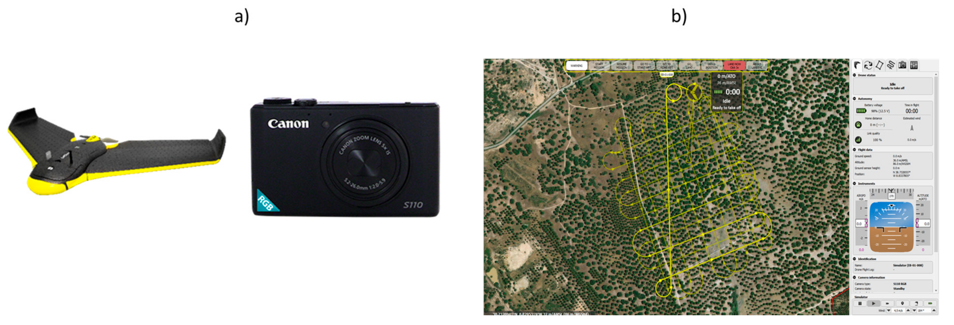
2.3. Remote Sensing Data Acquisition and Use

The airborne surveys were conducted by Terradrone Co. (Lisbon) on 12 March 2015 and 17 March 2017 using the same sensor, flight parameters and under similar (good) atmospheric conditions. In both surveys, an RGB camera was mounted on a fixed-wing UAV (SenseFly eBee) (Figure 2a). The RGB camera was a Canon Powershot S110 with a 4000 × 3000 pixel detector (Figure 2a), which captured images at ISO 200 and 1/2000 seconds with a 5.320 mm focal length and sensor dimension of 7.4 × 5.58 mm. It provided ~6 cm pixel⁻¹ resolution for an altitude of 170 m above ground level. The eMotion V. 3.2.4 flight planning and monitoring software was used to determine the main flight parameters (office-planning phase) (Figure 2b The flight plan covered the entire study area with a longitudinal and lateral overlaps of 80% and 75%, respectively. The flight line spacing was 48 m and each image covered an area of 240 × 180 m. The whole sets of 190 (year 2015) and 202 images (year 2017) were used to generate orthomosaics and digital surface models (DSMs) by the SfM image reconstruction process. The aerial data acquisition required greater control as it is important that the flights are always carried out under conditions of equal luminosity, a high degree of overlap and an covered area much larger than the selected area to avoid edge distortion [23,55].

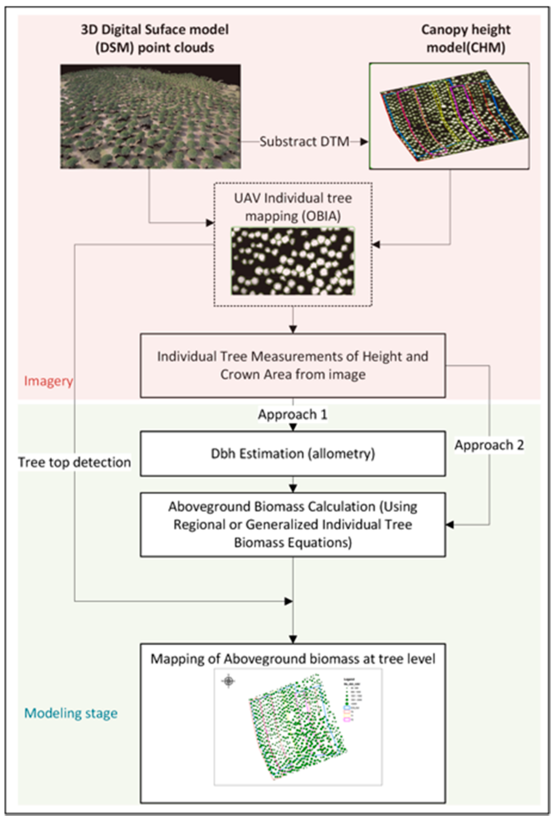
2.4. 3D Model Generation

The absolute orientation of the aerial photos was determined using aerotriangulation techniques performed by pix4D 3.1.22 (pix4D^®, Ecublens, Switzerland). Five (2015) and ten (2017) ground control points (GCPs) were measured in the field with topographic methods in order to georeference the SfM mosaic to a projected coordinate system. A LEICA GS15 GPS (Leica Geosystems, San Galo, Switzerland) (dual frequency, real time kinematic receiver with a planimetric precision of ±8 mm + 0.5 ppm and an altimetric precision of ±15 mm + 0.5 ppm) was used to capture the ground control photogrammetric target (marked with 60 × 60 cm matte white finish plastic boards detectable in RGB photographs). For reliable accuracy of GPS measurement, all GCPs were located in open areas with no canopy cover. At each point, GPS signals were logged in real time kinematic (RTK)—global navigation satellite system (GNSS) mode. The recordings were processed with real-time correction data retrieved from the fixed base station in Palmela (Lisbon) (latitude 38.5714631°, longitude −8.9034504°, and ellipsoidal elevation 245.989 m above the WGS84 reference ellipsoid). In 2015, GCPs were marked with surveying wooden stakes in order to relocate the centre of each point.

The photogrammetric point clouds were generated using the stereomatching algorithm implemented in pix4D 3.1.22. The matching parameters were set as follows: multiscale, image scale = 1/2 (half image size) and point density = ‘optimal’. We also set the minimum number of matched images to 3. Postflight Terra 3D project from 2015 was migrated to pix4D 3.1.22 in order to improve the accuracy of the digital elevation models (DEMs). Non-ground points were removed using the automatic object classification implemented in Pix4D. DEMs were generated from the ground points by using a natural neighbour interpolation technique implemented in Pix4D (additional details of the algorithms are proprietary and were not disclosed by Pix4D). Finally, one CHM was constructed for 2015 and another for 2017 by subtracting the DEMs from the DSMs point cloud using the FUSION LiDAR Toolkit [56].

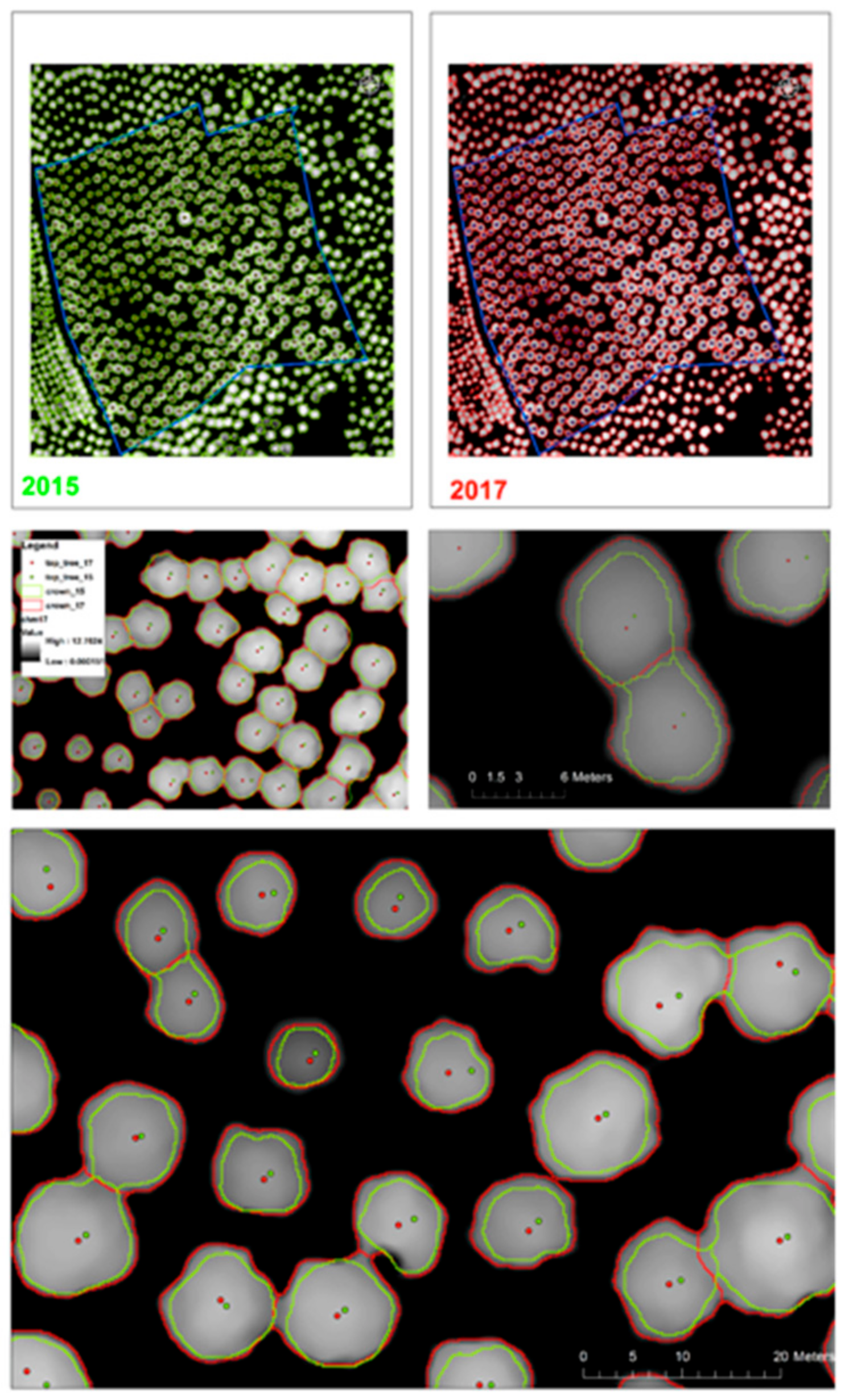
2.5. ITC Process and SfM-Derived Variables

Individual tree position (X and Y coordinates), height (h_SfM), and crown area (ca_SfM) were retrieved from the CHM (Figure 2). Resampling of the CHM to 20 cm resolution and subsequent smoothing with mean (5 × 5 window) and median filters (5 × 5 window) were conducted using the FUSION LiDAR Toolkit [56]. Crown delineation followed the procedure detailed in [42], but because of the forest stand and tree species characteristics, the initial maximum search domain in the iterative process (see Figure 3 in [42]) was changed from 5 to 25, and only one interaction was applied. Crown delineation results (Figure 3) and tree top positions were then exported in ESRI™ shapefiles as vector polygons and points, respectively, for subsequent analysis.

2.6. Individual Tree Biomass Estimation

Most biomass equations, including Equation (1), require measurement of tree diameter or circumference, which is not available from UAV imagery. We therefore tested two approaches for estimating SfM-derived individual-tree biomass (wa_SfM) (Figure 4). In the first approach, the multiplicative (power function) model in Equation (2), was fitted by using d as the dependent variable and h_SfM and ca_SfM as explanatory variables. Finally, the predicted diameter and h_SfM were included as explanatory variables in Equation (1) to predict wa_SfM for the subset of 50 trees. In the second approach, the multiplicative (power function) model in Equation (2) was also fitted to predict wa_SfM for the 50 trees, but wa (calculated using the field-measured d and h in Equation (1)) was used as a dependent variable, and h_SfM and ca_SfM were the explanatory variables.

$$Y={\beta }_0{X}_1{}^{{\lambda }_1}{X}_2{}^{{\lambda }_2}+\epsilon$$

(2)

where Y is the dependent variable, X₁ to X₂ are independent variables β₀ is the intercept, λ₁ and λ₂, are the exponential parameters to be estimated by non-linear regression analysis and ε is the additive term of the error. The models were fitted using the nls function implemented in the BASE package of R software (R Core Team, Vienna, Austria, 2016).

2.7. Accuraccy Analysis of the ITC and Individual Tree Variables

The ITC computations were validated in order to detect possible miscalculations in the image processing phase. We searched for false positives and/or false negatives using the method described by [57] and modified by [42] to link the SfM-detected trees to their corresponding field-measured trees. In order to assess the accuracy of SfM-detected tree heights, we plotted h vs h_SfM by using the correctly detected and linked trees and then visually inspected the graphs. We also compared d with d_SfM and wa with wa_SfM in the subsample of 50 trees for both 2015 and 2017. Finally, we computed the coefficient of determination (R²), the overall root mean square error (RMSE) and the relative root mean square error (rRMSE) to determine the accuracy of SfM for estimating tree heights, diameter and aboveground biomass in both 2015 and 2017.

2.8. Growth Analysis

A paired t-test was also conducted to compare SfM-predicted forest growth variables (tree height growth, Δh_SfM, and crown area growth, Δca_SfM) for the entire sample tree data set (N = 290) over one growth period (2015–2017) to determine whether the interval was sufficient to enable detection of statistically significant growth measurements in individual trees. The normality of the residuals of SfM-predicted forest growth variables was tested using the Shapiro-Wilk Test [58].

One-way ANOVA was used to analyze the effect of the fertirrigation treatments on the mean Δh_SfM and Δca_SfM and to assess the validity of the UAV-based DAP method to detect differences in forest growth related to the treatments. We included a random plot effect, to account for the lack of independence of trees measured within a plot, and a random block effect. The experimental data were analysed using SAS 9.4 (SAS Institute, Cary, NC, USA, 2012), with the proc mixed procedure and restricted maximum likelihood and the Kenward-Roger correction for degrees of freedom. We also used Tukey’s test for multiple pairwise comparisons to identify any significant differences between the treatments.

3. Results

3.1. Accuracy Analysis of the 3D Data Cloud

Table 2. Properties and planimetric and altimetric accuracy of the point clouds derived from the RGB imagery by using SfM.

Dataset	No. of GCPs	Density (Points m−2)	RMSEX (m)	RMSEY (m)	RMSEZ (m)
2015	5	65.3	0.0332	0.0568	0.0485
2017	10	64.9	0.0266	0.00693	0.0208
	5 (check points)		0.0446	0.00936	0.0439

GPCs: Ground Control Points (GCPs), RMSE_X, RMSE_Y and RMSE_Z are the root mean square error in the direction of the three spatial coordinates (X, Y and Z), reflecting the planimetric and altimetric accuracy.

shows the properties of the point clouds produced in 2015 and 2017. The total processing time required to produce a georeferenced point cloud from RGB images, using pix4D 3.1.22 installed on a dual Intel^®Core i7-3630QM workstation with 8 GB of RAM, was approximately 3 h. The point density of the SfM point cloud was 65.3 and 64.9 points m⁻² (Quick Terrain Reader, v 8.0.5.2) for 2015 and 2017, respectively. The observed planimetric and altimetric errors for the GCPs collected are shown in Table 2. In 2017, 5 independent GCPs were also used as check points to validate the accuracy of the geo-referenced point clouds (check points).

3.2. Field and SfM Biomass Estimation

The parameter estimates and goodness-of-fit statistics of the model used to predict wa (kg) as the sum of the biomass components (stem, bark, needles and branches), with c (cm) and h (m) as explanatory variables (Equation (1)) are shown in

Table 3. Estimated parameters and goodness-of-fit statistics for the model selected for estimating individual tree aboveground biomass.

Dependent Variable	Equation	Independent Variable (Parameter)	Parameter Estimate	Std. Error	p > |t|	Mef	RMSE	RMSE (%)
ww	Multiplicative component (Equation (1))	β0	1.16	0.261	<0.0001	0.94	117.4
		c (λ1)	2.27	0.0734	<0.0001
		h (λ2)	2.15	0.0738	<0.0001
wb	1st Additive component (Equation (1))	β1	23.8	8.585	0.0072	0.85	21.36
		c (λ3)	2.91	0.462	<0.0001
wl	2nd Additive component (Equation (1))	β2	39.4	6.50	<0.0001	0.88	38.44
		c (λ4)	3.17	0.209	<0.0001
wbr	3rd Additive component (Equation (1))	β3	215	13.2	<0.0001	0.72	123.4
		c (λ5)	1.52	0.0856	<0.0001
wa	ww + wb + wl + wbr (Equation (1))					0.96	163.7	33.53

w_w is the individual tree stem wood biomass (kg), w_b is the individual tree stem bark biomass (kg), w_l is the individual tree needle biomass (kg), w_br is the individual tree branch biomass (kg), w_a is the individual tree aboveground biomass (kg), d is the diameter at breast height (cm), c is the stem circumference at breast height (π*d/100) (m), h is the individual tree height (m), Mef is the model efficiency statistic and RMSE is the root mean square error.

.

The model represents an improvement in terms of Mef relative to previous models used to predict individual tree aboveground biomass in P. pinea plantations in Portugal [54] and it is also more representative, as the sample size is larger, including 35 additional data points. The RMSE was 163.7 kg, with a model efficiency (Mef) of 0.96 (Equation (1), Table 3). The improved model was applied to estimate wa for the subsample of 50 trees.

Table 4. Models selected for estimating SfM-derived individual tree diameter and SfM-derived individual tree aboveground biomass.

Dependent Variable	Equation	Independent Variable (Parameter)	Parameter Estimate	Standard Error	p > |t|	Mef	RMSE (cm)	RMSE (%)
d2015	Multiplicative (Equation (1))	β0 parameter	7.10059	1.17034	<0.0001	0.79	2.23	4.99
		hSfM (λ1)	0.35057	0.10825	0.0022
		caSfM (λ2)	0.23006	0.03661	<0.0001
d2017	Multiplicative (Equation (1))	β0 parameter	5.99931	1.04605	<0.0001	0.79	2.36	5.60
		hSfM (λ1)	0.41024	0.09869	<0.0001
		caSfM (λ2)	0.23775	0.03370	<0.0001
Dependent Variable	Equation	Independent Variable	Parameter Estimate	Standard Error	p > |t|	Mef	RMSE (Kg)	RMSE (%)
waSfM2015	Multiplicative (Equation (2))	β0 parameter	2.44131	0.93930	0.0124	0.85	87.46	11.44
		hSfM (λ1)	1.63850	0.23857	<0.0001
		caSfM (λ2)	0.47852	0.07782	<0.0001
waSfM20177	Multiplicative (Equation (2))	β0 parameter	1.11449	0.49991	0.0306	0.84	117.8	12.59
		hSfM (λ1)	1.97592	0.08079	<0.0001
		caSfM (λ2)	0.49129	0.24338	<0.0001

wa_SfM is the SfM aboveground biomass (kg), d is the diameter at breast height (cm), h_SfM is tree height from UAV imagery (m), ca_SfM is crown area from UAV imagery (m²), Mef is the model efficiency statistic and RMSE is the root mean squared error.

shows the parameter estimates and goodness-of-fit statistics for the models used to predict d (cm) and wa_SfM (kg) in 2015 and 2017 by approach 1 and the parameter estimates and goodness-of-fit statistics of the model used to predict wa_SfM (kg) in 2015 and 2017 by approach 2 (see the description of both approaches in Section 2.6. Individual tree biomass estimation).

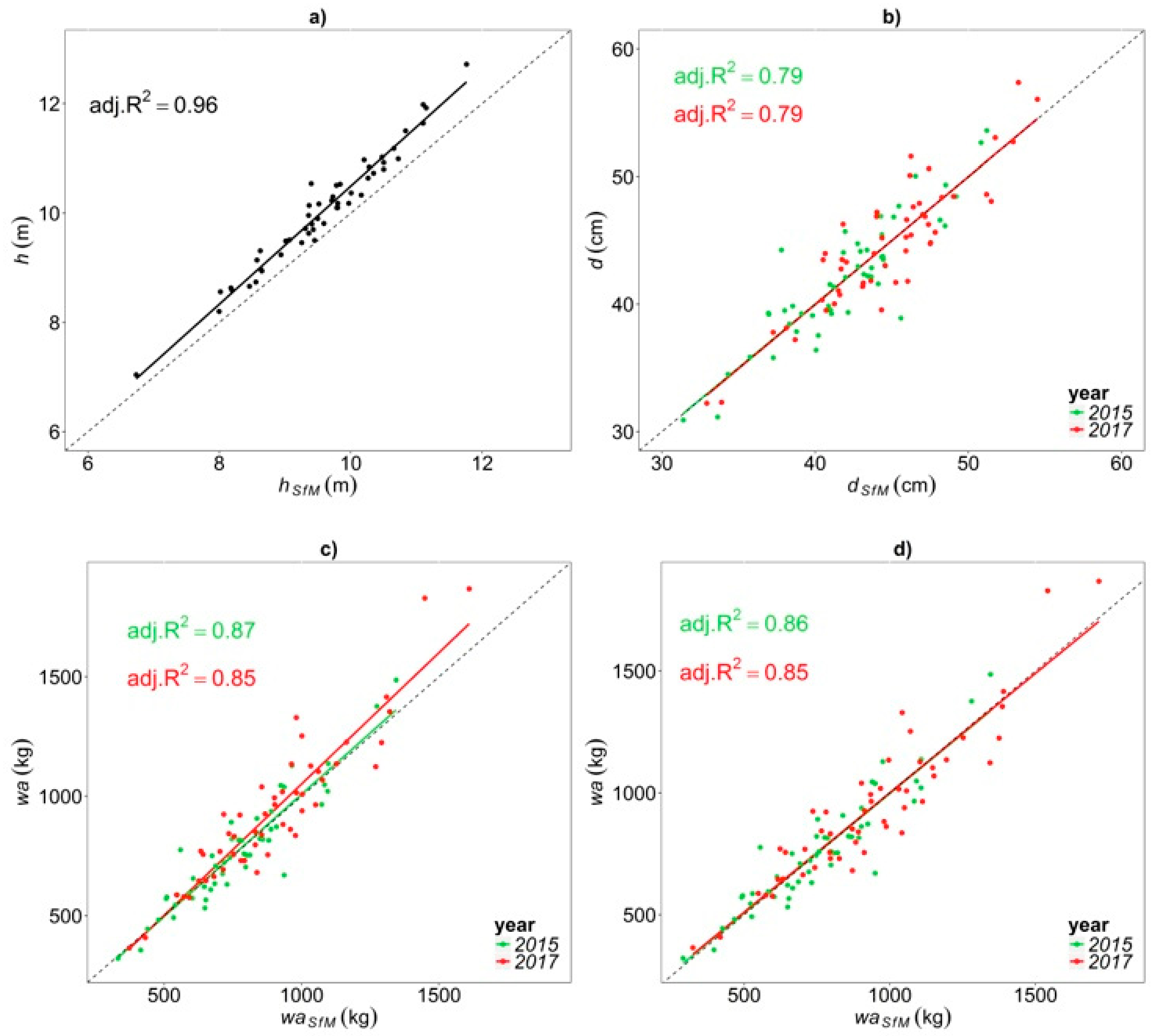
3.3. Accuracy Analysis of the ITC and Individual Tree Variables

We tested the accuracy of the ITC delineation by comparing and plotting h and h_SfM. The linear regressions between these two variables yielded an R² value of 0.96 and an RMSE value of 0.19 cm with an rRMSE of 1.89% for trees with field-measured height ranging between 7.00 and 12.72 m (Figure 5a). We also checked the overall detection rate, which was 100%, with no false positives or negatives. UAV-based DAP methods tended to underestimate tree height, relative to field measurements (vertex and telescopic pole), for both 2015 and 2017. Although d is not directly measured in CHMs derived from UAV, SfM-derived variables, especially ca_SfM, were strongly correlated with d (Figure 5b). The diameter predicted by Equation (2) was regressed against d, explaining 79% of the variability for both years (Figure 4b). There was no appreciable bias throughout the observed diameter range. The linear regression model that predicted wa_SfM by following approach 1 explained 87% (2015) and 85% (2017) of the variability (Figure 5c). However, this approach seemed to underestimate field above-ground biomass for 2017, especially for the largest trees (Figure 5c). Finally, the wa_SfM predicted by approach 2 explained 86% and 85% of the variability in 2015 and 2017, respectively, and did not show any appreciable bias (Figure 5d).

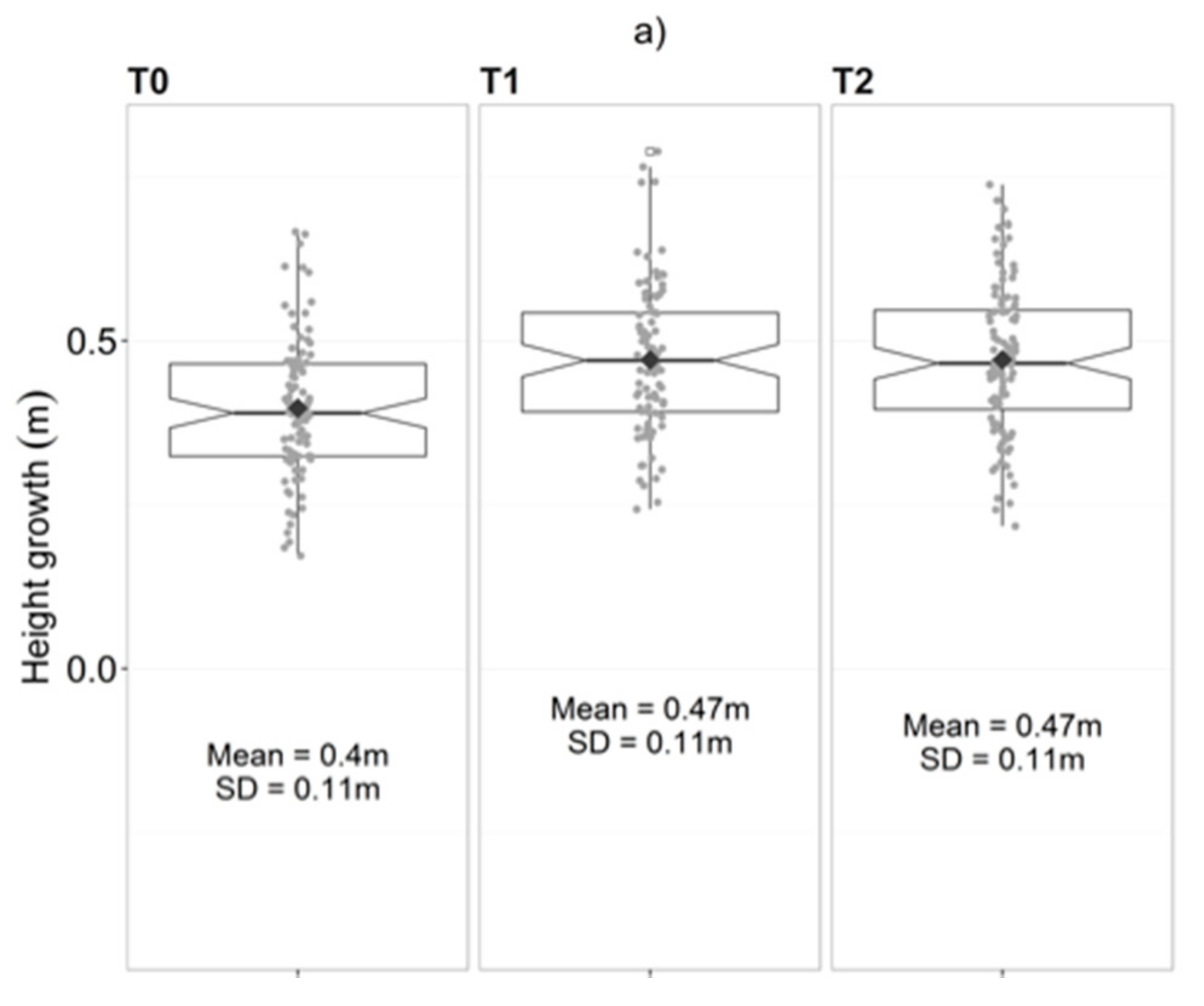
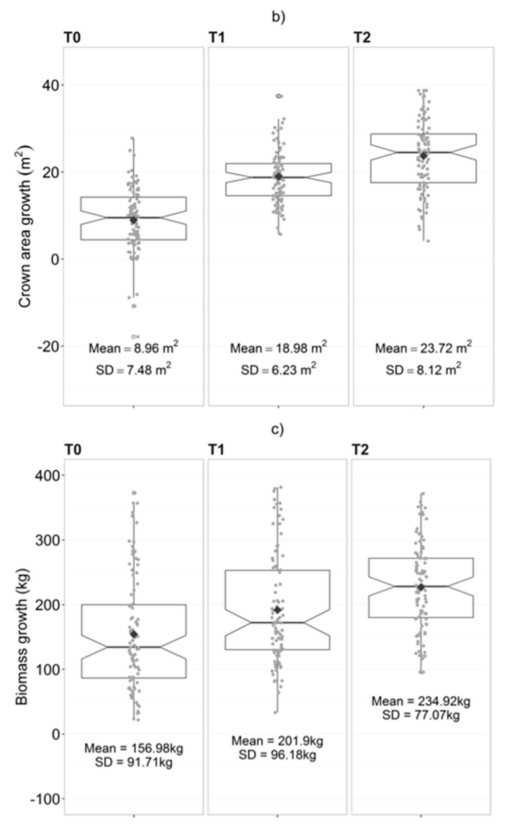
3.4. Growth Analysis

There was a statistically significant difference between SfM-predicted forest growth variables (Δh_SfM, Δca_SfM and Δwa_SfM) for the individual tree sample (N = 290) after two growing seasons (2015–2017). The mean annual Δh_SfM was 0.45 m, with a 95% CI between 0.43 and 0.47 m. The mean annual Δca_SfM was 17.29 m², with a 95% CI between 16.17 m² and 18.40 m² (

Table 5. Estimated image-based growth associated with each treatment for the entire dataset (N = 96 (T0); N = 94 (T1), N = 100 (T2)).

Plot	hSfM (n = 289)			caSfM			waSfM
	hSfM in 2015 (m)	hSfM in 2017 (m)	ΔhSfM (m)	caSfM in 2015 (m2)	caSfM in 2017 (m2)	ΔcaSfM (m2)	waSfM in 2015 (kg)	waSfM in 2017 (kg)	ΔwaSfM (kg)
T0 (mean)	9.56	9.95	0.40	83.15	92.11	8.96	830.4	987.4	157.0
T1 (mean)	9.14	9.63	0.47	79.08	98.05	18.98	754.7	957.4	202.7
T2 (mean)	9.44	9.92	0.47	89.59	113.31	23.72	844.9	1081.5	236.6
min	6.38	6.73	0.17	14.96	25.56	−17.84	155.7	263.2	21.9
max	11.86	12.36	0.79	169.76	190.28	38.75	1500.1	1922.2	448.9
mean	9.39	9.83	0.45	84.05	101.35	17.29	810.0	1008.8	198.7
SD	1.07	1.08	0.12	28.78	31.61	9.58	262.5	338.7	93.9
t-test p-value			<0.01			<0.01			<0.01

). Finally, the average aboveground biomass production for the 2-year period at the individual tree level was 189.7 kg, with a 95% CI between 187.57 kg and 209.26 kg (estimate is derived from the second approach, Equation (2), Table 4).

Height growth was detected for all 290 trees, but with a reduction in crown area in 5 trees (Table 5, Figure 6a,b). We observed small differences in the mean Δh_SfM between the treatments, with an average difference of 7 cm between the control and the combined fertirrigation treatments. For Δh_SfM, one extreme positive outlier, corresponding to a small tree for treatment T1 in plot 2 (probably due to an error in obtaining the single tree height in 2015) was removed from the analysis. The differences in mean Δwa_SfM and particularly in Δca_SfM were more evident (Figure 6b,c, respectively). The negative values in Δca_SfM were checked in the field and were explained by a variety of causes, including a dead tree, strong competition with neighbouring trees, and trees with large fallen branches. In terms of stand level biomass, the differences amounted to 3.86 Mg ha⁻¹ year⁻¹, 4.45 Mg ha⁻¹ year⁻¹ and 5.62 Mg ha⁻¹ year⁻¹ for T0, T1 and T2, respectively.

There was no evidence of any effect of the fertirrigation treatments on Δh_SfM and Δwa_SfM (p-values of 0.27 and 0.21, respectively, both based on an F-test on 2 and 2 degrees of freedom). Although tree growth was greatest in the fertilized and irrigated plots, the small sample size (only 6 plots and 2 degrees of freedom for the error) yielded a low power and a lack of ability to detect differences between treatments. However, we found a significant difference in Δca_SfM (p = 0.04). Tukey-Kramer’s test for multiple pairwise comparisons revealed that T1 and T2 were statistically significantly different from the control (T0), but not from each other.

4. Discussion

The spatial accuracy of the 3D cloud data is important to ensure a good description of tree crowns and was therefore a key issue in this study. Given the possible use of UAVs for monitoring vegetation dynamics, accurate direct georeferencing is an important processing step in forest areas [18,59,60]. Few studies have examined the effect of the sample size of GCPs on the accuracy of photogrammetric projections from UAVs [60,61]. We observed very small horizontal and vertical differences in accuracy with 5 or 10 GCPs (Table 1), as reported in other studies in flat terrain [61]. The mean RMSE_X, RMSE_Y, and RMSE_Z values for 10 CGPs were 0.026, 0.007 and 0.020 m, respectively. These values are slightly better than those obtained using a rotatory-wing UAV with 10 CGPs and a flight altitude of 120 m [61], but slightly worse, in terms of horizontal and vertical accuracy (0.007 m, 0.005 cm, and 0.014 cm, respectively), than those reported for a fixed-wing UAV in a boreal conifer forest, with 13 GCPs, a flight altitude of 120 m, and an average slope of 10° [19]. Our study findings confirm that horizontal and vertical accuracy increases with the number of GCPs. Furthermore, the RMSEz values increased with flight altitude, in agreement with the vertical RMSEz trend observed in a previous study [61].

The findings of the present study showed that individual tree variables (h_SfM, d_SfM and wa_SfM) could be estimated automatically from high resolution imagery, suggesting promising research lines for fast, reliable and cost-effective annual monitoring of P. pinea plantations that could help assess the efficiency of silvicultural treatments. The h_SfM estimation was similar to or better than that of previous studies uding SfM point clouds in palm plantations [62], olive orchards [4,24], boreal forests [32] and Eucalyptus forest [18]. The proposed methodology could be helpful in P. pinea forest management, as estimation of annual tree height growth from field data (Δh) in this species is extremely difficult. Indeed, we were not able to validate the Δh, because of the large measurement errors observed using hypsometers in 2015, reaching approximately 0.5 m [53]. In 2017, although we significantly improved the method of measuring h in the field in order to validate h_SfM, the CHM still slightly underestimated h. These observations are consistent with those of other studies working with DAP [63,64,65], DAP-UAV [20,66,67] and ALS [46,47,68,69] point cloud data. The following factors may partly explain the differences between h and h_SfM: (i) inaccuracies or bias in field-measured h caused by the difficulty in determining the top of the P. pinea trees due to their umbrella-shaped crown and lack of clear apical dominance; (ii) The developed-DEM from unsupervised ground-classified points filtering implemented in Pix4D 3.1.22 performed well in this flat area; however, the poor performance of the SfM photogrammetric technique for capturing the terrain surface below closed canopy cover, possibly leading to overestimation of the ground elevation [20,66,67] and underestimation of h_SfM; and (iii) smoothing of the image processing during the ITC process (necessary for noise reduction), possibly resulting in slight underestimation of h_SfM.

Field measurements are traditionally considered ground-truth values and are used as reference values for comparisons with remote-sensing estimates. However, some field measurements, such as h and ca, have unavoidable associated error and large variation [2,4,5,6] and thus may not be suitable for validation of the SfM-derived tree growth measurements, especially in dense stands or for trees which do not have well-defined top [70]. In our study, h_SfM was less variable than field-based measurements in both 2015 and 2017. Field h was measured to the nearest 0.1 m, while h_SfM was measured from tree apexes detected to the nearest 0.01 m. Field-measured h standard deviations were 1.05 m and 1.02 m in 2015 and 2017, respectively, while h_SfM standard deviations ranged from 0.92 m to 0.98 m, in 2015 and 2017, respectively. Future research should consider the combined use of UAV and LiDAR to improve the DEM/CHM generation, as well as the combination of GPS and total station measurements to obtain ground-truth values of the forest variables and ground point under the canopy for improved quantification of the errors. A recent study has already demonstrated improvements of up to 40 cm in tree height measurement using LiDAR/UAV instead of UAV imagery in a dry sclerophyll eucalypt forest within areas of relatively low canopy closure [18]. Another solution might be to consider 1 or 2 points per square meter under canopy using a lightweight, cost effective rangefinder with the ability to log and co-register image-based point clouds.

The wa_SfM was accurately estimated from UAV-based DAP using both approaches (approaches 1 and 2, described in Section 2.6. Individual tree biomass estimation). Individual tree variables derived from the automated processing of UAV imagery and ITC delineation, such as h_SfM and ca_SfM, were found to be significant explanatory variables for predicting d and wa. Studies conducted in Picea abeis (L.) H. Karst. and Pinus sylvestris L. stands in Sweden and in Pinus taeda L. stands in the SE United States found that ALS-derived h and crown diameter (cd) explained up to 87% and 91% of the variance associated with the estimation of d, with an RMSE of 3.8 and 4.9 cm, respectively [41,57]. Zhao et al. [71] reported an adj. R² value of 0.87 and an RMSE value of 5.2 cm for ALS-derived tree dimension variables including h, cd and crown base height in P. taeda stands. In this study, the diameter equation based on SfM-derived variables performed well, although the values of Mef are slightly lower than some of those reported for other species [41,57]. The performance of the wa_SfM estimates for predicting tree biomass directly from SfM-derived variables (approach 2, adj. R² = 0.86–0.85, RMSE = 87.46–117.8 kg) was similar to that obtained by [41] (R² = 0.88, RMSE = 169 kg) and slightly better than those for P. taeda (R² = 0.80, RMSE = 237 kg) [71]. For wa_SfM, the potential sources of error and variation may be similar to those already discussed for h_SfM and ca_SfM. Specifically, the tendency of SfM to underestimate h may be the main reason for underestimation of wa_SfM with approach 1 in 2017. The allometric relationship between wa_SfM and SfM crown-derived variables could be refined, either by harvesting more trees or through improvements in UAV imagery processing.

The results of the growth analysis demonstrated that the resolution of the photogrammetric point clouds obtained by stereomatching aerial photographs would be sufficient for estimating Δh_SfM, Δca_SfM and Δwa_SfM in P. pinea plantations, because low-altitude flights can be carried out with UAVs. The relatively short period between data collection (2015–2017), and the relatively slow tree height growth rate of this species at this age, may also have led to some inaccuracy as measurement and precision errors may be within the physical limits of tree growth. The mean annual Δh_SfM computed using 96 trees within T0 treatment was 0.20 m year⁻¹, lower than the published site index 21 growth rate of 0.28 m year⁻¹ derived from the forest growth model for this species [72]. The mean annual Δwa_SfM from high resolution images showed that, during the experimental period, fertirrigation increased the biomass growth rate of P. pinea plantations, relative to the unfertilized treatment (T0), but the small sample size led to a low level of statistical power for detecting differences after 2 years of treatment (Figure 5). It was possible to estimate the annual biomass increment at tree level because the h_SfM was considered as a ground-truth value in 2015, following the methodology of recent published studies [50]. Goodbody et al. [50] estimated the mean gross tree volume increments considering h and ca directly from CHMs derived from light UAV-based DAP and LiDAR, respectively. Use of the PINEA.pt growth model [73] implemented in the forest growth simulator (StandSIM module) [74,75] with an input tree file for the existing stand structure (Stem density = 54 tree ha⁻¹, Stand age = 24 and Site index = 21) in the study area showed that the mean annual aboveground biomass production (3.9 Mg ha⁻¹ year⁻¹) was similar to the estimated biomass growth in the control (3.86 Mg ha⁻¹ year⁻¹). Estimates were within the limits of forest growth models [74,75] and local independent field measured sample plot. UAV-DAP point clouds were therefore effective for updating individual tree growth and biomass between 2015 and 2017. The results also show a hierarchical growth habit in this species due to a lower level of apical dominance of the leader shoot than in most other conifers [76].

It was also possible to detect differences in biomass yield under different treatments. Our findings are consistent with those of previous studies, which investigated the effects of fertilization on the biomass allocation of hardwood species [77,78,79]. Albaugh et al. [79] used data from nine sites in which nutrient and water optimization studies were carried out with a 2 × 2 factorial design to determine maximum biomass production in response to a simple set of treatments. These authors found that above-ground, stem and total biomass production ranged from 3 to 30, 2 to 28, and 5 to 32 Mg ha⁻¹ year⁻¹, respectively. In the present study, above-ground production (Δwa_SfM = 5.62 Mg ha⁻¹ year⁻¹) was within the range reported for fertirrigation treatment in other species, although at different ages and considering only the effect of two years of treatment. For example, the values of wa_SfM were lower than for 4-year-old P. taeda receiving fertilization and water treatments [80] (6.9 Mg ha⁻¹ year⁻¹) after three growing seasons in the southeastern United States and those reported by [81] (10 Mg ha⁻¹ year⁻¹) and up to 18 Mg ha⁻¹ year⁻¹ [82] in a 2-year-old stand and 8-year-old stand of P. taeda after the 6th and 4th year of treatment, respectively. The fertirrigation treatment (T2) increased above-ground biomass increment, with growth responses reaching up to 51% of that the control. This value is similar to that reported for a P. pinaster plantation in south-western France (5-year-old stand) after five years of treatment [83]. These differences may reflect differences in initial site fertility and climate, as well as the responsiveness of the species to nutrient treatments.

Finally, inferences from multi-temporal images could also be improved by carrying out the flights on almost the same date, under similarly good atmospheric conditions, and using similar image-acquisition parameters. In this study, this methodology was applied on flat terrain, in open canopies with no understory. In natural and managed closed-canopy forests and steeper terrain, poorer performance could be expected, as aerial photography cannot penetrate vegetation, and additional ALS data may therefore be needed. In order to ameliorate such errors in future studies, an approach using broad scale ALS acquisition at 10 year intervals, with regular 4–6 year UAS-DAP point cloud updates for mature stands, could be applied [50,84].

5. Conclusions

This study shows that multi-temporal UAV datasets and SfM techniques are promising tools for monitoring individual tree variables, forest and biomass growth and, ultimately, supporting decisions regarding the management of P. pinea forests. Future research with multi-temporal UAV datasets could benefit from the knowledge provided in this study, which reports the monitoring of spatial and temporal processes, analysis of individual tree-level competition, growth and effects of the treatments and forest management practices in P. pinea stands. The proposed methodology could help in the management of P. pinea forest and woodland-pasture ecosystems, as estimation of tree height growth from field data in this species is extremely difficult due to the lack of strong apical dominance and an umbrella-shaped crown. The study findings represent progress in the use of high resolution UAV imagery for estimate forest tree variables and forest growth, improving the temporal resolution of the forest inventories, reducing their cost and in some cases improving the accuracy of the forest variable estimates. In summary, this study has shown the potential of multi-temporal UAV data to characterize forest growth and to estimate biomass in Mediterranean P. pinea plantations.

References

1. Burkhart, H.E.; Tomé, M. Modeling Forest Trees and Stands; Springer Science & Business Media: Berlin, Germany, 2012. [Google Scholar]
2. Thenkabail, P.S.; Durrieu, S.; Véga, C.; Bouvier, M.; Gosselin, F.; Renaud, J.-P.; Saint-André, L. Optical remote sensing of tree and stand heights. In Land Resources Monitoring, Modeling, and Mapping with Remote Sensing; CRC Press: Boca Raton, FL, USA, 2015; pp. 449–485. [Google Scholar]
3. Sibona, E.; Vitali, A.; Meloni, F.; Caffo, L.; Dotta, A.; Lingua, E.; Motta, R.; Garbarino, M. Direct measurement of tree height provides different results on the assessment of LiDAR accuracy. Forests 2016, 8, 7. [Google Scholar] [CrossRef]
4. Díaz-Varela, R.A.; de la Rosa, R.; León, L.; Zarco-Tejada, P.J. High-resolution airborne UAV imagery to assess olive tree crown parameters using 3D photo reconstruction: Application in breeding trials. Remote Sens. 2015, 7, 4213–4232. [Google Scholar] [CrossRef]
5. Williams, M.S.; Bechtold, W.A.; LaBau, V.J. Five instruments for measuring tree height: An evaluation. South. J. Appl. For. 1994, 18, 76–82. [Google Scholar]
6. Panagiotidis, D.; Abdollahnejad, A.; Surový, P.; Chiteculo, V. Determining tree height and crown diameter from high-resolution UAV imagery. Int. J. Remote Sens. 2016, 38, 2392–2410. [Google Scholar] [CrossRef]
7. White, J.C.; Coops, N.C.; Wulder, M.A.; Vastaranta, M.; Hilker, T.; Tompalski, P. Remote sensing technologies for enhancing forest inventories: A review. Can. J. Remote Sens. 2016, 42, 619–641. [Google Scholar] [CrossRef]
8. Baltsavias, E.P. A comparison between photogrammetry and laser scanning. ISPRS J. Photogramm. Remote Sens. 1999, 54, 83–94. [Google Scholar] [CrossRef]
9. Næsset, E. Determination of mean tree height of forest stands by digital photogrammetry. Scand. J. For. Res. 2002, 17, 446–459. [Google Scholar] [CrossRef]
10. Næsset, E. Predicting forest stand characteristics with airborne scanning laser using a practical two-stage procedure and field data. Remote Sens. Environ. 2002, 80, 88–99. [Google Scholar] [CrossRef]
11. St-Onge, B.; Vega, C.; Fournier, R.A.; Hu, Y. Mapping canopy height using a combination of digital stereo-photogrammetry and lidar. Int. J. Remote Sens. 2008, 29, 3343–3364. [Google Scholar] [CrossRef]
12. Bohlin, J.; Wallerman, J.; Fransson, J.E. Forest variable estimation using photogrammetric matching of digital aerial images in combination with a high-resolution DEM. Scand. J. For. Res. 2012, 27, 692–699. [Google Scholar] [CrossRef]
13. White, J.C.; Wulder, M.A.; Vastaranta, M.; Coops, N.C.; Pitt, D.; Woods, M. The utility of image-based point clouds for forest inventory: A comparison with airborne laser scanning. Forests 2013, 4, 518–536. [Google Scholar] [CrossRef]
14. Fritz, A.; Kattenborn, T.; Koch, B. UAV-based photogrammetric point clouds—Tree stem mapping in open stands in comparison to terrestrial laser scanner point clouds. Int. Arch. Photogramm. Remote Sens. Spat. Inf. Sci. 2013, 40, 141–146. [Google Scholar] [CrossRef]
15. Gobakken, T.; Bollandsås, O.M.; Næsset, E. Comparing biophysical forest characteristics estimated from photogrammetric matching of aerial images and airborne laser scanning data. Scand. J. For. Res. 2014, 30, 73–86. [Google Scholar] [CrossRef]
16. Wallace, L.; Lucieer, A.; Watson, C.; Turner, D. Development of a UAV-LiDAR system with application to forest inventory. Remote Sens. 2012, 4, 1519–1543. [Google Scholar] [CrossRef]
17. Lisein, J.; Pierrot-Deseilligny, M.; Bonnet, S.; Lejeune, P. A photogrammetric workflow for the creation of a forest canopy height model from small unmanned aerial system imagery. Forests 2013, 4, 922–944. [Google Scholar] [CrossRef]
18. Wallace, L.; Lucieer, A.; Malenovský, Z.; Turner, D.; Vopěnka, P. Assessment of forest structure using two UAV techniques: A comparison of airborne laser scanning and structure from motion (SfM) point clouds. Forests 2016, 7, 62. [Google Scholar] [CrossRef]
19. Puliti, S.; Ørka, H.O.; Gobakken, T.; Næsset, E. Inventory of small forest areas using an unmanned aerial system. Remote Sens. 2015, 7, 9632–9654. [Google Scholar] [CrossRef] [Green Version]
20. Dandois, J.P.; Ellis, E.C. High spatial resolution three-dimensional mapping of vegetation spectral dynamics using computer vision. Remote Sens. Environ. 2013, 136, 259–276. [Google Scholar] [CrossRef]
21. Whitehead, K.; Hugenholtz, C.H. Remote sensing of the environment with small unmanned aircraft systems (UASs), Part 1: A review of progress and challenges. J. Unmanned Veh. Syst. 2014, 2, 69–85. [Google Scholar] [CrossRef]
22. Tang, L.; Shao, G. Drone remote sensing for forestry research and practices. J. For. Res. 2015, 26, 791–797. [Google Scholar] [CrossRef]
23. Baltsavias, E.; Gruen, A.; Eisenbeiss, H.; Zhang, L.; Waser, L.T. High-quality image matching and automated generation of 3D tree models. Int. J. Remote Sens. 2008, 29, 1243–1259. [Google Scholar] [CrossRef]
24. Zarco-Tejada, P.J.; Diaz-Varela, R.; Angileri, V.; Loudjani, P. Tree height quantification using very high resolution imagery acquired from an Unmanned Aerial Vehicle (UAV) and automatic 3D photo-reconstruction methods. Eur. J. Agron. 2014, 55, 89–99. [Google Scholar] [CrossRef]
25. Hall, S.A.; Burke, I.C.; Box, D.O.; Kaufmann, M.R.; Stoker, J.M. Estimating stand structure using discrete-return lidar: An example from low density, fire prone ponderosa pine forests. For. Ecol. Manag. 2005, 208, 189–209. [Google Scholar] [CrossRef]
26. Véga, C.; St-Onge, B. Height growth reconstruction of a boreal forest canopy over a period of 58 years using a combination of photogrammetric and lidar models. Remote Sens. Environ. 2008, 112, 1784–1794. [Google Scholar] [CrossRef] [Green Version]
27. Järnstedt, J.; Pekkarinen, A.; Tuominen, S.; Ginzler, C.; Holopainen, M.; Viitala, R. Forest variable estimation using a high-resolution digital surface model. ISPRS J. Photogramm. Remote Sens. 2012, 74, 78–84. [Google Scholar] [CrossRef]
28. Vastaranta, M.; Wulder, M.A.; White, J.C.; Pekkarinen, A.; Tuominen, S.; Ginzler, C.; Kankare, V.; Holopainen, M.; Hyyppä, J.; Hyyppä, H. Airborne laser scanning and digital stereo imagery measures of forest structure: Comparative results and implications to forest mapping and inventory update. Can. J. Remote Sens. 2013, 39, 382–395. [Google Scholar] [CrossRef]
29. Pitt, D.G.; Woods, M.; Penner, M. A comparison of point clouds derived from stereo imagery and airborne laser scanning for the area-based estimation of forest inventory attributes in Boreal Ontario. Can. J. Remote Sens. 2014, 40, 214–232. [Google Scholar] [CrossRef]
30. González-Ferreiro, E.; Diéguez-Aranda, U.; Miranda, D. Estimation of stand variables in pinus radiata D. Don plantations using different LiDAR pulse densities. Forestry 2012, 85, 281–292. [Google Scholar] [CrossRef]
31. González-Ferreiro, E.; Diéguez-Aranda, U.; Crecente-Campo, F.; Barreiro-Fernández, L.; Miranda, D.; Castedo-Dorado, F. Modelling canopy fuel variables for pinus radiata D. Don in NW Spain with low-density LiDAR data. Int. J. Wildland Fire 2014, 23, 350–362. [Google Scholar] [CrossRef]
32. Ota, T.; Ogawa, M.; Shimizu, K.; Kajisa, T.; Mizoue, N.; Yoshida, S.; Takao, G.; Hirata, Y.; Furuya, N.; Sano, T. Aboveground biomass estimation using structure from motion approach with aerial photographs in a seasonal tropical forest. Forests 2015, 6, 3882–3898. [Google Scholar] [CrossRef]
33. Montaghi, A.; Corona, P.; Dalponte, M.; Gianelle, D.; Chirici, G.; Olsson, H. Airborne laser scanning of forest resources: An overview of research in Italy as a commentary case study. Int. J. Appl. Earth Obs. Geoinf. 2013, 23, 288–300. [Google Scholar] [CrossRef] [Green Version]
34. Corona, P.; Cartisano, R.; Salvati, R.; Chirici, G.; Floris, A.; Di Martino, P.; Marchetti, M.; Scrinzi, G.; Clementel, F.; Torresan, C. Airborne laser scanning to support forest resource management under alpine, temperate and mediterranean environments in Italy. Eur. J. Remote Sens. 2012, 45, 27–37. [Google Scholar] [CrossRef]
35. García, M.; Riaño, D.; Chuvieco, E.; Danson, F.M. Estimating biomass carbon stocks for a mediterranean forest in central spain using LiDAR height and intensity data. Remote Sens. Environ. 2010, 114, 816–830. [Google Scholar] [CrossRef]
36. González-Olabarria, J.-R.; Rodríguez, F.; Fernández-Landa, A.; Mola-Yudego, B. Mapping fire risk in the model forest of Urbión (Spain) based on airborne LiDAR measurements. For. Ecol. Manag. 2012, 282, 149–156. [Google Scholar] [CrossRef]
37. Guerra-Hernández, J.; Görgens, E.B.; García-Gutiérrez, J.; Carlos, L.; Rodriguez, E.; Tomé, M.; González-Ferreiro, E. Comparison of ALS based models for estimating aboveground biomass in three types of mediterranean forest. Eur. J. Remote Sens. 2016, 49, 185–204. [Google Scholar] [CrossRef]
38. Kachamba, D.J.; Ørka, H.O.; Gobakken, T.; Eid, T.; Mwase, W. Biomass estimation using 3D data from unmanned aerial vehicle imagery in a tropical woodland. Remote Sens. 2016, 8, 968. [Google Scholar] [CrossRef]
39. St-Onge, B.; Audet, F.-A.; Bégin, J. Characterizing the height structure and composition of a boreal forest using an individual tree crown approach applied to photogrammetric point clouds. Forests 2015, 6, 3899–3922. [Google Scholar] [CrossRef]
40. Hyyppä, J.; Inkinen, M. Detecting and estimating attributes for single trees using laser scanner. Photogramm. J. Finl. 1999, 16, 27–42. [Google Scholar]
41. Popescu, S.C. Estimating biomass of individual pine trees using airborne lidar. Biomass Bioenergy 2007, 31, 646–655. [Google Scholar] [CrossRef]
42. González-Ferreiro, E.; Diéguez-Aranda, U.; Barreiro-Fernández, L.; Buján, S.; Barbosa, M.; Suárez, J.C.; Bye, I.J.; Miranda, D. A mixed pixel-and region-based approach for using airborne laser scanning data for individual tree crown delineation in pinus radiata D. Don plantations. Int. J. Remote Sens. 2013, 34, 7671–7690. [Google Scholar] [CrossRef]
43. Maltamo, M.; Næsset, E.; Vauhkonen, J. Forestry Applications of Airborne Laser Scanning; Springer: Berlin, Germany, 2014. [Google Scholar]
44. Hyyppä, J.; Hyyppä, H.; Leckie, D.; Gougeon, F.; Yu, X.; Maltamo, M. Review of methods of small-footprint airborne laser scanning for extracting forest inventory data in boreal forests. Int. J. Remote Sens. 2008, 29, 1339–1366. [Google Scholar] [CrossRef]
45. Næsset, E.; Gobakken, T. Estimating forest growth using canopy metrics derived from airborne laser scanner data. Remote Sens. Environ. 2005, 96, 453–465. [Google Scholar] [CrossRef]
46. Yu, X.; Hyyppä, J.; Kukko, A.; Maltamo, M.; Kaartinen, H. Change detection techniques for canopy height growth measurements using airborne laser scanner data. Photogramm. Eng. Remote Sens. 2006, 72, 1339–1348. [Google Scholar] [CrossRef]
47. Hopkinson, C.; Chasmer, L.; Hall, R.J. The uncertainty in conifer plantation growth prediction from multi-temporal lidar datasets. Remote Sens. Environ. 2008, 112, 1168–1180. [Google Scholar] [CrossRef]
48. Frew, M.S.; Evans, D.L.; Londo, H.A.; Cooke, W.H.; Irby, D. Measuring Douglas-fir crown growth with multitemporal LiDAR. For. Sci. 2015, 62, 200–212. [Google Scholar] [CrossRef]
49. Wang, Z.; Ginzler, C.; Waser, L.T. A novel method to assess short-term forest cover changes based on digital surface models from image-based point clouds. Forestry 2015, 88, 429–440. [Google Scholar] [CrossRef]
50. Goodbody, T.R.; Coops, N.C.; Marshall, P.L.; Tompalski, P.; Crawford, P. Unmanned aerial systems for precision forest inventory purposes: A review and case study. For. Chron. 2017, 93, 71–81. [Google Scholar] [CrossRef]
51. Dempewolf, J.; Nagol, J.; Hein, S.; Thiel, C.; Zimmermann, R. Measurement of within-season tree height growth in a mixed forest stand using UAV imagery. Forests 2017, 8, 231. [Google Scholar] [CrossRef]
52. Jiménez-Brenes, F.M.; López-Granados, F.; Castro, A.I.; Torres-Sánchez, J.; Serrano, N.; Peña, J.M. Quantifying pruning impacts on olive tree architecture and annual canopy growth by using UAV-Based 3D modelling. Plant Methods 2017, 13, 55. [Google Scholar] [CrossRef] [PubMed]
53. Guerra-Hérnandez, J.; González-Ferreiro, E.; Sarmento, A.; Silva, J.; Nunes, A.; Correia, A.C.; Fontes, L.; Tomé, M.; Díaz-Varela, R. Short Communication. Using High Resolution UAV Imagery to Estimate Tree Variables in Pinus Pinea Plantation in Portugal. For. Syst. 2016, 25, 09. [Google Scholar] [CrossRef]
54. Correia, A.C.; Tomé, M.; Carlos, P.; Sónia, F.; Dias, A.; Freire, J.; Carvalho, P.O.; Pereira, J.S. Biomass allometry and carbon factors for a mediterranean pine (Pinus pinea L.) in Portugal. For. Syst. 2010, 19, 418–433. [Google Scholar] [CrossRef]
55. Dandois, J.P.; Olano, M.; Ellis, E.C. Optimal altitude, overlap, and weather conditions for computer vision UAV estimates of forest structure. Remote Sens. 2015, 7, 13895–13920. [Google Scholar] [CrossRef]
56. McGaughey, R. FUSION/LDV: Software for LiDAR Data Analysis and Visualization, Version 3.41; US Department of Agriculture, Forest Service, Pacific Northwest Research Station: Seattle, WA, USA, 2014.
57. Persson, A.; Holmgren, J.; Söderman, U. Detecting and measuring individual trees using an airborne laser scanner. Photogramm. Eng. Remote Sens. 2002, 68, 925–932. [Google Scholar]
58. Shapiro, S.S.; Wilk, M.B.; Chen, H.J. A comparative study of various tests for normality. J. Am. Stat. Assoc. 1968, 63, 1343–1372. [Google Scholar] [CrossRef]
59. Turner, D.; Lucieer, A.; Wallace, L. Direct georeferencing of ultrahigh-resolution UAV imagery. IEEE Trans. Geosci. Remote Sens. 2014, 52, 2738–2745. [Google Scholar] [CrossRef]
60. Tomaštík, J.; Mokroš, M.; Saloň, Š.; Chudý, F.; Tunák, D. Accuracy of photogrammetric UAV-based point clouds under conditions of partially-open forest canopy. Forests 2017, 8, 151. [Google Scholar] [CrossRef]
61. Agüera-Vega, F.; Carvajal-Ramírez, F.; Martínez-Carricondo, P. Accuracy of digital surface models and orthophotos derived from unmanned aerial vehicle photogrammetry. J. Surv. Eng. 2016, 143, 04016025. [Google Scholar] [CrossRef]
62. Kattenborn, T.; Sperlich, M.; Bataua, K.; Koch, B. Automatic single tree detection in plantations using UAV-based photogrammetric point clouds. Int. Arch. Photogramm. Remote Sens. Spat. Inf. Sci. 2014, 40, 139. [Google Scholar] [CrossRef]
63. Korpela, I. Individual Tree Measurements by Means of Digital Aerial Photogrammetry; Finnish Society of Forest Science: Helsinki, Finland, 2004; Volume 3. [Google Scholar]
64. St-Onge, B.; Jumelet, J.; Cobello, M.; Véga, C. Measuring individual tree height using a combination of stereophotogrammetry and lidar. Can. J. For. Res. 2004, 34, 2122–2130. [Google Scholar] [CrossRef]
65. Tanhuanpää, T.; Saarinen, N.; Kankare, V.; Nurminen, K.; Vastaranta, M.; Honkavaara, E.; Karjalainen, M.; Yu, X.; Holopainen, M.; Hyyppä, J. Evaluating the performance of high-altitude aerial image-based digital surface models in detecting individual tree crowns in mature boreal forests. Forests 2016, 7, 143. [Google Scholar] [CrossRef]
66. Zahawi, R.A.; Dandois, J.P.; Holl, K.D.; Nadwodny, D.; Reid, J.L.; Ellis, E.C. Using lightweight unmanned aerial vehicles to monitor tropical forest recovery. Biol. Conserv. 2015, 186, 287–295. [Google Scholar] [CrossRef]
67. Jensen, J.L.; Mathews, A.J. Assessment of image-based point cloud products to generate a bare earth surface and estimate canopy heights in a woodland ecosystem. Remote Sens. 2016, 8, 50. [Google Scholar] [CrossRef]
68. Yu, X.; Hyyppä, J.; Kaartinen, H.; Maltamo, M. Automatic detection of harvested trees and determination of forest growth using airborne laser scanning. Remote Sens. Environ. 2004, 90, 451–462. [Google Scholar] [CrossRef]
69. Gatziolis, D.; Fried, J.S.; Monleon, V.S. Challenges to estimating tree height via LiDAR in closed-canopy forests: A parable from Western Oregon. For. Sci. 2010, 56, 139–155. [Google Scholar]
70. Luoma, V.; Saarinen, N.; Wulder, M.A.; White, J.C.; Vastaranta, M.; Holopainen, M.; Hyyppä, J. Assessing precision in conventional field measurements of individual tree attributes. Forests 2017, 8, 38. [Google Scholar] [CrossRef]
71. Zhao, K.; Popescu, S.; Nelson, R. Lidar remote sensing of forest biomass: A scale-invariant estimation approach using airborne lasers. Remote Sens. Environ. 2009, 113, 182–196. [Google Scholar] [CrossRef]
72. Calama, R.; Canadas, N.; Montero, G. Inter-regional variability in site index models for even-aged stands of stone pine (Pinus pinea L.) in Spain. Ann. For. Sci. 2003, 60, 259–269. [Google Scholar] [CrossRef]
73. Freire, J.P.A. Modelação Do Crescimento e Da Produção de Pinha No Pinheiro Manso; University of Lisbon: Lisbon, Portugal, 2009. [Google Scholar]
74. Faias, S.P.; Palma, J.H.N.; Barreiro, S.M.; Paulo, J.A.; Tomé, M. Resource communication. SIMfLOR–platform for portuguese forest simulators. For. Syst. 2012, 21, 543–548. [Google Scholar] [CrossRef]
75. Barreiro, S.; Rua, J.; Tomé, M. StandsSIM-MD: A management driven forest simulator. For. Syst. 2016, 25, 07. [Google Scholar] [CrossRef]
76. Mutke, S.; Calama, R.; González-Martínez, S.C.; Montero, G.; Gordo, F.J.; Bono, D.; Gil, L. Mediterranean stone pine: Botany and horticulture. Hortic. Rev. 2012, 39, 153–201. [Google Scholar]
77. Coyle, D.R.; Coleman, M.D.; Aubrey, D.P. Above-and below-ground biomass accumulation, production, and distribution of sweetgum and loblolly pine grown with irrigation and fertilization. Can. J. For. Res. 2008, 38, 1335–1348. [Google Scholar] [CrossRef]
78. Coyle, D.R.; Aubrey, D.P.; Coleman, M.D. Growth responses of narrow or broad site adapted tree species to a range of resource availability treatments after a full harvest rotation. For. Ecol. Manag. 2016, 362, 107–119. [Google Scholar] [CrossRef]
79. Albaugh, T.J.; Albaugh, J.M.; Fox, T.R.; Allen, H.L.; Rubilar, R.A.; Trichet, P.; Loustau, D.; Linder, S. Tamm review: Light use efficiency and carbon storage in nutrient and water experiments on major forest plantation species. For. Ecol. Manag. 2016, 376, 333–342. [Google Scholar] [CrossRef]
80. Coyle, D.R.; Coleman, M.D. Forest production responses to irrigation and fertilization are not explained by shifts in allocation. For. Ecol. Manag. 2005, 208, 137–152. [Google Scholar] [CrossRef]
81. Samuelson, L.J.; Johnsen, K.; Stokes, T. Production, Allocation, and Stemwood Growth Efficiency of Pinus taeda L. stands in response to 6 years of intensive management. For. Ecol. Manag. 2004, 192, 59–70. [Google Scholar] [CrossRef]
82. Adegbidi, H.G.; Jokela, E.J.; Comerford, N.B.; Barros, N.F.D. Biomass development for intensively managed loblolly pine plantations growing on Spodosols in the southeastern USA. For. Ecol. Manag. 2002, 167, 91–102. [Google Scholar] [CrossRef]
83. Trichet, P.; Loustau, D.; Lambrot, C.; Linder, S. Manipulating nutrient and water availability in a maritime pine plantation: Effects on growth, production, and biomass allocation at canopy closure. Ann. For. Sci. 2008, 65, 814. [Google Scholar] [CrossRef]
84. White, J.C.; Stepper, C.; Tompalski, P.; Coops, N.C.; Wulder, M.A. Comparing ALS and image-based point cloud metrics and modelled forest inventory attributes in a complex coastal forest environment. Forests 2015, 6, 3704–3732. [Google Scholar] [CrossRef]
Figure 1. UAV-RGB-Orthomosaic image of the study area. Study site (blue line) showing the locations of the different plots and treatments (red, yellow and magenta polygons) and ten ground control points (GCPs) (yellow dots).
Forests 08 00300 g001
Figure 2. (a) Camera and UAV (b) Flight design.
Forests 08 00300 g002
Figure 3. Examples of the canopy height models (CHMs) and crown delineation for 2015 (green outline) and 2017 (red outline) to illustrate changes in height and crown size within the study area.
Forests 08 00300 g003
Figure 4. Summary steps of ITC to map aboveground biomass.
Forests 08 00300 g004
Figure 5. Scatterplots of SfM-derived variables against field-derived variables in 2017 (a) field-measured tree height (h) against SfM-measured tree height (hSfM) (b) field-measured diameter (d) against SfM-estimated diameter (hSfM); (c) field-estimated individual tree biomass (wa) against SfM-estimated individual tree biomass (waSfM) following approach 1; (d) Field-estimated individual tree biomass (wa) against SfM-estimated individual tree biomass (waSfM) following approach 2.
Forests 08 00300 g005
Figure 6. Average growth in height (ΔhSfM, a), crown area (ΔcaSfM, b) and biomass (ΔwaSfM, c) in the experimental P. pinea plantations treated with three different levels of fertigation (T0, control, and T1, single fertirrigation, and T2, double fertirrigation) for the period 2015–2017, and analysis of the entire population in the study area (290 trees). The lower and upper areas of the boxes represent the respective 5th and 75th percentiles, and the horizontal band represents the median. The upper and lower whiskers extend from to the highest and lowest value, respectively, within 1.5 times the inter-quartile range.
Forests 08 00300 g006aForests 08 00300 g006b