Early Stage Forest Windthrow Estimation Based on Unmanned Aircraft System Imagery
by
 , , ,
, , ,
Martin Mokroš
1,* ,
,
Jozef Výbošťok
1,
Ján Merganič
2,
Markus Hollaus
3,
Iván Barton
4,
Milan Koreň
1 ,
,
Julián Tomaštík
1 and
Juraj Čerňava
1 1
Department of Forest Management and Geodesy, Faculty of Forestry, Technical University in Zvolen, T. G. Masaryka 24, Zvolen 96053, Slovakia
2
Department of Forest Harvesting, Logistics and Ameliorations, Faculty of Forestry, Technical University in Zvolen, T. G. Masaryka 24, Zvolen 96053, Slovakia
3
Department of Geodesy and Geoinformation, TU Wien, Gusshausstrasse 27–29, Vienna 1040, Austria
4
Department of Surveying and Remote Sensing, Institute of Geomatics and Civil Engineering, Faculty of Forestry, University of Sopron, Sopron 9400, Hungary
*
Author to whom correspondence should be addressed.
Forests 2017, 8(9), 306; https://doi.org/10.3390/f8090306
Submission received: 6 June 2017
/
Revised: 15 August 2017
/
Accepted: 22 August 2017
/
Published: 23 August 2017
Abstract
:Strong wind disturbances can affect large forested areas and often occur irregularly within a forest. Due to this, identifying damaged sites and estimating the extent of these losses are crucial for the harvesting management of salvage logging. Furthermore, the location should be surveyed as soon as possible after the disturbance to prevent the degradation of fallen trees. A fixed-wing type of unmanned aircraft system (UAS) with a compact digital camera was used in this study. The imagery was acquired on approximately 200 hectares where five large windthrow areas had occurred. The objective of the study was to determine the location of the windthrow areas using a semi-automatic approach based on the UAS imagery, and on the combination of UAS imagery with airborne laser scanning (ALS). The results were compared with reference data measured by global navigation satellite system (GNSS) devices. At the same time, windthrow areas were derived from Landsat imagery to investigate whether the UAS imagery would have significantly more accurate results. GNSS measurements and Landsat imagery are currently used in forestry on an operational level. The salvage logging was estimated for each forest stand based on the estimated areas and volume per hectare obtained from the forest management plan. The results from the UAS (25.09 ha) and the combined UAS/ALS (25.56 ha) methods were statistically similar to the reference GNSS measurements (25.39 ha). The result from Landsat, at 19.8 ha, was not statistically similar to the reference GNSS measurements or to the UAS and UAS/ALS methods. The estimate of salvage logging for the whole area, from UAS imagery and the forest management plan, overestimated the actual salvage logging measured by foresters by 4.93% (525 m3), when only the most represented tree species were considered. The UAS/ALS combination improved the preliminary results of determining windthrow areas which lead to decreased editing time for all operators. The UAS imagery shows potential for application to early-stage surveys of windthrow areas in forests. The advantages of this method are that it provides the ability to conduct flights immediately after the disturbance, the foresters do not need to walk within the affected areas which decreases the risk of injury, and allows flights to be conducted on cloudy days. The orthomosaic of the windthrow areas, as a by-product of data processing in combination with forest maps and forest road maps, can be used as a tool to plan salvage logging.
1. Introduction
Forest ecosystems have always been an inseparable part of human existence, as a source of food, shelter, fuel, etc. [1]. The wind is the most important damaging agent in European forest ecosystems [2]. Storms and strong winds have caused considerable economic losses in the forests of Central Eastern Europe since 1990 [3,4]. In Slovakia, two wind disturbances that were recently experienced [5,6] significantly affected the forests within the country. In many areas of Europe, future wind damage to forest stands is expected [7] because of climate change [8,9], and the changing ratio of autochthonous to non-autochthonous species composition [10], which has meant a shift from deciduous trees to unstable conifers, such as spruce [4]. Determining the extent of potential damage is necessary to plan the processing and marketing of wood to prevent its degradation [11].
Determining the extent of a wind disaster by terrestrial methods is problematic. Measurements using global navigation satellite systems (GNSS) are the most common for this task [12]. However, the windthrown area should cleared from fallen timber before the measurements are taken to provide better accessibility and security. Therefore, remote sensing techniques seem to be suitable for early-stage estimation of the extent of the disturbance. Landsat is the best remote sensing program with the ability to take measurements from a distance, and its images are most often used in forestry [13], for example to identify large scale disturbances [14], such as wildfires and clear-cuts [15,16]. Furthermore, Landsat has been successfully used for long term analysis of forest disturbances [17,18,19]. Although the Landsat satellite is widely used in forestry, it has a significant drawback of its images having relatively low temporal resolution [20]. For example, in assessing the outbreaks of pests [21] or damage by fire [22], satellite images may be unavailable. Another drawback is its low spatial resolution which does not allow the mapping of small scale forest disturbances. The appropriate dataset for the monitoring of windthrow areas would be the images from the Sentinel 2 satellite, which are characterized by high resolution (up to 10 m) and a minimum five-day global revisit time. However, Sentinel 2 images were not available for the study area in the time before the windthrow [23]. Furthermore, airborne laser scanning (ALS) has proven the ability to deal with the forest disturbances and fallen trees with promising accuracy [24,25,26]. However, the ability to use ALS and aerial photography right after a forest disturbance event is questionable given the difficulty of using the aircraft in all weather conditions, as well as the overall cost.
The potential for increasing the efficiency of data collection could benefit unmanned aircraft systems (UAS), which can provide more accurate and detailed data compared to existing remote sensing techniques [20]. UAS are characterised by high accuracy, flexibility, and the ability to be used in different atmospheric conditions [27]. UAS have been employed in several studies focusing on fires [28], evaluating insect infestations of forest stands [29], and for monitoring wildlife [30]. Despite the high resolution of the data [31], UAS have not been used to determine the size of windthrow areas. Images obtained from the high-resolution satellite Pléiades could be an alternative to UAS, but they are more expensive for small areas compared to UAS images [32].
This study focuses on the use of UAS imagery, and the combination of UAS imagery with ALS (UAS/ALS), to determine the size of windthrow areas within forest stands. The objective of the study is to assess the capabilities of the UAS and UAS/ALS to provide results comparable with widespread remote sensing technologies used in forestry such as Landsat and global navigation satellite systems (GNSS). Simultaneously, we wanted to assess the benefits of the UAS/ALS combination compared to UAS imagery alone. The possibility of estimating the volume of the logs salvaged based on the estimated windthrow area from UAS imagery is also evaluated. The approach we developed is applied to 200 hectares of forest land damaged by windthrow event Žofia (hereafter referred to as windthrow Žofia) on 15 May 2014.
2. Materials and Methods
2.1. Study Site
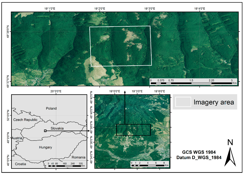
The study site is located within the Kremnica Mountains in the middle of Slovakia (Figure 1) and is a part of the University Forest Enterprise of Technical University in Zvolen. Windthrow Žofia hit the site on 15 May 2014. It is considered the second largest windthrow in the last 20 years with a damaged volume of 4,072,279 m3 [6]. The forest stands that cover the study site consist mainly of European beech (Fagus sylvatica, L.), European silver fir (Abies alba, L.) and Sessile oak (Quercus petraea, L.). The whole study site area covers approximately 200 hectares and intersects 40 forest stands. The size of the site was estimated based on the UAS capability used to acquire imagery during one flight, while the location was chosen with regards to capturing at least two separate windthrow outbreaks.
2.2. Reference Data
Five separate windthrow areas were identified during the terrestrial survey within the study site. The areas were measured by four different GNSS devices in December 2016. Two mapping-grade GNSS devices: Trimble GeoExplorer 6000 (Trimble, Sunnyvale, CA, USA), Trimble Nomad 900 (Trimble, Sunnyvale, CA, USA), and a recreational-grade Garmin 60CS device (Garmin, Olathe, KC, USA) were used. The fourth device was the Sony Xperia X smartphone (Sony, Tokyo, Japan). The operator held the mentioned devices and walked along the border of the disaster areas. Data from all devices were exported to shapefiles. The Trimble GeoExplorer 6000 and Trimble Nomad 900 were the main devices used to determine the windthrow areas. The Garmin 60CS and Sony Xperia X devices were used to test their ability to compete with mapping-grade GNSS devices. We focused on areas that were larger than 0.3 ha. The size is based on Slovak legislation [33] which states that the smallest area for registration as a clear-felled area within the forest and of suitable age for reproduction cutting is 0.3 ha.
The borders of the windthrow areas as measured by the four GNSS devices were processed within the ArcGIS for Desktop software (Environmental Systems Research Institute (ESRI), Redlands, CA, USA [34]). During the processing, the borderlines were generalized and self-intersections of trajectories were removed. This issue was solved by manual editing with an emphasis on changing the polygon area as little as possible. When polygons were made, the areas were tested using one sample t-test to determine if some areas were statistically different from the average value. Each of the five disaster areas was tested separately. If the alternative hypothesis was confirmed, then the results from the device were not used in the following steps. Polygons from all devices for each windthrow area were then overlaid. A new line was manually drawn to create the most accurate border of the disaster areas. The final step was editing the areas due to the time difference. A few tree cuttings on the borders of the windthrow areas were made between the UAS flight (December 2014) and the GNSS measurements (December 2016). These parts were deleted from the GNSS areas. These spots were identified based on photo documentation from the field that was taken during the GNSS measurements, and the documentation was taken from the Budča forest administration.
The reference data for the salvage logging volume of the forest stands within the target area (200 ha) were provided by the Budča forest administration. Every tree felled by the windthrow was harvested and measured during the years 2014 and 2015. The diameter at the middle of the trunk and length of the trunk were measured. The volume of the tree was then derived by using the Hubert cubic formula [35]. The Budča forest administration provided the data about the volume of salvage logging for all forest stands within the study area for all tree species.
2.3. Unmanned Aircraft System Acquisition and Processing
A fixed wing UAS was used for the imagery. The flight was conducted on 9 December 2014. A Gatewing X100 (Trimble, Sunnyvale, CA, USA) with a Ricoh GR Digital 3 camera, (Ricoh imaging company, Tokyo, Japan) which has sensor size of 1/1.7 inch (7.6 mm × 5.7 mm) and a resolution of 10 megapixels was used. The UAS weight was 2.2 kg and had a 1 m wingspan. The flight time was approximately 45 min due to battery life. It was controlled by the base station on the ground.
Before the flight, an open area must be found for take-off and landing. It is recommended that this area should be at least 150 m × 30 m. The flight preparation in the field took approximately 30 min. Before the flight, six ground control points (GCP) were placed within the area and all points were measured by a Stonex S9 GNSS device (Stonex, Lissone, Italy). The number of GCPs is supported by previous research of the authors [36]. These GCPs were used for georeferencing of the point cloud and orthomosaic. Establishing the GCPs took approximately 1 h.
Altogether 19 strips were done during the flight, and 306 images of the target area were taken. The forward and lateral overlap between images was 70%. The last strip was cancelled in the middle of the flight due to low battery warning. The whole flight lasted approximately 48 min from take-off to landing).
The images were processed within the Agisoft Photoscan Professional 1.2.6 software (Agisoft LCC, St. Petersburg, Russia [37]). The software uses a similar algorithm as Scale-invariant feature transform (SIFT) for feature matching within photos. For the camera orientation, greedy and bundle-adjustment algorithms were used. The alignment settings were the maximum number of key and tie points per image. We used the limitless setting for both the original size of images and the pair preselection for every possible pair of all images. With these settings, the highest number of images were correctly aligned at 255 of 306 images. The result was a tie-point cloud that is made from the valid correspondences. A dense point cloud was generated based on the alignment. High quality and aggressive depth filtering settings were used.
The next step was to georeference the point clouds based on the six GCPs. Points were localised and placed on at least three images. All six points were successfully located on the images. The Agisoft Photoscan calculates the root mean square error (RMSE) of the control points, separately for each axis: X as in Equation (1), Y as shown in Equation (2), and Z per Equation (3), and then vertical RMSE in Equation (4) and total RMSE, as shown in Equation (5). We achieved a RSME for the X axis of 0.286 m, 0.337 m for the Y axis, and 0.451 m for the Z axis. The vertical RMSE was 0.442 m, and the total RMSE was 0.631 m.
Derivation of the digital surface and terrain model (DSM and DTM) followed this process using the Module Build DEM for this purpose. DSM was made directly by the module. The module uses the inverse distance weighting (IDW) interpolation method. The input was the dense point cloud. A grid size of 15.7 cm was used by the software for the interpolation purposes, noting it is not possible to edit the grid size. To derive DTM, first we had to classify ground points from the dense point cloud, and then we used Build DEM on these classified ground points to derive DTM. Three parameters were set within the module to classify ground points: maximum angle, maximum distance, and cell size. The maximum angle and distance are two conditions that are checked within the set cell size. The angle and distance of a line were measured between terrain points and a potential point, and if the set parameters were smaller the point was not classified as a ground point and vice versa. This workflow is similar to that followed in [38]. The default settings were used (max. angle 15°; max. distance 1 m; cell size 50 m). The DSM and DTM were exported with a 15-cm pixel size.
To generate the orthomosaic, the module Build Orthomosaic was used. The orthomosaic was based on DSM and a pixel resolution 10 cm was exported. The DSM, DTM, and orthomosaic layers were exported in .tif format.
2.4. Airborne Laser Scanning Acquisition and Processing
Aerial laser scanning data were acquired by a Riegel LMS-Q680i sensor (RIEGL Laser Measurement Systems, Horn, Austria) on 14 April 2012, pre-processed and classified by the external company PHOTOMAP. The sensor operates in near-infrared wavelength with a range accuracy of 2 cm. The whole territory of the University Forest Enterprise was scanned. The mean flight altitude was 700 m above the ground. Minimum scanning density was 5 points/m2. Data was acquired in ETRS-89 datum and transformed to the national coordinate system JTSK03 using 71 ground control points. Noise in the point cloud was removed by automatic filtering and manual editing. Finally, points on the terrain were classified and extracted. The point cloud was divided into standard map sheets with a scale of 1:1000, sized 650 m × 500 m. The ALS processing was done by the Centre of Excellence for Decision Support Systems in Forest and Landscape (ITMS 26220120069), co-funded by the European Regional Development Fund.
The digital terrain model was interpolated from ALS data in ArcGIS for Desktop software. Point clouds were imported into the geographical database. All points representing terrain were stored in a one-point layer. The output point layer covered the entirety of the University Forest Enterprise territory of the Technical University in Zvolen. Due to the enormous amount of data, the DTM was created using tiles with a dimension of 300 m × 250 m. The tiles were processed with an overlap of 10 m to ensure the continuity of DTM. The DTMs were created with a Dealaunay triangulation. The derived irregular network (TIN) was converted into a raster with resolution of 0.5 m. All partial raster layers were merged into an output raster covering the University Forest Enterprise territory.
2.5. Landsat Processing
The Landsat footprint (path188; row26) for the area of interest (AOI) was selected from the WRS-2 map (Worldwide reference system), which is provided by the USGS (United States Geological Survey, Reston, VA, USA [39]). The entire collection of metadata [40] was queried for the selected footprint. The filtering condition for the year was set from 2013 to 2014 to include images before and after the windthrow event. Images from Day of Year (DOY) 70 to 300 were used when the global cloud coverage was defined as being less than 70%.
Landsat 8’s OLI sensor (Operational land imager) started its operational mission phase on 11 April 2013 [41], therefore images with improved radiometric resolution were available when compared those of the older Landsat 7. The AOI is located in the Scan Line Corrector (SLC)–off [42] part on the Landsat 7’s ETM+ sensor. Thus, on Landsat 7 images, blank stripes cover approximately 10% of the AOI.
The Top of Atmosphere (TOA) reflectance was transformed by the USGS Earth Science Processing Architecture (ESPA) service [43] to Bottom of Atmosphere (BOA) reflectance in February 2016. The cloud masks for the images were generated by the Fmask algorithm [44] during the BOA processing.
Image subsets for the AOI were created without resampling, staying in their native UTM34 projection. Only the 30-m resolution bands were used where reflectance could be calculated. The clouds, cloud shadows, and the rest of the image outside the AOI polygon, were masked as no data regions using the Fmask scene classification. For each image, the metadata was stored in a data table which contained the cloud and cloud shadow cover inside the AOI. This table could be used for further manual selection of the proper images. Based on this information, three images were selected from before the windthrow event (May to June 2013) and from after the event (May to beginning of July 2014). In this way, it was guaranteed that all data have similar phenological properties.
The NDVI [45] vegetation index was calculated for all six dates using the near infrared and red band of the Landsat sensors. Despite the two sensors having a difference in bandwidth, which affects the value of vegetation indices, both can be used as complementary data [46]. To reduce noise in the delineated windthrow areas, the three NDVI images before the event were averaged to NDVIbefore, and the three images after the event to NDVIafter. Finally, windthrow areas were derived by applying a threshold (>0.15) to the difference of the averaged NDVI images (NDVIbefore–NDVIafter).
The processing of the imagery was automated by a C-based program, which performed the image selection, cropping, masking, statistic calculation, and product naming, and the OPALS software (TU Wien, Wien, Austria [47]) for delineating the windthrow areas.
2.6. Windthrow Area Identification
Windthrow area identification from UAS imagery was completed within ArcGIS 10.2. First we subtracted DSM from DTM. The subtracted output raster was reclassified to a Boolean raster, where value 1 represents potential windthrow areas and 0 represents non-windthrow areas. Cells with a value of −0.5 and 0.5 were reclassified as value 1 and 0 respectively. The threshold was made based on the analysis of the subtraction map layer. Spots where we assumed conformity between DSM and DTM were analysed to establish the threshold (e.g., roads). This reclassification created a Boolean map of potentially windthrow and non-windthrow areas.
Two types of errors, which we called I and II, occurred. Error I was the labelling of an area as windthrow when it was not. This error occurred in places where the difference between DTM and DSM was within the chosen threshold of −0.5 m to 0.5 m. Error I was caused by two different reasons (A,B): firstly, for reason A, the areas where the DTM and DSM were identical but they were not windthrow areas caused an error. These were, for example, the forest road network, forest gaps, etc. The error was also caused by reason B, an incorrect DSM. In some places, the DTM and DSM were also the same in areas with tree cover. This was caused by insufficient reconstruction of the ground due to the lack of points. Error II occurred when the areas classified as non-windthrow were actually windthrow areas. This error occurred in places where the image alignment was not done properly, and points were missing. To correct this, we manually edited the Boolean raster layer with the ArcScan module. The main goal was to fix all the errors. As a basemap for the decision making, an orthomosaic map from Agisoft Photoscan Professional was used. This step of the data processing was done manually, and we assumed that the different operators would produce different results. Six independent operators did the manual editing and then the results were compared. Three operators were early stage researchers, and three operators were PhD students. All operators were familiar with ArcGIS. Consequently, an overlay of all six operators’ results was completed. Based on the fusion, the best possible border of the damaged areas was drawn with the normalised operators, with emphasis on the operators where at least three of the operators matched one another.
The final step of the data processing was the calculation of the windthrow areas. An edited raster map of the windthrow areas was converted to a feature (polygon) layer. Then this feature layer was intersected with the feature layer of the forest stand map to identify in which forest stands the damaged forest areas were located. The extent of the damage was also determined for each forest stand. A diagram of the whole workflow is shown in Figure 2.
The second method used to identify windthrow areas was combining UAS imagery and airborne laser scanning (the UAS/ALS method). The DTM derived from ALS data was used in the workflow (Figure 2) instead of the DTM from UAS imagery. The other steps in the Agisoft Photoscan workflow remained unchanged. In the case of the ArcGIS workflow, only the threshold parameters within the reclassification step changed from −0.5 m and 0.5 m to −4 m and 4 m. The cells valued at −4 m to 4 m were reclassified to value 0 and 1, respectively. When the UAS imagery was taken many fallen trees were still in the windthrow areas. Furthermore, multiple skid trails were also present. On the other hand, the ALS data collection was made in 2012, when the fallen trees and skid trails, caused by the windthrow, were not present. Therefore, we used the −4 m to 4 m threshold. For this method, errors IB and II occurred, so manual editing was also completed by the same six operators to be able to compare the impact of combining UAS and ALS on the time spent editing and the edited areas. The time period between the editing of the UAS and UAS/ALS data was two months to attempt to reduce the impact of remembering the windthrow areas by the operators.
2.7. Salvage Logging Derivation
The salvage logging calculation from UAS imagery for all tree species within all forest stands was based on the windthrow area identified from UAS imagery and the volume of trees per hectare from the forest management plan. The methodology used to identify windthrow areas from UAS imagery is described in Section 2.6. The identified windthrow areas were assigned to forest stands based on the forest stand map (shapefile). Then, volume per hectare for each tree species was taken from the forest management plans. The plans were provided by the Budča forest administration for all forest stands localized within the study site. All forest management plans were made in 2013. The accuracy of the growing stock estimate is ±15% with 95% confidence [48]. The calculation of the amount of salvage logging for each tree species in all forest stands is shown in Equation (6). The sum of the salvage logging of all tree species within a forests stand is the estimate of salvage logging for each species within the forests stand. The sum of all forest stands’ salvage logging was the whole salvage logging for the study site.
where SL stands for estimated salvage logging, WA is the estimated windthrow area using the UAS method, and Vts is volume of the tree species within the forest stand taken from the forest management plan.
SL = WA * Vts
2.8. Data Interpretation
Four methods were used to map the five windthrow areas. The methods were statistically tested by the Friedman test. We used STATISTICA software (Statsoft Inc., Tulsa, OK, USA [49]). The Friedman test is a nonparametric statistical test, and it is a nonparametric equivalent of parametric repeated measures analysis of variance (ANOVA). The non-parametric Friedman test was used due to the small number of variables. The aim of the statistical testing was to determine whether the methods used are significantly different from each other.
The same Friedman test was also used to determine whether the operators were significantly different from each other when the UAS and UAS/ALS method were used.
Lastly, the GNSS devices were also tested by Friedman test to determine if the devices are significantly different from each other.
When the Friedman test proved a significant difference between methods, operators, or GNSS devices, the Wilcoxon signed-rank test was applied to detect which pairs were significantly different.
Besides the statistical verification, we compared the polygon’s overall matching percentage of the windthrow areas. The Intersect module within ArcGIS was used for all six combinations of methods, and the percentage of the overall match between them and the percentage for every plot was calculated. The overall matching percentage was calculated for four methods, for the different operators (UAS and UAS/ALS methods), and the GNSS devices.
3. Results
The five windthrow areas and extents were successfully identified by all presented methods (UAS, UAS/ALS, and Landsat method), with reference data (GNSS measurements), as shown in Table 1. The sum of the areas varied from 19.8 ha (Landsat) to 25.56 ha (UAS/ALS).
The Friedman test proved the statistically significant difference between methods (p = 0.02627). Then the Wilcoxon signed-rank test confirmed a significant difference between GNSS and Landsat, UAS and Landsat, and UAS/ALS and Landsat (Table 2).
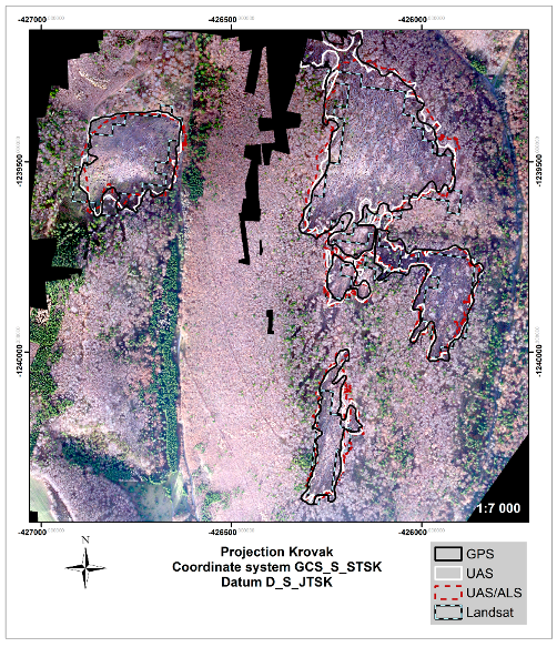
The hypothesis about a significant difference was rejected between GNSS, UAS, and UAS/ALS. The overall matching percentage was 67% and varied in the plots from 56% to 76%. When the Landsat results were excluded, the overall matching percentage was 85% and varied in the plots between 76% and 88%. The borders of all five areas made by all methods are displayed in Figure 3.
The sum of windthrow areas in the entire area, including the small scatter windthrow areas made by all six operators for the UAS method, varied from 26.46 ha to 33.45 ha. When only the five target plots were included, the area ranged from 24.77 ha to 28 ha (Table 3). For the UAS/ALS method, the windthrow areas within the whole area, including the small scatter windthrow areas, varied from 26.35 ha to 32.78 ha, and when only the five target plots were included, the area ranged from 23.89 ha to 27.74 ha between operators. For UAS and UAS/ALS methods, the editing time by operators ranged between 21 min and 33 min, and 7 min and 11 min, respectively. The detailed results of the windthrow areas edited by operators are displayed in Table 3 and Table 4. The Friedman test proved the significant difference between operators within the UAS method (p-value = 0.01282). Within the UAS/ALS method, the hypothesis about differences between operators was rejected (p-value = 0.08027).
The overall matching percentage for operators using the UAS was 82% and varied between 73% and 87% for all plots. The overall matching percentage for the UAS/ALS method was 85% and ranged in the plots from 76% to 98%.
The five areas were mapped by four different GNSS devices. The sum of the areas varied from 25.69 ha to 26.15 ha. Based on the Friedman test results, there was not a significant difference between GNSS devices (p = 0.29158). The area of all the windthrow areas measured by the four devices are shown in Table 5. The overall matching percentage was 88%, and varied between the plots from 76% to 95%.
The areas identified as windthrow, based on the UAS method, intersect with 11 forest stands. The sum of the salvage logging volume measured by the Budča forest administration from the target forest stands, when all trees were included, was 12,380 m3, and the salvage logging volume calculated based on the areas identified from UAS imagery was 13,397 m3. The overall relative difference was 8.2% (−1017 m3). When only the most represented tree species within the forest stands were compared, the salvage logging from the forest administration was 10,648 m3, and from the UAS imagery was 11,173 m3 which is an overall relative difference of 4.93% (525 m3). Results for each forest stand for the most represented tree species are shown in Table 6.
4. Discussion
The windthrow areas were successfully identified within the forest land in the study site from both the UAS and UAS/ALS methods. There was no significant difference between the results and the reference data from the GNSS field measurements that are currently used in forestry on an operational level. The UAS and UAS/ALS methods performed substantially better than Landsat in identifying windthrow disturbances in our study site.
When the UAS method was used, the areas found through operator editing were significantly different. The hypothesis about the existence of a statistical difference between the operators was rejected when the UAS/ALS combination was used. We assume that the UAS/ALS method improved the conformity of the potential windthrow areas layer between operators. Furthermore, the time spent editing decreases almost twofold when the UAS/ALS combination was used. This was mainly caused by error IB, which occurred when the UAS method was used. This error was caused by inaccurate DTM generation derived from UAS imagery. When the ALS point cloud was used, the DTM was correct (Figure 4). The extent of potential windthrow areas before the editing (fully-automatic) was 109.29 ha for the UAS method and 43.28 ha for the UAS/ALS method. This was the main cause of the difference in editing time between the UAS and UAS/ALS methods. The imagery of the area was acquired in the leaf-off season; nevertheless, we were still not able to reconstruct the DTM properly under the forest canopy using the UAS method. ALS has the ability to reconstruct the ground of the forest cover areas in situations where it is not possible to reconstruct it from aerial or UAS imagery due to vegetation cover [50,51,52]. Therefore, it is strongly recommended that ALS should be used for DTM generation, if it is available. If no ALS data is available, it is possible to use UAS imagery alone to successfully detect the affected areas after a windthrow event within forest land.
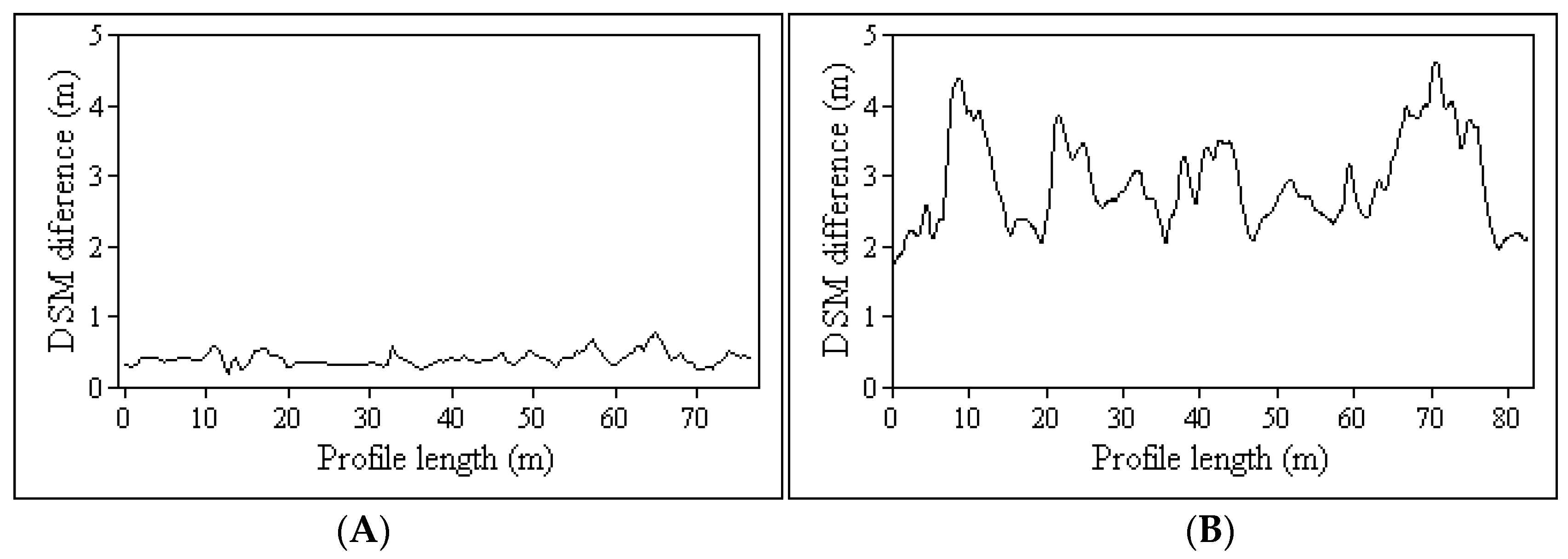
The UAS imagery was acquired almost seven months after the windthrow. However, in almost all target plots there were still downed trees. This influenced the reclassification of the raster layer made from the UAS DSM and ALS DTM subtraction. Within the subtraction raster layer, we established 50 m by 50 m polygons in the middle of each target plot and calculated the maximum and minimum values. The range of the differences varied between −2 m and almost 6 m. The negative values were mainly caused by skid trails in areas where the salvage logging had started. The positive values were caused by laying trees left within the plots. Figure 5 shows examples of elevation profiles from forest roads and the middle of the windthrow plot. We can clearly see the difference, caused by the trees laying within the disaster area.
A prior study also used the combination of UAS imagery and ALS to identify the regeneration processes of vegetation within the forest land after forest fire disturbance [53]. They successfully identified all the main changes within the area as aspen regeneration or snag falls and logging activities. They proved, as is also proven in this study, the ability to combine different years (2008 and 2015 [53]) of UAS imagery with ALS for the same area.
The other advantage of using UAS imagery is the ability to achieve a high resolution orthophoto map, down to a few centimetres, which makes it possible to identify small open areas within a forest. In some cases, it is not feasible to determine these spots during field mapping by GNSS, especially in cases when there are multiple spots within the area, and forest operators are busy handling the large damaged areas. In our case, we were able to detect the areas under 0.3 ha (Figure 6). The sum of these small windthrow areas was 2.28 ha. The average volume per hectare of the most represented tree species within the intersected forest stands was 350 m3. We can then assume that the salvage logging of the most represented tree species was approximately 798 m3. The ability to map small open areas within forest stands was also reported by [31]. The authors were able to identify crown gaps as small as 1 m2 using UAS imagery. On the contrary, recreational-grade and smartphone GNSS receivers have been reported to have difficulties with areas smaller than 0.5 ha [12].
We also estimated the salvage logging volume within the study site. Our estimate was based on the estimated windthrow areas from UAS imagery and on the per hectare volumes of every tree species from a forest management plan. The plan was last updated in 2013. The volume was calculated with 15% accuracy at a 95% confidence level. The estimated volume was compared to actual salvage logging measured by the Budča forest administration. They used the Huber cubic formula [35] to calculate the volume of fallen trees based on the diameter at the middle of the trunk and length of the trunk. According to [54], this method slightly overestimates the volume of trees. Also, other errors should be taken into account. The most important error is the random error from tree measurement with the Hubert cubic formula method, but the measurements from the forest management plans can also have an immense impact on the calculations.
As mentioned, the overall relative error of the salvage logging estimate was 4.93%. However, the relative overall error of salvage logging for each forest stand ranged from 100% to −235% and the estimate errors in cubic meters varied from −624 m3 to 435 m3. One of the sources of this variability was caused, in our opinion, by inaccurate determination of forest stand boundaries by foresters during harvesting and trees were incorrectly assigned to a neighbouring forest stand. The overall relative error supports the theory. The goal of salvage logging estimation is to provide a first approximation immediately after the windthrow to give an understanding of the windthrow scale. In practice, the ocular method is used. The precision of the estimate using this method depends greatly on the forester and his experience.
The UAS Gatewing X100 captured 306 images altogether, and we were able to align 255 images. Even if we used different settings for the alignment and different software (Pix4D mapper, version 3.1.23, (Pix4D SA, Lausanne, Switzerland)), we were not able to align all the images. Due to this, the point cloud had gaps within the area, and DTM and DSM were not properly generated. These gaps were situated on the hilly sites. The longitudinal and lateral overlap was set to 70% by the operator. This means that the UAS had overlap for the images in an area that have the same altitude as the starting point. The areas located at higher altitude have smaller overlaps and vice versa. From our perspective, the imagery obtained by fixed wing UAS should be done with a longitudinal overlap of 80–90% and a lateral overlap of at least of 60–70%. When the overlap is increased, a smaller area will be mapped, but ensuring the ability to align all the images is of higher priority.
The UAS imagery has the advantage to be used immediately after the windthrow event, plus the clouds do not affecting the imagery as with aerial or satellite imagery [31,53]. However, right after the wind event, the foresters do not know where the damaged forest areas are, and the imagery should be done for the entire forest area managed by the local forest administration. Altogether 8212 ha of forest land is managed by the Budča forest administration, where our site was situated. We used the eMotion 2.4.13 software (SenseFly SA, Cheseaux-sur-Lausanne, Switzerland) to simulate flights of fixed-wing UAS Ebee RTK (SenseFly SA, Cheseaux-sur-Lausanne, Switzerland) with a G9X RGB camera (Canon, Tokyo, Japan). The longitudinal overlap was set to 85% and lateral to 60%. We also set the wind speed to 4 m/s. With these settings, the UAS can cover approximately 200 ha per flight to achieve 10 cm resolution for the orthomosaic. To acquire imagery of the whole area approximately 60 flights are needed taking into account the shape of the area of the forest stands. As the operator is capable of doing six flights per day, the imagery should take ten days for this area.
5. Conclusions
This study focuses on the capabilities of unmanned aircraft systems (UAS) to estimate the forest areas affected after windthrow and the volume of salvage logging. Furthermore, the combination of UAS photogrammetry and airborne laser scanning (UAS/ALS) was investigated. For reference data, the windthrow areas were mapped by four different global navigation satellite system (GNSS) devices and was also estimated using Landsat imagery. Data about the volume of salvage logging were taken from the Budča forest district administration for comparison with the estimated volume of salvage logging obtained from the UAS.
The windthrow areas were successfully identified using a semi-automatic approach within the forest land of the study site with both the UAS and UAS/ALS methods. There was no significant difference between the results and the GNSS field measurements that are currently used in forestry at the operational level. On the other hand, the results from the Landsat imagery significantly underestimated the areas in comparison to GNSS, and the UAS and UAS/ALS methods. The difference between the salvage logging volume of the most represented tree species within the forest stands estimated from UAS and the volume provided by the forest district administration was 4.93%. The results from UAS overestimated the volume provided by the forest district administration.
Acknowledgments
This work was supported by the Slovak Research and Development Agency under the grant No. APVV-15-0714: “Mitigation of climate change risk by optimization of forest harvesting scheduling”, and by the Slovak Research and Development Agency grant No. APVV-0069-12: “New technology of nature management (NEWTON)”. The authors would like to thank to SGS Holding for the data acquisition by the Gatewing X100.
Author Contributions
All authors contributed to the writing of the initial manuscript; Martin Mokroš, Jozef Výbošťok and Ján Merganič contributed to the initial proposal of methodology; Martin Mokroš processed the UAS data and conducted the analyses; Martin Mokroš and Jozef Výbošťok wrote the initial draft of the manuscript; Jozef Výbošťok, Ján Merganič and Julián Tomaštík surveyed the reference data; Markus Hollaus and Iván Barton processed the Landsat data; Milan Koreň processed the airborne laser scanning data; Juraj Čerňava processed the GNSS data.
Conflicts of Interest
The authors declare no conflicts of interest.
References
- Gilliam, F.S. The Herbaceous Layer in Forests of Eastern North America; Oxford University Press: New York, NY, USA, 2014. [Google Scholar]
- Gardiner, B.; Blennow, K.; Carnus, J.M.; Fleischer, P.; Ingemarson, F.; Landman, G.; Lindner, M.; Marzano, M.; Nicoll, B.; Orazio, C.; et al. Destructive Storms in European Forests: Past and Forthcoming Impacts; Final Report to European CommissioneDG Environment; European Forest Institute (EFIATLANTIC): Cestas, France, 2010; p. 138. [Google Scholar]
- Gerendiain, A.Z.; Pukkala, T.; Peltola, H. Effects of wind damage on the optimal management of boreal forests under current and changing climatic conditions. Can. J. For. Res. 2016, 47, 246–256. [Google Scholar] [CrossRef]
- Schelhaas, M.J.; Nabuurs, G.J.; Schuck, A. Natural disturbances in the European forests in the 19th and 20th centuries. Glob. Chang. Biol. 2003, 9, 1620–1633. [Google Scholar] [CrossRef]
- Falťan, V.; Katina, S.; Bánovský, M.; Pazúrová, Z. The influence of site conditions on the impact of windstorms on forests: The case of the high tatras foothills (Slovakia) in 2004. Morav. Geogr. Rep. 2009, 17, 10–18. [Google Scholar]
- Kunca, A.; Leontovič, R.; Galko, J.; Zúbrik, M.; Vakula, J.; Gubka, A.; Nikolov, C.; Rell, S.; Longauerová, V.; Maľová, M.; et al. Windthrow žofia from May 15, 2014 in Slovak forests and suggested control measures. In Dendrologické dni v Arboréte Mlyňany SAV 2014; Arborétum Mlyňany: Vieska nad Žitavou, Slovakia, 2014; pp. 105–112. [Google Scholar]
- Schelhaas, M.J.; Hengeveld, G.; Moriondo, M.; Reinds, G.J.; Kundzewicz, Z.W.; Ter Maat, H.; Bindi, M. Assessing risk and adaptation options to fires and windstorms in European forestry. Mitig. Adapt. Strateg. Glob. Chang. 2010, 15, 681–701. [Google Scholar] [CrossRef]
- Seidl, R.; Thom, D.; Kautz, M.; Martin-Benito, D.; Peltoniemi, M.; Vacchiano, G.; Wild, J.; Ascoli, D.; Petr, M.; Honkaniemi, J.; et al. Forest disturbances under climate change. Nat. Clim. Chang. 2017, 7, 395–402. [Google Scholar] [CrossRef]
- Seidl, R.; Schelhaas, M.J.; Lexer, M.J. Unraveling the drivers of intensifying forest disturbance regimes in Europe. Glob. Chang. Biol. 2011, 17, 2842–2852. [Google Scholar] [CrossRef]
- Böhm, P. Sturmschäden in Schwaben von 1950 bis 1980. Allg. Forstz. 1981, 36, 1380. [Google Scholar]
- Koloman, P.; Střelec, L. Time minimizing transportation of calamity fallen timber. AIP Conf. Proc. 2013, 1558, 1843–1846. [Google Scholar]
- Tomaštík, J.; Tomaštík, J.; Saloň, Š.; Piroh, R. Horizontal accuracy and applicability of smartphone GNSS positioning in forests. Forestry 2016, 90, 187–198. [Google Scholar] [CrossRef]
- Alberts, K. Landsat Data Characteristics and Holdings; A Presentation of USGS Landsat Ground System Lead; U.S. Geological Survey (USGS): Reston, VA, USA, 2012.
- Havašová, M.; Ferenčík, J.; Jakuš, R. Interactions between windthrow, bark beetles and forest management in the Tatra national parks. For. Ecol. Manag. 2017, 391, 349–361. [Google Scholar] [CrossRef]
- Schroeder, T.A.; Wulder, M.A.; Healey, S.P.; Moisen, G.G. Mapping wild fi re and clearcut harvest disturbances in boreal forests with Landsat time series data. Remote Sens. Environ. 2011, 115, 1421–1433. [Google Scholar] [CrossRef]
- Franklin, S.E.; Moskal, L.M.; Lavigne, M.B.; Pugh, K. Interpretation and classification of partially harvested forest stands in the Fundy model forest using multitemporal Landsat TM digital data. Can. J. Remote Sens. 2000, 26, 318–333. [Google Scholar] [CrossRef]
- Cohen, W.B.; Yang, Z.; Stehman, S.V.; Schroeder, T.A.; Bell, D.M.; Masek, J.G.; Huang, C.; Meigs, G.W. Forest disturbance across the conterminous United States from 1985–2012: The emerging dominance of forest decline. For. Ecol. Manag. 2016, 360, 242–252. [Google Scholar] [CrossRef]
- Pflugmache, D.; Cohen, W.B.; Kennedy, R.E. Using Landsat-derived disturbance history (1972–2010) to predict current forest structure. Remote Sens. Environ. 2012, 122, 146–165. [Google Scholar] [CrossRef]
- Kennedy, R.E.; Yang, Z.; Cohen, W.B. Detecting trends in forest disturbance and recovery using yearly Landsat time series: 1. LandTrendr—Temporal segmentation algorithms. Remote Sens. Environ. 2010, 114, 2897–2910. [Google Scholar] [CrossRef]
- Tang, L.; Shao, G. Drone remote sensing for forestry research and practices. J. For. Res. 2015, 26, 791–797. [Google Scholar] [CrossRef]
- Wulder, M.A.; Dymond, C.C.; White, J.C.; Leckie, D.G.; Carroll, A.L. Surveying mountain pine beetle damage of forests: A review of remote sensing opportunities. For. Ecol. Manag. 2006, 221, 27–41. [Google Scholar] [CrossRef]
- Arroyo, L.A.; Pascual, C.; Manzanera, J.A. Fire models and methods to map fuel types: The role of remote sensing. For. Ecol. Manag. 2008, 256, 1239–1252. [Google Scholar] [CrossRef] [Green Version]
- Immitzer, M.; Vuolo, F.; Atzberger, C. First experience with Sentinel-2 data for crop and tree species classifications in central Europe. Remote Sens. 2016, 8, 166. [Google Scholar] [CrossRef]
- Tran, T.H.G.; Hollaus, M.; Nguyen, B.D.; Pfeifer, N. Assessment of wooded area reduction by airborne laser scanning. Forests 2015, 6, 1613–1627. [Google Scholar] [CrossRef]
- Nyström, M.; Holmgren, J.; Fransson, J.E.S.; Olsson, H. Detection of windthrown trees using airborne laser scanning. Int. J. Appl. Earth Obs. Geoinf. 2014, 30, 21–29. [Google Scholar] [CrossRef]
- Pearson, A.F. Natural and logging disturbances in the temperate rain forests of the Central Coast, British Columbia. Can. J. For. Res. 2010, 40, 1970–1984. [Google Scholar] [CrossRef]
- Whitehead, K.; Hugenholtz, C.H.; Myshak, S.; Brown, O.; LeClair, A.; Tamminga, A.; Barchyn, T.E.; Moorman, B.; Eaton, B. Remote sensing of the environment with small unmanned aircraft systems (UASs), part 2: Scientific and commercial applications. J. Unmanned Veh. Syst. 2014, 2, 86–102. [Google Scholar] [CrossRef]
- Yuan, C.; Zhang, Y.; Liu, Z. A survey on technologies for automatic forest fire monitoring, detection, and fighting using unmanned aerial vehicles and remote sensing techniques. Can. J. For. Res. 2015, 45, 783–792. [Google Scholar] [CrossRef]
- Näsi, R.; Honkavaara, E.; Lyytikäinen-Saarenmaa, P.; Blomqvist, M.; Litkey, P.; Hakala, T.; Viljanen, N.; Kantola, T.; Tanhuanpää, T.; Holopainen, M. Using UAV-Based Photogrammetry and Hyperspectral Imaging for Mapping Bark Beetle Damage at Tree-Level. Remote Sens. 2015, 7, 15467–15493. [Google Scholar] [CrossRef]
- Watts, A.C.; Ambrosia, V.G.; Hinkley, E.A. Unmanned aircraft systems in remote sensing and scientific research: Classification and considerations of use. Remote Sens. 2012, 4, 1671–1692. [Google Scholar] [CrossRef]
- Getzin, S.; Nuske, R.S.; Wiegand, K. Using unmanned aerial vehicles (UAV) to quantify spatial gap patterns in forests. Remote Sens. 2014, 6, 6988–7004. [Google Scholar] [CrossRef]
- Vaudour, E.; Leclercq, L.; Gilliot, J.M.; Chaignon, B. Retrospective 70 y-spatial analysis of repeated vine mortality patterns using ancient aerial time series, Pléiades images and multi-source spatial and field data. Int. J. Appl. Earth Obs. Geoinf. 2017, 58, 234–248. [Google Scholar] [CrossRef]
- Vyhláška Ministerstva Pôdohospodárstva a Rozvoja Vidieka Slovenskej Republiky zo 7. Septembra 2011 o Lesnej Hospodárskej Evidencii; Predpis č. 297/2011, Z. z.; Ministerstva Pôdohospodárstva a Rozvoja Vidieka Slovenskej Republiky: Bratislava, Slovakia, 2011.
- ArcGIS Software Version 10.2. Available online: http://support.esri.com/Products/Desktop/arcgis-desktop/arcmap/10-2-2 (accessed on 29 May 2017).
- Huber, F.X. Hilfstabellen für Bedienstete des Forst und Baufachs und auch für Ökonomen zur Leichten und Schnellen Bestimmung des Massengehaltes Roher; Fleischmann: München, Germany, 1828. [Google Scholar]
- Tomaštik, J.; Mokroš, M.; Saloň, Š.; Chudý, F.; Tunák, D. Accuracy of Photogrammetric UAV-Based Point Clouds under Conditions of Partially-Open Forest Canopy. Forests 2017, 8, 151. [Google Scholar] [CrossRef]
- AgiSoft Software Version 1.2.6. Available online: http://www.agisoft.com/downloads/installer/ (accessed on 29 May 2017).
- Axelsson, P. DEM generation from laser scanner data using adaptive TIN models. Int. Arch. Photogramm. Remote Sens. 2000, 33, 111–118. [Google Scholar]
- United States Geological Survey (USGS). WRS-1 and WRS-2 Shapefiles. Available online: https://landsat.usgs.gov/pathrow-shapefiles (accessed on 24 November 2016).
- United States Geological Survey (USGS). Landsat Collection of Metada. Available online: https://landsat.usgs.gov/download-entire-collection-metadata (accessed on 24 November 2016).
- United States Geological Survey (USGS). Landsat 8. Available online: https://landsat.usgs.gov/landsat-8-history (accessed on 24 November 2016).
- Markham, B.L.; Storey, J.C.; Williams, D.L.; Irons, J.R. Landsat sensor performance: History and current status. IEEE Trans. Geosci. Remote Sens. 2004, 42, 2691–2694. [Google Scholar] [CrossRef]
- United States Geological Survey (USGS). USGS ESPA Service. Available online: https://espa.cr.usgs.gov/ (accessed on 24 November 2016).
- Zhu, Z.; Woodcock, C.E. Object-based cloud and cloud shadow detection in Landsat imagery. Remote Sens. Environ. 2012, 118, 83–94. [Google Scholar] [CrossRef]
- Tucker, C.J.; Slayback, D.A.; Pinzon, J.E.; Los, S.O.; Myneni, R.B.; Taylor, M.G. Higher northern latitude normalized difference vegetation index and growing season trends from 1982 to 1999. Int. J. Biometeorol. 2001, 45, 184–190. [Google Scholar] [CrossRef] [PubMed]
- Li, P.; Jiang, L.; Feng, Z. Cross-comparison of vegetation indices derived from landsat-7 enhanced thematic mapper plus (ETM+) and landsat-8 operational land imager (OLI) sensors. Remote Sens. 2013, 6, 310–329. [Google Scholar] [CrossRef]
- Pfeifer, N.; Mandlburger, G.; Otepka, J.; Karel, W. OPALS—A framework for Airborne Laser Scanning data analysis. Comput. Environ. Urban Syst. 2014, 45, 125–136. [Google Scholar] [CrossRef]
- Bavlšík, J.; Antal, P.; Kočik, L.; Kominka, V.; Kučera, J.; Machanský, M. Pracovné Postupy Hospodárskej Úpravy Lesov; Národné Lesnícke Centrum: Zvolen, Slovakia, 2008. [Google Scholar]
- StatSoft, Inc. STATISTICA (Data Analysis Software System). Version 12. 2011. Available online: www.statsoft.com (accessed on 10 November 2016).
- Baltsavias, E.P. A comparison between photogrammetry and laser scanning. ISPRS J. Photogramm. Remote Sens. 1999, 54, 83–94. [Google Scholar] [CrossRef]
- White, J.C.; Stepper, C.; Tompalski, P.; Coops, N.C.; Wulder, M.A. Comparing ALS and image-based point cloud metrics and modelled forest inventory attributes in a complex coastal forest environment. Forests 2015, 6, 3704–3732. [Google Scholar] [CrossRef]
- Hsieh, Y.C.; Chan, Y.C.; Hu, J.C. Digital elevation model differencing and error estimation from multiple sources: A case study from the Meiyuan Shan landslide in Taiwan. Remote Sens. 2016, 8, 199. [Google Scholar] [CrossRef]
- Aicardi, I.; Garbarino, M.; Lingua, A.; Lingua, E.; Marzano, R.; Piras, M. Monitoring Post-Fire Forest Recovery Using Multi-Temporal Digital Surface Models Generated From. EARSeL eProc. 2016, 15, 1–8. [Google Scholar]
- Šmelko, Š.; Scheer, Ľ.; Petráš, R.; Ďurský, J.; Fabrika, M. Meranie Lesa a Dreva; Ústav pre Výchovu a Vzdelávanie Pracovníkov Lesného Hospodárstva: Zvolen, Slovakia, 2003. [Google Scholar]
Figure 1.
Map of the study site situated in the middle of Slovakia. The white rectangle represents the outlines of the unmanned aircraft systems (UAS) imagery.
Figure 1.
Map of the study site situated in the middle of Slovakia. The white rectangle represents the outlines of the unmanned aircraft systems (UAS) imagery.

Figure 2.
The workflow diagram of the imagery data processing to the final area and volume estimation conducted within the Agisoft Photoscan software [37] and ArcGIS 10.2 software [34].
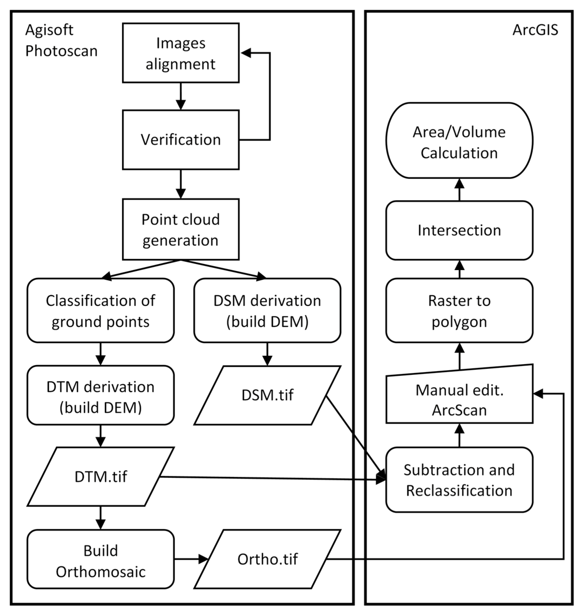
Figure 3.
View of the windthrow areas determined by all four presented methods overlaid on the orthomosaic derived from UAS imagery.
Figure 3.
View of the windthrow areas determined by all four presented methods overlaid on the orthomosaic derived from UAS imagery.

Figure 4.
An example of the potential windthrow areas detected by the UAS method and UAS/ALS methods with emphasis on error 1B which is only present with the UAS method.
Figure 4.
An example of the potential windthrow areas detected by the UAS method and UAS/ALS methods with emphasis on error 1B which is only present with the UAS method.
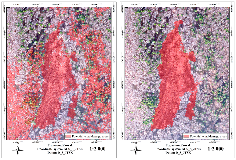
Figure 5.
Road profile (A) and calamity profile (B) comparison between the of UAS DSM and UAS/ALS DTM maps.
Figure 5.
Road profile (A) and calamity profile (B) comparison between the of UAS DSM and UAS/ALS DTM maps.

Figure 6.
The view of the windthrow areas under <0.3 ha detected within the area from UAS imagery.


Table 1.
Summary of the windthrow areas identified by all methods and reference data used from global navigation satellite system (GNSS) measurements. UAS, unmanned aircraft systems; ALS, airborne laser scanning.
Table 1.
Summary of the windthrow areas identified by all methods and reference data used from global navigation satellite system (GNSS) measurements. UAS, unmanned aircraft systems; ALS, airborne laser scanning.
| Plot ID | GNSS | UAS | UAS/ALS | Landsat |
|---|---|---|---|---|
| (ha) | ||||
| 1 | 5.29 | 5.38 | 5.08 | 4.59 |
| 2 | 2.44 | 2.48 | 2.78 | 1.71 |
| 3 | 0.75 | 0.89 | 1.03 | 0.45 |
| 4 | 4.32 | 4.10 | 4.04 | 3.42 |
| 5 | 12.59 | 12.24 | 12.63 | 9.63 |
| Sum | 25.39 | 25.09 | 25.56 | 19.8 |
Table 2.
The p-values of the Wilcoxon paired test for used methods and GNSS measurements.
| GNSS | UAS | UAS/ALS | |
|---|---|---|---|
| UAS | 0.6858 | - | - |
| UAS/ALS | 0.6858 | 0.3452 | - |
| Landsat | 0.0431 | 0.0431 | 0.0431 |
Table 3.
Comparison of edited windthrow areas and editing time of operators using the UAS method.
| Plot ID | Operator ID | |||||
|---|---|---|---|---|---|---|
| 1 | 2 | 3 | 4 | 5 | 6 | |
| (ha) | ||||||
| 1 | 5.23 | 4.84 | 4.7 | 5.23 | 5.24 | 5.29 |
| 2 | 2.68 | 2.81 | 2.69 | 2.66 | 3.39 | 2.78 |
| 3 | 1.02 | 1.18 | 1.07 | 1.06 | 1.4 | 1.16 |
| 4 | 3.81 | 3.93 | 3.95 | 3.98 | 5 | 4.2 |
| 5 | 12.49 | 12.01 | 12.48 | 12.95 | 12.97 | 12.94 |
| Sum | 25.23 | 24.77 | 24.89 | 25.88 | 28 | 26.37 |
| Editing time (min) | 25 | 21 | 30 | 19 | 33 | 26 |
Table 4.
Comparison of edited windthrow areas and editing time of operators when using the UAS/ALS method.
Table 4.
Comparison of edited windthrow areas and editing time of operators when using the UAS/ALS method.
| Plot ID | Operator ID | |||||
|---|---|---|---|---|---|---|
| 1 | 2 | 3 | 4 | 5 | 6 | |
| (ha) | ||||||
| 1 | 5.53 | 4.97 | 5.46 | 5.61 | 4.96 | 4.6 |
| 2 | 2.62 | 2.86 | 2.91 | 2.63 | 2.88 | 2.89 |
| 3 | 1.08 | 1.04 | 1.28 | 1.15 | 1.19 | 0.92 |
| 4 | 3.99 | 4.04 | 4.1 | 4.03 | 4.04 | 4.06 |
| 5 | 12.91 | 12.67 | 13.99 | 13.32 | 13.44 | 11.42 |
| Sum | 26.13 | 25.58 | 27.74 | 26.74 | 26.51 | 23.89 |
| Editing time (min) | 8 | 7 | 14 | 11 | 9 | 8 |
Table 5.
Summary of windthrow areas mapped by the four different GNSS devices.
| Plot ID | GeoXT | Nomad | Garmin | Xperia |
|---|---|---|---|---|
| (ha) | ||||
| 1 | 5.45 | 5.48 | 5.49 | 5.56 |
| 2 | 2.19 | 2.06 | 2.06 | 2.34 |
| 3 | 0.84 | 0.68 | 0.83 | 0.87 |
| 4 | 4.44 | 4.54 | 4.34 | 4.19 |
| 5 | 13.10 | 12.94 | 13.15 | 13.19 |
| Sum | 26.02 | 25.69 | 25.87 | 26.15 |
Table 6.
Volume estimation of salvage logging based on the data from the forest plan and from UAS imagery (FS—Fagus sylvatica; AA—Abies alba; PA—Picea abies).
Table 6.
Volume estimation of salvage logging based on the data from the forest plan and from UAS imagery (FS—Fagus sylvatica; AA—Abies alba; PA—Picea abies).
| Stand ID | Forest Plan (FP) | UAS | Volume Difference FP − UAS (m3 (%)) | ||||
|---|---|---|---|---|---|---|---|
| Tree Species | Tree Species Rep. (%) | Volume Per ha (m3) | Volume of Damaged Trees (m3) | Calamity Area (ha) | Volume of Damaged Trees (m3) | ||
| 541a | FS | 95 | 486 | 2794 | 6.12 | 3418 | −624 (22) |
| 542 | FS | 90 | 430 | 2614 | 5.90 | 2392 | 222 (8) |
| 543 | FS | 80 | 346 | 35 | 0.40 | 109 | −74 (210) |
| 544 | FS | 85 | 411 | 1395 | 3.35 | 1484 | −89 (6) |
| 545 | FS | 55 | 229 | 79 | 0.83 | 187 | −108 (136) |
| 547a | FS | 80 | 464 | 1552 | 2.86 | 1117 | 435 (28) |
| 547b | FS | 75 | 408 | 183 | 1.60 | 614 | −431 (235) |
| 559 | FS | 80 | 325 | 1762 | 6.89 | 1798 | −35 (2) |
| 560a | AA | 88 | 155 | 18 | 0.11 | 0 | 18 (100) |
| 562a | FS | 60 | 220 | 138 | 0.61 | 52 | 86 (62) |
| 562b | PA | 50 | 162 | 78 | 0.00 | 2 | 75 (97) |
| Sum | 10,648 | 11,173 | −525 (4.93) | ||||
© 2017 by the authors. Licensee MDPI, Basel, Switzerland. This article is an open access article distributed under the terms and conditions of the Creative Commons Attribution (CC BY) license (http://creativecommons.org/licenses/by/4.0/).
Share and Cite
MDPI and ACS Style
Mokroš, M.; Výbošťok, J.; Merganič, J.; Hollaus, M.; Barton, I.; Koreň, M.; Tomaštík, J.; Čerňava, J. Early Stage Forest Windthrow Estimation Based on Unmanned Aircraft System Imagery. Forests 2017, 8, 306. https://doi.org/10.3390/f8090306
AMA Style
Mokroš M, Výbošťok J, Merganič J, Hollaus M, Barton I, Koreň M, Tomaštík J, Čerňava J. Early Stage Forest Windthrow Estimation Based on Unmanned Aircraft System Imagery. Forests. 2017; 8(9):306. https://doi.org/10.3390/f8090306
Chicago/Turabian StyleMokroš, Martin, Jozef Výbošťok, Ján Merganič, Markus Hollaus, Iván Barton, Milan Koreň, Julián Tomaštík, and Juraj Čerňava. 2017. "Early Stage Forest Windthrow Estimation Based on Unmanned Aircraft System Imagery" Forests 8, no. 9: 306. https://doi.org/10.3390/f8090306
Note that from the first issue of 2016, this journal uses article numbers instead of page numbers. See further details here.