Spatial Pattern and Temporal Stability of Root-Zone Soil Moisture during Growing Season on a Larch Plantation Hillslope in Northwest China


Abstract
:1. Introduction
2. Materials and Methods
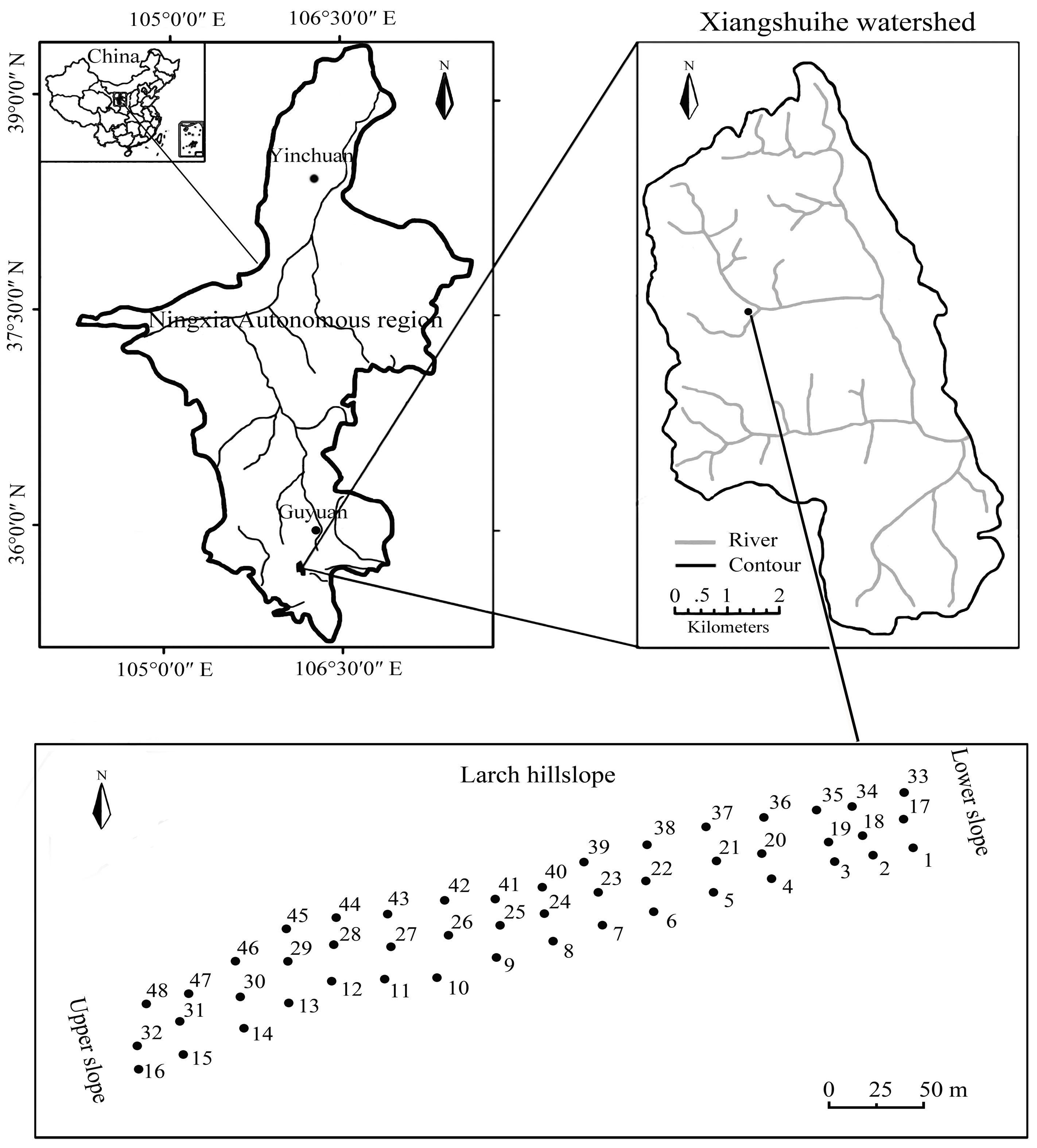
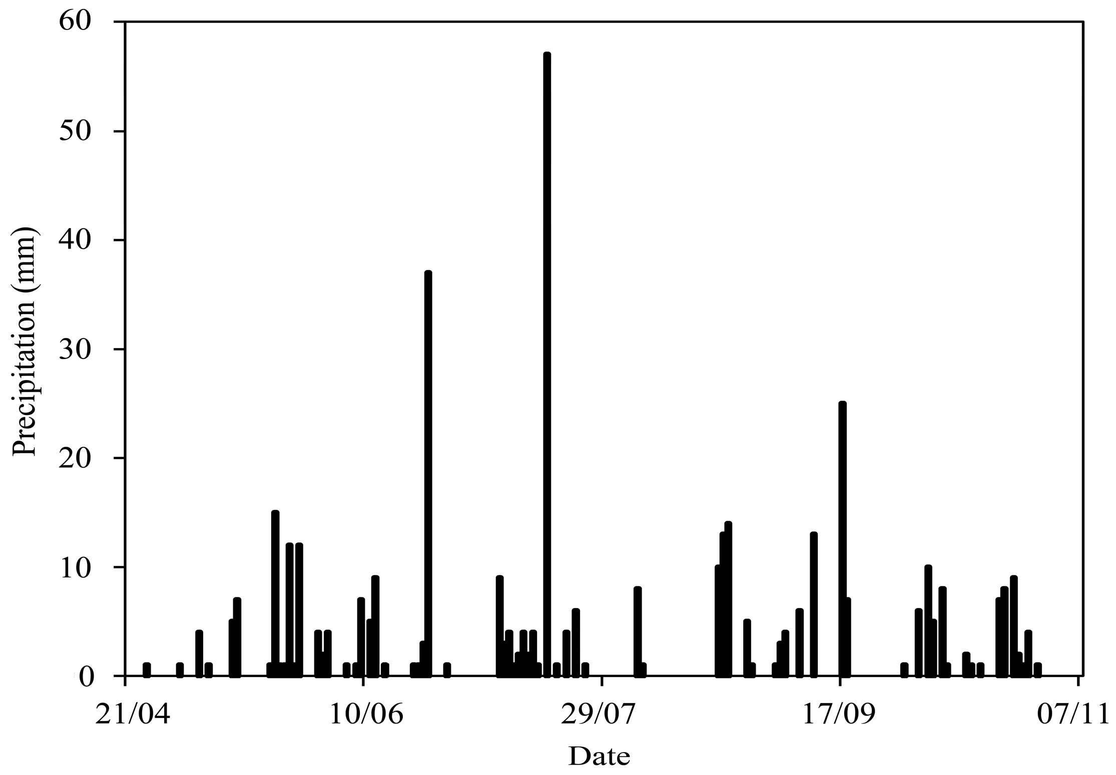
2.1. Study Area
2.2. Sampling Points and Measurement of Soil and Vegetation Properties
2.3. Data Analysis
2.3.1. Spearman’s Rank Correlation Coefficient
2.3.2. Frequency Distribution
2.3.3. Relative Difference Analysis
2.3.4. The Estimation of Slope Mean VSM by Direct and Indirect Methods
2.3.5. Statistical Analysis
3. Results
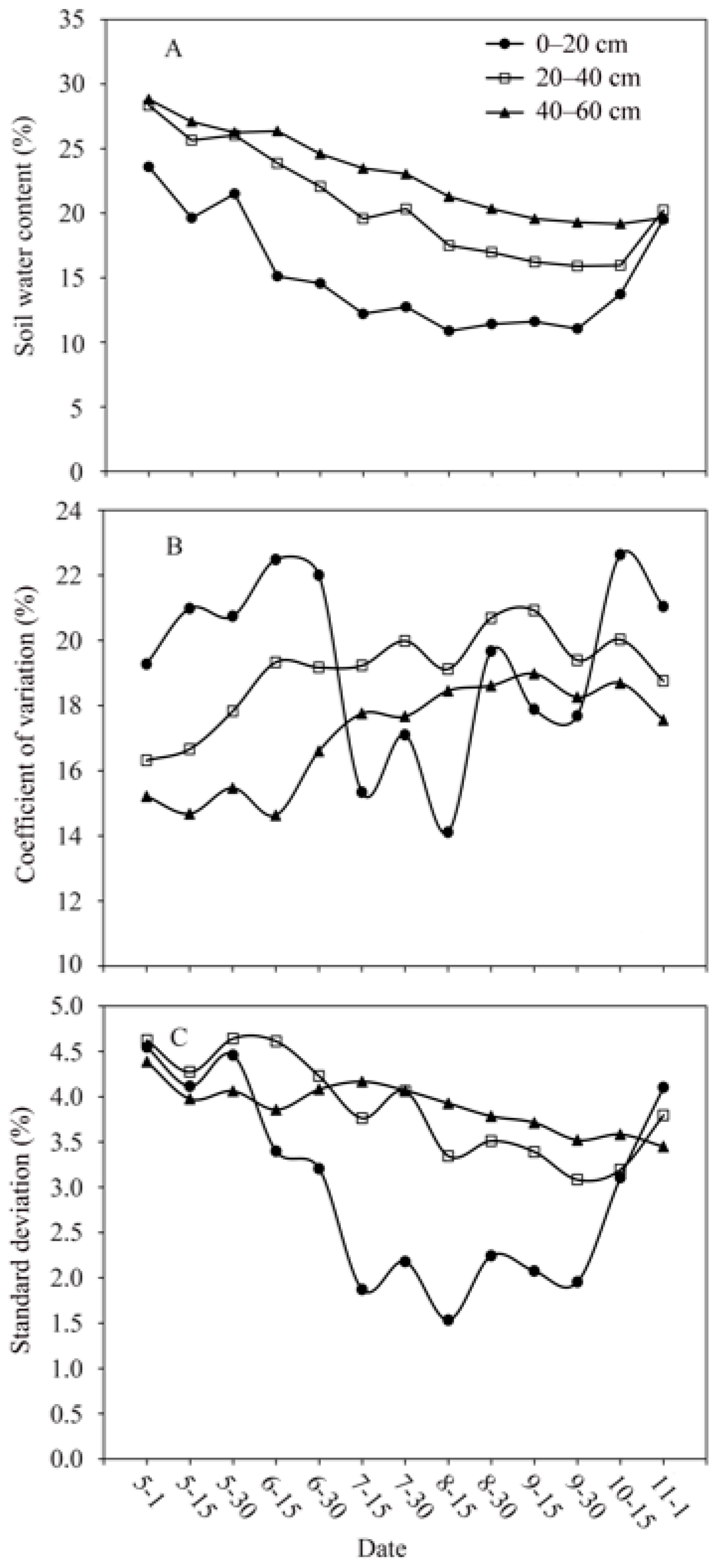
3.1. Spatio-Temporal Variation Analysis of VSM
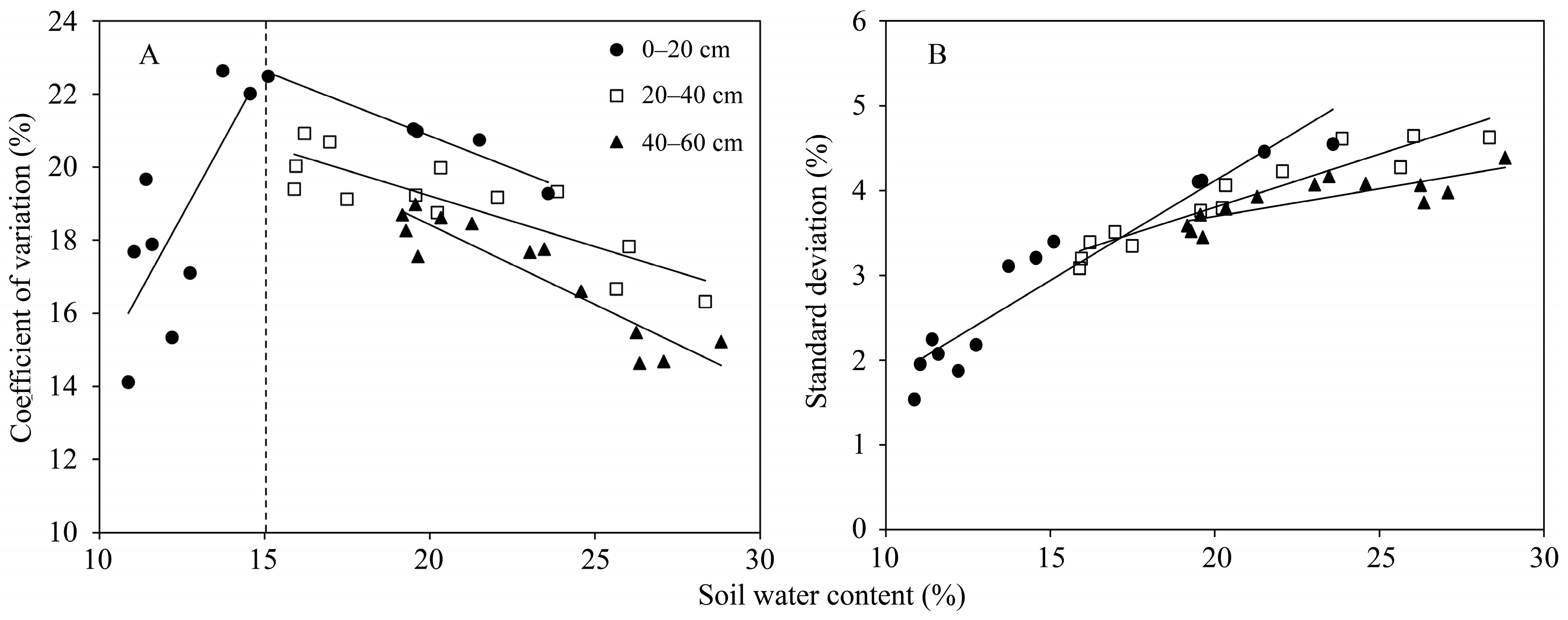
3.2. SDs and CVs versus Slope Mean VSM
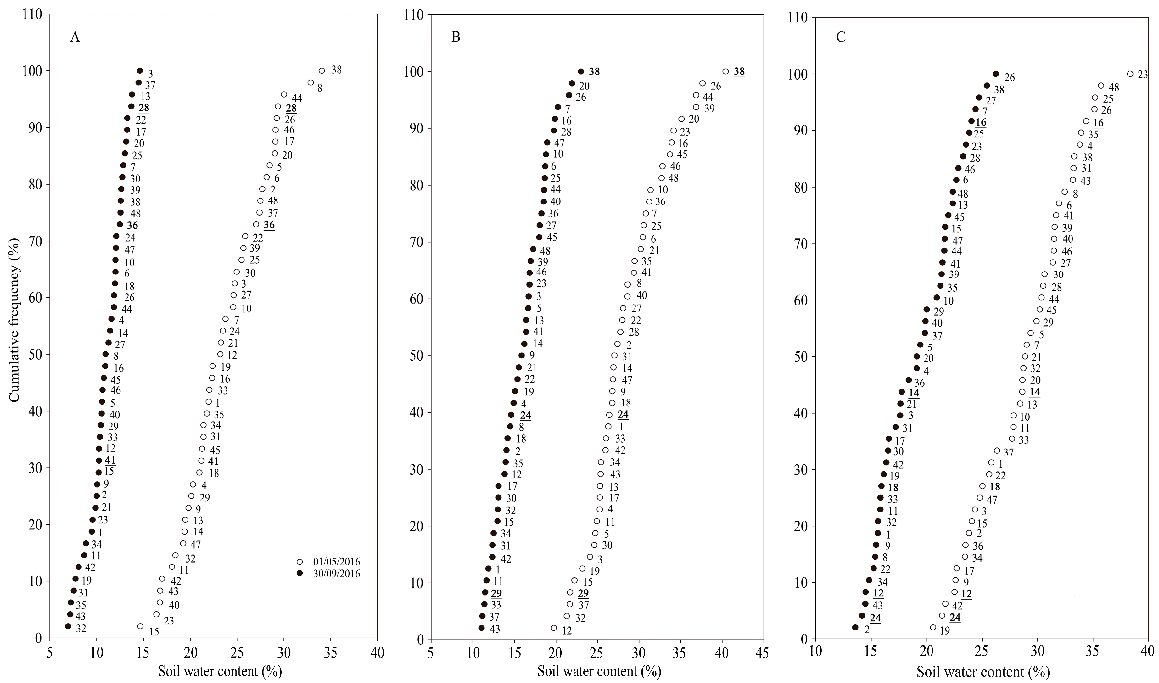
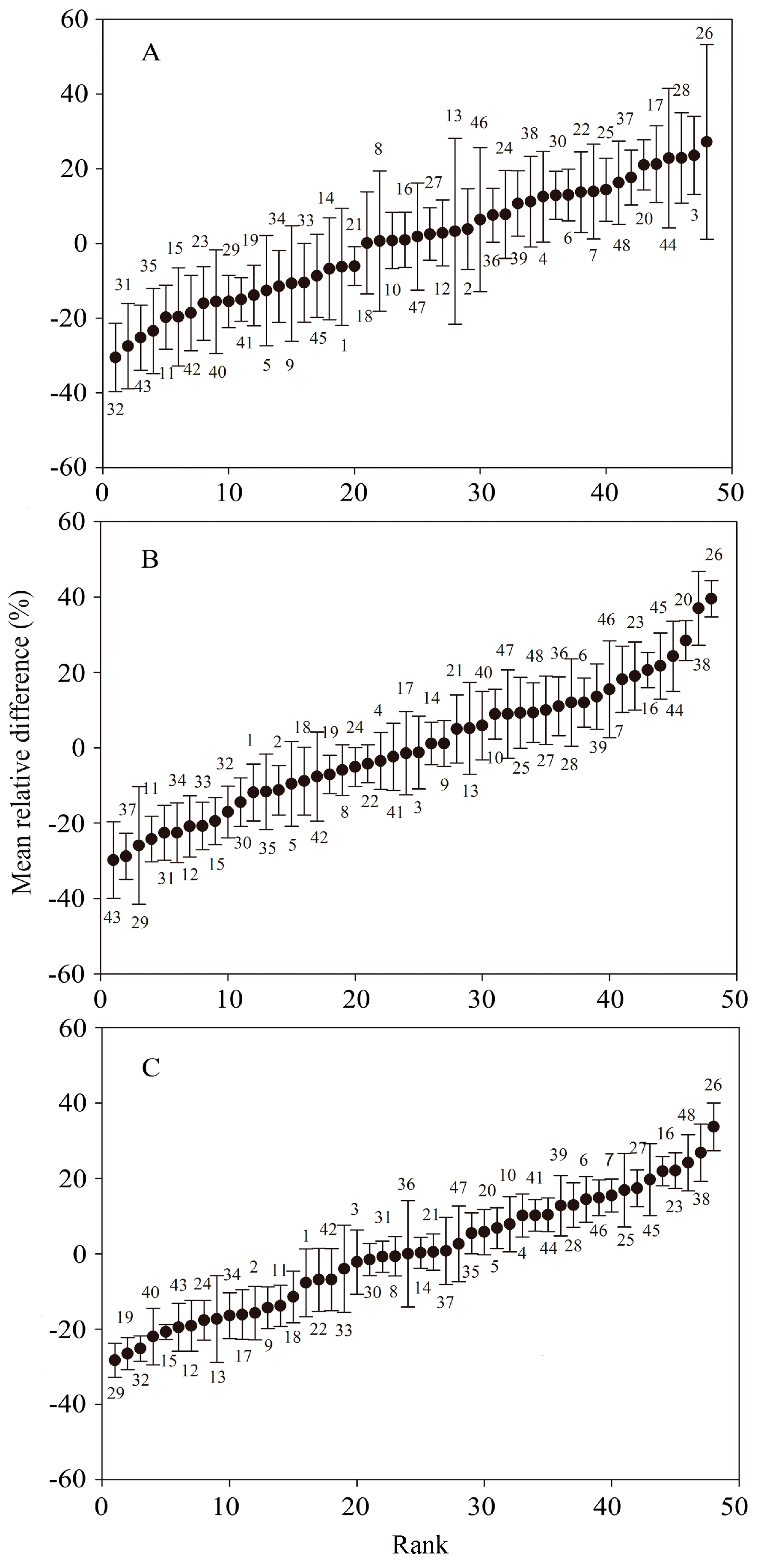
3.3. Temporal Stability of VSM
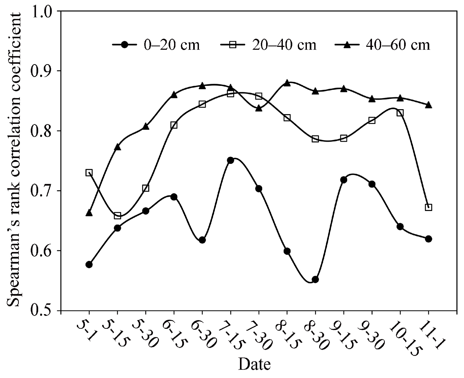
3.3.1. At Slope Scale
3.3.2. At Point Scale
Frequency Distribution
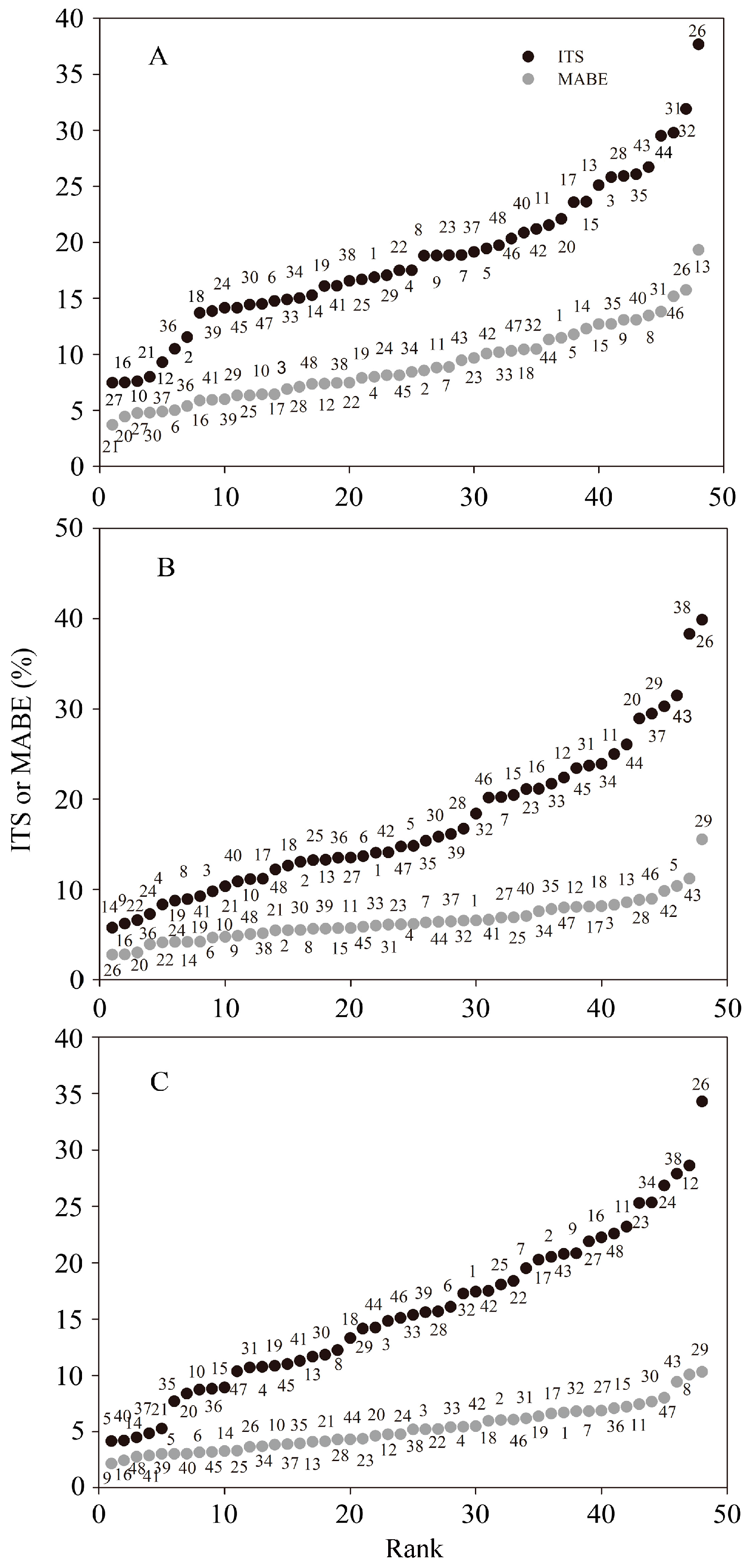
Relative Difference Analysis
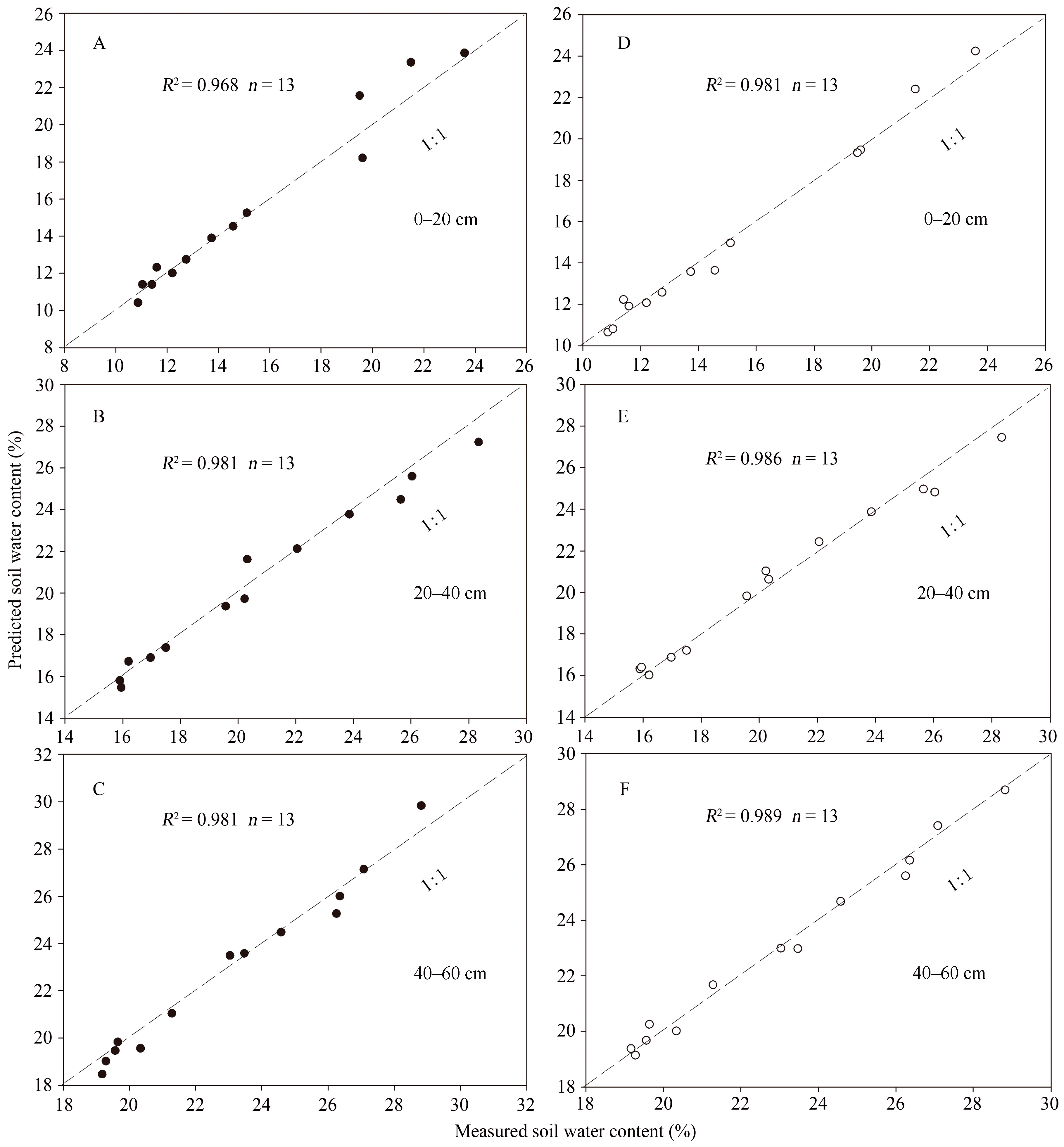
3.4. Identification of Representative Point for Acquisition of Mean VSM
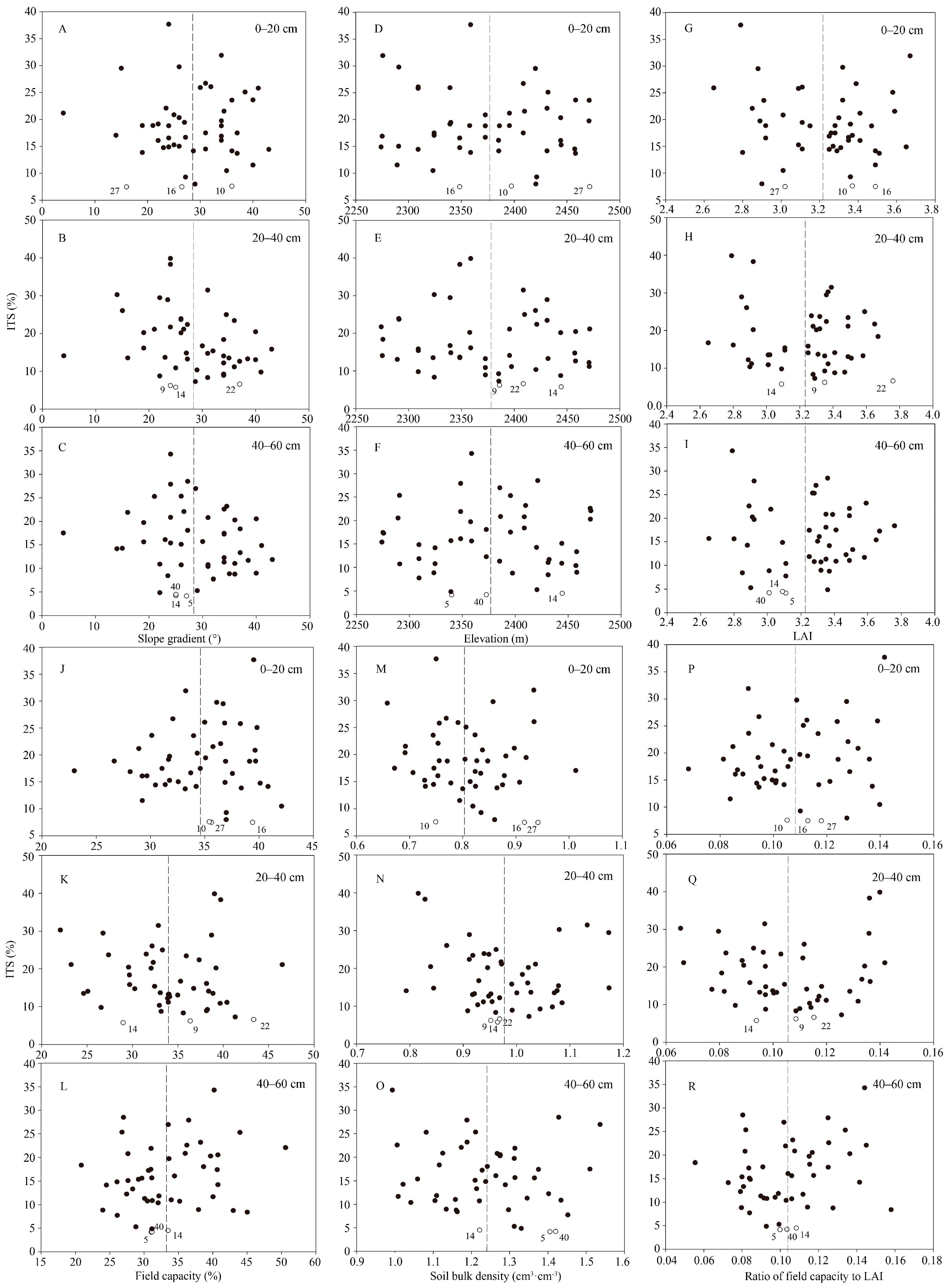
3.5. Factors Affecting the Spatial Pattern of VSM
4. Discussion
4.1. Spatial and Temporal Variability of VSM
4.2. Temporal Stability of VSM
4.3. Representative Points for Mean VSM
4.4. Factors Affecting the Spatial Pattern of VSM
5. Conclusions
Acknowledgments
Author Contributions
Conflicts of Interest
References
- Heathman, G.C.; Larose, M.; Cosh, M.H.; Bindlish, R. Surface and profile soil moisture spatio-temporal analysis during an excessive rainfall period in the Southern Great Plains, USA. Catena 2009, 78, 159–169. [Google Scholar] [CrossRef]
- Penna, D.; Brocca, L.; Borga, M.; Dalla Fontana, G. Soil moisture temporal stability at different depths on two alpine hillslopes during wet and dry periods. J. Hydrol. 2013, 477, 55–71. [Google Scholar] [CrossRef]
- Chaney, N.W.; Roundy, J.K.; Herrera-Estrada, J.E.; Wood, E.F. High-resolution modeling of the spatial heterogeneity of soil moisture: Applications in network design. Water Resour. Res. 2015, 51, 619–638. [Google Scholar] [CrossRef]
- Walker, J.P.; Houser, P.R. A methodology for initializing soil moisture in a global climate model: Assimilation of near-surface soil moisture observations. J. Geophys. Res. Atmos. 2001, 106, 11761–11774. [Google Scholar] [CrossRef]
- Dorigo, W.; de Jeu, R.; Chung, D.; Parinussa, R.; Liu, Y.; Wagner, W.; Fernández-Prieto, D. Evaluating global trends (1988–2010) in harmonized multi-satellite surface soil moisture. Geophys. Res. Lett. 2012, 39, 18405. [Google Scholar] [CrossRef]
- Li, X.; Shao, M.; Jia, X.; Wei, X. Profile distribution of soil–water content and its temporal stability along a 1340-m long transect on the Loess Plateau, China. Catena 2016, 137, 77–86. [Google Scholar] [CrossRef]
- Wang, W.; Zhang, F.; Yuan, L.; Wang, Q.; Zheng, K.; Zhao, C. Environmental factors effect on stem radial variations of Picea crassifolia in Qilian Mountains, Northwestern China. Forests 2016, 7, 210. [Google Scholar] [CrossRef]
- Western, A.W.; Blöschl, G. On the spatial scaling of soil moisture. J. Hydrol. 1999, 217, 203–224. [Google Scholar] [CrossRef]
- Gómez-Plaza, A.; Martı́nez-Mena, M.; Albaladejo, J.; Castillo, V.M. Factors regulating spatial distribution of soil water content in small semiarid catchments. J. Hydrol. 2001, 253, 211–226. [Google Scholar] [CrossRef]
- Jia, Y.; Shao, M. Temporal stability of soil water storage under four types of revegetation on the northern Loess Plateau of China. Agric. Water Manag. 2013, 117, 33–42. [Google Scholar] [CrossRef]
- Duan, L.; Huang, M.; Li, Z.; Zhang, Z.; Zhang, L. Estimation of spatial mean soil water storage using temporal stability at the hillslope scale in black locust (Robinia pseudoacacia) stands. Catena 2017, 156, 51–61. [Google Scholar] [CrossRef]
- Graf, A.; Bogena, H.R.; Drüe, C.; Hardelauf, H.; Pütz, T.; Heinemann, G.; Vereecken, H. Spatiotemporal relations between water budget components and soil water content in a forested tributary catchment. Water Resour. Res. 2014, 50, 4837–4857. [Google Scholar] [CrossRef]
- Perry, M.A.; Niemann, J.D. Generation of soil moisture patterns at the catchment scale by EOF interpolation. Hydrol. Earth Syst. Sci. 2008, 12, 39–53. [Google Scholar] [CrossRef]
- Koch, J.; Cornelissen, T.; Fang, Z.; Bogena, H.; Diekkrüger, B.; Kollet, S.; Stisen, S. Inter-comparison of three distributed hydrological models with respect to seasonal variability of soil moisture patterns at a small forested catchment. J. Hydrol. 2016, 533, 234–249. [Google Scholar] [CrossRef]
- Vanderlinden, K.; Vereecken, H.; Hardelauf, H.; Herbst, M.; Martínez, G.; Cosh, M.H.; Pachepsky, Y.A. Temporal stability of soil water contents: A review of data and analyses. Vadose Zone J. 2012, 11, 280–288. [Google Scholar] [CrossRef]
- Vachaud, G.; Passerat De Silans, A.; Balabanis, P.; Vauclin, M. Temporal stability of spatially measured soil water probability density function. Soil Sci. Soc. Am. J. 1985, 49, 822–828. [Google Scholar] [CrossRef]
- Jacobs, J.M.; Mohanty, B.P.; Hsu, E.C.; Miller, D. SMEX02: Field scale variability, time stability and similarity of soil moisture. Remote Sens. Environ. 2004, 92, 436–446. [Google Scholar] [CrossRef]
- Rötzer, K.; Montzka, C.; Bogena, H.; Wagner, W.; Kerr, Y.H.; Kidd, R.; Vereecken, H. Catchment scale validation of SMOS and ASCAT soil moisture products using hydrological modeling and temporal stability analysis. J. Hydrol. 2014, 519, 934–946. [Google Scholar] [CrossRef]
- Jacobs, J.M.; Hsu, E.C.; Choi, M. Time stability and variability of electronically scanned thinned array radiometer soil moisture during Southern Great Plains hydrology experiments. Hydrol. Process. 2010, 24, 2807–2819. [Google Scholar] [CrossRef]
- Hu, W.; Shao, M.; Reichardt, K. Using a new criterion to identify sites for mean soil water storage evaluation. Soil Sci. Soc. Am. J. 2010, 74, 762–773. [Google Scholar] [CrossRef]
- Zhao, W.; Cui, Z.; Zhang, J.; Jin, J. Temporal stability and variability of soil-water content in a gravel-mulched field in northwestern China. J. Hydrol. 2017, 552, 249–257. [Google Scholar] [CrossRef]
- Cheng, S.; Li, Z.; Xu, G.; Li, P.; Zhang, T.; Cheng, Y. Temporal stability of soil water storage and its influencing factors on a forestland hillslope during the rainy season in China’s Loess Plateau. Environ. Earth Sci. 2017, 76, 539. [Google Scholar] [CrossRef]
- Pan, Y.; Wang, X.; Su, Y.; Li, X.; Gao, Y. Temporal stability of surface soil moisture in artificially revegetated desert area. J. Desert Res. 2009, 29, 81–86, (In Chinese with English Abstract). [Google Scholar]
- Gao, X.; Wu, P.; Zhao, X.; Shi, Y.; Wang, J. Estimating spatial mean soil water contents of sloping jujube orchards using temporal stability. Agric. Water Manag. 2011, 102, 66–73. [Google Scholar] [CrossRef]
- Schneider, K.; Huisman, J.; Breuer, L.; Zhao, Y.; Frede, H. Temporal stability of soil moisture in various semi-arid steppe ecosystems and its application in remote sensing. J. Hydrol. 2008, 359, 16–29. [Google Scholar] [CrossRef]
- Grayson, R.B.; Western, A.W. Towards areal estimation of soil water content from point measurements: Time and space stability of mean response. J. Hydrol. 1998, 207, 68–82. [Google Scholar] [CrossRef]
- Vivoni, E.R.; Gebremichael, M.; Watts, C.J.; Bindlish, R.; Jackson, T.J. Comparison of ground-based and remotely-sensed surface soil moisture estimates over complex terrain during SMEX04. Remote Sens. Environ. 2008, 112, 314–325. [Google Scholar] [CrossRef]
- Mohanty, B.P.; Skaggs, T.H. Spatio-temporal evolution and time-stable characteristics of soil moisture within remote sensing footprints with varying soil, slope, and vegetation. Adv. Water Resour. 2001, 24, 1051–1067. [Google Scholar] [CrossRef]
- Tallon, L.K.; Si, B.C. Representative Soil water benchmarking for environmental monitoring. J. Environ. Inf. 2004, 4, 31–39. [Google Scholar] [CrossRef]
- Duan, X.; Wang, Y.; Xu, L.; Ding, D.; Xiong, W.; Yu, P. Spatial variation of soil electric resistivity of a typical slope in the Xiangshuihe watershed of Liupan Mountains, Northwest China. Acta Pedol. Sin. 2011, 48, 912–921, (In Chinese with English Abstract). [Google Scholar]
- Teuling, A.; Troch, P. Improved understanding of soil moisture variability dynamics. Geophys. Res. Lett. 2005, 32, L05404. [Google Scholar] [CrossRef]
- Lv, L.; Liao, K.; Lai, X.; Zhu, Q.; Zhou, S. Hillslope soil moisture temporal stability under two contrasting land use types during different time periods. Environ. Earth Sci. 2016, 75, 560. [Google Scholar] [CrossRef]
- Liu, Z.; Wang, Y.; Tian, A.; Yu, P.; Xiong, W.; Xu, L.; Wang, Y. Intra-annual variation of stem radius of Larix principis-rupprechtii and its response to environmental factors in Liupan Mountains of Northwest China. Forests 2017, 8, 382. [Google Scholar] [CrossRef]
- Brocca, L.; Melone, F.; Moramarco, T.; Morbidelli, R. Spatial-temporal variability of soil moisture and its estimation across scales. Water Resour. Res. 2010, 46, W02516. [Google Scholar] [CrossRef]
- Brocca, L.; Melone, F.; Moramarco, T.; Morbidelli, R. Soil moisture temporal stability over experimental areas in Central Italy. Geoderma 2009, 148, 364–374. [Google Scholar] [CrossRef]
- Zhao, Y.; Peth, S.; Wang, X.Y.; Lin, H.; Horn, R. Controls of surface soil moisture spatial patterns and their temporal stability in a semi-arid steppe. Hydrol. Process. 2010, 24, 2507–2519. [Google Scholar] [CrossRef]
- Wang, S.; Chen, H.; Fu, Z.; Wang, K. Temporal stability analysis of surface soil water content on two karst hillslopes in southwest China. Environ. Sci. Pollut. Res. 2016, 23, 25267–25279. [Google Scholar] [CrossRef] [PubMed]
- Nielsen, D.R.; Bouma, J. Soil Spatial Variability; Pudoc Publishers: Wageningen, The Netherlands, 1985. [Google Scholar]
- Cosh, M.H.; Jackson, T.J.; Moran, S.; Bindlish, R. Temporal persistence and stability of surface soil moisture in a semi-arid watershed. Remote Sens. Environ. 2008, 112, 304–313. [Google Scholar] [CrossRef]
- Xu, G.; Li, Z.; Li, P.; Zhang, T.; Chang, E.; Wang, F.; Yang, W.; Cheng, Y.; Li, R. The spatial pattern and temporal stability of the soil water content of sloped forestland on the Loess Plateau, China. Soil Sci. Soc. Am. J. 2017, 81, 902–914. [Google Scholar] [CrossRef]
- Jia, X.; Shao, M.; Wei, X.; Wang, Y. Hillslope scale temporal stability of soil water storage in diverse soil layers. J. Hydrol. 2013, 498, 254–264. [Google Scholar] [CrossRef]
- Wang, X.; Pan, Y.; Zhang, Y.; Dou, D.; Hu, R.; Zhang, H. Temporal stability analysis of surface and subsurface soil moisture for a transect in artificial revegetation desert area, China. J. Hydrol. 2013, 507, 100–109. [Google Scholar] [CrossRef]
- Hu, W.; Shao, M.; Han, F.; Reichardt, K. Spatio-temporal variability behavior of land surface soil water content in shrub- and grass-land. Geoderma 2011, 162, 260–272. [Google Scholar] [CrossRef]
- Brocca, L.; Morbidelli, R.; Melone, F.; Moramarco, T. Soil moisture spatial variability in experimental areas of central Italy. J. Hydrol. 2007, 333, 356–373. [Google Scholar] [CrossRef]
- Hawley, M.E.; McCuen, R.H.; Jackson, T.J. Volume accuracy relationships in soil moisture sampling. J. Irrig. Drain. Div. 1982, 108, 1–11. [Google Scholar]
- Robinson, M.; Dean, T.J. Measurement of near surface soil water content using a capacitance probe. Hydrol. Process. 1993, 7, 77–86. [Google Scholar] [CrossRef]
- Vereecken, H.; Kamai, T.; Harter, T.; Kasteel, R.; Hopmans, J.; Vanderborght, J. Explaining soil moisture variability as a function of mean soil moisture: A stochastic unsaturated flow perspective. Geophys. Res. Lett. 2007, 34, 315–324. [Google Scholar] [CrossRef]
- Pan, F.; Peters-Lidard, C.D. On the relationship between mean and variance of soil moisture fields. J. Am. Water Resour. Assoc. 2008, 41, 235–242. [Google Scholar] [CrossRef]
- Owe, M.; Jones, E.B.; Schmugge, T.J. Soil moisture variation patterns observed in Hand County, South Dakota. Water Resour. Res. 1982, 18, 949–954. [Google Scholar] [CrossRef]
- Gao, L.; Shao, M. Temporal stability of soil water storage in diverse soil layers. Catena 2012, 95, 24–32. [Google Scholar] [CrossRef]
- Martínez-Fernández, J.; Ceballos, A. Temporal stability of soil moisture in a large-field experiment in Spain. Soil Sci. Soc. Am. J. 2003, 67, 1647–1656. [Google Scholar] [CrossRef]
- Hupet, F.; Vanclooster, M. Intraseasonal dynamics of soil moisture variability within a small agricultural maize cropped field. J. Hydrol. 2002, 261, 86–101. [Google Scholar] [CrossRef]
- Choi, M.; Jacobs, J.M. Soil moisture variability of root zone profiles within SMEX02 remote sensing footprints. Adv. Water Resour. 2007, 30, 883–896. [Google Scholar] [CrossRef]
- Penna, D.; Borga, M.; Norbiato, D.; Dalla, F.G. Hillslope scale soil moisture variability in a steep alpine terrain. J. Hydrol. 2009, 364, 311–327. [Google Scholar] [CrossRef]
- Kamgar, A.; Hopmans, L.W.; Wallender, W.W.; Wendroth, O. Plot size and sample number for neutron prober measurements in small field trials. Soil Sci. 1993, 156, 213–224. [Google Scholar] [CrossRef]
- Korsunskaya, L.P.; Gummatov, N.G.; Pachepskiy, Y.A. Seasonal changes in root biomass, carbohydrate content, and structure characteristics of gray forest soil. Euransian Soil Sci. 1995, 27, 45–52. [Google Scholar]
- Deng, X.; Wang, Y.; Wang, Y.; Wang, Z.; Xiong, W.; Yu, P.; Zhang, T. Slope variation and scale effect of tree height and DBH of Larix principis-rupprechtii plantations along a slope: A case study of Xiangshui watershed of Liupan Mountains. J. Cent. South Univ. For. Technol. 2016, 36, 121–128, (In Chinese with English Abstract). [Google Scholar]
- Zhang, T.; Wang, Y.; Wang, Y.; Deng, X. Variation of soil bulk density on slopes in the rocky mountains areas of Loess Plateau, Northwest China: A case study of Xiangshuihe small watershed in Liupan Mountains. For. Res. 2016, 29, 545–552, (In Chinese with English Abstract). [Google Scholar]
- Liu, Z.; Wang, Y.; Liu, Y.; Tian, A.; Wang, Y.; Zuo, H.J. Spatiotemporal variation and scale effect of canopy leaf area index of larch plantation on a slope of the semi-humid Liupan Mountains, Ningxia, China. Chin. J. Plant Ecol. 2017, 41, 749–760, (In Chinese with English Abstract). [Google Scholar]
- Zhang, P.; Shao, M. Temporal stability of surface soil moisture in a desert area of northwestern China. J. Hydrol. 2013, 505, 91–101. [Google Scholar] [CrossRef]
- Joshi, C.; Mohanty, B.P.; Jacobs, J.M.; Ines, A.V.M. Spatiotemporal analyses of soil moisture from point to footprint scale in two different hydroclimatic regions. Water Resour. Res. 2011, 47, 99–112. [Google Scholar] [CrossRef]
- Hu, W.; Tallon, L.K.; Si, B.C. Evaluation of time stability indices for soil water storage upscaling. J. Hydrol. 2012, 475, 229–241. [Google Scholar] [CrossRef]
- Guber, A.K.; Gish, T.J.; Pachepsky, Y.A.; van Genuchten, M.T.; Daughtry, C.S.T.; Nicholson, T.J.; Cady, R.E. Temporal stability in soil water content pattern across agricultural fields. Catena 2008, 73, 125–133. [Google Scholar] [CrossRef]
- Biswas, A.; Si, B.C. Identifying scale specific controls of soil water storage in a hummocky landscape using wavelet coherency. Geoderma 2011, 165, 50–59. [Google Scholar] [CrossRef]
- Gómez-Plaza, A.; Alvarez-Rogel, J.; Albaladejo, J.; Castillo, V.M. Spatial patterns and temporal stability of soil moisture across a range of scales in a semi-arid environment. Hydrol. Process. 2000, 14, 1261–1277. [Google Scholar] [CrossRef]
- Cantón, Y.; Solé-Benet, A.; Domingo, F. Temporal and spatial patterns of soil moisture in semiarid badlands of SE Spain. J. Hydrol. 2004, 285, 199–214. [Google Scholar] [CrossRef]
- Jabro, J.D. Estimation of saturated hydraulic conductivity of soils from particle size distribution and bulk density data. Trans. ASAE 1992, 35, 557–560. [Google Scholar] [CrossRef]
- Miller, D.A.; White, R.A. A conterminous United States multilayer soil characteristics dataset for regional climate and hydrology modeling. Earth Interact. 1998, 2, 1–26. [Google Scholar] [CrossRef]
- Jia, Y.; Shao, M.; Jia, X. Spatial pattern of soil moisture and its temporal stability within profiles on a loessial slope in northwestern China. J. Hydrol. 2013, 495, 150–161. [Google Scholar] [CrossRef]
- Qiu, Y.; Fu, B.; Wang, J.; Chen, L. Spatial variability of soil moisture content and its relation to environmental indices in a semi-arid gully catchment of the Loess Plateau, China. J. Arid Environ. 2001, 49, 723–750. [Google Scholar] [CrossRef]
- Teuling, A.J.; Uijlenhoet, R.; Hupet, F.; Van Loon, E.E.; Troch, P.A. Estimating spatial mean root-zone soil moisture from point-scale observations. Hydrol. Earth Syst. Sci. 2006, 10, 755–767. [Google Scholar] [CrossRef]


| Statistic Variables | Soil Depth | Mean | SD | CV |
|---|---|---|---|---|
| Soil bulk density (cm3·cm−3) | 0–20 cm | 0.81 | 0.1 | 9.9 |
| 20–40 cm | 0.98 | 0.1 | 9.3 | |
| 40–60 cm | 1.24 | 0.1 | 11.3 | |
| Field capacity (%) | 0–20 cm | 34.6 | 4.1 | 12.0 |
| 20–40 cm | 34.0 | 5.3 | 15.5 | |
| 40–60 cm | 33.3 | 6.2 | 18.5 | |
| Capillary porosity (%) | 0–20 cm | 38.8 | 5.2 | 13.3 |
| 20–40 cm | 36.9 | 5.0 | 13.5 | |
| 40–60 cm | 36.3 | 5.5 | 15.1 | |
| Non-capillary porosity (%) | 0–20 cm | 24.2 | 5.5 | 22.7 |
| 20–40 cm | 20.3 | 6.5 | 31.9 | |
| 40–60 cm | 12.7 | 5.7 | 44.8 | |
| Total porosity (%) | 0–20 cm | 63.0 | 3.7 | 5.8 |
| 20–40 cm | 57.2 | 4.3 | 7.5 | |
| 40–60 cm | 49.0 | 6.1 | 12.4 | |
| LAI | — | 3.2 | 0.3 | 8.1 |
| Slope gradient (°) | — | 28.5 | 7.9 | 27.7 |
| Elevation (m) | — | 2377 | 58.8 | 2.5 |
| Spatial Variables | Temporal Statistics | 0–20 cm | 20–40 cm | 40–60 cm |
|---|---|---|---|---|
| Mean VSM | Mean (%) | 15.19 | 20.66 | 22.99 |
| Max. (%) | 23.58 | 28.34 | 28.82 | |
| Min. (%) | 10.87 | 15.90 | 19.17 | |
| SDT (%) | 4.37 | 4.23 | 3.35 | |
| CVT (%) | 28.75 | 20.47 | 14.68 | |
| SDS | Mean (%) | 2.98 | 3.89 | 3.89 |
| Max. (%) | 4.55 | 4.64 | 4.38 | |
| Min. (%) | 1.53 | 3.08 | 3.45 | |
| SDT (%) | 1.07 | 0.56 | 0.27 | |
| CVT (%) | 35.95 | 14.41 | 7.03 | |
| CVs | Mean (%) | 19.30 | 19.03 | 17.12 |
| Max. (%) | 22.63 | 20.92 | 18.98 | |
| Min. (%) | 14.11 | 16.31 | 14.63 | |
| SDT (%) | 2.72 | 1.38 | 1.60 | |
| CVT (%) | 14.08 | 7.38 | 9.37 |
| Variables | MRD | ||
|---|---|---|---|
| 0–20 cm | 20–40 cm | 40–60 cm | |
| Elevation | 0.118 | 0.301 * | 0.164 |
| Slope gradient | 0.055 | −0.196 | −0.249 |
| Field capacity | 0.315 * | 0.375 ** | 0.348 * |
| Bulk density | −0.430 ** | −0.357 * | −0.337 * |
| Capillary porosity | 0.327 * | 0.303 * | 0.310 * |
| Non-capillary porosity | −0.082 | −0.209 | −0.488 ** |
| Total porosity | 0.337 * | 0.037 | −0.178 |
| LAI | −0.492 ** | −0.550 ** | −0.463 ** |
© 2018 by the authors. Licensee MDPI, Basel, Switzerland. This article is an open access article distributed under the terms and conditions of the Creative Commons Attribution (CC BY) license (http://creativecommons.org/licenses/by/4.0/).
Share and Cite
Liu, Z.; Wang, Y.; Yu, P.; Tian, A.; Wang, Y.; Xiong, W.; Xu, L. Spatial Pattern and Temporal Stability of Root-Zone Soil Moisture during Growing Season on a Larch Plantation Hillslope in Northwest China. Forests 2018, 9, 68. https://doi.org/10.3390/f9020068
Liu Z, Wang Y, Yu P, Tian A, Wang Y, Xiong W, Xu L. Spatial Pattern and Temporal Stability of Root-Zone Soil Moisture during Growing Season on a Larch Plantation Hillslope in Northwest China. Forests. 2018; 9(2):68. https://doi.org/10.3390/f9020068
Chicago/Turabian StyleLiu, Zebin, Yanhui Wang, Pengtao Yu, Ao Tian, Yarui Wang, Wei Xiong, and Lihong Xu. 2018. "Spatial Pattern and Temporal Stability of Root-Zone Soil Moisture during Growing Season on a Larch Plantation Hillslope in Northwest China" Forests 9, no. 2: 68. https://doi.org/10.3390/f9020068