Drought Impact on Phenology and Green Biomass Production of Alpine Mountain Forest—Case Study of South Tyrol 2001–2012 Inspected with MODIS Time Series

Abstract

Ecological balance and biodiversity of the alpine forest is endangered by global and local climatic extremes. It spurs a need for comprehensive forest monitoring, including in depth analyses of drought impact on the alpine woodland ecosystems. Addressing an arising knowledge gap, we identified and analyzed 2002–2012 aridity related responses within the alpine mountain forest of South Tyrol. The study exploited a S-mode PCA (Principal Component Analysis) based synergy between meteorological conditions rendered by the scPDSI (self-calibrated Palmer Drought Severity Index) and forest status approximated through MODIS (Moderate Resolution Imaging Spectroradiometer) derived NDVI (Normalized Difference Vegetation Index) and NDII7 (Normalized Difference Infrared Index based on MODIS band 7) time series. Besides characterizing predominant forest temporal response to drought, we identified corresponding spatial footprints of drought impact, as well as examined aridity-related changes in forest phenology and biomass production. The latter was further evaluated in relation to forest type, elevation, aspect and slope. Recognized meteorological conditions highlighted: prolonged 2003–2007 mild to extreme drought, and overall regional drying tendencies. Arising remotely sensed forest responses accounted on localized decline in foliage water content and/or photosynthetic activity, but also indicated regions where forest condition improved despite the meteorological stress. Perceived variability in the forest response to drought conditions was governed by geographic location, species structure, elevation and exposition, and featured complexity of the alpine forest ecosystem. Among the inspected biophysical factors elevation had the strongest influence on forest phenology and green biomass production under meteorological stress conditions. Stands growing above 1400 m a.s.l. demonstrated initial increase in annual biomass growth at the beginning of the dry spell in 2003. Conversely, woodlands at lower altitudes comprising considerable share of hardwood species were more prone to biomass decline in 2003, but experienced an overall upturn in biomass production during the following years of the dry spell. Aspect showed moderate effect on drought-related phenology and green biomass production responses. Diverse forest ecosystem responses identified in this study were in line with known local and regional analyses, but also shed some new light on drought induced alternation of forest status.

1. Introduction

The last century, and in particular the past three decades, brought a noticeable change in local and global weather patterns [1,2]. Alternation of temperature, precipitation and insolation that result in prolonged climatic anomaly has recently been highlighted in numerous studies (e.g., [3,4,5,6,7]). Among others, the Alps experience accelerated climate change [8], with two-fold increase of temperature [9] and transformation of precipitation patterns [8,10], which further enhance substantial dryness of the local climate [11]. Despite considerable resistance [12], the alpine environment is affected by climate change, which has triggered uphill shift of vegetation belts [13,14,15], local dieback processes (e.g., [12,14,16]) and overall sway of ecological balance [17,18]. Consequently, alpine forest, which can be deemed as the largest and the most biodiverse land cover of the Alps ([19,20] (p. 13)) is subjected to increasing drought implications.

Drought impact on forest, although seemingly apparent, is still entangled and loaded with uncertainty [21]. Forest drought influence is complex because even though a primary dry spell does not always directly lead to a dieback (e.g., [16,22,23]), it makes trees more vulnerable to secondary damages and disturbances such as windfalls, pest outbreaks [24], fire [25], fungus, parasites and pathogens infestations [14]. Furthermore, trees response to drought is governed by timing and intensity of an event, site-specific environmental conditions [26,27] as well as inter- and intra-species differences [14,28]. This intricacy, still not investigated in depth, is a great hindrance not only for sustainable forest management and silviculture [21], but also for carbon sink efficiency modeling [29,30] and related climate change scenarios [31].

A reliable inspection of drought impact on the alpine forest ecosystem poses major challenges. Traditional dendrochronological surveys are limited to small sites (e.g., [27,32,33,34]) or transects [28] which makes the perception of a drought phenomenon at larger scale very difficult. Moreover, recent studies showed that climate change introduces unsystematic shifts to tree growth patterns [33,35], which presents a new hindrance for forest analyses. Alternative approaches based on flux measurements provide information on forest productivity and drought impact [36] only for small sites with still relatively short time series of observations. Furthermore, flux measurements are aimed at forest stand as a whole and cannot distinguish between forest canopy and understory. In comparison, remote sensing ensures a unique opportunity for reliable acquisition of wall to wall information on environmental conditions at relatively low costs. Abundance of datasets with different spatial and spectral resolution makes remote sensing a versatile and accurate source of forest related information with enhanced temporal resolution [37]. Although optical sensors render only information on the top of the forest canopy, tree foliage was proven to be a good indicator for the assessment of tree condition (e.g., [38,39,40]). Among others, NDVI (Normalized Difference Vegetation Index [41]) and NDII7 (Normalized Difference Infrared Index based on MODIS band 7 [42], aka NBR—Normalized Burn Ratio [43]) gained considerable popularity in the analyses of forest status. While NDVI provides assessment of canopy chlorophyll content, hence photosynthetic activity (‘greenness’), NDII7 approximates foliage spectral properties governed by water content and cell structure. Both indices can be derived using MODIS (Moderate Resolution Imaging Spectroradiometer) datasets that demonstrated overall high potential for forest monitoring (e.g., [39,40,44]), including forest drought analyses [45,46]. Moreover, NDVI time series can be exploited to extract biomass and phenological parameters (e.g., [47,48,49]), shedding more light on vegetation condition.

In this paper we focused on identification and understanding of forest linear response to drought conditions [29,50], and analyzed resultant shifts in forest phenology and green biomass production. The latter topic is still rarely investigated despite its high relevance [51]. The study addressed drought variability of the alpine mountain forest in South Tyrol (2001–2012) and comprised three steps: (i) presentation of regional meteorological drought conditions recognized using scPDSI (self-calibrated Palmer Drought Severity Index; [52]) synthesized over a selection of meteorological stations; (ii) temporal and spatial assessment of drought impact on forest status expressed through changes in canopy photosynthetic activity and water content, approximated, respectively, using MODIS derived 16-day NDVI and NDII7 time series at 250 m spatial resolution; (iii) analysis of drought induced changes in forest phenology and green biomass production as a function of local biophysical conditions. The study employed PCA (Principal Component Analysis; [53]) and concentrated on short- to medium-term drought events of moderate to severe intensity.

2. Materials and Methods

2.1. Study Site

South Tyrol is a typical dry inner Alpine region located in the central part of the Alps. Its topography varies between 190 m a.s.l. (southern Adige Valley) and 3905 m a.s.l. (Mount Ortler), with 86% of the area situated above 1000 m a.s.l. [54]. The local climate is shaped by a Mediterranean-Temperate and Oceanic-Continental gradients following the South-North and West-East directions respectively. Precipitation pattern is strongly regionalized. Annual rainfall sums vary between almost 500 mm in the west (Vinschgau Valley), around 700 mm in the central (Adige Valley and Eisack Valley), and 1200–2000 mm observed in the North-East (Pustertal Valley) part of the region. Moreover, local climate variability is shaped by the temperature gradient [12] and insolation [19], both being a result of altitudinal change.

Woodland occupies around 43% of the area of South Tyrol (namely 3170.5 km²). Forest structure is dominated by coniferous stands (90.1%), with mixed coniferous/deciduous (7.3%), and broadleaved forests (2.6%) near the valley floors. Following climate variability, forest forms altitudinal distribution belts with regional variations governed by local-specific conditions. In the valley floors and on low slopes the most common are hardwood stands of Sessile and Downy Oak (Quercus Petraea and Quercus pubescens, respectively), Hop Hornbeam (Ostrya carpinifolia), Manna Ash (Fraxinus ornus) and Sweet Chestnut (Castanea sativa). With an increase of elevation Downy Oak–Common Beech and Common Beech (Fagus sylvatica) forest is introduced, with Scots Pine (Pinus sylvestris) growing in the most arid locations. Common Beech, Norway Spruce (Picea abies) and Silver Fir (Abies alba) stands are the most abundant on higher elevations, but on sunny and drier slopes are substituted by Scots Pine and European Larch (Larix decidua). The tree line is formed by European Larch and Arolla Pine (Pinus cembra) that gradually transfer into dwarfed trees and shrubs [55].

2.2. Meteorological Conditions

Local 2001–2012 meteorological conditions were approximated by the scPDSI [52] derived for point locations. The index was selected due to its high correspondence with forest status [56,57,58]. Monthly scPDSI values were calculated for 26 meteorological stations evenly distributed within South Tyrol. Coupled site-specific monthly precipitation and temperature observations used for the computation were obtained from the WISKI database of the Hydrographic Office of the Autonomous Province of Bolzano-Südtirol. In order to meet the scPDSI requirements (GreenLeaf Project, [59]) each location was represented by a minimum 25-year-long observation record concluded in December 2012 (For more detailed information on station location and length of used time series please see [60]). Subsequently, all 26 site-specific 2001–2012 scPDSI time series were integrated into a cumulative dataset and introduced into the correlation-matrix based S-mode PCA. Four first resulting PCs, representing herein temporal patterns were assumed to render dominant meteorological variability in South Tyrol between 2001 and 2012 [60].

2.3. MODIS Time Series

The 2001–2013 time series of standard MODIS 16-day MOD13Q1 product (Collection 5) at 250 m resolution was used in the study. For each scene NDVI, band 2 (NIR: 0.840–0.876 µm), band 7 (MIR: 2.105–2.155 µm) and QA (Quality Assessment denoting overall pixel reliability) information were extracted. NDII7 datasets were next computed following the formula:

NDII7 = (NIR − MIR)/(NIR + MIR)

(1)

Application of both indices was motivated by a desire to independently inspect drought impact on forest canopy photosynthesis activity, and foliage water content. All NDVI and NDII7 images were subsequently evaluated against QA. Pixels with the QA-usefulness values below acceptable [61] as well as outliers (confidence level 0.95 according to Chebyshev’s Theorem) were linearly interpolated in the time domain. The process was performed in the TimeStats Software Tool [62] and addressed time-gaps not longer than a single observation. This condition allowed to substitute missing or corrupted observations, but at the same time limited amount of factitious values. As a result, 385 out of 52,394 pixels within the forest mask (Section 2.4) had incomplete 2001–2013 NDII7 time series and were excluded from further analyses. Spatial coverage of NDVI time series was not affected (information on number of forest pixels that underwent interpolation for NDVI and NDII7 time series is presented in Tables S1 and S2, respectively). Data preprocessing of both time series was concluded with the sensor degradation adjustment [63].

2.3.1. Phenology and Green Biomass Production Measures

Yearly, pixel-based phenology and green biomass production measures were derived from the MODIS based complete 2001–2013 16-day NDVI time series using the Phenolo software (for a description see [47]). NDVI data were selected here due to robust seasonality of the signal directly associated with the plant ‘greenness’ [41]. The focus was given to two vegetation productivity metrics: Cyclic Fraction (CF, an approximation of annual seasonal growth), and approximation of Gross Primary Production (GPP, estimated as the integral value of the annual growing season); as well as two season information parameters: Season Length (SL) and Season Begin Day (SBD). All metrics together extensively characterize year-to-year vegetation variability [47,64]. Since the Phenolo algorithm is based on the moving average approach [48], resulting time series comprised parameters only for the 2002–2012 period.

2.4. Ancillary Datasets

Information on forest distribution and forest type within South Tyrol were adopted from the core forest products of the FP7 geoland2 project (EL-04a and EL-04b; [65]). Data gaps present in the dataset and being an effect of cloud cover and topographic shadowing (162 km² in total) were filled in with information from the CORINE Land Cover 2006 dataset [66]. An upscaling from 20 m to 250 m was achieved through spatial averaging, with a threshold of 50% set as a minimum forest cover within each aggregated 250 × 250 m pixel.

A digital elevation model of the whole South Tyrol was provided by the Autonomous Province of Bolzano. In order to adjust the DEM from the original 2.5 m resolution to the MODIS pixel size, a bilinear convolution was applied. Additional layers of slope (in degrees) and aspect (4 expositions) were derived directly from the reprojected DEM using the ArcGIS 10.1 software [67].

2.5. Identification of Drought Impact in Alpine Mountain Forest

Temporal variability of forest status under drought conditions was analyzed using the S-mode PCA. The PCA decomposition investigates inter-relationship within a dataset identifying a dominant temporal variability of its elements. Being a statistical method, physical meaning of PCA results should be evaluated against known or expected variability or process [68]. Following findings from [60], NDVI and NDII7 time series were z-score normalized from a composite mean, and truncated to annual vegetation season time-windows corresponding with a period between April and mid October. Each resulting time series (nNDVI and nNDII7, respectively) was introduced into the covariance-matrix S-mode PCA under the forest mask. The first four PCs obtained for each setup were cross-correlated with the scPDSI temporal patterns, the latter approximating regional meteorological drought conditions. Due to a mismatch in temporal resolution of both datasets (vegetation season vs. complete year, and 16-day vs. month, respectively), correlation was performed for yearly averages. A visual comparison between temporal pattern complemented the statistics [60] and allowed to determine NDVI and NDII7 based PCs with the strongest linear relation to identified meteorological drought conditions, hence representing forest response to drought. Selected PCs were subsequently correlated (pixel based Pearson’s correlation) with their respective vegetation index time-series, resulting in a correlation map (as many maps as PCs selected). These correlation maps can be understood as drought footprints, i.e., the spatial representations of the temporal variability [68]. Each correlation map was classified into three impact classes using the 5th and 95th percentiles of the correlation values distribution. Impact class 1 (0–5th percentile) comprised the most negative, whereas impact class 3 (95–100th percentile) the most positive Pearson’s correlation values. These were interpreted as forest stands responding respectively in contradiction and in agreement with the specific drought temporal variability. Changes in forest phenology and green biomass production within two contrasting response classes were compared for each footprint. Only pixels with a correlation significance level p < 0.1 were considered during analyses.

2.6. Drought Impact Analysis

Further analyses, performed only for forest areas showing the strongest positive and negative linear relations to identified meteorological drought conditions, addressed influence of local biophysical conditions on forest phenology and canopy green biomass production under drought impact. Selected regions were subjected to repeated measures ANOVA (Analysis of Variance) accounting on 4 multi-level environmental factors of:

• forest type (3 levels: coniferous, mixed, broadleaved);
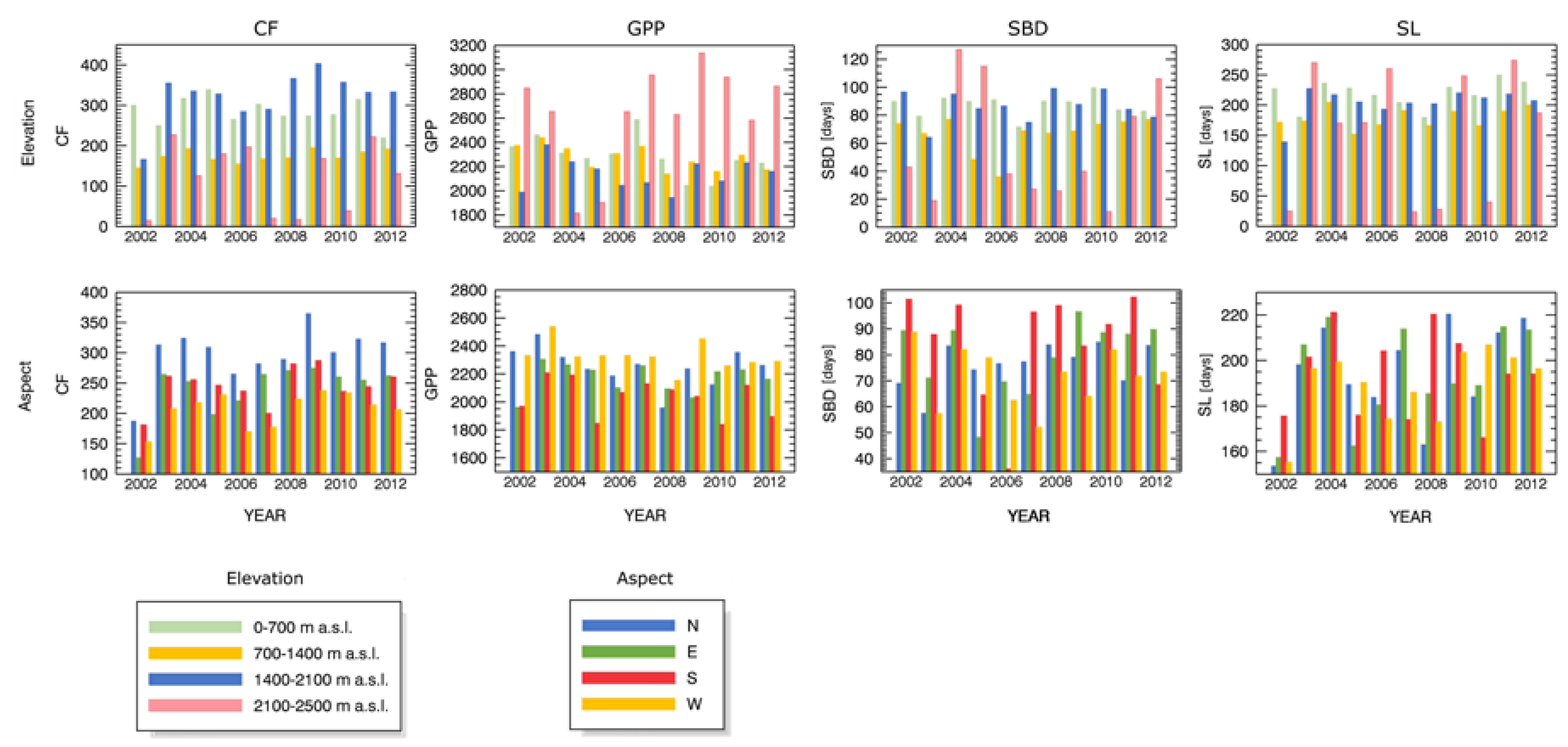
• elevation (4 levels: 0–700 m a.s.l., 700–1400 m a.s.l., 1400–2100 m a.s.l., 2100–2500 m a.s.l.; elevation stratification after [12]);
• exposition (4 levels: N, E, S, W);
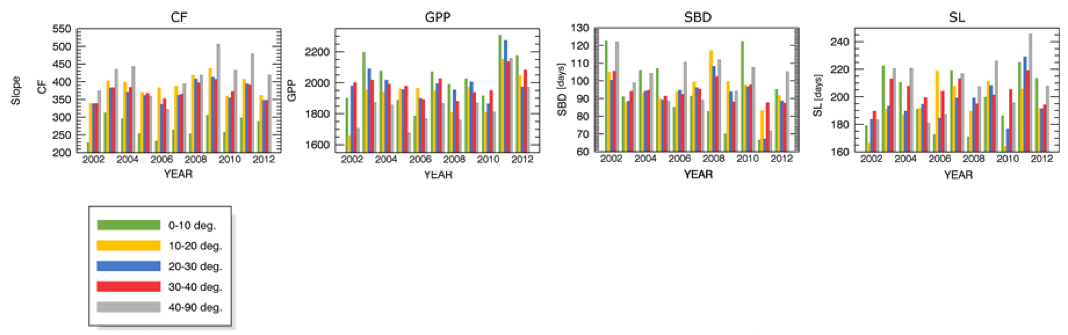
• inclination (5 levels: 0°–10°, 10°–20°, 20°–30°, 30°–40°, 40°–90°).

Repeated measures ANOVA models were run separately for 4 dependent variables of CF, GPP, SL and SBD. The Hujnh-Feldt adjustment was used for all ANOVA runs due to violated sphericity assumption.

3. Results

3.1. Drought Conditions

A synthesis of regional meteorological conditions was determined using the S-mode PCA run on a merged 2001–2012 monthly scPDSI time-series calculated for 26 point locations. As discussed in [60], the first PC (1scPDSI, Figure 1a) accounted for 63% of the data variation and showed a temporal pattern of prolonged drought between 2003 and 2007. The second PC (2scPDSI, Figure 1b) revealed positive anomaly in 2001–2002 as well as isolated short drought conditions at the very beginning and end of the 2001–2012 time series, which explained 9.95% of the data variance. The third and fourth PCs (3scPDSI and 4scPDSI, respectively; Figure 1c,d) showed negative trends, indicating increasing aridity between 2001 and 2012. The 3scPDSI implied an overall drying tendency with enhanced drought conditions in 2009–2011 that explained 7.36% of the data variance. The 4scPDSI depicted scPDSI downturn between 2003 and 2007, which addressed 5.61% of the data variability.

3.2. Forest Temporal Response to Drought Conditions

The PCA run for the nNDVI dataset resulted in the second and third PCs (2nNDVI and 3nNDVI, respectively; Figure 1f,g) showing statistically significant linear relation to the identified drought conditions (

Table 1. Correlation among the scPDSI scores and first four PCs obtained through the covariance-matrix based PCA of the nNDVI (z-score normalized vegetation season NDVI) and nNDII7 (z-score normalized vegetation season NDII7) time series. Linear correspondence was calculated for yearly averaged time series.

	nNDVI				nNDII7
	1nNDVI	2nNDVI	3nNDVI	4nNDVI	1nNDII7	2nNDII7	3nNDII7	4nNDII7
1scPDSI	−0.573	0.713 *	−0.310 *	−0.374	−0.717 *	−0.374	−0.189	−0.608 *
2scPDSI	−0.321	0.608 *	−0.360 *	−0.349	−0.199 *	−0.278	−0.260	−0.502 *
3scPDSI	−0.155	−0.337 **	−0.632 *	−0.160	−0.559 *	−0.257	−0.131	−0.023 *
4scPDSI	−0.489	−0.013 **	−0.257 *	−0.261	−0.010 *	−0.243	−0.288	−0.583 *

* Significant at the level p < 0.05.

, p < 0.05). The 2nd PC, despite a sound correlation with the 1scPDSI and 2scPDSI, revealed strong variation of the score that impeached its physical meaning. The 3nNDVI revealed an abrupt upturn of photosynthetic activity of forest ecosystem in 2003. This anomaly was followed by a gradual decrease of the score, well corresponding to the enhanced drought intensity and increasing aridity trend. Complementary visual evaluation suggested the 3rd PC to render a physically meaningful changes in forest canopy photosynthetic activity related to drought conditions.

Analysis based on the nNDII7 time series revealed in the first and fourth PCs (1nNDII7 and 4nNDII7, respectively; Figure 1i,l) forest response being significantly correlated with the 2003–2007 drought (Table 1, p < 0.05). Both principal components depicted increase in canopy water content after 2008, which is congruent with a retreat of drought conditions. Progressing aridity in the region was indicated by a significant correlation between the 4nNDII7 and 4scPDSI (Table 1). Since the 1nNDII7 did not render a decrease in vegetation vigor related to the drought inception in 2003, the 4nNDII7 was recognized to have a stronger physical meaning of drought impact on canopy water content within forest ecosystem.

3.3. Forest Spatial Response to Meteorological Drought Conditions

The prolonged 2003–2007 meteorological drought conditions were best reflected in the 4nNDII7 PC. Featured diminished water content of forest canopy between 2004 and 2007 was observed mainly in the west and central part of South Tyrol (Figure 2a, class 3; correlation values range 0.218 to 0.514) and related mostly to coniferous stands growing between 700 and 2100 m a.s.l. (

Table 2. Drought footprints of the 4nNDII7 and 3nNDVI PCs (Figure 2a,b, respectively), inspected within four multilevel environmental factors of forest type, elevation, exposition and aspect. Class 3 denotes regions with the strongest positive, whereas class 1 the strongest negative fit to the respective PCs depicted in Figure 1g,l.

	4nNDII7		3nNDVI
	Drought Impact		Drought Impact
[%]	Class 1	Class 3	Class 1	Class 3
Coniferous	91.04	95.38	76.10	96.85
Broadleaved	1.88 *	0.58 *	3.65 *	0.33 *
Mixed	7.08 *	4.05 *	20.25	2.82 *
0–700 m a.s.l.	1.88 *	3.90 *	13.11	0.50 *
700–1400 m a.s.l.	33.38	54.77	63.24	31.29
1400–2100 m a.s.l.	64.74	33.96	20.66	68.13
2100–2500m a.s.l.	-	7.37	2.99 *	0.50 *
N	25.29	27.17	4.65	62.07
E	17.63	18.79	30.71	11.78
S	27.75	34.54	49.21	5.15
W	29.34	19.51	15.44	21.00
0–10 deg.	18.50	3.76	14.27	3.90
10–20 deg.	34.54	20.38	36.43	20.08
20–30 deg.	36.56	51.01	40.91	56.85
30–40 deg	10.26	23.70	7.97	18.67
40–90 deg.	0.14 *	1.16 *	0.41 *	0.50 *

* Category with less than 50 observations.

). This drought impact was frequently preset at slopes with south exposition and moderate inclination. The opposite response indicating NDII7 increase between 2004 and 2007 (Figure 2a, class 1, correlation values range −0.445 to −0.203) occurred especially on the lower slopes of the Eisack Valley (central region) and in the east-most part of South Tyrol (Pustertal). It was more common on west and south facing slopes of mid to high altitudes and low to moderate inclination (Table 2).

The gradual decrease of forest ‘greenness’ captured by the 3nNDVI and associated with increasing aridity of local climate, was mostly seen in coniferous forest (Table 2) on north exposed sites in the central-north and west parts of South Tyrol (Figure 2, class 3, correlation values range 0.284 to 0.600). Indicated stands were the most common at medium to high altitudes with a clear preference for 1400–2100 m a.s.l. elevation and moderate slopes (Table 2). The reverse response revealing a NDVI drop in 2003 followed by a gradual increase of forest photosynthetic activity (Figure 2, class 1, correlation values range −0.632 to −0.316) was the most frequent in the Eisack Valley. It was observed mainly for coniferous stands and mixed forest (Table 2) at south and east exposed slopes. Medium elevation range (700–1600 m a.s.l.) and moderate inclination (20–30 deg.) were the most common among regions associated with this response.

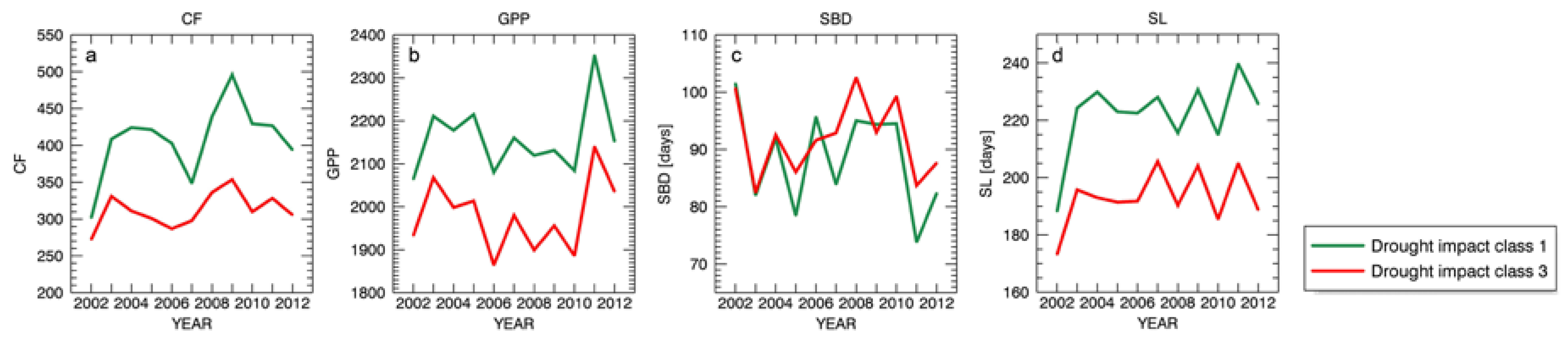
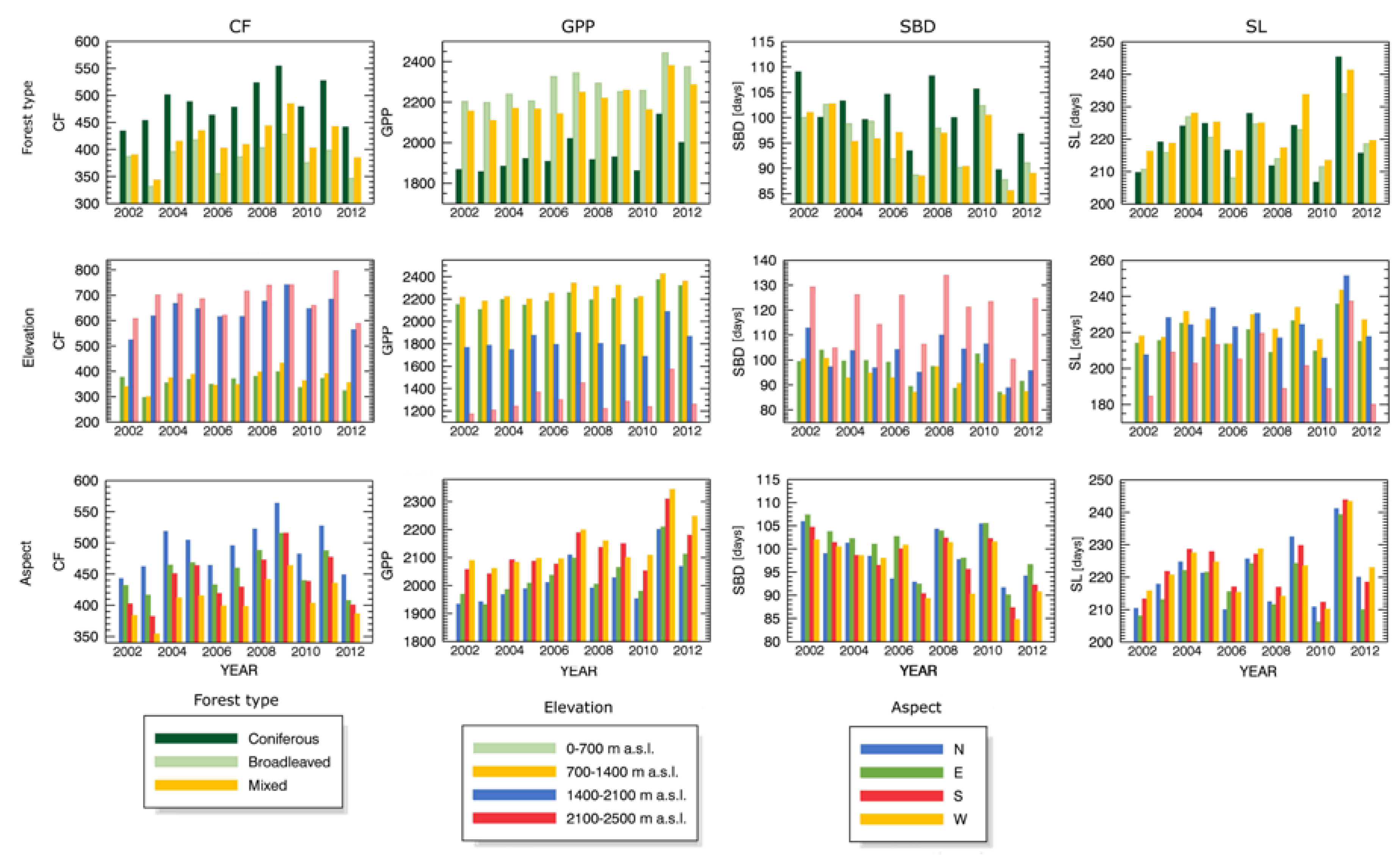
3.4. Drought Impact on Phenology and Green Biomass Production

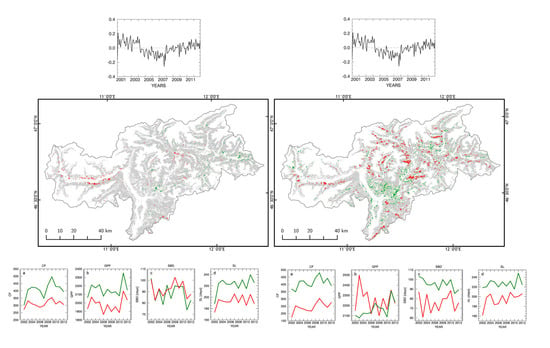
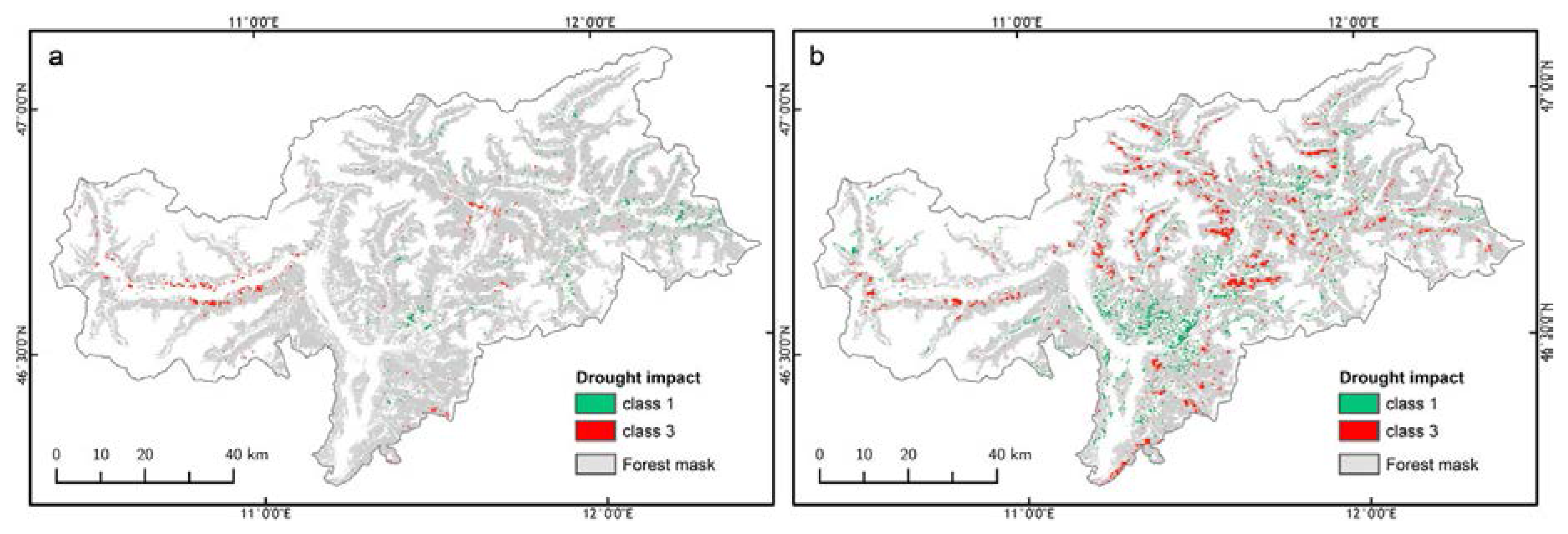
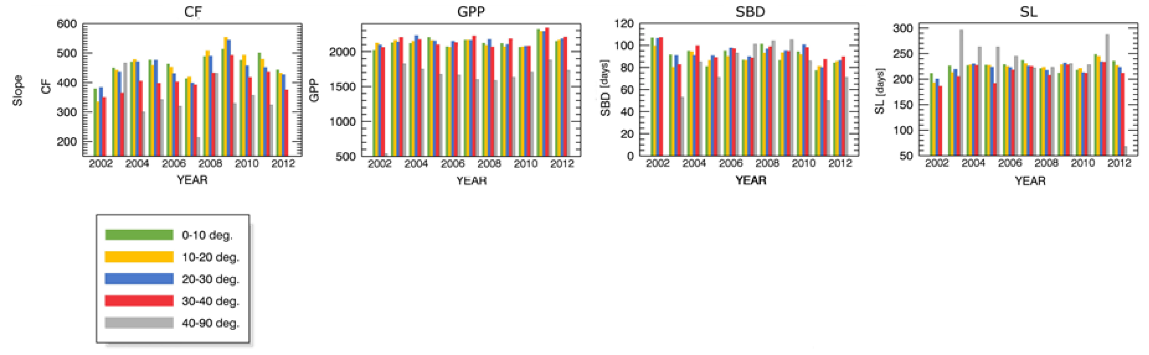
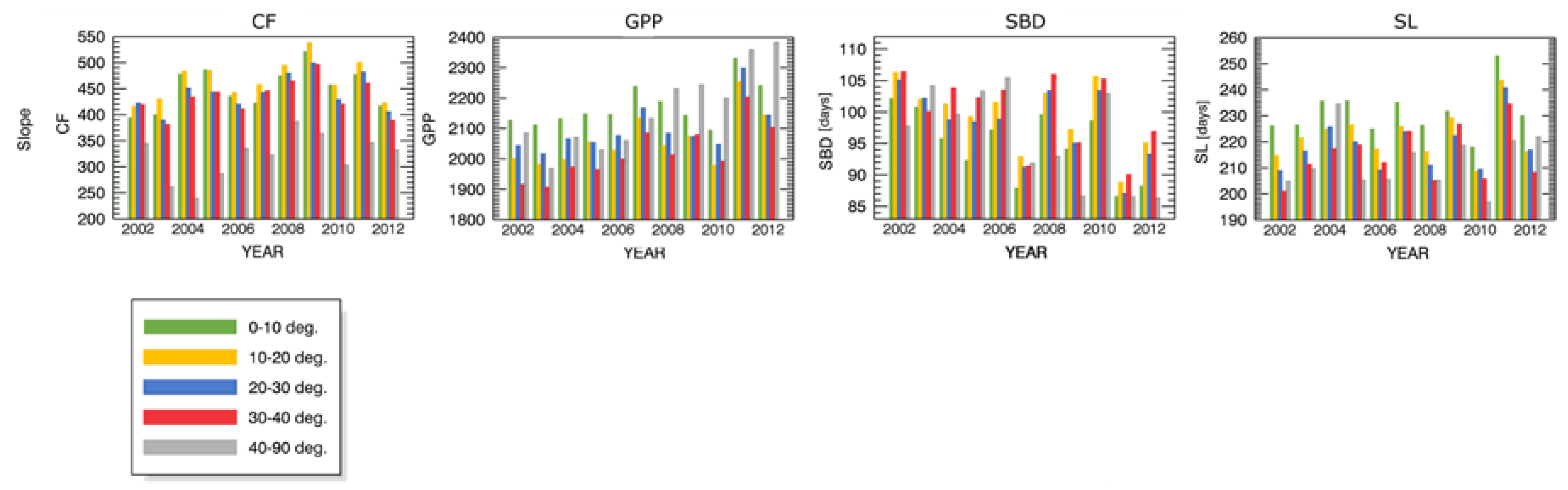
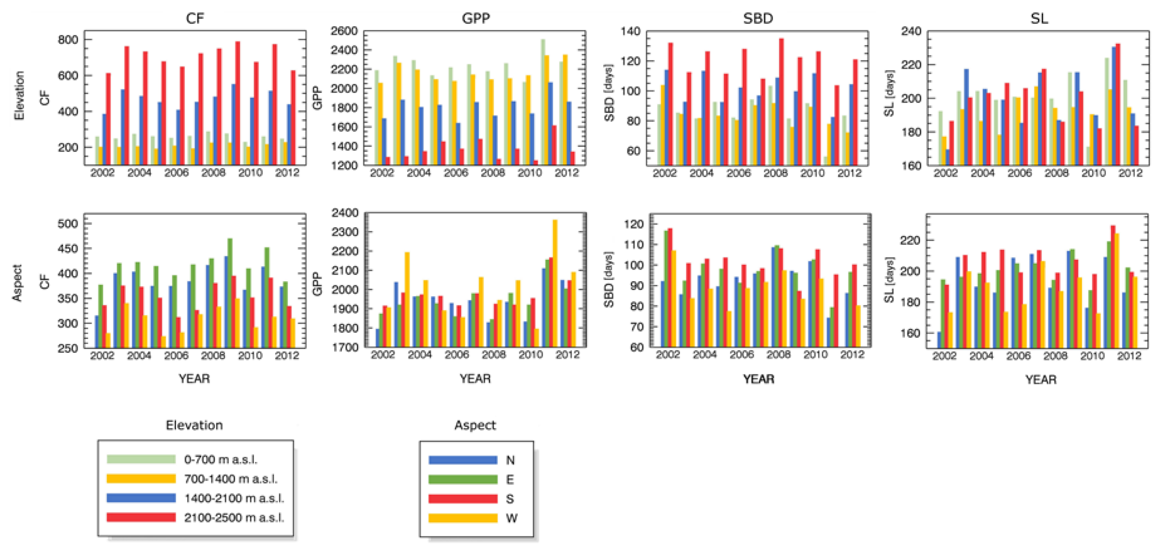
3.4.1. Changes in Forest Canopy Water Content—4nNDII7 PC

Diverse regional development of forest canopy water content between 2002 and 2012 was related to significant differences in forest phenology and green biomass production (

Table A1. Overall significance of differences in 2002–2012 phenology and green biomass production observed within the spatial representation of the 4nNDII7 PC, considered without and with stratification into drought impact classes (3 levels).

	Time			Time * Impact Class			Error
	df	F	p	df	F	p	df
CF	8.744	503.359	0.000	17.489	25.996	0.000	121,146.020
GPP	9.200	167.685	0.000	18.401	3.728	0.000	125,600.330
SBD	9.024	138.845	0.000	18.047	4.729	0.000	125,012.369
SL	9.351	125.195	0.000	18.702	3.434	0.000	129,545.465

Abbreviations: CF—cycling fraction; GPP—Gross Primary Production; SBD—Season Begin Day; SL—Season Length.

, Figure 3). Stands revealing the lowest NDII7 between 2004 and 2007 (impact class 3) showed depleted CF (Figure 3a) accompanied by an overall 2003–2010 GPP decrease (Figure 3b), both being observed after a clear productivity increases in 2003. Although 2003 marked an earlier SBD (Figure 3c), the consecutive years showed progressive delay in the vegetation onset. At the same time length of the growing season demonstrated a strong inter-annual variation without a clear trend (Figure 3d).

A subsequent inspection of forest phenology and green biomass production in relation to site-specific environmental conditions showed considerable variation (Figure 4). Elevation had the strongest impact on all four inspected indices. Drought ingress in 2003 spurred CF rise within stands located above 1400 m a.s.l., but had almost no influence on forest growing at lower altitudes. Simultaneously, although GPP increase in 2003 was observed up to 2100 m a.s.l., GPP 2003–2007 increasing tendency was depicted exclusively at the highest elevations, and was paired with SL prolongation. Stands located below 1400 m a.s.l. demonstrated the earliest vegetation onset and a distinct 2002–2006 shift towards earlier SBD (pairwise comparison p < 0.05).

Aspect revealed limited impact on forest phenology and green biomass production within stands showing diminished foliage water content between 2004 and 2007 (Figure 4). North- and west-exposed woodlands demonstrated the greatest CF and GPP increase in 2003 and 2011. At the same time, the most significant CF decrease aligned with drought conditions was observed for west and south facing locations. Drought conditions enhanced aspect-specific differences in SL and SBD temporal responses. Vegetation onset occurred earlier in 2003, with the biggest change observed for west, south and east facing stands. On the contrary, 2011 marked particularly early SBD at all sites but south. Those anomalies were partly consistent with extended SL. A clear season length prolongation tendency was noted for east oriented areas only until 2007.

A comparison among forest types was not performed due to insufficient representation of broadleaved and mixed woodland (Table 2). Role of inclination in governing forest status under drought conditions was limited and is briefly discussed in Appendix A.1.

Forest rendering elevated canopy water content, associated with the 4nNDII7 drought impact class 1, revealed higher green biomass production as well as on average 28.9 days longer vegetation season (Figure 3b,d, respectively) comparing with the region depicted by class 3 response. CF showed here an overall increasing tendency with two strong upturns in 2003 and 2008–2009 (Figure 3a). A GPP increment spurred in 2003 lasted only until 2005 (Figure 3b). No clear change trend was identified for SBD, which was characterized by intense year-to-year variability with the most abrupt shift towards the earlier vegetation onset in 2003 and 2011 (Figure 3c). Season length became greatly prolonged in 2003 and despite inter-annual variability, remained extended throughout the whole time of the analysis (Figure 3d).

Further analyses revealed influence of biophysical factors on forest phenology and green biomass productivity within the 4nNDII7 class 1 areas (Figure 5). Stands growing above 1400 m a.s.l. showed here not only the highest overall seasonal production, but also the strongest CF and GPP gains in 2003. The latter were coupled with sooner vegetation onset and longer SL. A gradual 2003–2010 GPP decrease was observed above 1400 m a.s.l. and contrasted with response of stands located at lower altitudes. Disparity in vegetation onset was the biggest for 2004 and 2006–2010.

Aspect marked limited influence on changes in forest status (Figure 5), where all expositions fostered similar temporal responses. Although east-facing sites as the only one did not reveal substantial CF and GPP increase in 2003, they reported steady 2002–2009 GPP rise and statistically significant shift towards earlier SBD (pairwise comparison, p < 0.02). Despite the biggest SBD advancement in 2003 was observed for north exposition, the greatest 2003 SL prolongation occurred on south-facing slopes. The greatest differences in SBD and SL among aspects were noted for 2003–2005 and in 2010.

Restricted representation of broadleaved and mixed forest stands (Table 2) inhibited forest type specific analyses. Slope demonstrated limited influence on forest phenology and green biomass production. Relevant results are presented in Appendix A.1.

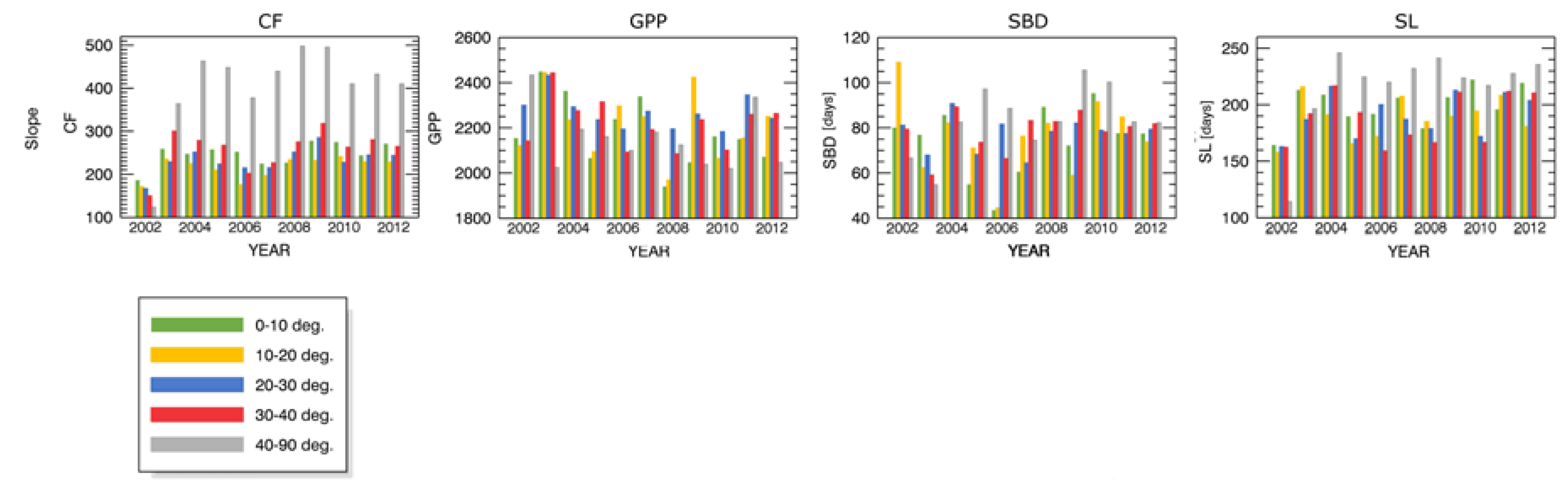
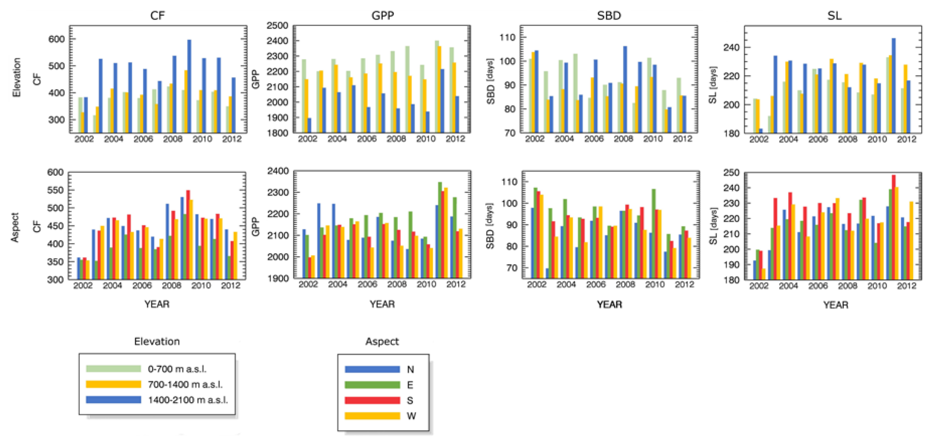
3.4.2. Changes in Forest Canopy Photosynthetic Activity—3nNDVI PC

Identified through the 3nNDVI PC divergent trends in photosynthetic activity of forest canopy were complementary to significant differences in forest phenology and green biomass production (

Table A3. Overall significance of differences in 2002–2012 phenology and green biomass production observed within the spatial representation of the 3nNDVI PC, considered without and with stratification into drought impact classes (3 levels). Abbreviations correspond with Table A1.

	Time			Time * Impact Class			Error
	df	F	p	df	F	p	df
CF	8.892	724.295	0.000	17.784	63.582	0.000	214,367.891
GPP	9.279	241.944	0.000	18.558	48.716	0.000	223,701.831
SBD	9.021	189.351	0.000	18.042	22.824	0.000	217,481.749
SL	9.366	173.060	0.000	18.732	20.009	0.000	225,791.834

, Figure 6). Stands experiencing the decline in forest ‘greenness’ (class 3) were characterized by low, but overall increasing CF with two intense gains in 2003 and 2009 (Figure 6a). Coupled GPP development (Figure 6b) accounted on a massive upturn in 2003, followed by an equally strong drop, and a subsequent intense variability in biomass levels between 2006 and 2012. SBD varied greatly over the whole observation period, and showed no clear change tendency (Figure 6c). Simultaneously, gradual SL prolongation was observed (Figure 6d). Drought ingress in 2003 was aligned with sooner SBD and longer growing season.

Influence of biophysical factors on forest phenology and green biomass production within the 3nNDVI class 3 drought response was moderate. Stands placed at 1400–2100 m a.s.l. showed higher CF with greater inter-annual variability (Figure 7). In contrast, elevation-dependent differences in GPP were less distinct (but statistically significant, pairwise comparison, p < 0.005). Drought ingress in 2003 clearly spurred CF and GPP at higher elevations. Vegetation onset within forest growing below 1400 m a.s.l. occurred significantly sooner than SBD at higher altitudes (pairwise comparison, p < 0.001), which contrasted with longer SL observed at higher elevations.

Relation between exposition and forest status within regions subjected to NDVI decrease was complex (Figure 7). North slopes showed the greatest CF increase in 2003 and the highest overall seasonal production, but revealed a clear GPP decline after 2003. West-exposed stands had, in general, the highest GPP coupled with the lowest CF, as well as the smallest productivity gains associated with the ingress of drought conditions in 2003. Differences in vegetation onset analyzed among aspect classes showed strong inter-annual variability with no clear mutual relations. Season length also varied greatly among expositions, and its relation to SBD was not clear.

Inclination was found to have limited impact on shaping forest response to drought conditions, and relevant results are presented in Appendix B.1. Analysis of drought response being a function of forest type was not performed due to the insufficient number of pixels associated with broadleaved and mixed stands (Table 2).

Forest stands associated with the 3nNDVI class 1, and fostering an initial drop of canopy ‘greenness’ in 2003 followed by a long-term increase in photosynthetic activity showed high CF with an overal upturn tendency (Figure 6a). This response was paired with gradually increasing GPP (Figure 6b). Remarkably, both biomass production measures declined in 2003. Vegetation onset occurred here on average 19.6 days later comparing with regions recognized through the 3nNDVI class 3 response, and revealed a clear shift towards earlier SBD (Figure 6c). In contrast, SL showed no long-term trends and was roughly 32.6 days longer than observed within the impact class 3 (Figure 6d).

Forest phenology and green biomass production associated with the overall NDVI increase was further shaped by local environmental conditions. Coniferous forest reported here clearly higher CF with lower annual biomass integral (Figure 8). Ingress of drought conditions in 2003 resulted in CF and GPP declines, as well as delayed season begin day observed for mixed stands. On the contrary, needle leaved woodland reported in 2003 sooner vegetation onset. No meaningful differences were reported for SL.

Stands growing below 1400 m a.s.l. revealed lower CF of suppressed temporal variability with productivity decline in 2003. Forests at higher elevations were characterized by lower GPP, but marked CF rise aligned with the drought ingress. SBD showed a minor and nonlinear relation to altitude. Earlier vegetation onset was observed in 2003 only between 1400 and 2100 m a.s.l. SL revealed limited disparity between elevation classes, with the most apparent differences noted before 2006.

Aspect factor governed linear diversification between forest phenology and green biomass production, where all expositions followed alike, index-dependent temporal variability (Figure 8). The highest CF was observed at north-facing slopes, where also an increase in green biomass production was reported in 2003. GPP showed a clear disparity between south-west and north-east exposed sites, with the former having higher productivity yield. Small exposition-specific differences in SBD were observed only before 2007. Diversification among aspects was also very limited for SL.

Role of inclination on forest phenology and green biomass production within areas rendering NDVI incline is synthesized in Appendix B.1.

4. Discussion

4.1. Meteorological Drought Conditions and Forest Temporal Response

The 2001–2012 meteorological drought conditions in South Tyrol were characterized by two temporal patterns: (i) 2003–2007 mild to extreme persistent drought event depicted in the 1scPDSI PC; and (ii) gradual scPDSI decline captured in the 3scPDSI and 4scPDSI scores. Both were in strong accordance with local events as well as Pan-European meteorological conditions [60,69].

Principal components representing dominant temporal variability of forest canopy were evaluated against recognized meteorological conditions, which proved them to have relevant physical meaning. Although identified drought conditions did not dominate forest response, its linear interrelationship with vegetation status was certain. The anticipated impact of the 2003–2007 drought conditions was visible in the 2004–2007 diminished canopy water contend depicted in the 4nNDII7 PC. The observed lag between drought inception in 2003 and decrease of canopy water content could be explained by forest resistance governed by local environmental conditions [28,70], trees species characteristics and adaptation strategies [71,72], as well as local tree competition [14,22,27,34].

The regional drying tendency was rendered in the downturn of photosynthesis activity captured in the 3nNDVI PC (class 3). This subtle trend is supported by the long-term climate transformation suggested by [8]. Moreover, the perceived decline is further enhanced by the abrupt NDVI increase in 2003. This gain can be explained by enhanced productivity triggered by the 2003 Pan-European heatwave [73]. The reversed interpretation of the 3nNDVI PC (class 1) indicated the gradual ‘greenness’ upturn initiated with the massive NDVI decline, which can be explained as drought triggered wilting, or even dieback followed by a subsequent re-growth of better adjusted vegetation [14]. Such phenomenon has been already observed in South Tyrol [16]. Interestingly, some forest stands reported also NDII7 increase, which could be supported by findings of [74].

The presented approach based on statistical PCA decomposition does not distinguish between the cause of changes in the remotely-sensed time series, therefore treats alike stress and disturbance related signal. To our knowledge, South Tyrol has not been affected between 2001 and 2013 by any major forest disturbance event, such as forest fires or wind throws, that might impact PCA results. Local events are rather unlike to affect the leading variability and are depicted in the PCs of the higher order, which have not been discussed here.

4.2. Alpine Forest Response to Identified Meteorological Drought Conditions

4.2.1. Changes in Foliage Water Content 2004–2007 (4nNDII7 PC)

Diminished foliage water content between 2004 and 2007 was the most apparent in the mountain and subalpine forests composed of Norway Spruce, Silver Fir and Downy Oak with regional inclusions of Scots Pine and European Larch trees. Those stands were often located on poor mountain soils developed on silicate rocks [55]. The contrasting response depicting increased canopy water content and enclosed in the 4nNDII7 class 1 indicated Norway Spruce stands with additional share of Downy Oak and Common Beech trees that frequently grew on silt and carbonate soils [55]. Higher share of broadleaved trees, as well as better soils could explain increase in foliage water content, and higher forest productivity observed within the 4nNDII7 drought impact class 1. Detailed analyses supported by additional data are however essential to fully comprehend those results.

The drought ingress in 2003 affected alike phenology and production within both inspected 4nNDII7 impact classes. Short-lived GPP and CF increases observed in 2003 are in line with [27] and could be explained not only by the earlier SBD and longer SL, but also intensified vegetation growth at higher altitudes, which is normally constrained by the temperature gradient [73,75]. Extended dryness led however to divergence in CF values within both impact classes, which can be related to site-specific differences and environmental conditions such as soil structure, and forest species distribution [28,33,76,74]. Although areas showing depleted NDII7 (class 3) were mostly detected in the Vinschgau Valley, which is the driest region of South Tyrol, expected higher drought adjustment of trees shown by [77] was not observed. Conversely, 2003–2010 GPP downturn depicts a decline in status of the coniferous mountain forest. It is feasible that longer or more intense drought event(s) could exceed adaptation and mitigation abilities of some forest communities and lead to local diebacks [12,78].

Interestingly, longer SL after 2003 was coupled for class 3 with delayed SBD between 2004 and 2008. This could potentially be governed by a relation between Norway Spruce growth and summer temperature conditions during the previous vegetation season [33]. However, an exact link between drought conditions and phenology has still to be made [79]. Considerably longer vegetation season noted for class 1 potentially results from different climatic conditions between the western and central-eastern parts of South Tyrol, and further affects aforementioned productivity differences between two considered impact areas.

4.2.2. Changes in Foliage Photosynthetic Activity (3nNDVI)

Declining forest ‘greenness’ was the most common within Norway Spruce mountain forest [55] growing in majority at north-exposed slopes (Table 2). Although Norway Spruce has moderate drought tolerance, which is especially clear at lower altitudes [80], high elevation and shaded locations could partly mitigate impact of the arising drought stress [27]. Moreover, beneficial effect of released temperature gradient constrain, led to productivity increase in 2003 [73]. The following years showed however CF and GPP decline, which is in line with findings of [81] who indicated that forest drought response at mesic sites can be stronger than at xeric locations. Furthermore, due to shallow root system as well as poor soils and rocky bedrock present at high elevations, Norway Spruce is susceptible to elevated temperature and depleted soil moisture [33]. Despite GPP decline, the overall CF upturn was observed. This decoupled response could be partly explained by longer SL, and accelerated biomass production of hardwood vegetation present within the area.

Increase in canopy photosynthetic activity rendered in the 3nNDVI class 1, was observed within stands dominated by Downy Oak, Sessile Oak, Hop Hornbeam, Sweet Chestnut, Manna Ask and Common Beach trees, with Scots Pine in dry and hot locations, as well as Norway Spruce on higher and shaded spots [55]. Most of these stands grows at lower altitudes that are more prone to temperature increase and rain shortfall [82]. Furthermore woodland in question is often located on endemic, poor silicate soils, which cannot mitigate arid conditions. Consequently, the observed overall productivity increase and earlier vegetation onset tendency suggest an upturn in hardwood trees status resulting from better adjustment to drought conditions [14,76]. Local observations and documented Scots Pine dieback in the Eisack Valley [16] demonstrated drought triggered change in competition between coniferous and broadleaved trees, where hardwood understory species such as Downy Oak and Hop Hornbeam replaced evergreen trees withered after the 2003 heat-wave. Alike transitions were observed in other alpine valleys (e.g., [14,22,70]) and are often attributed on climate change [83,84]. The observed tendency towards the earlier vegetation onset is in line with other studies [12,85,86].

4.3. Drought Impact under Different Biophysical Conditions

Forest phenology and green biomass production is related to site-specific environmental characteristics. This relation was further shaped by drought conditions. Elevation had the most important influence on diversification of forest growth during the discussed meteorological stress. The impact of altitude varied between locations and drought impact classes. Although [87] demonstrated Pan-European forest productivity decline in 2003, our study revealed GPP and CF drop only for stands growing below 1400 m a.s.l. within the 3nNDVI class 1 response. Forest at higher elevations showed GPP and CF increases in 2003, which for some location was noted also in 2004. Furthermore, the 3nNDVI class 3 indicated the productivity gain already at 700 m a.s.l. Abovementioned discrepancy from [87] could arise from higher spatial resolution of data used in our study. Moreover, our findings agree with demonstrated by [80] diverse effect of altitude on different tree species under heat wave conditions, as well as productivity increase observed at higher elevations due to drought-released temperature gradient [73,75,82]. The shift towards earlier SBD showed for some stands growing below 1400 m a.s.l. (3nNDVI class 1 and 4nNDII7 class 3), possibly reflects climate alternation towards warmer and dryer conditions [84], which is particularly vivid at lower altitudes [82]. Finally, the counterintuitive relation between elevation and CF could be explained by larch trees, as well as canopy openings, both being more frequent towards the upper tree line. Remarkably, the upturn in seasonal productivity was not coupled with prolongation of vegetation season.

Drought impact on forest green biomass production and phenology showed moderate diversification in relation to exposition. In most of the cases, all aspect classes followed alike, index-specific temporal variability and revealed only minor drought-induced differences. Disparities in forest status among aspects originate presumably from species distribution and exposition governed water scarcity [27,28], which explains enhanced inter-exposition variation under drought stress conditions. Since [88] showed SBD to be controlled by temperature rather than precipitation, as well as highlighted influence of photoperiod on growth and competitive strategies of various tree species, we assumed the observed SBD and SL differences emerged from stand composition and site-specific adaptations to drought (e.g., [75,89]). Although this presumption is supported by the observed CF variability, it should be further confirmed by local surveys, and in the case of SL additional inspection of drought induced earlier senescence.

The analysis of forest type specific response to drought was limited to the 3nNDVI class 1 footprint. The sooner vegetation onset in 2003 observed within coniferous stands is supported by results of [88], additionally enhanced by the released temperature gradient [73,82]. Following the horizontal distribution of vegetation belts, mixed forests are located at lower altitudes, which subjects them to more intense drought impact [82,90]. Consequently, despite hardwood species being better adjusted to drought [14,76] the 2003 CF decline in mixed stands suggests that trees mitigation abilities were exceeded. Persistent stress conditions during the following years evidently enforced aridity adaptation strategies (for example an increase in root biomass [89]), leading to rise of forest green biomass production. Higher CF reported interestingly for coniferous stands, not mixed stands, could result from forest openings or extended larch presence. This phenomenon should be inspected further.

Since inclination governs water discharge and soil formation processes, an apparent relation between steepness increase and deterioration of forest productivity was expected. The presented results not always supported this assumption, demonstrating very complex and often irregular and counterintuitive variability. This inconsistency could be attributed on complex and elevation independent allocation of slope classes, where one inclination strata comprises variety of climate-vegetation-soil horizontal belts.

The greatest phenology and productivity disparities among factors’ levels were recognized usually between 2002 and 2007, which is under meteorological drought conditions. This observation confirms alternation of forest response to aridity in relation to local biotic (forest structure, density, competition [76]) and abiotic (elevation, slope, exposition, soil [14,81]) qualities.

5. Conclusions

In this paper we present analysis of impact of short- to medium-term meteorological drought on the alpine mountain forest of South Tyrol. The study provides temporal and spatial identification of drought induced changes, additionally exploring phenology and green biomass production variability within the affected forest ecosystem. Our results indicate complex and non-uniform drought impact within the region, where forest response to aridity and elevated temperature is principally governed by location, local environmental conditions and forest structure.

Identified meteorological variability highlighted mild to extreme drought conditions between 2003 and 2007, as well as increasing aridity of the local climate. Both patterns are in good accordance with other studies. Despite considerably arid meteorological conditions in the region, decline in status of the alpine mountain forest was only localized. Furthermore, phenological activity and biomass production of some stands enhanced along with drought development. Elevation was recognized to have the leading role in shaping forest response to drought. A distinction between stands growing below and above 1400 m a.s.l. was made, where the latter showed productivity increment in response to temperature increase in 2003. Aspect-specific differences in forest drought response were more entangled and largely dependent on considered drought evolution pattern. Although forest type was expected to have the greatest effect on forest phenology and green biomass production during aridity conditions, insufficient representation of broadleaved and mixed stands hindered analyses. Since inclination showed vague relation to forest status, we put into question aptness of analyzing this factor at 250 m resolution. Perceived changes in forest phenology and green biomass production were coincided with other studies on drought response in the alpine ecosystem.

The results accentuate different vegetation related information fostered in the NDVI and NDII7 time series. While forest foliage water content approximated by NDII7 better followed apparent meteorological conditions, trees photosynthetic activity assessed through NDVI, stronger related to more subtle patterns. The diverse focus of both indices suggests their further synergetic use for comprehensive analysis of forest ecological dynamics.

Despite complexity of the area, our analysis provided valuable insight into forest growth diversity under drought conditions. Although some identified tendencies support climate change projections and vegetation transformation trends [12], our results are in itself a no solid evidence for alternation of the local climate, and arising vegetation response. Further analyses should be carried out in order to answer this burning question.

We believe our study sheds a new light on the critical aspect of drought impact on ecological dynamics within complex alpine forest. Prospective synergy with additional datasets, including CO₂ fluxes and local dendrochronological analyses; an extensive inspection of mutual combination of factors and factors’ classes, as well as an extension of available time series combined with downscaling of NDVI and NDII7 datasets, will significantly enhance our understanding of forest growth under stress and allow to further improve climate-change modeling and carbon-sink efficiency analyses.

References

1. European Environment Agency. EEA Climate Change, Impacts and Vulnerability in Europe 2012; EEA: Copenhagen, Denmark, 2012. [Google Scholar]
2. Intergovernmental Panel on Climate Change (IPCC). Climate Change 2013: The Physical Science Basis. Contribution of Working Group I to the Fifth Assessment Report of the Intergovernmental Panel on Climate Change; Stocker, T.F., Qin, D., Plattner, G.-K., Tignor, M.M.B., Allen, S.K., Boschung, J., Nauels, A., Xia, Y., Bex, V., Midgley, P.M., Eds.; Cambridge University Press: Cambridge, UK; New York, NY, USA, 2013. [Google Scholar]
3. Dai, A. Drought under global warming: A review. Wiley Interdiscip. Rev. Clim. Chang. 2011, 2, 45–65. [Google Scholar] [CrossRef]
4. Philipona, R.; Behrens, K.; Ruckstuhl, C. How declining aerosols and rising greenhouse gases forced rapid warming in Europe since 1980s. Geophys. Res. Lett. 2009, 36. [Google Scholar] [CrossRef]
5. Lloyd-Hughes, B.; Saunders, M.A. A drought climatology for Europe. Int. J. Climatol. 2002, 22, 1571–1592. [Google Scholar] [CrossRef]
6. Schär, C.; Vidale, P.L.; Lüthi, D.; Frei, C.; Häberli, C.; Liniger, M.A.; Appenzeller, C. The role of increasing temperature variability in European summer heatwaves. Nature 2004, 427, 332–336. [Google Scholar]
7. Beniston, M. Exploring the behaviour of atmospheric temperatures under dry conditions in Europe: Evolution since the mid-20th century and projections for the end of the 21st century. Int. J. Climatol. 2013, 33, 457–462. [Google Scholar] [CrossRef]
8. Auer, I.; Reinhard, B.; Jurkovic, A.; Lipa, W.; Orlik, A.; Potzmann, R.; Sch, W.; Ungersb, M.; Matulla, C.; Briffa, K.; et al. HISTALP—Historical instrumental climatological surface time series of the Greater Alpine Region. Int. J. Climatol. 2007, 27, 17–46. [Google Scholar] [CrossRef]
9. Lindner, M.; Maroschek, M.; Netherer, S.; Kremer, A.; Barbati, A.; Garcia-Gonzalo, J.; Seidl, R.; Delzon, S.; Corona, P.; Kolström, M.; et al. Climate change impacts, adaptive capacity, and vulnerability of European forest ecosystems. For. Ecol. Manag. 2010, 259, 698–709. [Google Scholar] [CrossRef]
10. Schmidli, J.; Schmutz, C.; Frei, C.; Wanner, H.; Schär, C. Mesoscale precipitation variability in the Alpine region during the 20th century. Int. J. Climatol. 2002, 22, 1049–1074. [Google Scholar] [CrossRef]
11. Calanca, P. Climate change and drought occurrence in the Alpine region: How severe are becoming the extremes? Glob. Planet. Chang. 2007, 57, 151–160. [Google Scholar] [CrossRef]
12. Theurillat, J.-P.; Guisan, A. Potential Impact of Climate Change on Vegetation in the European Alps: A Review. Clim. Chang. 2001, 50, 77–109. [Google Scholar] [CrossRef]
13. Gehrig-Fasel, J.; Guisan, A.; Zimmermann, N.E. Tree line shifts in the Swiss Alps: Climate change or land abandonment? J. Veg. Sci. 2007, 18, 571–582. [Google Scholar] [CrossRef]
14. Rigling, A.; Bigler, C.; Eilmann, B.; Feldmeyer-Christe, E.; Gimmi, U.; Ginzler, C.; Graf, U.; Mayer, P.; Vacchiano, G.; Weber, P.; et al. Driving factors of a vegetation shift from Scots pine to pubescent oak in dry Alpine forests. Glob. Chang. Biol. 2013, 19, 229–240. [Google Scholar] [CrossRef] [PubMed]
15. Vittoz, P.; Rulence, B.; Largey, T.; Freléchoux, F. Effects of Climate and Land-Use Change on the Establishment and Growth of Cembran Pine (Pinus cembra L.) over the Altitudinal Treeline Ecotone in the Central Swiss Alps. Arct. Antarct. Alp. Res. 2008, 40, 225–232. [Google Scholar] [CrossRef]
16. Minerbi, S.; Cescatti, A.; Cherubini, P. Scots Pine dieback in the Isarco Valley due to severe drought in the summer of 2003. For. Obs. 2006, 2, 89–143. [Google Scholar]
17. Zimmermann, N.E.; Jandl, R.; Hanewinkel, M.; Kunstler, G.; Kölling, C.; Gasparini, P.; Breznikar, A.; Meier, E.S.; Normand, S.; Ulmer, U.; et al. Potential Future Ranges of Tree Species in the Alps. In Management Strategies to Adapt Alpine Space Forests to Climate Change Risks; Cerbu, G.A., Hanewinkel, M., Gerosa, G., Jandl, R., Eds.; InTech: Rijeka, Croatia, 2013; pp. 37–48. [Google Scholar]
18. Courbaud, B.; Kunstler, G.; Morin, X. What is the future of the ecosystem services of the Alpine forest against a backdrop of climate change? J. Alp. Res. 2010, 98-4. [Google Scholar] [CrossRef]
19. Kapos, V.; Iremonger, S. Achieving Global and Regional Perspectives on Forest Biodiversity and Conservation. In Proceedings of the Conference on Assessment of Biodiversity for Improved Forest Planning, Monte Verità, Switzerland, 7–11 October 1996; Bachmann, P., Köhl, M., Päivinen, R., Eds.; Springer: Dordrecht, The Netherlands, 1998; pp. 3–13. [Google Scholar]
20. Körner, C. Alpine Plant Life; Springer: Berlin/Heidelberg, Germany, 2003. [Google Scholar]
21. Schoene, D.H.F.; Bernier, P.Y. Adapting forestry and forests to climate change: A challenge to change the paradigm. For. Policy Econ. 2012, 24, 12–19. [Google Scholar] [CrossRef]
22. Bigler, C.; Bräker, O.U.; Bugmann, H.; Dobbertin, M.; Rigling, A. Drought as an Inciting Mortality Factor in Scots Pine Stands of the Valais, Switzerland. Ecosystems 2006, 9, 330–343. [Google Scholar] [CrossRef]
23. Dobbertin, M.; Mayer, P.; Wohlgemuth, T.; Feldmeyer-Christe, E.; Graf, U.; Zimmermann, N.E.; Rigling, A. The Decline of Pinus sylvestris L. Forests in the Swiss Rhone Valley—A Result of Drought Stress? Phyton (B. Aires) 2005, 45, 153–156. [Google Scholar]
24. Battisti, A.; Stastny, M.; Buffo, E.; Larsson, S. A rapid altitudinal range expansion in the pine processionary moth produced by the 2003 climatic anomaly. Glob. Chang. Biol. 2006, 12, 662–671. [Google Scholar] [CrossRef]
25. Arpaci, A.; Malowerschnig, B.; Sass, O.; Vacik, H. Using multi variate data mining techniques for estimating fire susceptibility of Tyrolean forests. Appl. Geogr. 2014, 53, 258–270. [Google Scholar] [CrossRef]
26. Etzold, S.; Waldner, P.; Thimonier, A.; Schmitt, M.; Dobbertin, M. Tree growth in Swiss forests between 1995 and 2010 in relation to climate and stand conditions: Recent disturbances matter. For. Ecol. Manag. 2014, 311, 41–55. [Google Scholar] [CrossRef]
27. Pichler, P.; Oberhuber, W. Radial growth response of coniferous forest trees in an inner Alpine environment to heat-wave in 2003. For. Ecol. Manag. 2007, 242, 688–699. [Google Scholar] [CrossRef]
28. Lévesque, M.; Rigling, A.; Bugmann, H.; Weber, P.; Brang, P. Growth response of five co-occurring conifers to drought across a wide climatic gradient in Central Europe. Agric. For. Meteorol. 2014, 197, 1–12. [Google Scholar] [CrossRef]
29. He, B.; Cui, X.; Wang, H.; Chen, A. Drought: The most important physical stress of terrestrial ecosystems. Acta Ecol. Sin. 2014, 34, 179–183. [Google Scholar] [CrossRef]
30. Ma, Z.; Peng, C.; Zhu, Q.; Chen, H.; Yu, G.; Li, W.; Zhou, X.; Wang, W.; Zhang, W. Regional drought-induced reduction in the biomass carbon sink of Canada’s boreal forests. Proc. Natl. Acad. Sci. USA 2012, 109, 2423–2427. [Google Scholar] [CrossRef] [PubMed]
31. Bonan, G.B. Forests and climate change: Forcings, feedbacks, and the climate benefits of forests. Science 2008, 320, 1444–1449. [Google Scholar] [CrossRef] [PubMed]
32. Rigling, A.; Waldner, P.O.; Forster, T.; Bräker, O.U.; Pouttu, A. Ecological interpretation of tree-ring width and intraannual density fluctuations in Pinus sylvestris on dry sites in the central Alps and Siberia. Can. J. For. Res. 2001, 31, 18–31. [Google Scholar] [CrossRef]
33. Castagneri, D.; Nola, P.; Motta, R.; Carrer, M. Summer climate variability over the last 250 years differently affected tree species radial growth in a mesic Fagus–Abies–Picea old-growth forest. For. Ecol. Manag. 2014, 320, 21–29. [Google Scholar] [CrossRef]
34. Eilmann, B.; Weber, P.; Rigling, A.; Eckstein, D. Growth reactions of Pinus sylvestris L. and Quercus pubescens Willd. to drought years at a xeric site in Valais, Switzerland. Dendrochronologia 2006, 23, 121–132. [Google Scholar] [CrossRef]
35. Coppola, A.; Leonelli, G.; Salvatore, M.C.; Pelfini, M.; Baroni, C. Weakening climatic signal since mid-20th century in European larch tree-ring chronologies at different altitudes from the Adamello-Presanella Massif (Italian Alps). Quat. Res. 2012, 77, 344–354. [Google Scholar] [CrossRef]
36. Reichstein, M.; Ciais, P.; Papale, D.; Valentini, R.; Running, S.; Viovy, N.; Cramer, W.; Granier, A.; Ogée, J.; Allard, V.; et al. Reduction of ecosystem productivity and respiration during the European summer 2003 climate anomaly: A joint flux tower, remote sensing and modelling analysis. Glob. Chang. Biol. 2007, 13, 634–651. [Google Scholar] [CrossRef]
37. Fagan, M.; DeFries, R. Measurement and Monitoring of the World’s Forests: A Review and Summary of Remote Sensing Technical Capability, 2009–2015. Resources for the Future, Washington DC. Available online: http://www.rff.org/Publications/Pages/PublicationDetails.aspx?PublicationID=20971 (accessed on 12 January 2018).
38. Dobbertin, M.; Brang, P. Crown defoliation improves tree mortality models. For. Ecol. Manag. 2001, 141, 271–284. [Google Scholar] [CrossRef]
39. De Beurs, K.; Townsend, P. Estimating the effect of gypsy moth defoliation using MODIS. Remote Sens. Environ. 2008, 112, 3983–3990. [Google Scholar] [CrossRef]
40. Spruce, J.P.; Sader, S.; Ryan, R.E.; Smoot, J.; Kuper, P.; Ross, K.; Prados, D.; Russell, J.; Gasser, G.; McKellip, R. Assessment of MODIS NDVI time series data products for detecting forest defoliation by gypsy moth outbreaks. Remote Sens. Environ. 2011, 115, 427–437. [Google Scholar] [CrossRef]
41. Tucker, C.J. Red and Photograpic Infrared Linear combinations for Monitoring Vegetation. Remote Sens. Environ. 1979, 8, 127–150. [Google Scholar] [CrossRef]
42. Rahimzadeh Bajgiran, P.; Shimizu, Y.; Hosoi, F.; Omasa, K. MODIS vegetation and water indices for drought assessment in semi-arid ecosystems of Iran. J. Agric. Meteorol. 2009, 65, 349–355. [Google Scholar] [CrossRef]
43. Van Wagtendonk, J.W.; Root, R.R.; Key, C.H. Comparison of AVIRIS and Landsat ETM+ detection capabilities for burn severity. Remote Sens. Environ. 2004, 92, 397–408. [Google Scholar] [CrossRef]
44. Hayes, D.J.; Cohen, W.B.; Sader, S.A.; Irwin, D.E. Estimating proportional change in forest cover as a continuous variable from multi-year MODIS data. Remote Sens. Environ. 2008, 112, 735–749. [Google Scholar] [CrossRef]
45. Caccamo, G.; Chisholm, L.A.; Bradstock, R.A.; Puotinen, M.L. Assessing the sensitivity of MODIS to monitor drought in high biomass ecosystems. Remote Sens. Environ. 2011, 115, 2626–2639. [Google Scholar] [CrossRef]
46. Kharuk, V.I.; Im, S.T.; Oskorbin, P.A.; Petrov, I.A.; Ranson, K.J. Siberian pine decline and mortality in southern siberian mountains. For. Ecol. Manag. 2013, 310, 312–320. [Google Scholar] [CrossRef]
47. Ivits, E.; Cherlet, M.; Mehl, W.; Sommer, S. Ecosystem functional units characterized by satellite observed phenology and productivity gradients: A case study for Europe. Ecol. Indic. 2013, 27, 17–28. [Google Scholar] [CrossRef]
48. Reed, B.C.; Brown, J.F.; VanderZee, D.; Loveland, T.R.; Merchant, J.W.; Ohlen, D.O. Measuring phenological variability from satellite imagery. J. Veg. Sci. 1994, 5, 703–714. [Google Scholar] [CrossRef]
49. Jönsson, P.; Eklundh, L. TIMESAT—A program for analyzing time-series of satellite sensor data. Comput. Geosci. 2004, 30, 833–845. [Google Scholar] [CrossRef]
50. Report to the Standing Forestry Committee Ad Hoc Working Group III on “Climate Change and Forestry”, November 2010. European Commission: Brussels. Available online: https://ec.europa.eu/agriculture/sites/agriculture/files/fore/publi/wg3-112010_en.pdf (accessed on 12 January 2018).
51. Richardson, A.D.; Keenan, T.F.; Migliavacca, M.; Ryu, Y.; Sonnentag, O.; Toomey, M. Climate change, phenology, and phenological control of vegetation feedbacks to the climate system. Agric. For. Meteorol. 2013, 169, 156–173. [Google Scholar] [CrossRef]
52. Wells, N.; Steve, G.; Hayes, M.J. A Self-Calibrating Palmer Drought Severity Index. J. Clim. 2004, 17, 2335–2351. [Google Scholar] [CrossRef]
53. Preisendorfer, R.W. Principal Component Analysis in Meteorology and Oceanography; Elsevier: Amsterdam, The Netherlands, 1988. [Google Scholar]
54. South Tyrol in Figures; Report No. 8; Benvenuto, O.; Gobbi, G. (Eds.) Provincial Statistics Institute of Autonomous Province of South Tyrol: Bolzano, Italy, 2012. [Google Scholar]
55. Provincia Autonomica di Bolzano. Tipologie Forestali dell’Alto Adige Volume 1; Provincia Autonomica di Bolzano—Alto Adige: Bolzano, Italy, 2010; Volume 1. [Google Scholar]
56. Büntgen, U.; Trouet, V.; Frank, D.; Leuschner, H.H.; Friedrichs, D.; Luterbacher, J.; Esper, J. Tree-ring indicators of German summer drought over the last millennium. Quat. Sci. Rev. 2010, 29, 1005–1016. [Google Scholar] [CrossRef]
57. Scharnweber, T.; Manthey, M.; Criegee, C.; Bauwe, A.; Schröder, C.; Wilmking, M. Drought matters—Declining precipitation influences growth of Fagus sylvatica L. and Quercus robur L. in north-eastern Germany. For. Ecol. Manag. 2011, 262, 947–961. [Google Scholar] [CrossRef]
58. Gillner, S.; Vogt, J.; Roloff, A. Climatic response and impacts of drought on oaks at urban and forest sites. Urban For. Urban Green. 2013, 12, 597–605. [Google Scholar] [CrossRef]
59. Wells, N. PDSI; National Agricultural Decision Support System, University of Nebraska-Lincoln: Lincoln, NE, USA, 2003. [Google Scholar]
60. Lewińska, K.; Ivits, E.; Schardt, M.; Zebisch, M. Alpine Forest Drought Monitoring in South Tyrol: PCA Based Synergy between scPDSI Data and MODIS Derived NDVI and NDII7 Time Series. Remote Sens. 2016, 8, 639. [Google Scholar] [CrossRef]
61. Colditz, R.R.; Conrad, C.; Wehrmann, T.; Schmidt, M.; Dech, S. TiSeG: A Flexible Software Tool for Time-Series Generation of MODIS Data Utilizing the Quality Assessment Science Data Set. IEEE Trans. Geosci. Remote Sens. 2008, 46, 3296–3308. [Google Scholar] [CrossRef]
62. Udelhoven, T. TimeStats: A Software Tool for the Retrieval of Temporal Patterns from Global Satellite Archives. IEEE J. Sel. Top. Appl. Earth Obs. Remote Sens. 2011, 4, 310–317. [Google Scholar] [CrossRef]
63. Wang, D.; Morton, D.; Masek, J.; Wu, A.; Nagol, J.; Xiong, X.; Levy, R.; Vermote, E.; Wolfe, R. Impact of sensor degradation on the MODIS NDVI time series. Remote Sens. Environ. 2012, 119, 55–61. [Google Scholar] [CrossRef]
64. Ivits, E.; Cherlet, M.; Horion, S.; Fensholt, R. Global biogeographical pattern of ecosystem functional types derived from earth observation data. Remote Sens. 2013, 5, 3305–3330. [Google Scholar] [CrossRef]
65. geoland2 Technical Note on HR Forest Layer Product Specification, Issue 1.4. Publication of the FP7 geoland2 project 2012.
66. European Environment Agency (EEA). Corine Land Cover 2006; European Environment Agency: Kobenhavn, Denmark, 2010; Available online: https://www.eea.europa.eu/data-and-maps/data/clc-2006-vector-4 (accessed on 12 January 2018).
67. Environmental Systems Research Institute (ESRI). ArcGIS Desktop 10.1 Beta 1, 2011.
68. Venegas, S.A. Statistical Methods for Signal Detection in Climate; Danish Center for Earth System Science (DCESS): Copenhagen, Denmark, 2001. [Google Scholar]
69. Ivits, E.; Horion, S.; Fensholt, R.; Cherlet, M. Drought footprint on European ecosystems between 1999 and 2010 assessed by remotely sensed vegetation phenology and productivity. Glob. Chang. Biol. 2014, 20, 581–593. [Google Scholar] [CrossRef] [PubMed]
70. Vacchiano, G.; Garbarion, M.; Borgogno Mondino, E.; Renzo, M. Evidences of drought stress as a predisposing factor to Scots pine decline in Valle d’Aosta. Eur. J. For. Res. 2012, 131, 989–1000. [Google Scholar] [CrossRef]
71. Vanoni, M.; Bugmann, H.; Nötzli, M.; Bigler, C. Drought and frost contribute to abrupt growth decreases before tree mortality in nine temperate tree species. For. Ecol. Manag. 2016, 382, 51–63. [Google Scholar] [CrossRef]
72. McDowell, N.; Pockman, W.T.; Allen, C.D.; Breshears, D.D.; Cobb, N.; Kolb, T.; Plaut, J.; Sperry, J.; West, A.; Williams, D.G.; et al. Mechanisms of plant survival and mortality during drought: Why do some plants survive while others succumb to drought? New Phytol. 2008, 178, 719–739. [Google Scholar] [CrossRef] [PubMed]
73. Jolly, W.M.; Dobbertin, M.; Zimmermann, N.E.; Reichstein, M. Divergent vegetation growth responses to the 2003 heat wave in the Swiss Alps. Geophys. Res. Lett. 2005, 32. [Google Scholar] [CrossRef]
74. Gutsch, M.; Lasch-Born, P.; Suckow, F.; Reyer, C.P.O. Evaluating the productivity of four main tree species in Germany under climate change with static reduced models. Ann. For. Sci. 2016, 73, 401–410. [Google Scholar] [CrossRef]
75. Primicia, I.; Camarero, J.J.; Janda, P.; Čada, V.; Morrissey, R.C.; Trotsiuk, V.; Bače, R.; Teodosiu, M.; Svoboda, M. Age, competition, disturbance and elevation effects on tree and stand growth response of primary Picea abies forest to climate. For. Ecol. Manag. 2015, 354, 77–86. [Google Scholar] [CrossRef]
76. Scherrer, D.; Bader, M.K.-F.; Körner, C. Drought-sensitivity ranking of deciduous tree species based on thermal imaging of forest canopies. Agric. For. Meteorol. 2011, 151, 1632–1640. [Google Scholar] [CrossRef]
77. Feichtinger, L.M.; Eilmann, B.; Buchmann, N.; Rigling, A. Growth adjustments of conifers to drought and to century-long irrigation. For. Ecol. Manag. 2014, 334, 96–105. [Google Scholar] [CrossRef]
78. Bussotti, F.; Pollastrini, M.; Holland, V.; Brüggemann, W. Functional traits and adaptive capacity of European forests to climate change. Environ. Exp. Bot. 2014, 111, 91–113. [Google Scholar] [CrossRef]
79. Gruber, A.; Strobl, S.; Veit, B.; Oberhuber, W. Impact of drought on the temporal dynamics of wood formation in Pinus sylvestris. Tree Physiol. 2010, 30, 490–501. [Google Scholar] [CrossRef] [PubMed]
80. Hartl-Meier, C.; Dittmar, C.; Zang, C.; Rothe, A. Mountain forest growth response to climate change in the Northern Limestone Alps. Trees 2014, 28, 819–829. [Google Scholar] [CrossRef]
81. Pasho, E.; Camarero, J.J.; de Luis, M.; Vicente-Serrano, S.M. Impacts of drought at different time scales on forest growth across a wide climatic gradient in north-eastern Spain. Agric. For. Meteorol. 2011, 151, 1800–1811. [Google Scholar] [CrossRef]
82. Gebetsroither, E.; Züger, J.; Loibl, W. Drought in Alpine Areas under Changing Climate Conditions. In Management Strategies to Adapt Alpine Space Forests to Climate Change Risks; InTech: Rijeka, Croatia, 2013. [Google Scholar]
83. Hanewinkel, M.; Cullmann, D.A.; Schelhaas, M.-J.; Nabuurs, G.-J.; Zimmermann, N.E. Climate change may cause severe loss in the economic value of European forest land. Nat. Clim. Chang. 2013, 3, 203–207. [Google Scholar] [CrossRef]
84. Zimmermann, N.E.; Gebetsroither, E.; Züger, J.; Schmatz, D.; Psomas, A. Future Climate of the European Alps. In Management Strategies to Adapt Alpine Space Forests to Climate Change Risks; Zimmermann, N.E., Ed.; InTech: Rijeka, Croatia, 2013; pp. 27–36. [Google Scholar]
85. Studer, S.; Appenzeller, C.; Defila, C. Inter-Annual Variability and Decadal Trends in Alpine Spring Phenology: A Multivariate Analysis Approach. Clim. Chang. 2005, 73, 395–414. [Google Scholar] [CrossRef]
86. Studer, S.; Stöckli, R.; Appenzeller, C.; Vidale, P.L. A comparative study of satellite and ground-based phenology. Int. J. Biometeorol. 2007, 51, 405–414. [Google Scholar] [CrossRef] [PubMed]
87. Ciais, P.; Reichstein, M.; Viovy, N.; Granier, A.; Ogée, J.; Allard, V.; Aubinet, M.; Buchmann, N.; Bernhofer, C.; Carrara, A.; et al. Europe-wide reduction in primary productivity caused by the heat and drought in 2003. Nature 2005, 437, 529–533. [Google Scholar] [CrossRef] [PubMed]
88. Swidrak, I.; Schuster, R.; Oberhuber, W. Comparing growth phenology of co-occurring deciduous and evergreen conifers exposed to drought. Flora-Morphol. Distrib. Funct. Ecol. Plants 2013, 208, 609–617. [Google Scholar] [CrossRef]
89. Brunner, I.; Herzog, C.; Dawes, M.; Arend, M.; Sperisen, C. How tree roots respond to drought. Front. Plant Sci. 2015, 6, 1–16. [Google Scholar] [CrossRef] [PubMed]
90. Gobiet, A.; Kotlarski, S.; Beniston, M.; Heinrich, G.; Rajczak, J.; Stoffel, M. 21st century climate change in the European Alps—A review. Sci. Total Environ. 2014, 493, 1138–1151. [Google Scholar] [CrossRef] [PubMed]
Figure 1. Principal components showing 2001–2012 drought related variability. Top row: meteorological drought conditions approximated by the first four PCs from correlation-matrix based PCA of the 2001–2012 scPDSI time series consolidated for 26 meteorological stations. Scores 1st to 4th correspond with panels (ad), and accounted for 63%, 9.95%, 7.36% and 5.61% of the total scPDSI data variance, respectively. Middle row: changes in forest canopy photosynthetic activity (‘greenness’) rendered in the first four PCs from covariance-matrix based PCA of the nNDVI (z-score normalized vegetation season NDVI) time series. PCs are presented in increasing order on panels (eh). They explained 15.25%, 5.65%, 3.37% and 2.28% of the total nNDVI time series variance, respectively. Bottom row: variability in forest canopy foliage water content captured in the first four PCs of covariance-matrix based PCA of the nNDII7 (z-score normalized vegetation season NDII7) time series. Panels (il) depict PCs 1st to 4th that accounted for 11.98%, 3.39%, 2.23% and 1.66% of the total nNDII7 time series variance, respectively. Figure modified from [60].
Forests 09 00091 g001
Figure 2. Spatial footprints of drought impact on forest recognized as: (a) changes in canopy water content—4nNDII7 PC; and (b) alternation in foliage photosynthetic activity—3nNDVI PC. Class 1 (green) represents the strongest negative, while class 3 (red) the strongest positive correlations of each principal component being projected on its respective vegetation index time series. Only values with p < 0.1 were considered. The forest mask is marked in gray.
Forests 09 00091 g002
Figure 3. Year-to-year variability observed within the drought impact classes 1 (in green) and 3 (in red) footprints representing respectively, negative and positive correlation to the 4nNDII7 PC: (a) CF (Cyclic Fraction); (b) GPP (Gross Primary Production); (c) SBD (Season Begin Day) and (d) SL (Season Length). Significance of class-dependent year-to-year differences was assessed with ANOVA model and is given in Table A2.
Forests 09 00091 g003
Figure 4. Marginal means plots of repeated measures ANOVA showing CF, GPP, SBD and SL variability (in columns) in relation to elevation and aspect (in rows). Analyses performed for the 4nNDII7 drought impact class 3 spatial footprint. Categories plotted in transparent comprise less than 50 observations. Abbreviations are explained in Figure 3.
Forests 09 00091 g004
Figure 5. Marginal means plots of repeated measures ANOVA showing CF, GPP, SBD and SL variability (in columns) in relation to elevation and aspect (in rows). Analyses performed for the 4nNDII7 drought impact class 1 spatial footprint. Categories plotted in transparent comprise less than 50 observations. Abbreviations are explained in Figure 3.
Forests 09 00091 g005
Figure 6. Year-to-year variability observed within the drought impact classes 1 (in green) and 3 (in red) footprints representing respectively, negative and positive correlation to the 3nNDVI PC: (a) CF; (b) GPP; (c) SBD and (d) SL (abbreviations as in Figure 3). Significance of class-dependent year-to-year differences was assessed with ANOVA model and is given in Table A4.
Forests 09 00091 g006
Figure 7. Marginal means plots of repeated measures ANOVA showing CF, GPP, SBD and SL variability (in columns) in relation to elevation and aspect (in rows). Analyses performed for the 3nNDVI drought impact class 3 spatial footprint. Categories plotted in transparent comprise less than 50 observations. Abbreviations are explained in Figure 3.
Forests 09 00091 g007
Figure 8. Marginal means plots of repeated ANOVA showing CF, GPP, SBD and SL variability (in columns) in relation to forest type, elevation and aspect (in rows). Analyses performed for the 3nNDVI drought impact class 1 spatial footprint. Categories plotted in transparent comprise less than 50 observations. Abbreviations are explained in Figure 3.
Forests 09 00091 g008