Impact of Climate Trends and Drought Events on the Growth of Oaks (Quercus robur L. and Quercus petraea (Matt.) Liebl.) within and beyond Their Natural Range

Abstract

Due to predicted climate change, it is important to know to what extent trees and forests will be impacted by chronic and episodic drought stress. As oaks play an important role in European forestry, this study focuses on the growth response of sessile oak (Quercus petraea (Matt.) Liebl.) and pedunculate oak (Quercus robur (L.)) under contrasting climatic conditions. Analyses cover both site conditions of their natural occurrence (Southern Germany and Northeast Italy) and site conditions beyond their natural range (South Africa). The sites beyond their natural range represent possible future climate conditions. Tree-ring series from three different sites were compared and analysed using dendrochronological methods. The long-term growth development of oak trees appears to be similar across the sites, yet the growth level over time is higher in the drier and warmer climate than in the temperate zone. When compared with previous growth periods, growth models reveal that oak trees grew more than expected during the last decades. A recent setback in growth can be observed, although growth is still higher than the model predicts. By focusing on the short-term reactions of the trees, distinct drought events and periods were discovered. In each climatic region, similar growth reactions developed after drought periods. A decline in growth rate occurred in the second or third year after the drought event. Oaks in South Africa are currently exposed to a warmer climate with more frequent drought events. This climatic condition is a future prediction also for Europe. In view of this climate change, we discuss the consequences of the long- and short- term growth behaviour of oaks grown in the climate of South Africa for a tree species selection that naturally occurs in Europe.

1. Introduction

Knowledge of the resilience and resistance of tree species is crucial for forestry in a changing climate. In boreal and temperate climates where the rotation may last a century or more, species choice is a far-reaching decision, which should anticipate the species’ performance under climate change. In order to generate respective knowledge, the growth and vitality of trees is often studied along climate gradients. Such studies mostly include growth modelling of trees growing on the edge of their natural distribution [1,2,3,4] and trees that experienced drought conditions [5]. This information can provide valuable insight into the species-specific resilience and resistance under drought stress. However, the range of the distribution is not necessarily determined by the climate conditions. Species might be outcompeted by other species, which are better adapted and thereby healthier [6]. Therefore, absence, low abundance, or low growth of a species does not necessarily indicate growth loss or decreases due to unfavourable environmental conditions. Thus, any statistical relationships between climate conditions and occurrence have the shortcoming of all statistical relationships: that conclusions concerning causalities are questionable.

Better insight into cause-effect relationships between climate and tree growth may result from roof experiments [7,8] and other water retention experiments [9]. However, the cost of such experiments, especially when applied to mature trees, are so extensive that the number of experiments or the sample sizes within an experiment would be restricted, thus limiting generalisation.

A promising way out of the dilemma might be to analyse the growth and stress response of tree species cultivated and continuously growing far beyond their current natural range. In this study, we apply this concept by analysing the growth of common oak cultivated in dry regions of South Africa for more than 300 years.

The taxon Quercus comprises a wide variety of deciduous and evergreen tree and shrub species growing in a likewise variety of habitats in temperate, Mediterranean, subtropical, and tropical climates [10]. To study how growth patterns of oaks (Quercus spp.) differ outside their natural distribution area compared to their origin habitat, we focus on Quercus robur L. (pedunculate oak) and Quercus petraea (Matt.) Liebl. (sessile oak). These two predominant European oaks are highly relevant for forest ecology and management in Central Europe. As natural hybridization between both taxa is quite frequent, their taxonomic status has been the subject of diverse discussions for decades and has been re-evaluated several times [11,12]. Hence, they are either described as separate species or are currently placed as subspecies (Quercus robur L. and Q.r.petraea (Matt.) Liebl. within the genus Quercus robur L. [13].

It is widely known that Quercus robur L. cohabit with Quercus petraea (Matt.) Liebl. in the same stands with similar water availability and soil nutrients even though Quercus robur L. is able to grow also on wet sites [14]. To avoid possible taxonomic pitfalls, we use “oak” as a generic term summarizing both members of the species in the text that follows. To distinguish species or subspecies, we refer to their colloquial names with “pedunculate oak” referring to the robur-type and “sessile oak” to the petraea-type. Regarding the experiments in Germany and Italy, we looked at both subspecies (pedunculate and sessile oak), whereas for South Africa we focused on pedunculate oak.

Oak trees were introduced in the Western Cape Province of South Africa more than 350 years ago, after the Dutch East India Trading Company came to South Africa and planted pedunculated oaks in the Company Gardens in Cape Town in 1656 [15]. This was the first introduction of oak trees to the Warm-Mediterranean landscape of the Western Cape. Specimens ranging in age from 30 to 150 years are common in cities, parks, and wine farms around Cape Town and Stellenbosch.

The physiological optimum regarding productivity of oaks lies on fertile soils, which are well supplied with water under mild climatic conditions. The ecological optimum differs considerably, as in most parts of the range the beech species displays superior competitive vigour. This enables the species to outcompete oak and to dominate forests across a considerable gradient of ecological site characteristics. The gradient ranges from dry sites and very moist sites to sites with extremely low temperatures in winter and/or late frost in spring [16]. Therefore, pedunculate oak is often restrained by beech competition to very wet and heavy alluvial soils in river lowlands, which are rich in nutrients but short in macropores. The ecological optimum of sessile oak is restricted to dry and acidic sites in hillier areas [17]. Most probably, ongoing climate change will again reinforce the relevance of oak mixtures in Central European forestry in the near future. The predicted changes towards increasingly drier and warmer climate conditions is generally expected to reduce vigour and resilience of less adapted species like spruce and beech. Pretzsch et al. [18] found a ranking pertaining to the growth in the drought periods of 1976 and 2003. When compared to spruce and beech, oak had the top ranking position for growth. This underpins the relative high resilience of oak to drought in its natural range. The considered oak, like other tree species, showed remarkable growth trends in Europe [19,20]. Data was collected from 14 long-term experimental plots for almost one and a half centuries. From this data, it was concluded that tree size and stand parameters of oak trees currently develop much faster than in the past. This is highly relevant for forestry in Central Europe. Thus, from the management perspective, particular threshold sizes are reached decades earlier than when compared with the past. Due to the accelerated stand development, considering the same stand age, stem numbers per unit area are presently lower than in the past, while at the same time, stand density in terms of volume is higher [19,21]. In addition, the level of the tree growth rate vs. tree size allometry increased significantly.

Within the natural distribution range, a broad range of parameters regarding the growth of oak trees have already been investigated in several studies [22,23,24,25,26]. To identify the climatic potential oak growth has and where the geographical limit of oak trees lies, we extended the site spectrum of the species beyond its natural range. We pooled growth data from various sites within Central Europe (Germany and Italy) and compared it to the growth data of oaks from various sites in the Western Cape, South Africa. This reflects the growth occurring outside the natural range of oaks [27]. To gain knowledge on how oak performs within and outside its natural distribution area, we formulated the following research questions:

• How do oaks perform in regard to their general growth, both within and beyond their natural range, over a long-term basis?
• Has the oak growth revealed a change in growth dynamic during the last decades?
• Are there site-specific differences in the growth reaction of oaks to drought events, particularly in terms of resistance and resilience?

2. Materials and Methods

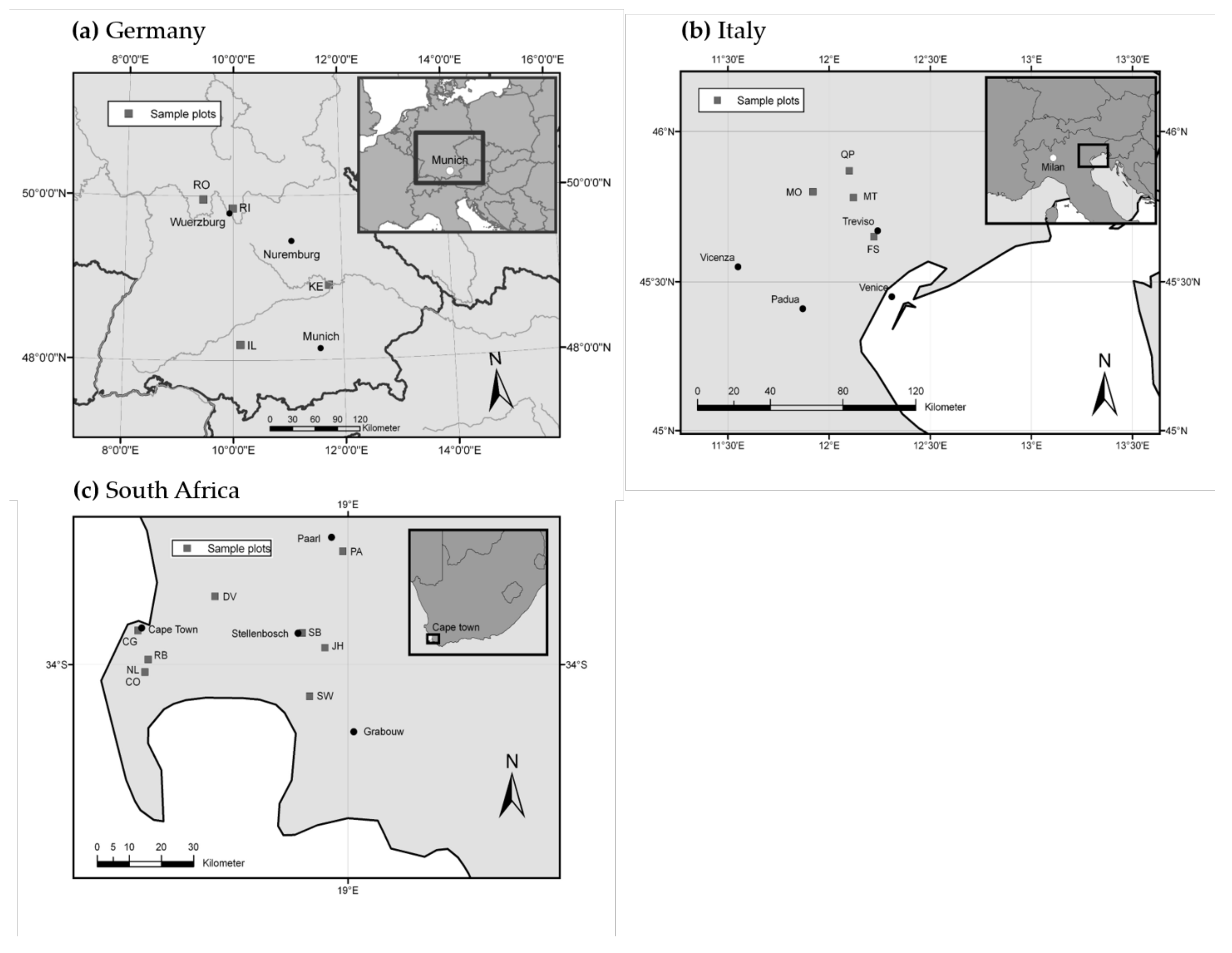
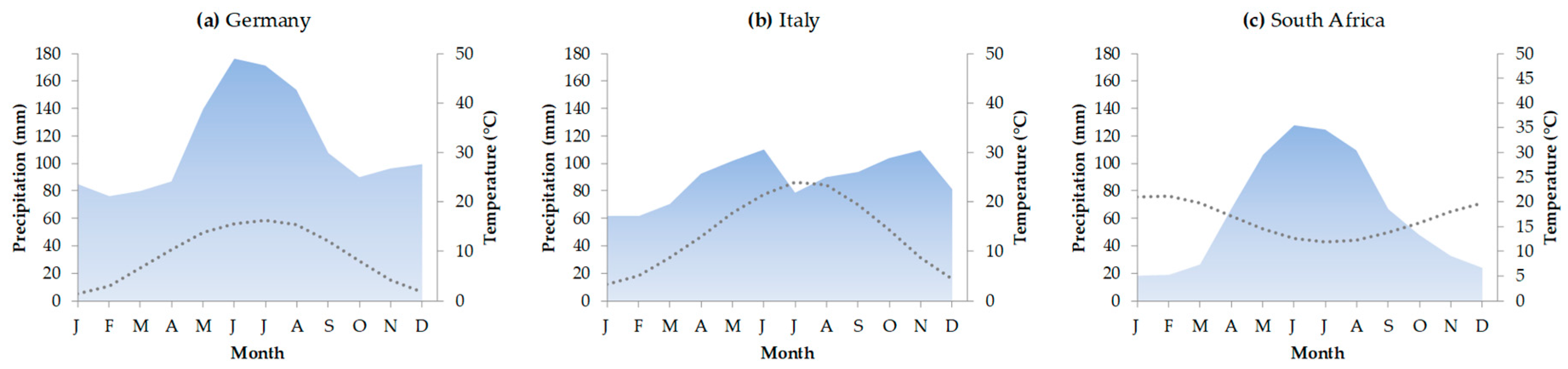
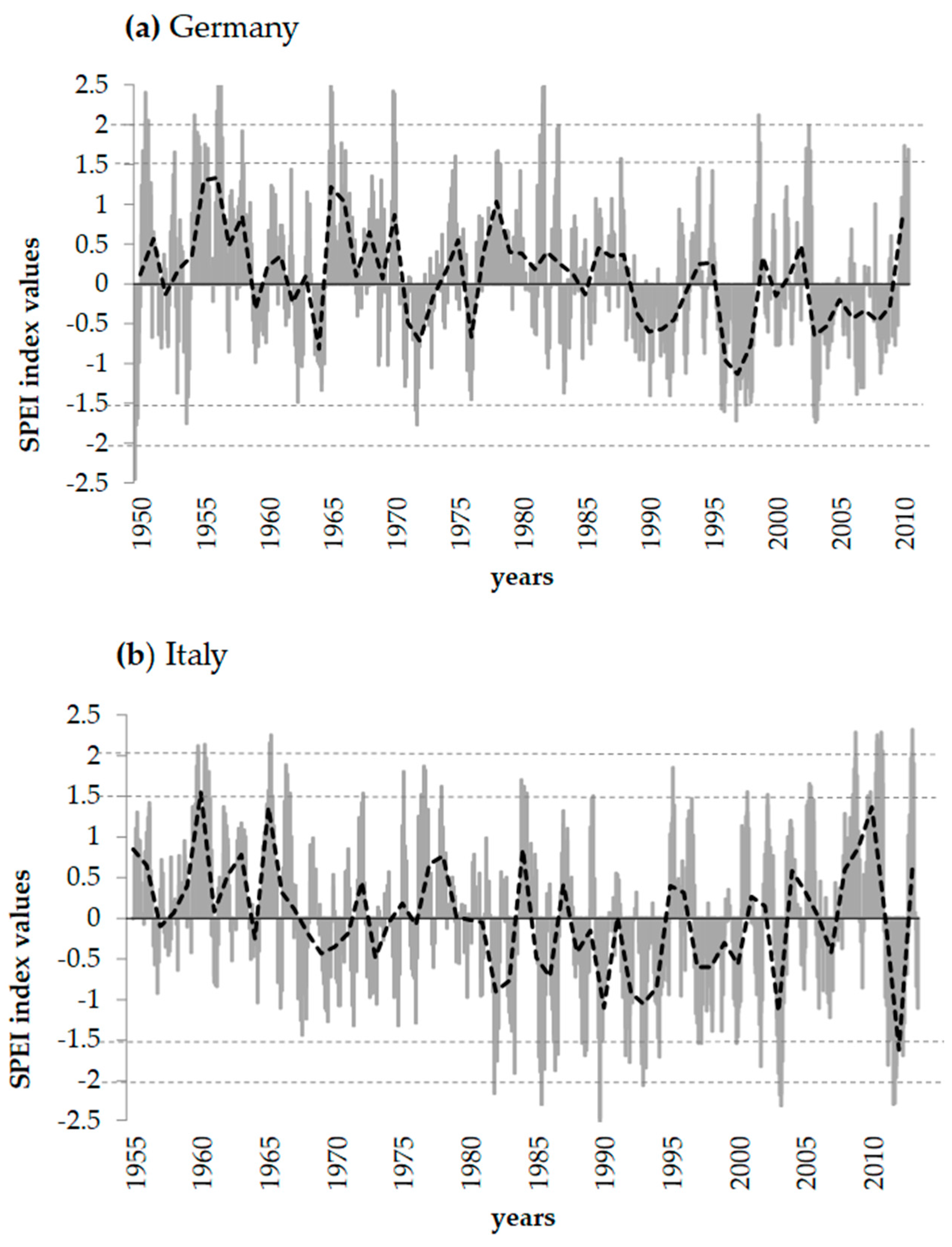
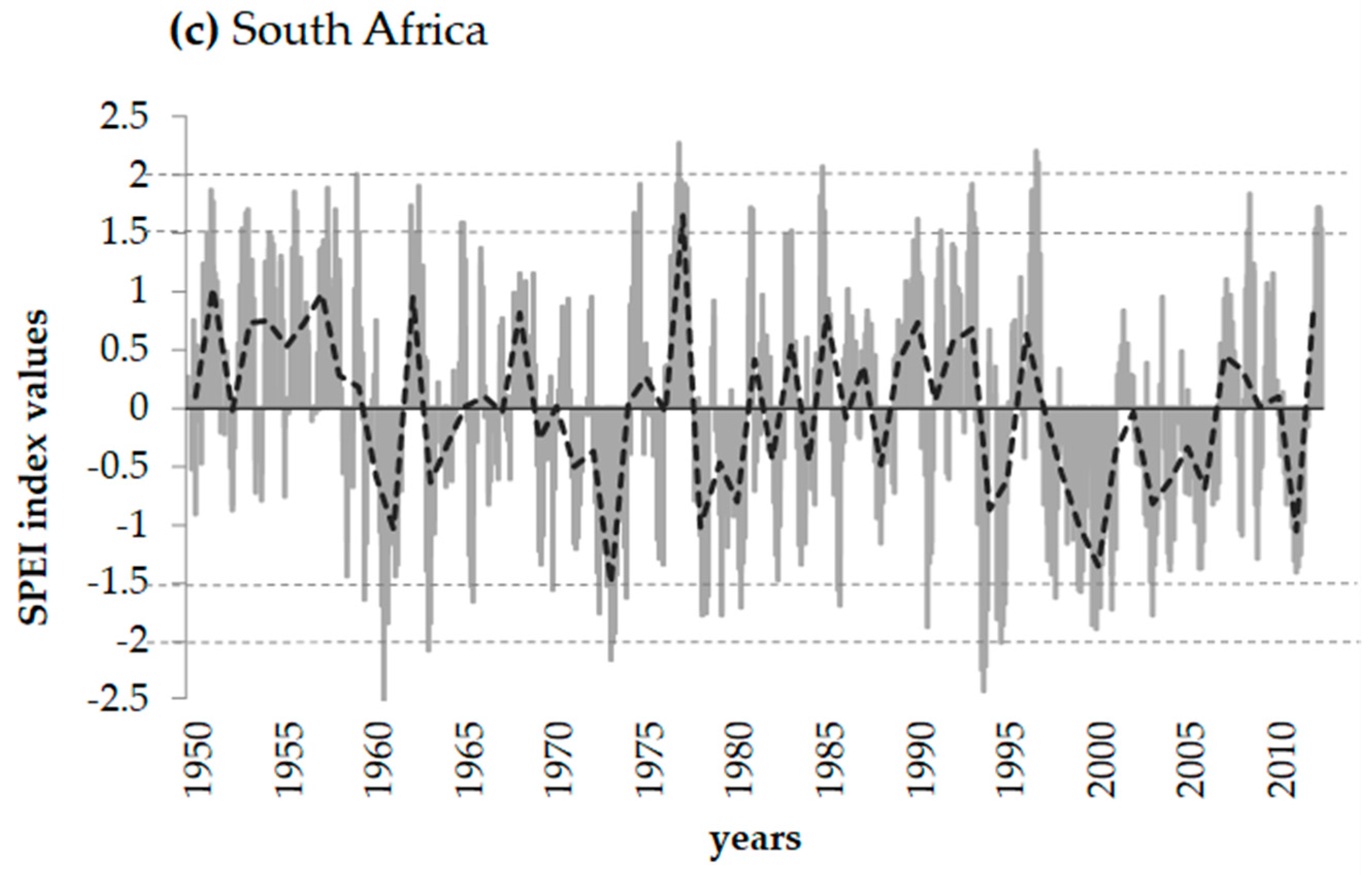
2.1. Study Areas and Climatic Conditions

The study sites are located in Southern Germany, Northeast Italy, and Western Cape, South Africa. Each study site (hereafter termed “experiment”) consists of different research areas within each country. For Germany and Italy, four sites were selected, while nine sites were designated in South Africa.

The four sites in Southern Germany are situated between 9°26′ E–11°48′ E and 48°11′ N–49°57′ N, covering North to South Bavaria (Figure 1a). A detailed description of these experiments can be found in Pretzsch et al. [28]. The German sites represent the temperate climate zone, where the annual mean temperature is within a range of 7.0–8.5 °C and the mean precipitation within 660–960 mm. The climate data for this data set was obtained from weather stations close to each of the four sites (Figure 2a) [29].

The chosen Italian sites were located in the Veneto region (Northeast Italy), with coordinates ranging from 45°52′ N–45°38′ N to 11°55′ E–12°07′ E (Figure 1b). This experiment represents the transition zone from warm-temperate to subtropical climate. Mean annual temperature ranges between 12.9–14.1 °C and mean annual precipitation varies around 590–800 mm/year (Figure 2b). Climate data for the Italian research sites were available in a monthly resolution from climate stations close to the research plot.

Both, the German and Italian study areas are located within the natural range of the species Quercus robur L./Qu. petraea Liebl. [27,30].

The study areas in the Western Cape, South Africa, represent growing conditions that are not typified by the natural occurrence of the chosen oak species. Research locations were selected within the Western Cape Province, in the districts of Cape Town and the Cape Winelands (coordinates 33°56′ S–34°08′ S/18°28′ E–18°97′ E). These sites represent oak growth in the Mediterranean climate zone of the Southern Hemisphere (Figure 1c). Mean annual temperature is substantially higher than in the natural distribution area of these species and vary around 16.0–17.1 °C, and the mean annual precipitation ranges within 450–830 mm (Figure 2c). Climate data were obtained from weather stations close to the plots.

2.2. Tree-Ring Data

For the experiments in Germany and Italy, pure oak stands were chosen. From each research site, we sampled solely dominant trees. The sampled trees in South Africa are primarily solitary grown oaks in rural areas around Cape Town, Stellenbosch, and Paarl. In total, 139 trees were sampled; 66 oaks from Germany, 20 from Italy, and 53 from South Africa were used for dendrochronological measurements and analyses.

Standard measurements of tree height and diameter at breast height (DBH) were recorded for all investigated trees. Trees were cored from two directions with an angle of 90° using a 5 mm increment corer (Haglöf, Langsele, Sweden). Thereafter, the cores were polished with progressively finer sandpaper from grit size 180 up to 800. Annual ring widths were measured with the Lintab measuring system using the TsapWin software (Rinntech, Heidelberg, Germany) [31]. Crossdating and synchronization of ring-width data was accomplished by the software TsapWin [31] and COFECHA [32,33] using standard dendrochronological methods. Chronologies of each experiment were built from a minimum sample depth of five trees. We removed the biological age trend in the ring-width data. A double de-trending procedure was applied to all series by using the Dendrochronology Program Library in R (dplR-package) [34,35]. The resulting index series contains only year-to-year variability associated with fluctuations in climate [36,37,38]. In this procedure, the raw ring-width series were conservatively standardized by adjusting a negative exponential or a linear regression function with negative slope. Thereafter, the resulting index values were de-trended by a smoothing cubic spline with a 50% frequency-response cut-off equal to 67% of the series length to calculate dimensionless ring-width indices (RWIs). To produce trend-eliminated time-series of the ring-width indices, in a final step, autocorrelation was removed using autoregressive (AR) models and the series were averaged using Tukey’s biweight robust mean. This reduces bias caused by extreme values. Through this procedure, the long-term growth trends in the raw tree-ring series were removed. Mean growth rate average and standard deviation, as well as expressed population signal (EPS), mean sensitivity (MS), and mean inter-series correlation (Rbar) were calculated for the chronologies using the dplR package in R [34,39,40]. EPS was used to test the population strength’s representation of the resulting tree-ring chronologies [41]. This was calculated on a 50-year running window with an overlap of 25 years [36,42] for the common period of each experiments’ tree-ring series. Mean sensitivity (MS) depends on the year-to-year variability and was employed as a measure for variability in the tree-ring series [38,40,43]. The mean inter-series correlation (Rbar) is a metric for agreement between all tree ring series to be averaged to a site chronology. It was calculated to assess the signal strength of the site chronologies [36,42,44] over the common period of each experiments’ tree-ring series.

2.3. Evaluation of Long-Term Growth Trends

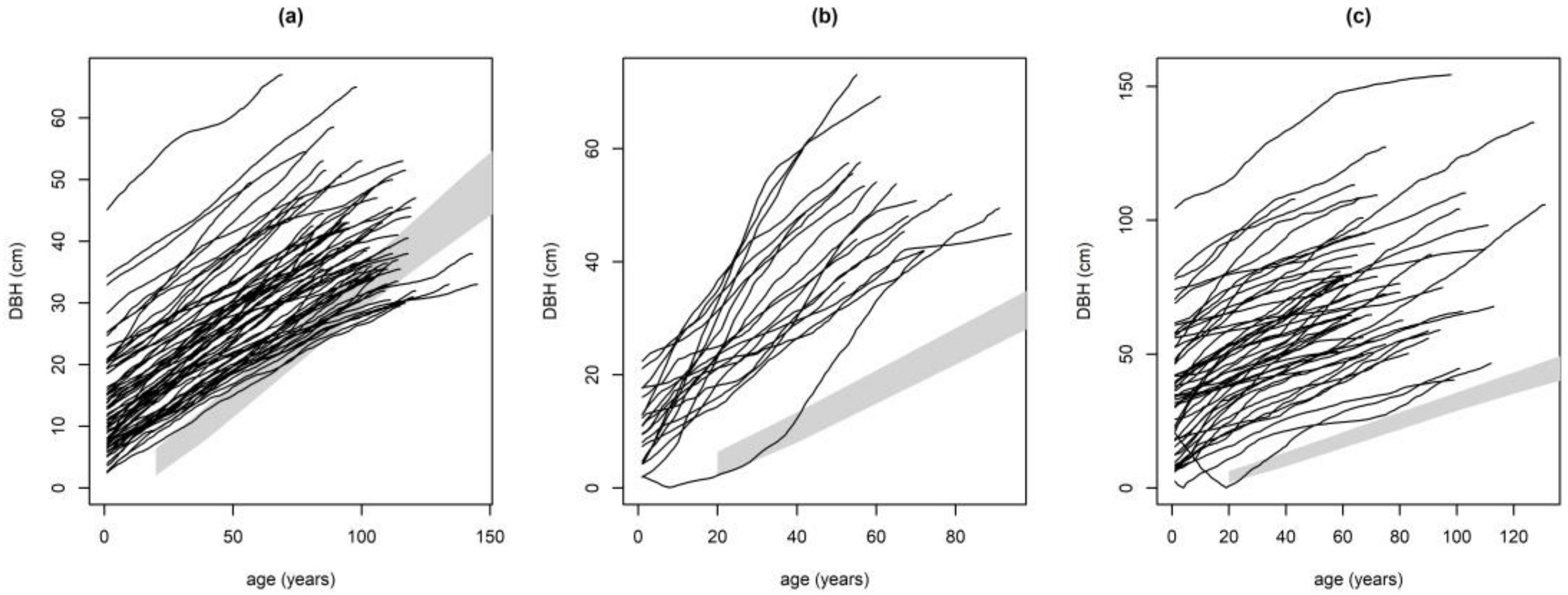
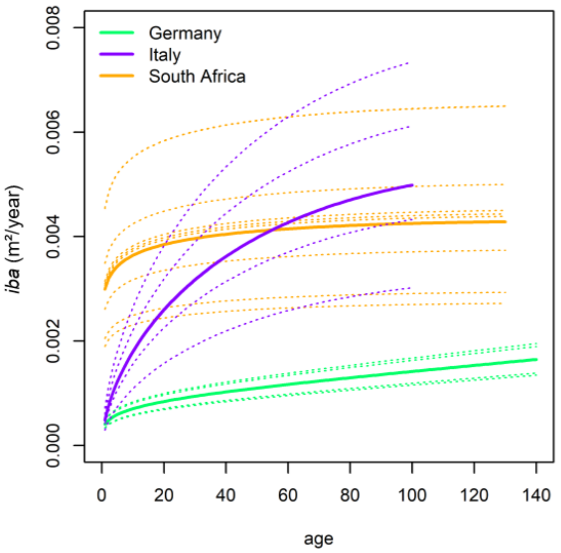
2.3.1. Performance of Growth Level within and beyond the Natural Range

Many studies have reported significant changes of tree growth due to environmental changes during the last decades [19,20,45,46,47,48]. Consequently, we analysed our data for recent growth trends by fitting a biologically plausible age-increment model to all tree ring data up to 1980. We extrapolated the fitted model beyond this cut-off and compared its predictions to the observed tree increments after 1980. We chose this year as a cut-off due to the length of the tree-ring data sets Therefore, we achieved a considerable length of tree-ring data from both periods (before and after 1980) for our long-term analysis. Assuming, in the null hypothesis, that variables have no influence on the age-increment relationship, we chose the Hugershoff equation for the age-increment model. The Hugershoff equation is, in addition to being biologically meaningful [49], easy to linearize and can therefore be handled with standard regression methods. We chose the individual tree basal area growth iba (m²/year) as our measure for tree increment because, in contrast to diameter increment, it directly represents information about biological production [50]. Applied to iba, the Hugershoff model reads as follows (Equation (1)):

$$iba=a_0·t^{ a_1}·{\mathrm{e}}^{ a_2·t},$$

(1)

where t is tree age and a₀, …, a₂ are constants (a₀, a₁ > 0, a₂ < 0).

In linearized form it can be written as (Equation (2)):

$$\ln \left(iba\right)=\ln \left(a_0\right)+a_1·\ln \left(t\right)+a_2·t,$$

(2)

This linearized form was fitted to all observations of tree age and basal area increment up to 1980 using the following linear mixed effects model (Equation (3)):

$$\ln (ib{a}_{ijkl})={\beta }_0+{\beta }_1·\ln \left(t_{ijkl}\right)+{\beta }_2·t_{ijkl}+b_i+b_{ij}+b_{ijk}+c_i·\ln \left(t\right)+d_i·t+{\epsilon }_{ijkl},$$

(3)

where the indexes i, j, k, and l represent the country, the study site, the individual tree, and an individual observation, respectively. The fixed effect parameters are β₀, β₁, and β₂. b_i, b_ij, b_ijk, c_i, and d_i are normally distributed random effects with an expected value of 0, and ε_ijkl are I.I.D. errors (independent and identically distributed errors). By adding to the fixed effect parameter β₀, the random effects b_i, b_ij, and b_ijk allow for a country-, study-site-in-country-, and a tree-in-study-site-specific scaling of the Hugershoff model. The random effects c_i and d_i in addition permit a general country-specific curve shape by adding to the fixed effect parameters β₁ and β₂. This model structure enabled us to perform biologically plausible model fits and predictions even for trees with short tree ring series, where simple individual tree model fits would not lead to useful results.

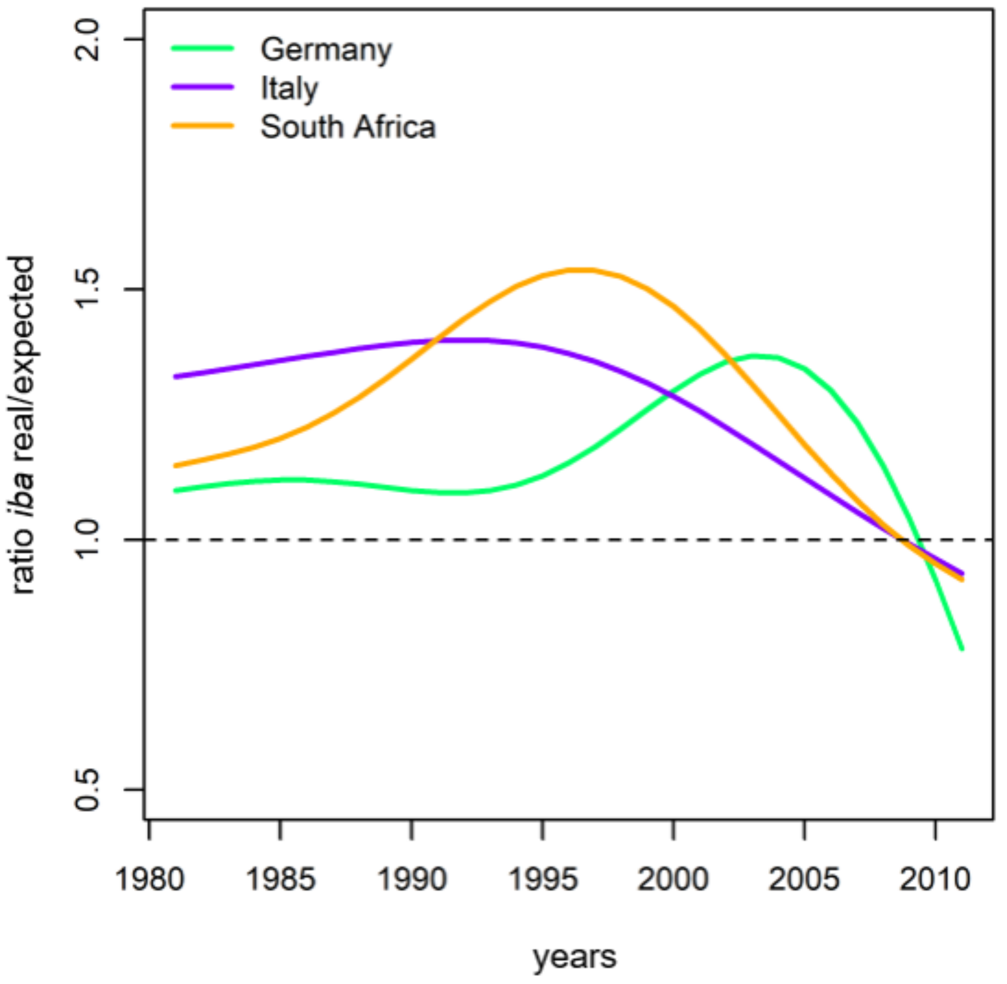
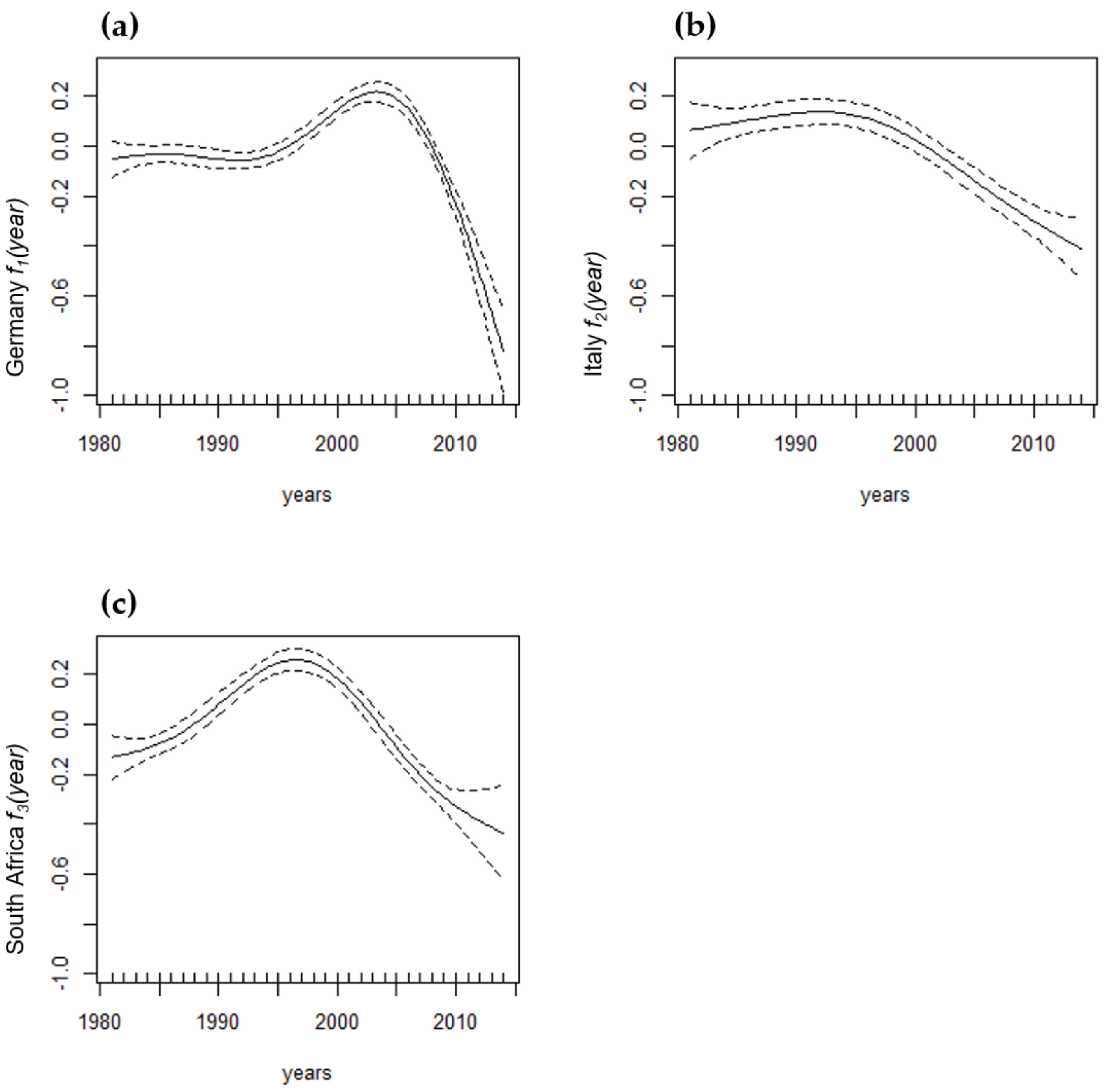
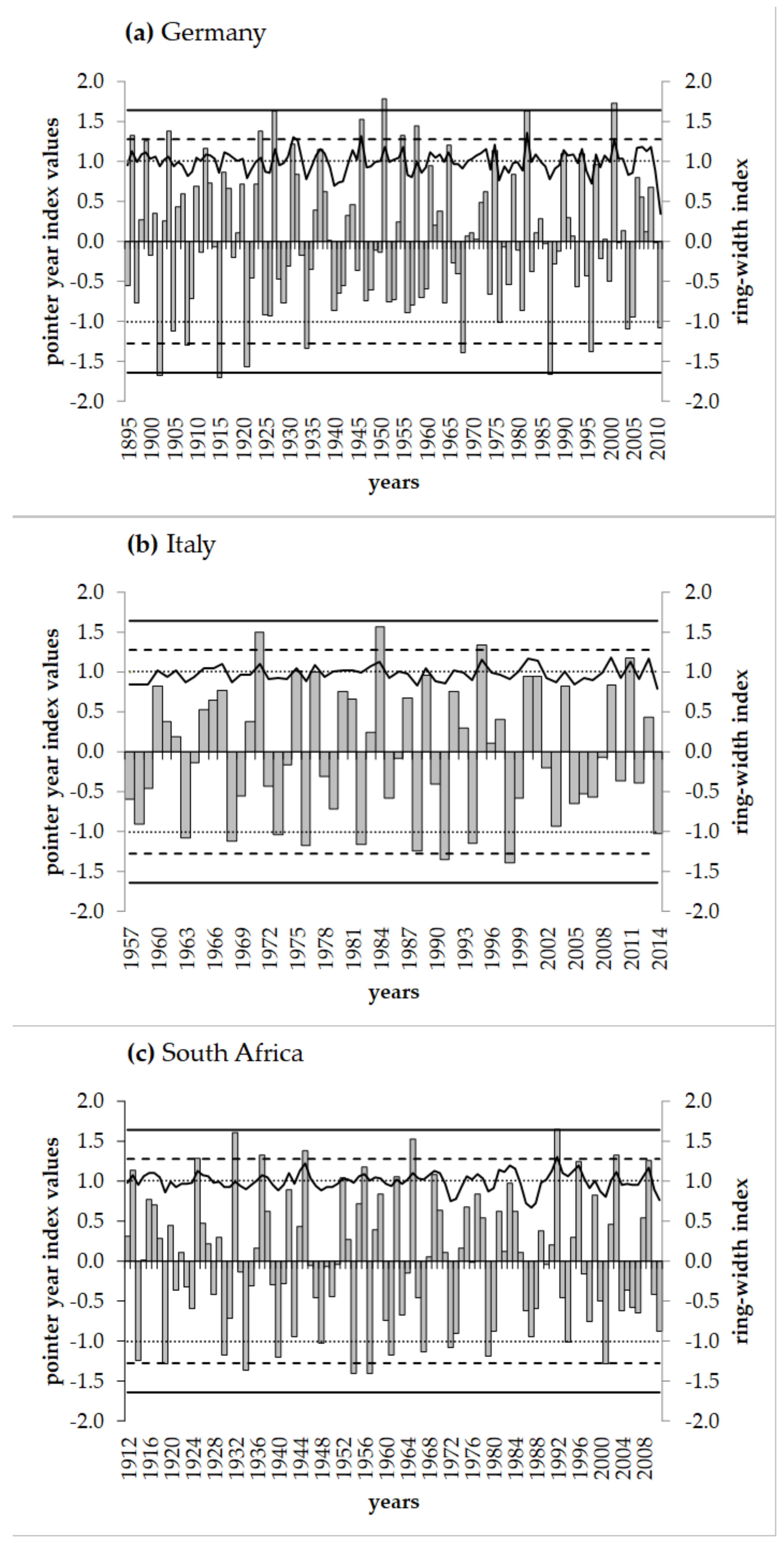
2.3.2. Long-Term Growth Behaviour and Recent Growth Trends

For all observations after 1980, we calculated the expected basal area increments ${\widehat{iba}}_{ijkl}$ by applying the fitted model from Equation (3) including all fixed and random effects. Dividing the actual basal area increments $rib{a}_{ijkl}$ by the expected ones, we obtained Equation (4):

$$rib{a}_{ijkl}=\frac{ib{a}_{ijkl}}{{\widehat{iba}}_{ijkl}},$$

(4)

This quantifies, for each single tree and for each year in the extrapolation period, how much the actual increment deviates from the one that would be expected if growth conditions were the same as in 1980 and earlier. In order to test for significant country-specific patterns in riba, we applied the following generalized additive mixed effects model (Equation (5)):

$$rib{a}_{ijkl}={\beta }_0+f_1\left(yea{r}_l\right)·a_{1_i}+f_2\left(yea{r}_l\right)·a_{2_i}+f_3\left(yea{r}_l\right)·a_{3_i}+ {\beta }_1·a_{2_i}+ {\beta }_2·a_{3_i}+b_{ij}+b_{ijk}+{\epsilon }_{ijkl},$$

(5)

The indexes in Equation (5) have the same meaning as in Equation (3); the same is true for the fixed effect β₀ and the random effects b_ij and b_ijk, and for the I.I.D. errors ε_ijkl. The functions f₁, f₂, and f₃ are non-parametric smoothers as functions of the calendar year (year); each one applies to a specific country—this is indicated by the binary coded variables a₁, a₂, a₃, which are defined as follows (Equations (6a)–(6c)):

$$a_{1_i}=\{\begin{array}{cc}1& if country i is Germany\\ 0& otherwise\end{array},$$

(6a)

$$a_{2_i}=\{\begin{array}{cc}1& if country i is Italy\\ 0& otherwise\end{array},$$

(6b)

$$a_{3_i}=\{\begin{array}{cc}1& if country i is South Africa\\ 0& otherwise\end{array},$$

(6c)

The fixed effects β₁ and β₂ allow for estimating country-specific base levels of riba in combination with β₀, because they are associated with the binary variables a₂ and a₃, which represents a dummy coding. Therefore, β₀ is the base-level prediction for Germany while ${\beta }_0+{\beta }_1$ and ${\beta }_0+{\beta }_2$ is the same prediction for Italy and South Africa, respectively.

All statistical computations were performed with the software R version 3.2.2 [51], specifically the packages lme4 [52] and mgcv [53].

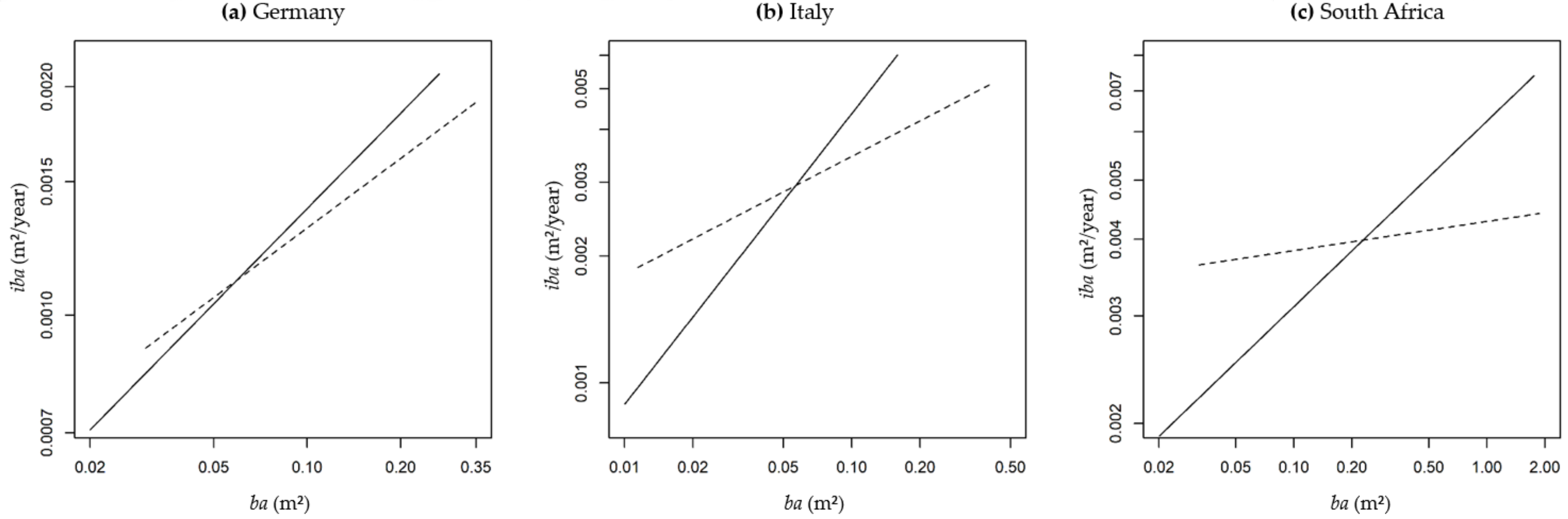
2.3.3. Change of Size-Growth-Relation During the Last Decades

For a tree growing under constant conditions, an allometric relationship (see below, Equation (7))

$$\ln \left(y\right)=a+b·\ln \left(x\right),$$

(7)

can be expected between its size x and its size growth y [54]. Consequently, any change in the parameters a and b of this relationship would indicate a change in the tree’s growing conditions. We utilized this concept for indirect testing of whether the growth conditions of the oaks were different in the years before and after 1980. Taking the tree basal area (ba) at a specific point in time as the size variable and the basal area increment in the subsequent year (iba) as the size growth variable, we formulated the following linear mixed-effect model (Equation (8)):

$$\ln \left(ib{a}_{ijt}\right)={\alpha }_0+{\alpha }_1·perio{d}_{ijt}+a_i+a_{ij}+\left({\beta }_0+{\beta }_1·perio{d}_{ijt}+b_i+b_{ij}\right)·\ln \left(b{a}_{ijt}\right)+{\epsilon }_{ijt},$$

(8)

The indexes i, j, and t represent the study site, the individual tree, and a specific point in time (calendar year), respectively. The variable period indicates whether an observation is from a year before (period = 0) or after 1980 (period = 1). The model’s fixed effect parameters are ${\alpha }_0$, ${\alpha }_1$, ${\beta }_0$ and ${\beta }_1$, while $a_i$, $a_{ij}$, $b_i$ and $b_{ij}$ are random effects on the study site level (index i) and on the tree-in-study-site level (indexes ij). These random effects are assumed to be normally distributed with an expectancy of 0. The same assumption can be made for ${\epsilon }_{ijt}$ which represents I.I.D. errors. If ${\alpha }_1$ and ${\beta }_1$ or both significantly differ from zero, this would indicate different allometric relationships before and after 1980.

The random effects in the model have important functions: $a_i$ and $b_i$ cover specific effects that result from the given site level combinations and thus allow for significant overarching relationships to be identified. The role of $a_{ij}$ and $b_{ij}$ is to cover autocorrelation effects due to repeated measurements from each tree. We considered it important to not only include random effects on the intercept of the allometric relationship (random effects $a_i$, $a_{ij}$) but also on the slope (random effects $b_i$, $b_{ij}$), which might differ considerably between study sites [55].

We fitted the mixed linear model (Equation (8)) for the whole dataset as well as separately for each climate zone (Temperate Germany, Warm-Temperate/Subtropical Italy, and Mediterranean South Africa). This allowed us to test for a general period effect (before and after 1980) on the size-growth-relation of oaks on the one hand. On the other hand, the zone-specific fits informed us in more detail without ending up with an over-complicated overall model. The range of tree basal areas in both periods, before and after 1980, largely overlaps. Thus, biased results due to unbalanced data had not to be suspected.

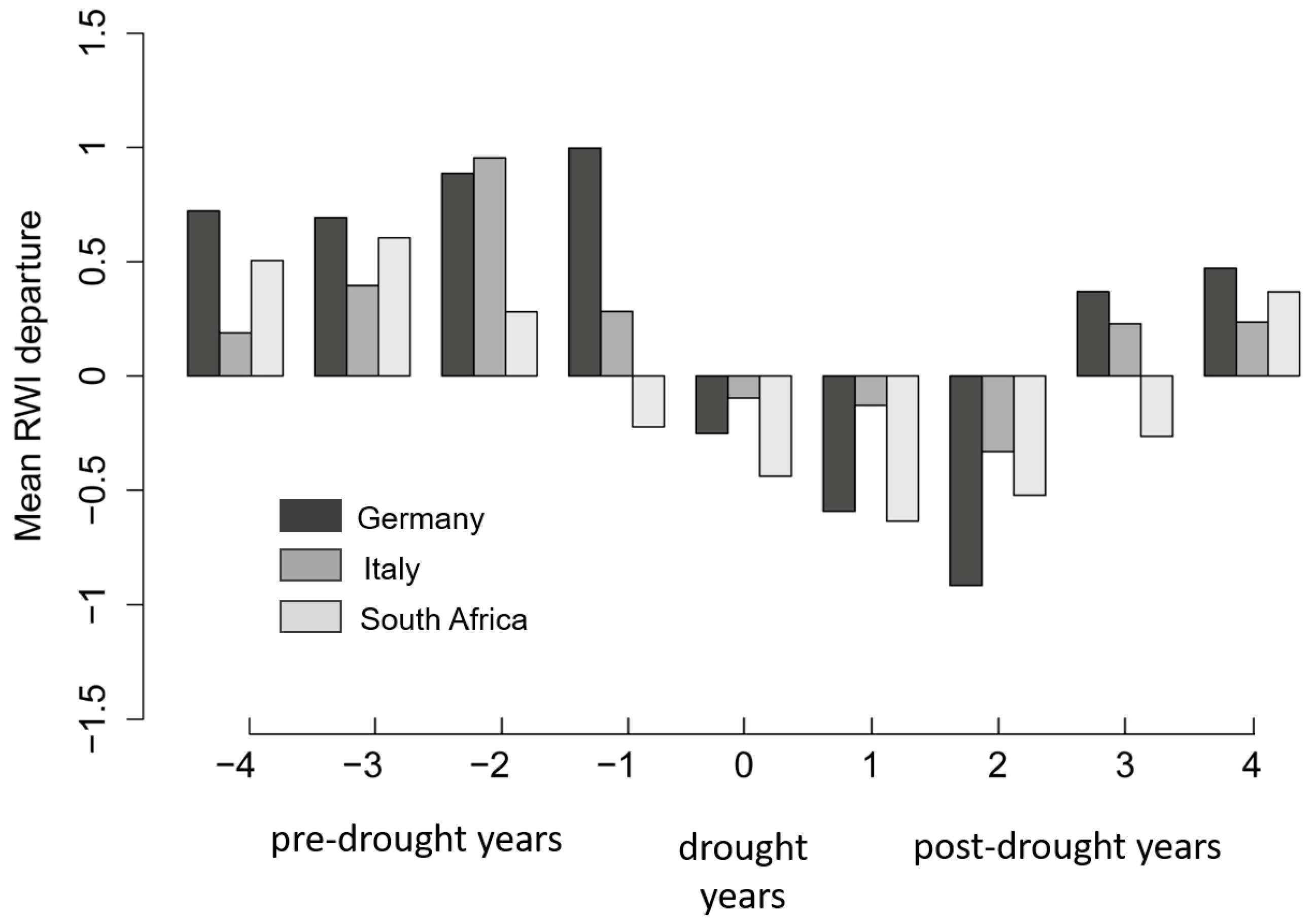
2.4. Reactions of Oak Growth on Drought Events

To ascertain whether extreme event years are appearing in all experiments and the differentiation in strength of these events, we applied pointer year analyses to the data sets [56,57].

In a first step, all raw time-series were standardized, for this analysis, with their 13-year moving average [57]. In a second step, these time-series were normalized to a standard deviation of one and a mean of zero over the period 1956–2004 for Germany, 1946–2009 for Italy, and 1903–2005 for South Africa [56]. This procedure enables an identification of growth anomalies to the probability density function of the standardized normal distribution and facilitates a clear assignment of the normalized Cropper values (C) as follows: weak for (C) > +1.000/−1.000, strong for (C) > +1.280/−1.280, and extreme for (C) > +1.645/−1.645 [56]. Secondary to climatic factors, additional matters exist that can cause pointer years, including fruiting, masting behaviour, and insect outbreaks.

This study employed the standardized precipitation evapotranspiration index (SPEI) as a drought indicator to determine the occurrence and extent of drought events and periods in South Germany, Northeast Italy, and the Western Cape, South Africa. To analyse the reaction on drought events comparing oak growth within and outside their natural distribution area, we calculated a drought index for the three experiments (Germany, Italy, and South Africa) using the available climate data from each country/experiment. Since drought is determined by temperature, rainfall, and evaporative changes, it is important to consider each variable individually in order to accurately analyse its impact. Vicente-Serrano et al. [58] proposed a drought index: SPEI, which depends on the potential evapotranspiration (PET). SPEI accounts for the effect of temperature variability in drought monitoring, and it can be computed at different time-scales. The process of calculating SPEI is based on a monthly balance between precipitation and PET, which is adjusted using a three-parameter log-logistic distribution to take into account common negative values [59]. PET was calculated using the Thornthwaite [60] equation. It is a simple method used to compute monthly potential evapotranspiration, when, as is the case here, only temperature data are available. For this study, we calculated the SPEI with a time scale of 6 months for Germany from 1947–2011, for Italy from 1955–2012, and for South Africa from 1945–2011.

The resulting drought years attained from the SPEI evaluations for each experiment were further analysed. For this, we applied superposed epoch analyses (SEAs) [61,62] to the ring-width data of the measured oaks in order to examine whether drought events have an influence on the growth of oak and how this varies in different climates. One point of interest was the recovery time after drought events with different intensities. In a first step, we removed the biological age trend in the ring-width data, following the same method as described under Section 2.2. In a second step, we averaged the difference between the mean ring-width index of each tree and the corresponding average value for the, in total, 9 years (4 years before the event year, the event year itself, and 4 years after the event year), respectively. Bootstrap resampling was used to determine whether RWIs for these years were significantly different to a random set of other years (lag: +1 year) from the data set. Bootstrapping conduces in the significance test for the derivation of confidence intervals (p < 0.05), for which the dendrochronological package dplR was used [39].

3. Results

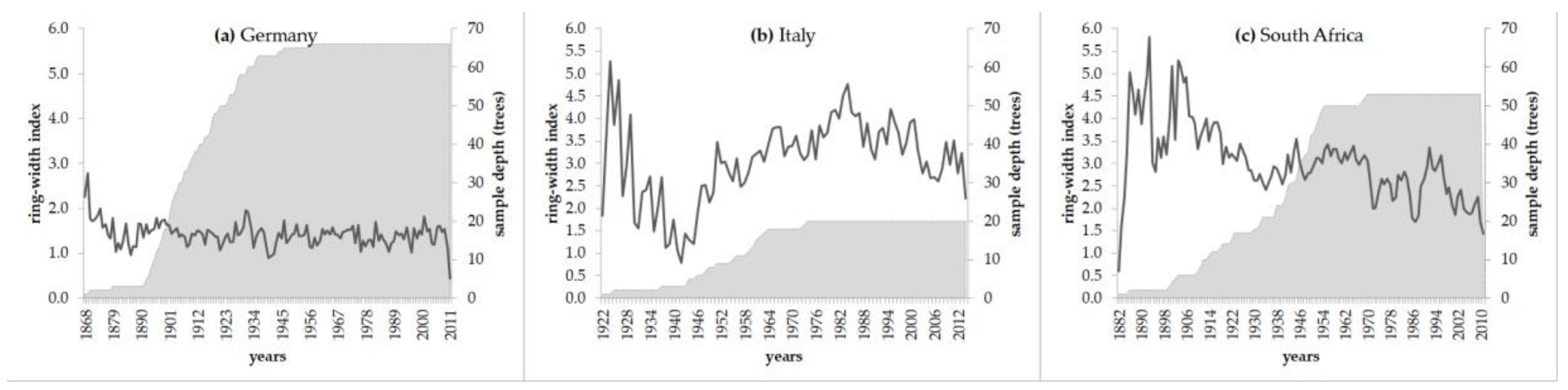
3.1. Tree-Ring Data and Their Basic Statistics

The selected trees at the four German, the four Italian, and the nine South African research sites covered a representative scope of age, height, and diameter at breast height (DBH) (

Table 1. Overview of sampled trees at each study site and standard parameter for the ring-width chronologies.

Study Site	Germany
	Value
		Average	Std. Dev. (Standard Deviation)	Min	Max
Overall timespan	1868–2011
Common interval	1956–2011
Mean growth rate (mm a−1)		1.38	0.56	0.15	4.74
Expressed population signal (EPS)	0.947
Mean sensitivity (MS)	0.276
Mean inter-series correlation (Rbar)	0.234
Diameter at breast height (cm)		41.48	8.18	29	67
Tree height (m)		30.13	2.91	24.1	37.5
Study Site	Italy
	Value
		Average	Std. Dev.	Min	Max
Overall timespan	1922–2014
Common interval	1974–2014
Mean growth rate (mm a−1)		3.34	1.87	0.25	10.62
Expressed population signal (EPS)	0.776
Mean sensitivity (MS)	0.349
Mean inter-series correlation (Rbar)	0.148
Diameter at breast height (cm)		51.98	9.05	36.4	73.1
Tree height (m)		28.66	5.28	18.2	39.7
Study Site	South Africa
	Value
		Average	Std. Dev.	Min	Max
Overall timespan	1882–2011
Common interval	1970–2010
Mean growth rate (mm a−1)		2.74	1.68	0.29	12.48
Expressed population signal (EPS)	0.927
Mean sensitivity (MS)	0.216
Mean inter-series correlation (Rbar)	0.193
Diameter at breast height (cm)		76.8	25.18	36.3	154.4
Tree height (m)		16.51	4.43	19.75	27.9

). Tree-ring series from all sites of each country were successfully cross-dated, resulting in the establishment of three chronologies. For each experiment’s chronology, the basic tree ring statistics are shown in Table 1, according to their equivalent periods.

Matching the extent of increment growth (mean growth rate, Table 1) between the three research areas, we observed higher ring-width variability for the trees in Italy and South Africa compared to the trees from Germany (Figure 3). Compared with trees in Germany, which had a maximum growth rate of 4.75 mm a⁻¹, oaks in Italy showed a growth rate of 10.62 mm a⁻¹ and oaks in South Africa a rate of 12.48 mm a⁻¹. Differences in ring-width variability could also be seen when matching the level of raw ring-width data (Figure 3) between the three experiments.

Mean sensitivity (MS) and mean inter-series correlation (Rbar) values were similar at the German and South African research sites and range within the threshold values given by Speer [63], whereas at the Italian research sites, MS showed the highest value but Rbar the lowest. EPS values, calculated for the common periods, respectively, revealed the highest value for the German sites. The EPS value for South African oak trees was just a little bit lower, whereas Italian oaks once again showed the lowest value (Table 1).

3.2. Evaluation of Long-Term Growth Trends

Performance of Growth Level within and beyond the Natural Range

A first overview comparing the growth level of oaks within and outside their natural distribution area is shown in Figure 4 (derived from model Equation (3); model parameters can be found in the Appendix A

Table A1. Model parameters for the linear mixed effect model Equation (3) displaying the performance of growth level (Figure 4). Parameter estimates for each experiment’s fixed effects with standard errors (Std. Error) and significances (p) and the standard deviation (Std. Dev.) of random effects. Estimated country-specific values were added to the random effects, as they are needed for the curve display in Figure 4.

Fixed effects		Parameter	Estimate	Std. Error	p
		${\beta }_0$	−6.8817	0.5538	0.0000
		${\beta }_1$	0.1465	0.0286	0.0000
		${\beta }_2$	0.0087	0.0074	0.0000
Random effects		Parameter	Std. Dev.
		$b_{ijk}$	0.4535
		$b_{ij}$	0.3690
		$b_i$	0.9399
		$c_i$	0.0415
		$d_i$	0.0127
		${\epsilon }_{ijt}$	0.3912
	Estimated country-Specific Values
		Parameter	Germany	Italy	South Africa
		$b_i$	−0.7810	−0.2355	1.0166
		$c_i$	0.0187	0.0220	−0.0408
		$d_i$	−0.0050	0.0143	−0.0093

). It clarifies whether long-term growth trends have different characteristics. Comparing the three experiments, the basal area increment development over age is at the lowest level for the oaks in Germany. The Italian oak trees showed the fastest increase in basal area development over age. South African oaks start at the highest level but then increase only slightly with age, i.e., they have a similar development pattern with increasing age as the German oaks. The dotted lines in Figure 4 represent the model Equation (3) results for the regions within the experiments, respectively. South Africa and Italy revealed higher site-specific variability than Germany did.

To study the long-term growth of oaks, we proposed a cut-off of the data set in 1980. Thus, we looked at a basal area growth development for the period before and after 1980 for all experiments (Figure 5, derived from model Equation (8); model parameters found in the Appendix A

Table A2. Model parameters for the linear mixed effect model Equation (8) displaying the change of size-growth relation (Figure 5). Parameter estimates for each experiment’s fixed effects with standard errors (Std. Error) and significances (p) and the standard deviation (Std. Dev.) of random effects.

Germany
Fixed effects		Parameter	Estimate	Std. Error	p
		${\alpha }_0$	−5.6240	0.1466	0.0000
		${\beta }_0$	0.4170	0.0408	0.0000
		${\alpha }_1$	−0.3183	0.0664	0.0000
		${\beta }_1$	−0.1127	0.0288	0.0000
Random effects	Level	Parameter	Std. Dev.
	Plot	$a_i$	1.1782
	Plot	$b_i$	9.1077
	Tree in plot	$a_{ij}$	1.0198
	Tree in plot	$b_{ij}$	0.3064
	Residual	${\epsilon }_{ijt}$	0.3405
Italy
Fixed effects		Parameter	Estimate	Std. Error	p
		${\alpha }_0$	−3.8436	0.2453	0.0000
		${\beta }_0$	0.6911	0.0369	0.0000
		${\alpha }_1$	−1.1793	0.1384	0.0000
		${\beta }_1$	−0.4106	0.0495	0.0000
Random effects	Level	Parameter	Std. Dev.
	Plot	$a_i$	0.4091
	Plot	$b_i$	5.4971
	Tree in plot	$a_{ij}$	0.2442
	Tree in plot	$b_{ij}$	0.3220
	Residual	${\epsilon }_{ijt}$	0.4468
South Africa
Fixed effects		Parameter	Estimate	Std. Error	p
		${\alpha }_0$	−5.0762	0.0710	0.0000
		${\beta }_0$	0.3033	0.0219	0.0000
		${\alpha }_1$	−0.3774	0.0330	0.0000
		${\beta }_1$	−0.2556	0.0241	0.0000
Random effects	Level	Parameter	Std. Dev.
	Plot	$a_i$	0.3023
	Plot	$b_i$	3.5391
	Tree in plot	$a_{ij}$	0.3023
	Tree in plot	$b_{ij}$	0.0217
	Residual	${\epsilon }_{ijt}$	0.5122

). The growth trend follows a similar pattern at all sites but with different magnitudes. It appears small trees are growing faster than historical trends until they reach a certain size threshold, and larger trees tend to grow more slowly than historical trends (Figure 5). At all three experiments the slopes in basal area increment are significantly different when the periods before and after 1980 are contrasted. German oaks have the least growth change before and after 1980. On the Italian sites, the incremental gap between growth before and after 1980 is extensive. Oak growth has the steepest slope before 1980 starting at an individual tree basal area (m²) under 0.01 m² until 0.12 m² and flattens in the period after 1980. Looking at the growth of oak trees in South Africa, the slope between basal area increment, before and after 1980, differs considerably. The crossover point (before/after 1980) is at about 0.06 m² in Europe but at 0.20 m² in South Africa. As such, moderate-sized trees (ba = 0.10 m²) in South Africa currently grow faster, as opposed to the same size of trees in Europe, which grow slower than historic rates.

Significant differences between the experiments are found by observing whether oak growth is of a variable pattern by focusing on the long-term development. Figure 6 (derived from model Equation (5); model parameters in the Appendix A

Table A3. Model parameters for the generalized additive mixed effects model Equation (5) displaying the long-term growth behaviour and recent growth trends (Figure 6). Parameter estimates for each experiment’s fixed effects with standard errors (Std. Error) and significances (p) and the standard deviation (Std. Dev.) of random effects. The non-parametric smoothers as function of the calendar year are added to the fixed effects and are displayed in Figure A1 in the Appendix A.

Fixed effects		Parameter	Estimate	Std. Error	p
		${\beta }_0$	1.1494	0.1914	0.0000
		${\beta }_1$	0.1114	0.2961	0.7070
		${\beta }_2$	0.1309	0.2507	0.6020
	Non-parametric smoother				p
		f1(year) see Figure A1			0.0000
		f2(year) see Figure A1			0.0000
		f3(year) see Figure A1			0.0000
Random effects		Parameter	Std. Dev.
		$b_{ij}$	0.3508
		$b_{ijk}$	0.6122
		${\epsilon }_{ijt}$	0.4764

and Figure A1) shows the ratio values (after 1980) of the individual tree basal area increment growth, comparing real to expected growth, between the three experiments Germany-Italy-South Africa.

Expected growth as predicted by the growth model (Equation (5), calculated with values before 1980) would level out around a ratio of 1.0 on the Y-axis. Growth of oak trees in Germany seems to be quite close to the model prediction values. Although the level is mostly below that of the warmer sites, it does show an increase during the period 1997–1998 until 2003–2004. The trees in Italy indicate a higher growth than expected in the period after 1980 compared to the growth model before 1980. Compared to the other study sites, growth starts here on the highest level but decreases after 1995. Trees in South Africa indicate a slightly higher growth after 1980 than expected from the historic model. An increase in growth is visible from around the year 1990 until 1997–1998.

3.3. Reactions of Oak Growth on Drought Events

Pointer year analyses were applied to all data sets to examine the impact of extreme events on the growth of oaks grown in different climates. The pointer year totals for Germany (1895–2010) are 12 negative and 18 positive; for Italy (1957–2014), we found 10 negative and 6 positive; and for South Africa (1912–2010), 14 negative and 14 positive pointer years were observed.

Oaks at the German research sites had the strongest and most extreme negative pointer years in the time span 1900–1930. Two extreme positive and three extreme negative pointer years could be identified (Figure 7). On average, there are 1–2 negative pointer years and 2–3 positive pointer years (from weak to extreme per definition) that occur every century. On Italian research sites, no extreme pointer year was found in our data. However, from 1957 to 2012 there are two strong negative and three strong positive pointer years (Figure 7). South African oaks showed an equal ratio of negative to positive pointer years. Just one extreme positive pointer year was identified, in addition to six strong positive and five strong negative ones (Figure 7). On all sites, negative and positive pointer years are evenly balanced.

Identified pointer years were matched with their congruence to a drought index with annual resolution. Pointer years did not reveal an exact correlation to the identified drought years.

To identify drought years at each experiment, we chose the standardized precipitation evapotranspiration index (SPEI). According to Potop et al. [59], resulting negative and/or positive index values can be classified according to seven classes of SPEI categories, which range from moderate wet/dry over normal to severe and extreme wet and/or dry. In our approach, we chose two of these categories to differentiate extreme from severe droughts. A SPEI value of −2 to −1.5 is classified as severe drought and values ≤ −2 as extreme drought events (Figure 8).

Climate data showed no extreme drought years according to SPEI at the German research areas. Severe dry years were identified in 1953, 1972, 1997, and 2003. Of all the experiments, the Italian study sites had the most severe and extreme dry years. These were 1982, 1986, 1990, 1993, 2003, as well as 2012. Looking at the selected South African study areas, the years 1960, 1973, and 1994 could be identified as extreme drought events. Furthermore, several severe drought events were evident from 1960–2010 (Figure 8). Besides the drought events, we also identified drought periods for our study sites in South Africa (e.g., 1997–2000) whose effects were also reflected in the long-term analysis. For all experiment sites, the amount of drought events and/or periods increased from 1980 onwards, which reinforced our decision to set 1980 as a cut-off date for our long-term analysis (Figure 5 and 6). Calculations of the SPEI indicated several drought years per research area, which could be used in the superposed epoch analyses (SEA). For calculating SEA, we chose drought years that appeared in the SPEI analyses as either severe or extreme drought years. Furthermore, to minimize bias, we excluded years that were less than four years apart. Drought years occurring outside the common period (Table 1) of the research site’s tree-ring chronology were also excluded. In total, three to four drought years per experiment were incorporated into the analyses. For the oak chronologies from Germany, we chose the drought years 1972, 1997, and 2003; for the Italian sites, we selected the years 1982, 1986, 1990, and 2003; for South African oak trees, the drought years 1960, 1973, and 1994 were selected.

Oaks at each site showed a reduction and recovery phase after drought, but intensity and time were different between the experiments (Figure 9). All sites displayed the highest growth reduction two years after the drought event. This fact is most pronounced in the German experiment. Oaks growing on South African sites had the longest recovery time.

When comparing the three experiments, oak chronologies from Germany showed the strongest growth setback after a drought event. In the drought year itself, decline was minimal on all sites. In the first and second year after the drought, the majority of the trees experienced a setback in growth, whereas oaks on the Italian research sites showed the least reaction after a drought event. Based on the chosen drought years, oaks on the South African study sites indicated the strongest decline in the second year after a drought (Figure 9). Results revealed a high tolerance of water deficits for oaks on all research sites, as none of the experiments’ trees showed significant growth decline in the drought year itself nor in the following years. Mean RWI departures were also calculated for each site within the three experiments, these results are plotted in the Appendix A (

Table A4. Superposed epoch analysis for each region within the experiments Germany, Italy, and South Africa, respectively. Mean RWI departures are listed for the pre-drought years (−4 to −1), the drought years itself (0) and the post drought years (1 to 4).

Site	Years
	−4	−3	−2	−1	0	1	2	3	4
	Pre-Drought Years				Drought Years	Post-Drought Years
Germany
IL	0.55629803	−0.03131591	0.91157843	0.48650042	0.37747352	−0.40987714	−0.34604707	0.3198875	0.35851158
KE	0.23774573	0.40799534	0.07888110	0.69931780	−0.36785892	−0.15835306	−0.81287509	0.77624272	1.0969131
RI	0.47632093	0.69020222	0.75826215	1.0784091	−0.66902923	−0.89093999	−0.76053921	−0.03171566	0.00048237
RO	1.05106777	0.69237553	0.93242868	0.64102589	−0.00791415	−0.29594034	−0.85371995	0.24127894	−0.09626109
Italy
FS	0.17592635	0.47263100	0.66785080	−0.09426894	0.26321477	0.35170359	−0.29685685	0.43268679	0.49510446
MT	−0.09948952	−0.43667626	0.37670988	0.35216058	−0.07425614	−0.06914289	−0.17069694	−0.43803122	−0.41282043
MO	0.36724712	1.4248831	1.29156969	−0.06582161	−0.17323267	−0.84175735	−0.61972081	0.68742789	−0.19081160
QP	−0.1130041	−0.3646164	0.9829210	0.5270011	−1.0304076	−0.4681115	−0.3114193	−0.1379355	0.5459765
South Africa
RB	−0.15392203	−0.19508340	1.09611125	−0.02774566	−0.25770315	−1.04564693	0.626315598	−0.001743126	−0.307411933
SW	0.09559793	0.81468107	−0.01210531	−0.09462245	−0.21608670	−0.36220396	−0.58564310	−0.41582023	0.42060171
JH	0.62226984	0.04366845	0.06405663	−0.15354578	−0.16597562	−0.52549416	−0.38744865	0.07184230	0.26197139
PA	0.67328311	0.56504161	−0.42335109	−0.48853342	−1.0279399	−0.92447381	−0.00649988	0.70648546	0.03965515
SB	0.49508870	0.27462479	0.78459160	−0.46170574	0.03104207	−0.57616940	−0.86129925	−0.26494444	−0.03688565
DV	−0.11743943	0.96822879	0.00946096	−0.08080230	−1.0062275	−0.20950409	−0.27623300	−0.31475344	0.03968543
CG	0.72068534	0.78664249	0.40765661	−0.13206849	−0.79011497	−0.81164017	−0.07628534	−0.14777659	0.38371760
NL	0.3090942	11.867.157	−0.5120751	−0.4253017	−0.3917846	−0.5892783	−0.4236440	0.1466858	0.5765544
CO	0.4886513	0.0296665	0.2186459	0.1438576	−0.2926300	−0.2974016	−0.4423230	−0.6742106	0.2710374

IL: Illertissen; KE: Kehlheim; RI: Rimpar; RO: Rothenbuch; FS: Piombino Dese; MT: Valpago del Montello; MO: Monfumo; QP: Moriago della Battaglia; RB: Rondebosch; SW: Sommerset-West; JH: Jonkershoek; PA: Paarl; SB: Stellenbosch; DV: Durbanville; CG: Oranjezicht; NL: Newlands; CO: Constantia.

).

4. Discussion

Changing climate conditions will likely affect tree growth and have motivated forest science to identify possible pathways of growth reactions to facilitate adaptation. During the last decades, a wide range of studies have focused on the growth dynamics of trees within their natural habitat [23,65,66]. Other studies investigated tree growth response to climate change by looking at tree growth in regions that currently exhibit climate conditions that are expected for the area of interest under future climate [67,68,69,70]. Both approaches have the limitation that the real flexibility of a tree species against climate conditions is not fully covered. So far, species growing at conditions that are distinct from their natural range conditions rarely have been investigated. However, such studies could provide an idea of how native trees grow if climatic conditions are changing. Pretzsch et al. [71] showed, for trees growing under urban conditions, that growth could even be fostered due to higher temperatures. In our study, we included oaks growing at sites that exhibit natural range growing conditions as well as strongly diverging conditions. We have the advantage to revert to a data set of more than 100-years tree growth within and outside the trees natural range.

4.1. General Growth Level and Growth Trends

For the growth of oaks, the current study points out a lower variability in ring-width data for German oaks compared to the oak trees growing in the examined study sites in Italy and South Africa. Hereby, the year-to-year variability (Figure 3) and the general level of growth appears to be accelerated (Figure 4) for the trees that are growing in a warmer climate with possibly longer drought periods. The growth level of oaks growing at average temperatures of 11 °C (Italy) or 16 °C (South Africa) but at similar precipitation regimes as in Germany show a two and four times higher productivity respectively than those in Germany. Growth trajectories for all sites are far beyond those predicted by the existing yield table. Considering that all our results are based on a single tree level, we cannot provide any statements for stand level, where smaller trees would also be included. Higher temperatures, either through climate change or through generally effective climate conditions (Italy and South Africa), might explain the departure of growth trajectories from the yield table, which was developed for German growing conditions (Figure 10).

Even if we assume that for the study sites in South Africa the trees had more favourable conditions through possible tending activities like irrigation and reduction of competing vegetation, the long-term growth development seems to be more related to prevailing climate conditions. Relatively warm spring seasons, higher temperatures throughout the year, as well as an extended vegetation period potentially foster growth.

At all sites, a more rapid growth during the last decades (after 1980) was observed. Changes in size-growth relations (Figure 5) suggest that younger trees are currently growing quicker in diameter, but increment rates for older trees seem to be damped compared to before 1980. Consequently, for the trees investigated in our study, the general growth curve seems to be modified by one that has a steeper slope and an earlier inflection point. (Figure 11). This change in growth pattern appears to be most pronounced within oak trees in South Africa.

The accelerated growth can be traced by the comparison of recent growth level with that before 1980. Trees are currently performing better than they did before 1980 (Figure 6). Decreasing relation over time between modelled growth rates (before 1980) and observed growth rates, as visible from all three countries from 2009–2010 onwards, might be related to approaching growth curves through aging of the sampled trees. For the sampled oak trees from South Africa, the drop in the curve found around 1997–1998 could be exaggerated by the coinciding Super El Niño event in 1997–1998. That Super Nino event had a huge negative impact on the rainfall and temperatures in the Western Cape, South Africa [73]. A protracted period of below average levels in the SPEI data in South Africa approximately occurred for the period 1997–2007. This pattern has not occurred elsewhere in our data. The same goes for Germany (2003–2008). Drought has never persisted that long in our data set. In Italy, there does not appear to be a protracted dry period that coincided with the drop in modelled trends (2000–2010). The deferred change in growth at the German sites might be influenced by high atmospheric deposition during the 1960’s to 1980’s, which limited growth all over Central Europe.

Similar global change triggered changes in growth patterns have also been described by Pretzsch et al. [19] for Central Europe; Kauppi et al. [74] for boreal forests; and Fang et al. [75] for forests in Japan.

4.2. Reactions of Oak Growth on Drought Events/Periods

Oak trees reveal sustainable growth reduction after severe drought events. This general growth behaviour is observed in all analysed climate zones. Although growth is not limited much during the drought year itself, growth reduction is even stronger in the subsequent years. The heaviest growth reduction over time was observed at German sites and least at Italian sites. Oaks growing in South Africa showed the longest period for recovery from drought. Being a ring-porous tree species, oak is most likely categorised as an anisohydric type. Anisohydric plants strive to regulate stomatal conductance to keep photosynthetic processes alive, even through drought periods [76]. However, anisohydric traits may lead to a longer drought memory due to high investments to sustain photosynthetic activity, thus leading to a hangover of drought effects. We already know from several studies from Middle Europe [22,25,26,77,78] that oaks react with a delay on drought events. The relative high tolerance of oaks [79] towards water deficits is confirmed by the fact that trees investigated in our study showed no significant growth decline during drought years against average growth. Even for much warmer regions growth reaction of oak on drought does not differ significantly in intensity and duration from that in German climates. These results lead to the assumption that growth of oak is much more determined by temperature than by water supply.

5. Conclusions

Currently, in Central European forests, the two main oak species are decreasing in proportion due to the tendency towards close-to-nature forestry favouring shade tolerant species. Light demanding tree species, such as oak or pine, are often outcompeted in continuously covered forests because of their need for light, especially in the early development state. However, oak seems to have the potential to cope with warmer climates, which are likely to arrive in Central Europe in the future [69,80,81].

This study shows high and accelerated growth of oak (Figure 12a), even beyond its natural range, which is probably related to changing environments. However, prevailing climates in the region of the natural distribution of a tree species are not necessarily the limiting factor for its growth. Rather, a higher growth level is possible and therefore generally assumed climate-growth relations may need to be reconsidered (Figure 12b). Even assumptions about stress-related growth reaction might be fragmentary when drawn on natural range conditions (Figure 12c).

Considering these results, oak can play a crucial role when forests are to be adapted to climate change in Central European regions. Therefore, silvicultural approaches towards climate smart forestry should tap these climate stability features of oak by establishing the required light regime for this species in order to increase its share in European forests.

The study further underpins the potential of dendrochronological analyses of tree species growing beyond their natural range. Further studies (e.g., in arboreta, urban environments, or common garden experiments) may additionally exploit the growth potential of trees. Such a tree provides a so far neglected potential for climate change research.

References

1. Koprowski, M. Spatial distribution of introduced Norway spruce growth in lowland Poland: The influence of changing climate and extreme weather events. Quat. Int. 2013, 283, 139–146. [Google Scholar] [CrossRef]
2. Goldblum, D. The geography of white oak’s (Quercus alba L.) response to climatic variables in North America and speculation on its sensitivity to climate change across its range. Dendrochronologia 2010, 28, 73–83. [Google Scholar] [CrossRef]
3. Fotelli, M.N.; Nahm, M.; Radoglou, K.; Rennenberg, H.; Halyvopoulos, G.; Matzarakis, A. Seasonal and interannual ecophysiological responses of beech (Fagus sylvatica) at its south-eastern distribution limit in Europe. For. Ecol. Manage. 2009, 257, 1157–1164. [Google Scholar] [CrossRef]
4. Jump, A.S.; Hunt, J.M.; Penuelas, J. Rapid climate change-related growth decline at the southern range edge of Fagus sylvatica. Glob. Chang. Biol. 2006, 12. [Google Scholar] [CrossRef]
5. Büntgen, U.; Trouet, V.; Frank, D.; Leuschner, H.H.; Friedrichs, D.; Luterbacher, J.; Esper, J. Tree-ring indicators of German summer drought over the last millennium. Quat. Sci. Rev. 2010, 29, 1005–1016. [Google Scholar] [CrossRef]
6. Körner, C. Ökologie. In Strasburger Lehrbuch für Botanik; Spektrum Akademischer Verlag: Heidelberg, Germany, 2002; pp. 886–1043. ISBN 9783827410108. (In German) [Google Scholar]
7. Gundersen, P.; Boxman, A.W.; Lamersdorf, N.; Moldan, F.; Andersen, B.R. Experimental manipulation of forest ecosystems: Lessons from large roof experiments. For. Ecol. Manage. 1998, 101, 339–352. [Google Scholar] [CrossRef]
8. Pretzsch, H.; Rötzer, T.; Matyssek, R.; Grams, T.E.E.; Häberle, K.H.; Pritsch, K.; Kerner, R.; Munch, J.C. Mixed Norway spruce (Picea abies [L.] Karst) and European beech (Fagus sylvatica [L.]) stands under drought: From reaction pattern to mechanism. Trees 2014, 28, 1305–1321. [Google Scholar] [CrossRef]
9. Rothe, A.; Mellert, K.H. Effects of forest management on nitrate concentrations in seepage water of forests in southern Bavaria, Germany. Water Air Soil Pollut. 2004, 156, 337–355. [Google Scholar] [CrossRef]
10. Nixon, K.C. Global and neotropical distribution and diversity of oak (genus Quercus) and oak forests. In Ecology and Conservation of Neotropical Montane Oak Forests; Kappelle, M., Ed.; Springer: Berlin/Heidelberg, Germany, 2006; pp. 3–13. ISBN 978-3-540-28909-8. [Google Scholar]
11. Scotti-Saintagne, C.; Mariette, S.; Porth, I.; Goicoechea, P.G.; Barreneche, T.; Bodénès, C.; Burg, K.; Kremer, A. Genome scanning for interspecific differentiation between two closely related oak species [Quercus robur L. and Q. petraea (Matt.) Liebl.]. Genetics 2004, 168, 1615–1626. [Google Scholar] [CrossRef] [PubMed]
12. Mariette, S.; Cottrell, J.; Csaikl, U.M.; Goikoechea, P.; König, A.; Lowe, A.J.; van Dam, B.C.; Barreneche, T.; Bodénès, C.; Streiff, R.; et al. Comparison of levels of genetic diversity detected with AFLP and microsatellite markers within and among mixed Q. petraea (MATT.) LIEBL. and Q. robur L. stands. Silvae Genet. 2002, 51, 72–79. [Google Scholar]
13. Roloff, A.; Bärtels, A. Flora der Gehölze, 4th ed.; Ulmer, Eugen: Stuttgart, Germany, 2014; ISBN 978-3-8001-8246-6. (In German) [Google Scholar]
14. Kleinschmitt, J.R.G.; Roloff, A. Comparison of morphological and genetic traits of pedunculate oak (Q. robur L.) and sessile oak (Q. petraea (Matt.) Liebl.). Silvae Genet. 1995, 44, 256–269. [Google Scholar]
15. Poynton, R.J. Tree Planting in Southern Africa; Department of Agriculture, Forestry and Fisheries: Pretoria, South Africa, 2009.
16. Leuschner, C. Mechanismen der Konkurrenzüberlegenheit der Rotbuche; Ber. Reinh-Tüxen-Ges.: Hannover, Germany, 1998. (In German) [Google Scholar]
17. Ellenberg, H.; Leuschner, C. Vegetation Mitteleuropas mit den Alpen: In ökologischer, dynamischer und historischer Sicht, 6th ed.; Ulmer, Eugen: Stuttgart, Germany, 2010; ISBN 978-3825281045. [Google Scholar]
18. Pretzsch, H.; Schütze, G.; Uhl, E. Resistance of European tree species to drought stress in mixed versus pure forests: Evidence of stress release by inter-specific facilitation. Plant. Biol. 2013, 15, 483–495. [Google Scholar] [CrossRef] [PubMed]
19. Pretzsch, H.; Biber, P.; Schütze, G.; Uhl, E.; Rötzer, T. Forest stand growth dynamics in Central Europe have accelerated since 1870. Nat. Commun. 2014, 5. [Google Scholar] [CrossRef] [PubMed]
20. Pretzsch, H.; Biber, P.; Schütze, G.; Bielak, K. Changes of forest stand dynamics in Europe. Facts from long-term observational plots and their relevance for forest ecology and management. For. Ecol. Manage. 2014, 316, 65–77. [Google Scholar] [CrossRef]
21. Pretzsch, H.; Biber, P. Tree species mixing can increase maximum stand density. Can. J. For. Res. 2016, 8, 1–15. [Google Scholar] [CrossRef]
22. Kelly, P.M.; Leuschner, H.H.; Briffa, K.R.; Harris, I.C. The climatic interpretation of pan-European signature years in oak ring-width series. Holocene 2002, 12, 689–694. [Google Scholar] [CrossRef]
23. Mette, T.; Dolos, K.; Meinardus, C.; Bräuning, A.; Reineking, B.; Blaschke, M.; Pretzsch, H.; Beierkuhnlein, C.; Gohlke, A.; Wellstein, C. Climatic turning point for beech and oak under climate change in Central Europe. Ecosphere 2013, 4, 1–19. [Google Scholar] [CrossRef]
24. Van der Werf, G.W.; Sass-Klaassen, U.G.W.; Mohren, G.M.J. The impact of the 2003 summer drought on the intra-annual growth pattern of beech (Fagus sylvatica L.) and oak (Quercus robur L.) on a dry site in the Netherlands. Dendrochronologia 2007, 25, 103–112. [Google Scholar] [CrossRef]
25. Sohar, K.; Läänelaid, A.; Eckstein, D.; Helama, S.; Jaagus, J. Dendroclimatic signals of pedunculate oak (Quercus robur L.) in Estonia. Eur. J. For. Res. 2014, 133, 535–549. [Google Scholar] [CrossRef]
26. Gillner, S.; Vogt, J.; Roloff, A. Climatic response and impacts of drought on oaks at urban and forest sites. Urban. For. Urban. Green. 2013, 12, 597–605. [Google Scholar] [CrossRef]
27. Freising, V.C.K. Klimahüllen für 27 Waldbaumarten. Available online: https://www.lwf.bayern.de/mam/cms04/boden-klima/dateien/afz-klimahuellen-fuer-27-baumarten.pdf (accessed on 24 February 2018).
28. Pretzsch, H.; Bielak, K.; Block, J.; Bruchwald, A.; Dieler, J.; Ehrhart, H.P.; Kohnle, U.; Nagel, J.; Spellmann, H.; Zasada, M.; et al. Productivity of mixed versus pure stands of oak (Quercus petraea (Matt.) Liebl. and Quercus robur L.) and European beech (Fagus sylvatica L.) along an ecological gradient. Eur. J. For. Res. 2013, 132, 263–280. [Google Scholar] [CrossRef]
29. DWD. Deutscher Wetterdienst. Available online: http://www.dwd.de (accessed on 25 November 2017).
30. Roloff, A.; Weisgerber, H.; Lang, U.M.; Stimm, B. Bäume Mitteleuropas: Von Aspe bis Zirbelkiefer. Mit den Porträts aller Bäume des Jahres von 1989 bis 2010, 1st ed.; Wiley-VCH: Weinheim, Germany, 2010; ISBN 978-3527328253. [Google Scholar]
31. Rinn, F. Products and Services for Tree and Wood Analysis. Available online: http://www.rinntech.com/ (accessed on 26 February 2018).
32. Grissino-Mayer, H.D. Evaluating crossdating accuracy: A manual and tutorial for the computer program COFECHA. Tree-Ring Res. 2001, 57, 205–221. [Google Scholar]
33. Holmes, R.L. Computer-assisted quality control in tree-ring dating and measurement. Tree-Ring Bull. 1983, 43, 69–78. [Google Scholar] [CrossRef]
34. Bunn, A.; Korpela, M.; Biondi, F.; Campelo, F.; Mérian, P.; Qeadan, F.; Zang, C.; Buras, A.; Cecile, J.; Mudelsee, M.; et al. Package dplR: Dendrochronology Program Library in R. Available online: https://cran.r-project.org/web/packages/dplR/index.html (accessed on 26 February 2018).
35. Bunn, A.G. Statistical and visual crossdating in R using the dplR library. Dendrochronologia 2010, 28, 251–258. [Google Scholar] [CrossRef]
36. Cook, E.R.; Briffa, K.R.; Meko, D.M.; Graybill, D.A.; Funkhouser, G. The “segment length curse” in long tree-ring chronology development for palaeoclimatic studies. Holocene 1995, 5, 229–237. [Google Scholar] [CrossRef]
37. Esper, J.; Cook, E.R.; Schweingruber, F.H. Low-frequency signals in long tree-ring chronologies for reconstructing past temperature variability. Science 2002, 295, 2250–2253. [Google Scholar] [CrossRef] [PubMed]
38. Fritts, H.C. Tree rings and climate; Academic Press: London, UK, 1976. [Google Scholar]
39. Bunn, A.G. A dendrochronology program library in R (dplR). Dendrochronologia 2008, 26, 115–124. [Google Scholar] [CrossRef]
40. Bunn, A.G.; Jansma, E.; Korpela, M.; Westfall, R.D.; Baldwin, J. Using simulations and data to evaluate mean sensitivity (ζ) as a useful statistic in dendrochronology. Dendrochronologia 2013, 31, 250–254. [Google Scholar] [CrossRef]
41. Buras, A. A comment on the expressed population signal. Dendrochronologia 2017, 44, 130–132. [Google Scholar] [CrossRef]
42. Briffa, K.R.; Jones, P.D.; Wigley, T.M.L.; Pilcher, J.R.; Baillie, M.G.L. Climate reconstruction from tree rings: Part 1, basic methodology and preliminary. J. Climatol. 1983, 3, 233–242. [Google Scholar] [CrossRef]
43. Biondi, F.; Qeadan, F. Inequality in paleorecords. Ecology 2008, 89, 1056–1067. [Google Scholar] [CrossRef] [PubMed]
44. Melvin, T.M.; Briffa, K.R. A “signal-free” approach to dendroclimatic standardisation. Dendrochronologia 2008, 26, 71–86. [Google Scholar] [CrossRef]
45. Zang, C.; Rothe, A.; Weis, W.; Pretzsch, H. Zur baumarteneignung bei klimawandel: Ableitung der Trockenstress-Anfälligkeit wichtiger waldbaumarten aus jahrringbreiten. Allgemeine Forst-und Jagdzeitung 2011, 182, 98–112. (In German) [Google Scholar]
46. Kahle, H.-P.; Karjalainen, T.; Schuck, A.; Ågren, G.; Kellomäki, S.; Mellert, K.; Prietzel, J.; Rehfuess, K.E.; Spiecker, H. Causes and Consequences of Forest Growth Trends in Europe; Kahle, H.-P., Ed.; Koninklijke Brill NV: Leiden, The Netherlands, 2008; ISBN 9789004167056. [Google Scholar]
47. Kint, V.; Aertsen, W.; Campioli, M.; Vansteenkiste, D.; Delcloo, A.; Muys, B. Radial growth change of temperate tree species in response to altered regional climate and air quality in the period 1901–2008. Clim. Change 2012, 115, 343–363. [Google Scholar] [CrossRef]
48. Wilmking, M.; D’Arrigo, R.; Jacoby, G.C.; Juday, G.P. Increased temperature sensitivity and divergent growth trends in circumpolar boreal forests. Geophys. Res. Lett. 2005, 32, 2–5. [Google Scholar] [CrossRef]
49. Bošela, M.; Kulla, L.; Marušák, R. Detrending ability of several regression equations in tree-ring research: A case study based on tree-ring data of Norway spruce (Picea abies [L.]). J. For. Sci. 2011, 57, 491–499. [Google Scholar] [CrossRef]
50. Assmann, E. The Principles of Forest Yield Study; Pergamon Press: Oxford, UK, 1970. [Google Scholar]
51. R Core Team. A Language and Environment for Statistical Computing; R Core Team: Vienna, Austria, 2015. [Google Scholar]
52. Bates, D.; Mächler, M.; Bolker, B.; Walker, S. Fitting linear mixed-effects models using lme4. J. Stat. Softw. 2015, 67. [Google Scholar] [CrossRef]
53. Wood, S.N.; Goude, Y.; Shaw, S. Generalized additive models for large data sets. J. R. Stat. Soc. Ser. C 2015, 64, 139–155. [Google Scholar] [CrossRef] [Green Version]
54. Pretzsch, H. Progress in Botany; Lüttge, U.E., Beyschlag, W., Büdel, B., Francis, D., Eds.; Progress in Botany: Berlin, Germany; Springer: Berlin/Heidelberg, Germany, 2010; ISBN 978-3-642-02168-8. [Google Scholar]
55. Pretzsch, H.; Biber, P.; Uhl, E.; Hense, P. Coarse Root–Shoot allometry of Pinus radiata modified by site conditions in the Western Cape province of South Africa. J. For. Sci. 2012, 74, 237–246. [Google Scholar]
56. Neuwirth, B.; Schweingruber, F.H.; Winiger, M. Spatial patterns of central European pointer years from 1901 to 1971. Dendrochronologia 2007, 24, 79–89. [Google Scholar] [CrossRef]
57. Cropper, J.P. Tree-Ring skeleton plotting by computer. Tree-Ring Bull. 1979, 39, 47–60. [Google Scholar]
58. Vicente-Serrano, S.M.; Beguería, S.; López-Moreno, J.I. A Multiscalar drought index sensitive to global warming: The standardized precipitation evapotranspiration index. J. Clim. 2010, 23, 1696–1718. [Google Scholar] [CrossRef]
59. Potop, V.; Boroneanţ, C.; Možný, M.; Štěpánek, P.; Skalák, P. Observed spatiotemporal characteristics of drought on various time scales over the Czech Republic. Theor. Appl. Climatol. 2014, 115, 563–581. [Google Scholar] [CrossRef]
60. Thornthwaite, D.W. An approach toward a rational classification of climate. Geogr. Rev. 1948, 39, 55–94. [Google Scholar] [CrossRef]
61. Orwig, D.A.; Abrams, M.D. Variation in radial growth responses to drought among species, site, and canopy strata. Trees-Struct. Funct. 1997, 11, 474–484. [Google Scholar] [CrossRef]
62. Lough, J.M.; Fritts, H.C. The Southern Oscillation and tree rings: 1600–1961. J. Clim. Appl. Meteorol. 1985, 24, 952–966. [Google Scholar] [CrossRef]
63. Speer, J.H. Fundamentals of Tree-Ring Research; The University of Arizona Press: Tucson, ZA, USA, 2012. [Google Scholar]
64. Vicente-Serrano, S.M.; Beguería, S.; López-Moreno, J.I.; Angulo, M.; El Kenawy, A. A New global 0.5 gridded dataset (1901–2006) of a multiscalar drought index: Comparison with current drought index datasets based on the Palmer Drought Severity Index. J. Hydrometeorol. 2010, 11, 1033–1043. [Google Scholar] [CrossRef]
65. Dolos, K.; Mette, T.; Wellstein, C. Silvicultural climatic turning point for European beech and sessile oak in Western Europe derived from national forest inventories. For. Ecol. Manage. 2016, 373, 128–137. [Google Scholar] [CrossRef]
66. Barsoum, N.; Eaton, E.L.; Levanič, T.; Pargade, J.; Bonnart, X.; Morison, J.I.L. Climatic drivers of oak growth over the past one hundred years in mixed and monoculture stands in southern England and northern France. Eur. J. For. Res. 2014, 134, 33–51. [Google Scholar] [CrossRef]
67. Leibing, C.; Signer, J.; van Zonneveld, M.; Jarvis, A.; Dvorak, W. Selection of provenances to adapt tropical pine forestry to climate change on the basis of climate analogs. Forests 2013, 4, 155–178. [Google Scholar] [CrossRef]
68. Eilmann, B.; de Vries, S.M.G.; den Ouden, J.; Mohren, G.M.J.; Sauren, P.; Sass-Klaassen, U. Origin matters! Difference in drought tolerance and productivity of coastal Douglas-fir (Pseudotsuga menziesii (Mirb.)) provenances. For. Ecol. Manage. 2013, 302, 133–143. [Google Scholar] [CrossRef]
69. Hanewinkel, M.; Cullmann, D.A.; Schelhaas, M.-J.; Nabuurs, G.-J.; Zimmermann, N.E. Climate change may cause severe loss in the economic value of European forest land. Nat. Clim. Chang. 2012, 3, 203–207. [Google Scholar] [CrossRef]
70. Arend, M.; Kuster, T.; Günthardt-Goerg, M.S.; Dobbertin, M. Provenance-specific growth responses to drought and air warming in three European oak species (Quercus robur, Q. petraea and Q. pubescens). Tree Physiol. 2011, 31, 287–297. [Google Scholar] [CrossRef] [PubMed]
71. Pretzsch, H.; Biber, P.; Uhl, E.; Dahlhausen, J.; Schütze, G.; Perkins, D.; Rötzer, T.; Caldentey, J.; Koike, T.; van Con, T.; et al. Climate change accelerates growth of urban trees in metropolises worldwide. Sci. Rep. 2017, 7. [Google Scholar] [CrossRef] [PubMed]
72. Jüttner, O. Eichenertragstafeln. In Ertragstafeln der Wichtigsten Baumarten; Schober, R., Ed.; JD Sauerländer’s Verlag: Frankfurt am Main, Germany, 1971; pp. 134–138. [Google Scholar]
73. IPCC. Climate Change 2007: The Physical Science Basis. In Contribution of Working Group I to the Fourth Assessment Report of the Intergovernmental Panel on Climate Change; Cambridge University Press: Cambridge, UK, 2007. [Google Scholar]
74. Kauppi, P.E.; Posch, M.; Pirinen, P. Large impacts of climatic warming on growth of boreal forests since 1960. PLoS ONE 2014, 9. [Google Scholar] [CrossRef] [PubMed]
75. Fang, J.; Kato, T.; Guo, Z.; Yang, Y.; Hu, H.; Shen, H.; Zhao, X.; Kishimoto-Mo, A.W.; Tang, Y.; Houghton, R.A. Evidence for environmentally enhanced forest growth. Proc. Natl. Acad. Sci. 2014, 111, 9527–9532. [Google Scholar] [CrossRef] [PubMed]
76. Klein, T. The variability of stomatal sensitivity to leaf water potential across tree species indicates a continuum between isohydric and anisohydric behaviours. Funct. Ecol. 2014, 28, 1313–1320. [Google Scholar] [CrossRef]
77. Leuzinger, S.; Zotz, G.; Asshoff, R.; Körner, C. Responses of deciduous forest trees to severe drought in Central Europe. Tree Physiol. 2005, 25, 641–650. [Google Scholar] [CrossRef] [PubMed]
78. Kniesel, B.M.; Günther, B.; Roloff, A.; von Arx, G. Defining ecologically relevant vessel parameters in Quercus robur L. for use in dendroecology: A pointer year and recovery time case study in Central Germany. Trees 2015, 29, 1041–1051. [Google Scholar] [CrossRef]
79. Niinemets, Ü.; Valladares, F. Tolerance to shade, drought, and waterlogging of temperate Northern Hemisphere trees and shrubs. Ecol. Monogr. 2006, 76, 521–547. [Google Scholar] [CrossRef]
80. Bolte, A.; Ammer, C.; Löf, M.; Madsen, P.; Nabuurs, G.-J.; Schall, P.; Spathelf, P.; Rock, J. Adaptive forest management in central Europe: Climate change impacts, strategies and integrative concept. Scand. J. For. Res. 2009, 24, 473–482. [Google Scholar] [CrossRef]
81. Thuiller, W.; Lavergne, S.; Roquet, C.; Boulangeat, I.; Lafourcade, B.; Araujo, M.B. Consequences of climate change on the tree of life in Europe. Nature 2011, 470, 531–534. [Google Scholar] [CrossRef] [PubMed]
Figure 1. Study and sampling sites: (a) Germany, (b) Italy, and (c) South Africa. Sample plots Germany: Illertissen (IL), Rothenbuch (RO), Rimpar (RI), Kehlheim (KE). Sample plots Italy: Monfumo (MO, Valpago del Montello (MT), Moriago della Battaglia (QP), Piombino Dese (FS). Sample Plots South Africa: Stellenbosch (SB), Jonkershoek (JH), Paarl (PA), Sommerset-West (SW), Durbanville (DV), Oranjezicht (CG), Rondebosch (RB), Newlands (NL), Constantia (CO).
Forests 09 00108 g001
Figure 2. Climate graphs for study sites: (a) Germany, (b) Italy, and (c) South Africa; calculated with available climate data (monthly resolution) for the period 1950–2010. The black dotted lines indicate the temperature and the blue area plots indicate the precipitation for each country. J: January; F: February; M: March; A: April; M: May; J: June; J: July; A: August; S: September; O: October; N: November; D: December.
Forests 09 00108 g002
Figure 3. Ring-width chronologies of the three different experiments: (a) Germany, (b) Italy, and (c) South Africa. The dark grey graph represents the averaged raw value chronologies of each experiment’s sites. On the second Y-axis, the sample depth is pictured as an area-plot.
Forests 09 00108 g003
Figure 4. Growth level development comparing the three experiments, pictured as the mean individual tree basal area increment over the age of the sampled trees. The solid lines represent the experiments and the dotted lines the regions within the experiments, respectively. iba: individual tree basal area growth.
Forests 09 00108 g004
Figure 5. Individual tree basal area growth over tree size for the period before 1980 (solid line) and after 1980 (dotted line). Study sites: (a) Germany, (b) Italy, and (c) South Africa.
Forests 09 00108 g005
Figure 6. Ratio of real to expected individual tree basal area increment growth, pictured for recent periods after 1980. The dotted line at 1.0 on the Y-axis indicates the expected growth as predicted by the growth model.
Forests 09 00108 g006
Figure 7. Study site-specific pointer years for the periods 1895–2010 Germany (a), 1957–2014 Italy (b), and 1912–2010 South Africa (c). Timespans are according to the chronologies minimum sample depth of 10. Horizontal lines indicate the threshold Cropper values (C): weak for (C) > +1.000/−1.000, strong for (C) > +1.280/−1.280, and extreme for (C) +1.645/−1.645 (Neuwirth et al. 2007 [56]). The black graphs represent the ring-width index (RWI).
Forests 09 00108 g007
Figure 8. Calculated standardised precipitation evapotranspiration index (SPEI) with a time scale of 6 months for the periods 1950–2011 Germany (a), 1955–2014 Italy (b), and 1950–2012 South Africa (c). Grey bars indicate the monthly index and the black dotted graphs indicate the average drought index per year. Horizontal dotted lines show the SPEI drought categories: 1.5/−1.5 severe wet/dry; 2/−2 extreme wet/dry [59,64].
Forests 09 00108 g008aForests 09 00108 g008b
Figure 9. Mean ring-width indices (RWIs) departures for the averaged values for the drought years considered in the superposed epoch analysis (SEA). Dark grey columns represent the oaks from Germany, light grey columns those from Italy, and white columns those from South Africa. Years on the X-axis show: the years before (−4 to −1), the drought years (0), and the years after the drought (1 to 4).
Forests 09 00108 g009
Figure 10. Observed diameter at breast height (DBH) over tree age (black lines) for study sites (a) Germany; (b) Italy; and (c) South Africa respectively. DBH is compared with the mean diameter range (grey shaded area), according to the yield table for oak (heavy thinning, site classes I–III) by Jüttner [72]. Yield table values are pictured on different scales for each country.
Forests 09 00108 g010
Figure 11. Schematic diagram of tree increment growth over time (t). The green dashed line represents the schematic growth before 1980; the orange dotted line shows accelerated increment growth after 1980.
Forests 09 00108 g011
Figure 12. Schematic representation of the main results. (a) Higher growth level of oak (yellow) over time (t) against traditional growth assumptions (grey). (b) Extension of ecological niche concerning temperature and growth (grey: traditional, yellow: real). (c) Similar resilience and resistance to drought events of oak over a broad range of climate zones (grey: Germany, green: Italy, yellow: South Africa); years on the X-axis show: the years before (−4 to −1), the drought years (dy), and the years after the drought (+1 to +4).
Forests 09 00108 g012