Article

Effects of Climate Change and Ozone Concentration on the Net Primary Productivity of Forests in South Korea

1
Department of Ecosystem Science and Management, Texas A&M University, College Station, TX 77843, USA
2
Department of Landscape Architecture, College of Agriculture and Life Sciences, Seoul National University, Seoul 08826, Korea
3
Department of Landscape Architecture, College of Urban Science, University of Seoul, Seoul 02504, Korea
4
Tourism Policy Research Division, Korea Culture & Tourism Institute, Seoul 07511, Korea
5
Division of Ecological Assessment, National Institute of Ecology, Seocheon 33657, Korea
6
Graduate School of International Studies, Yonsei University, Seoul 03722, Korea
7
Global Environment Research Division, National Institute of Environmental Research, Incheon 22689, Korea
*
Authors to whom correspondence should be addressed.
Forests 2018, 9(3), 112; https://doi.org/10.3390/f9030112
Submission received: 9 December 2017 / Revised: 9 February 2018 / Accepted: 28 February 2018 / Published: 2 March 2018
(This article belongs to the Special Issue Climate Smart Forestry)

Abstract

:
Tropospheric ozone impacts the health and productivity of forest ecosystems. The concentration of ozone on Earth will increase in the future, particularly in China and its neighboring countries, including Korea, due to a projected rise in nitrogen dioxide and ozone precursors as a result of China’s emissions. This study aims to estimate the effect of changes in ozone concentration and climate change on the forests in Korea, based on expected nitrogen dioxide emissions in Korea and China in the future. To do this, we developed an empirical model that represents the statistical relationship between the net primary productivity (NPP) of the forests and ozone concentration using historical data; and, estimated the future NPP of the forests under future ozone concentration scenarios based on nitrogen dioxide emissions of the Shared Socioeconomic Pathway (SSP) scenarios. The analysis suggests that the ozone concentration begin exerting effects to the NPP, about 68.10 tC/km2/year decrement per 0.01 ppm increment. We estimated that the NPP of Korean forests has been reduced by 8.25% due to the current concentration of ozone, and the damage is estimated to increase to a range between 8.47% and 10.55% in the 2050s, and between 5.85% and 11.15% in the 2090s depending on the scenarios.

1. Introduction

Forests offer a wide variety of ecosystem services, such as provisioning services, support services, cultural services, and regulation services [1,2,3]. Above all, forest plants absorb and store carbon dioxide through photosynthesis, thereby mitigating the greenhouse gas effects on the earth’s climate and affecting temperature and humidity on local and global scales [1,4].
However, since the Industrial Revolution, forests have been affected by various human activities. Acid rain, for example, has been found to have a significant negative effect on forests in the past several decades [5,6]. Recently, ozone, nitrogen, and sulfur have been reported to become increasing threats to forest ecosystems [7,8,9,10]. Sulfur oxide and ozone are typical air pollutants that are affecting plant growth [8,9,10]. However, in the case of sulfur oxide, its concentration is gradually decreasing due to various environmental regulations and it is assumed that the concentration will continue to decrease into the future [7].
In particular, tropospheric ozone is a secondary pollutant, which is produced by photochemical reactions involving precursors, such as nitrogen oxides (NOx), volatile organic compounds (VOCs), and carbon monoxide (CO), and modulated by meteorological conditions [11,12,13,14,15]. The concentration of ozone will increase in the future [16]; ozone has a higher toxicity than other substances, which directly affects plants and causes considerable damage to them [17,18]. When ozone enters the plant body, damage first occurs in the photosynthetic organ by which the plant takes in the ozone, and it is here where the most serious damage occurs [19,20]. However, studies on the effects of ozone on forests have been limited to indigenous forests or a select group of plant species [17,21,22]. Research exists on the damage that is caused by ozone in a variety of conditions on some specific species, but studies on a more macroscopic scale are rare. Also, most literature on the relationship between net primary productivity and ozone looks at either the past or the present, and projections concerning the effects of ozone in the future are rarely considered. It is necessary to pay more attention to the future impacts of ozone concentration on forests as long-term forest sustainability becomes increasingly important.
Increasing global greenhouse gas emissions, furthermore, are likely to have a greater impact on the production of air pollutants, such as ozone going forward [23,24,25,26,27,28]. Climate change, such as changes in wind patterns and the amount and intensity of precipitation, and an increase in temperature all have a direct impact on the frequency and intensity of air pollution and can increase the production of air pollutants by forcing the use of heaters or air conditioners in affected areas [23,24]. Urban heat-island effects are likely to produce secondary pollutants, such as ozone and increase natural air pollution sources due to soil erosion or fires [25,26,27,28]. Climate change is also likely to produce air pollutants because oxidation reactions occur more easily at elevated temperatures [25].
In the regions of East Asia, especially, ozone concentrations have increased dramatically due to China’s economic growth when compared to other regions in the world [29,30,31]. Korea, which is located to the East of China, is the one of the countries which is most affected by China’s emissions [32], and the ozone concentration, which has been increasing steadily since the 1980s, has more than doubled over the last 30 years in Korea [33]. Also, if the long-distance migration of ozone and ozone precursors from China increases [34], the ozone concentration in Korea will continue to increase in the future. When considering these conditions, we decided that it is important to understand the relationship between ozone and the forests of Korea.
Many studies are conducted in transboundary air pollution and its impacts [35,36,37]. However, research on air pollutant emissions, transboundary air pollution, influence on the other air pollutants, and impacts on ecosystems should be integrated, rather than a transboundary air pollution and impacts study. Thus, the purposes of this study are (1) to determine the statistical relationship between ozone concentration and the net primary productivity of forests; and (2) to predict the net primary productivity of forests under the ozone concentration change scenarios that reflect emissions from Korea and China in the future. The future target years are the 2050s and 2090s, The Representative Concentration Pathway (RCP) 8.5 scenario is used as the climate change scenario and the Shared Socio-economic Pathway (SSP) scenarios are used as the emission scenarios in Korea and China.

2. Materials and Methods

2.1. Study Site and Time Scope

The spatial range of this study is the forests of South Korea (latitudes 33° and 39° N, and longitudes 124° and 130° E). The forests are composed of broadleaf forests, coniferous forests, and mixed forests. The land cover map was provided by the Environmental Spatial Information Services in Korean Government. The temporal range of this study was set from 2001 to 2010 as the present, and this was the range used for model development. Future target periods were set in the 2050s (2051~2060) and 2090s (2091~2100).

2.2. Estimation and Projection Models for the Net Primary Productivity

For this study, we designed the research method in three stages, as shown in Figure 1. First, we selected and categorized the variables as topographical variables, climate variables, including ozone concentration, and vegetation variables through the literature review. The data was extracted from satellite images or obtained from the data, which was provided by the Ministry of Environment from 2001 to 2010 for the empirical model.
Second, we made an empirical model that can determine the relationship between ozone concentration or climate change and the net primary productivity of forests. The model for estimating the net primary productivity can be divided into three categories: remote sensing-based models [38], correlative (biogeographical) models or process-based (biogeochemical) models, and empirical models [39]. The purpose of this study is to predict future forest productivity based on current net primary productivity of forest and to understand how ozone affects current and future forest productivity. However, most of the aforementioned models do not reflect the effects of ozone, and even if the effects of ozone are reflected, there are limitations to the construction of the input data for estimating future forest productivity. Therefore, in this study, a statistical model was developed using the variables that affect the net primary productivity of forests [40]. The empirical model estimates forest productivity based on factors, such as evapotranspiration, stand age, Normal Distribution Vegetation Index (NDVI), and other factors based on temperature and precipitation. However, the disadvantage of the empirical model is that there is a limit to the assumption that changes in forests occur immediately in response to climate change [38]. Nevertheless, the empirical model has a simple structure and can be used as a basis for the calculation of net production [41]. A vector autoregressive model and panel analysis model were used to estimate and predict NDVI and net primary productivity.
Finally, the future net primary productivity of forests was estimated using the derived model. The topographical variables were used as-is in this process, and climate variables and ozone parameters were taken from the RCP 8.5 scenario, which reflects the emissions of the SSP scenarios. In the case of the established RCP 8.5 scenario, the scenario reflects not only the SSP scenarios, but also the air pollutants and greenhouse gas emissions from China. The reason for using the RCP 8.5 scenario is that the emissions from SSP scenarios are based on the climate variables in RCP 8.5, which represents the most extreme conditions of all of the RCP scenarios.

2.2.1. Variables Included in the Models for Estimating the Normal Distribution Vegetation Index and the Net Primary Productivity

The net primary productivity of forests is based on plant photosynthesis [42,43,44]. Therefore, in this study, micro factors that affect the photosynthesis of plants and macroscopic factors that affect the net primary productivity or gross primary productivity were identified. For the climate factors, the highest temperature of the warmest month and the lowest temperature of the coldest month were selected to determine the annual temperature range [9,42,44,45]. Slope, altitude, and aspect were selected as the topographical factors [42,46]. Leaf Area Index (LAI), NDVI, evapotranspiration, and potential evapotranspiration were considered as factors related to the plants [46,47]. Since the rate of growth of plants varies according to their stand age [48], we assumed that the previous year’s growth would affect the next year’s growth. Simultaneously, LAI is known to have different values for different species, depending on leaf area per unit of soil area. In many studies, LAI and NDVI show similar results 70–80% of the time [49,50,51], with some studies showing the results matching in as much as 90% of results [52,53]. Therefore, in this study, the difference in vegetation distribution was reflected using NDVI instead of LAI as a variable.
Air pollutants, such as sulfur oxide, nitrogen oxide, and ozone, as well as the atmospheric carbon dioxide concentration, directly or indirectly affect the net primary productivity of forests [7,54,55]. In particular, a high ozone concentration directly destroys leaf tissue [56], and photosynthesis is reduced in plants that are exposed to ozone [57]. In this study, ozone was selected as the air pollution factor. Of these, the average concentration of ozone in the second and third quarters was utilized. The concentration of ozone remained high from early spring to late summer [58,59] and the average concentration in the second and third quarters was used because the increase in forest productivity was the most dynamic.
According to the literature review, correlation analysis, and expert interview (see Appendix A), we finally selected annual temperature range, precipitation, NDVI, and the previous year’s NDVI to develop a model to predict future NDVI. Furthermore, solar radiation, elevation, NDVI, and the concentration of ozone in the 2nd and 3rd quarters were selected as variables for developing a model for estimating future NPP. These variables were considered to be valid in previous studies and so were selected as major factors for this study.
Input data for the development of the two models were obtained from the Meteorological Agency and the National Institute of Environmental Research. The ozone concentration was obtained from the National Institute of Environmental Research. A total of 480 observatories are distributed throughout Korea, among which, data from 10 forest stations and 52 stations that are located around 100 m from the edge of forests were used to obtain data from 2001 to 2010. The collected data from 2001 to 2010, including solar radiation and the weather data, were used by the Korea Meteorological Administration. The NDVI data from 2001 to 2010 were collected from satellite imagery provided by the United States Geological Survey (USGS). In addition, future temperature and precipitation data were also used as detailed in the RCP 8.5 scenario.

2.2.2. Statistical Models for Estimating the Normal Distribution Vegetation Index and the Net Primary Productivity

In this study, a two-step statistical model was constructed. To reflect the difference of forests in the future, we first constructed a model to predict NDVI and developed a model to predict forest productivity.
The characteristics of data that were used in this study are multidimensional data with temporal and spatial characteristics defined as data reflecting a period of 10 years from the 62 aforementioned stations. This can be viewed as panel data with multiple observations obtained over time from the same observatory [60,61,62]. Therefore, a prediction model using cross-section time series analysis was developed to estimate the NDVI and the net primary productivity of forests. We used two kinds of models for developing the prediction model. One type of model is the vector autoregressive model and another is the panel analysis model.
In the vector autoregressive model, the dynamic response of variable changes to endogenous variables can be explained [63], and each variable can be expressed as a linear function of its past values, while the past values of other variables are expressed as errors [64]. The general structure of VAR is as follows.
X i ,   t = a + t = 1 T β i , t 1 X i ,   t 1 + e i , t
where X i , t is a dependent variable, e i , t is idiosyncratic error. We estimated the future yearly NDVI from 2001 to 2100 as the first step ahead forecasting using VAR. However, the NDVI used the 10-year average of the target year because the climate data used a 10-year average to reduce variation [65].
Also, we used a panel analysis model to predict NPP. Panel analysis is a type of analysis that can address the limitations of regression and time series analysis, which provides more sophisticated modeling and accurate predictions because it provides more information than cross-sectional and time series data, respectively [60,66,67]. In this study, we selected the one-way time and random effect model among various panel models using a specification test. To select a suitable model, we used the Least Square Dummy Variable test and Chow test to select a one-way time effect model among one-way time effect model, one-way individual effect model, and mixed model. We also used the Breusch and Pagan Lagrangian Multiplier test, and the Hausman test to find a more suitable model between the fixed effects model and the random effects model [68,69]. Finally, a one-way time and random effect model was used in this study. The general random effect model can be expressed as Equation (2) below.
Y i , t = α + β X i , t + u i , t   ( u i , t = μ i + λ t + ϵ i , t ) μ i ~ I I D ( 0 , σ μ 2 ) ,   λ t ~ I I D ( 0 , σ λ 2 ) ,   ϵ i , t ~ I I D ( 0 , σ ϵ 2 ) ,
In Equation (2), Y i , t is NPP value from 2001 to 2010 as a dependent variable. Independent variables, X i , t , are NVDI, solar radiation, elevation, and ozone concentration in 2nd and 3rd quarters. i indexes individual stations, and t indexes time. μ i , λ t , and ϵ i , t are assumed to be independently and identically distributed for all i and t. In the error term of Equation (2), μ i is the unobserved individual effect, λ t is the unobserved time effect, and ϵ i , t is the remainder stochastic disturbance term. In this study, we set up an individual effect model with a random effect model to consider only the individual effect [62,68,70].

2.2.3. Projection of Climate Variables and Ozone Concentration

According to the reports of National Institute of Environmental Research [71,72], ozone concentration is reduced by 40% in scenarios, in which 60% of nitrogen oxide is removed. In this study, reverse ozone concentration increases when nitrogen oxide emissions are increased by reverse use. The researchers estimated the concentration of ozone in connection with nitrogen oxide emissions in Korea and China. The emission factor that had the greatest influence on ozone generation in Korea was identified as nitrogen oxide [71,72]. Using the relationship between nitrogen oxide emission and ozone concentration, the following Equation (3) was derived.
O3 concentration change ratio in the future = (4/6) × {(NOx emissions in Korea × 0.436) + (NOx emissions in China × 0.564)}/Baseline’s emissions in 2010
The emission of nitrogen oxide was estimated using the data of Park et al. [73] as shown in Table 1.
Thus, future ozone concentration changes due to NOx emissions from various scenario combinations are expected to decrease by up to 3% (0.0420 ppm) or increase by up to 21% (0.0512 ppm) when compared to their current levels in the 2050s and a change between −29% (0.0308 ppm) to +36% (0.0572 ppm) is expected in the 2090s, as seen in Figure 2.

2.2.4. Estimation of Damage of Net Primary Productivity due to Climate Change and Ozone

The current forest productivity was derived by inputting the national data obtained for the period of 2001 to 2010, which was constructed earlier, into the derived model. The damage of the net primary productivity of forests in this study was estimated as the difference between the result of the NPP value with effect of the present ozone concentration and the results of the scenarios. In addition, these damages were defined as the damage due to climate change and the damage that was caused by ozone, respectively.

3. Results and Discussion

3.1. Relationships between the Net Primary Productivity and Ozone Concentration

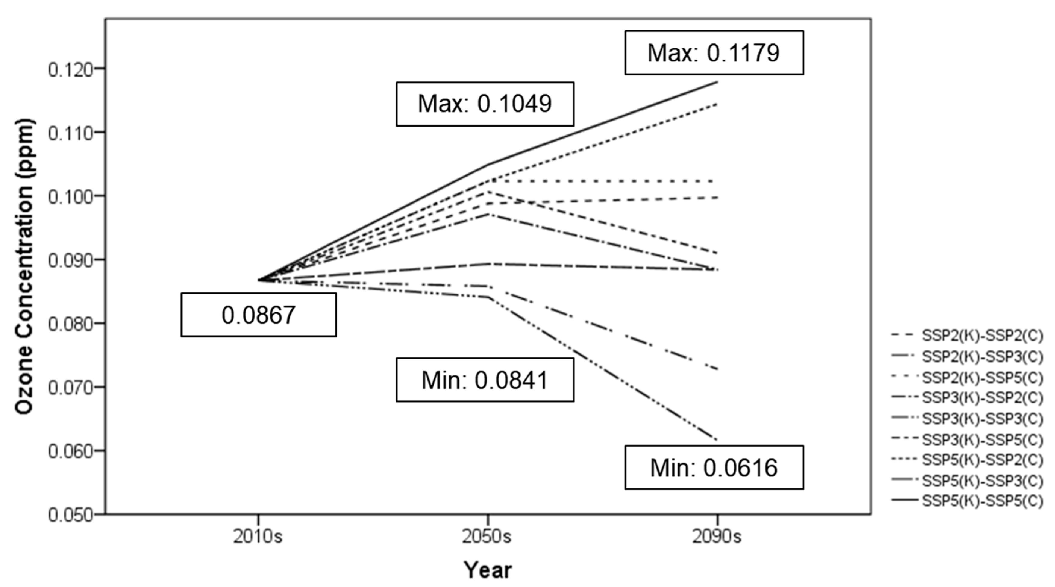
The Carnegie Ames Stanford Approach (CASA)-NPP values used in the model were developed using the 10-year average of 592.53 tC/km2/year (SD: 213.72 tC/km2/year); over the last decade the ozone concentration in the forest areas in the second and third quarters had a mean of 0.0867 ppm (SD 0.0395 ppm).
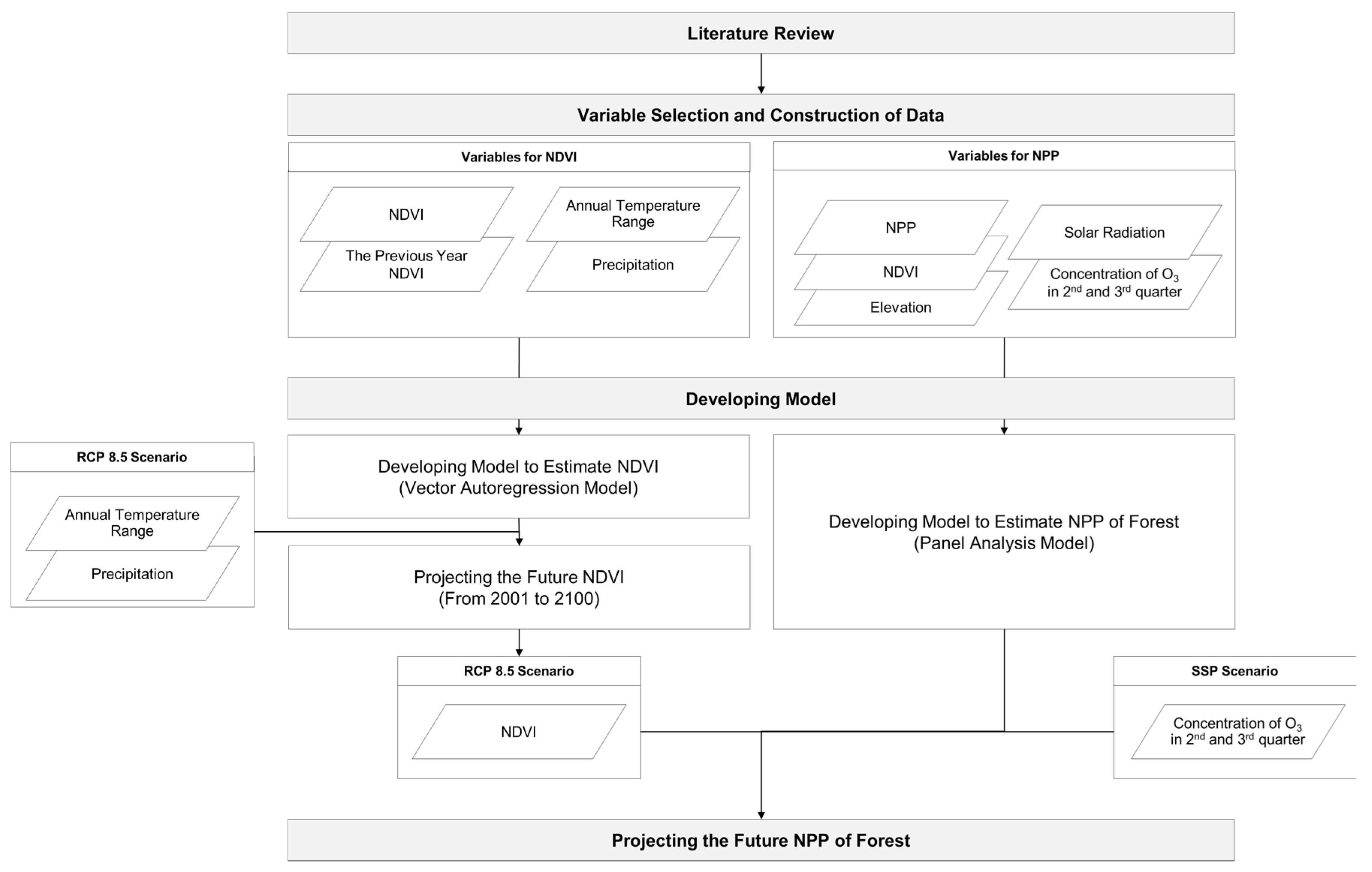
First, we estimated the future NDVI using a vector autoregressive model to reflect changes in vegetation over time, such as future forest distribution. The NDVI estimation model was developed using variables that affect vegetation activity. The independent variables used in the NDVI estimation model are the previous year’s NDVI, annual precipitation, and annual temperature range (Table 2). The higher the NDVI value in the previous year, the higher the NDVI value in the year being observed. Higher annual precipitation and a higher annual temperature range lead to a higher NDVI value.
Second, we estimated the future NPP using a panel analysis model to reflect the ozone concentration. This is the result of panel analysis model selection before the panel analysis result. A one-way time and random effect model was selected as the most suitable panel analysis model among the various panel analysis models considered in this study. Specifically, we selected the time effect model of the one-way model through the Least Square Dummy Variable (R-sq.: 0.9746) and Chow-test (F-value: 70.63, Sig.: 0.000). Next, we determined that random effects model is more significant through the Breusch and Pagan Lagrangian Multiplier test (see Table A2) and the Hausman test (see Table A3). The Breusch and Pagan Lagrangian Multiplier test results showed that both of the models were significant, but the random effect model was chosen because the null hypothesis, where the difference in coefficients was not systematic, could not be rejected by Hausman test. Finally, one-way time and random effects models were selected by this process. Also, the rho value in context of the random effect model indicates the estimated proportion of the between variance at the total variance was about 0.86. In addition, the Durbin-Watson test value was 1.722, indicating that there was no time-series autocorrelation between each variable.
The independent variables used to develop the net primary productivity of the forest impact model when considering the effects of ozone are NDVI, solar radiation, altitude, and average concentration of ozone in the second and third quarters.
According to the results, NPP tends to increase, and NPP increases with increasing NDVI and solar radiation. However, as the altitude increased, NPP decreased, as shown in Table 3. The concentration of ozone has a negative effect on NPP. The analysis suggests that the ozone concentration begin exerting effects to the NPP, about 68.10 tC/km2/year decrement per 0.01 ppm increment. NDVI and previous year NDVI, annual precipitation, annual temperature range, solar radiation, altitude, and average ozone concentrations in the second and third quarters were found to have an impact on vegetation growth. The NPP estimation model, which reflects the effects of ozone, is shown in Table 3.
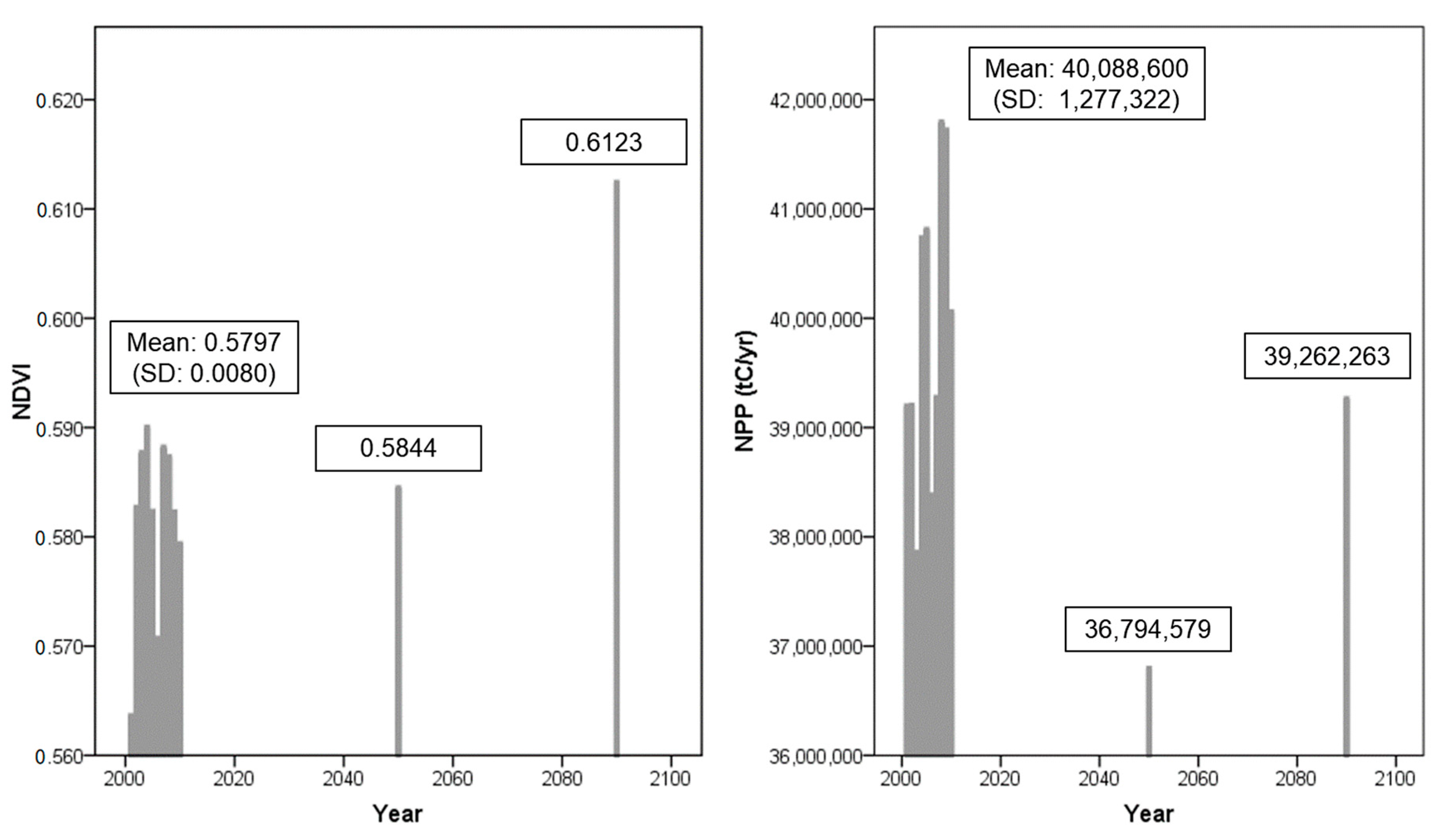
The NDVI and the net primary productivity of forests estimates derived from the results are shown in Figure 3. Figure 3 shows the annual mean value of NDVI, the net primary productivity of forests used as input data, and the 10-year mean value in the future. The values of NDVI were about 0.58~0.61 and were within the range of the NDVI value of forest [74]. The values of NDVI in this study are similar to the values that are found in other studies [75]. The net primary productivity of forests for the last decade was about 630–696 tC/km2/year, and the average NPP for the last 10 years was about 663 tC/km2/year (SD: 21 tC/km2/year). The average value of the total NPP of Korea is about 40 million tC/year. The year 2003 had the lowest NPP, at about 38 million tC/year, and the highest NPP value was about 42 million tC/year in 2009. The independent variables in 2003 showed that precipitation, NDVI, and temperature range were higher than in other years, but solar radiation was notably low. The low productivity in 2003 was due to this comparatively lower solar radiation. In addition, the NPP of forests was the highest in 2009 because of that year’s comparatively higher amount of solar radiation; precipitation and NDVI values were similar to those of other years, but the highest level of radiation was observed in 2009. Based on all of the available information, we concluded that the distribution of these input variables affected the results. Furthermore, both NPP and NDVI are expected to decrease in the 2050s, when compared to their current levels, and they are expected to increase in the 2090s compared to their 2050s levels. However, NDVI increases compared to its present level in the 2090s, but NPP is expected to decrease compared to its current level during the same period. This implies that NDVI estimation is related to variables such as temperature and precipitation, but it can be assumed that the change in ozone concentration influenced NPP estimation. However, the empirical model has a disadvantage in that it can be only applied to the region for model developing [76], and there is a limitation that the actual technology is reflected [41,77].

3.2. Relationships among Climate Change, Ozone Concentration and the Net Primary Productivity of Forest

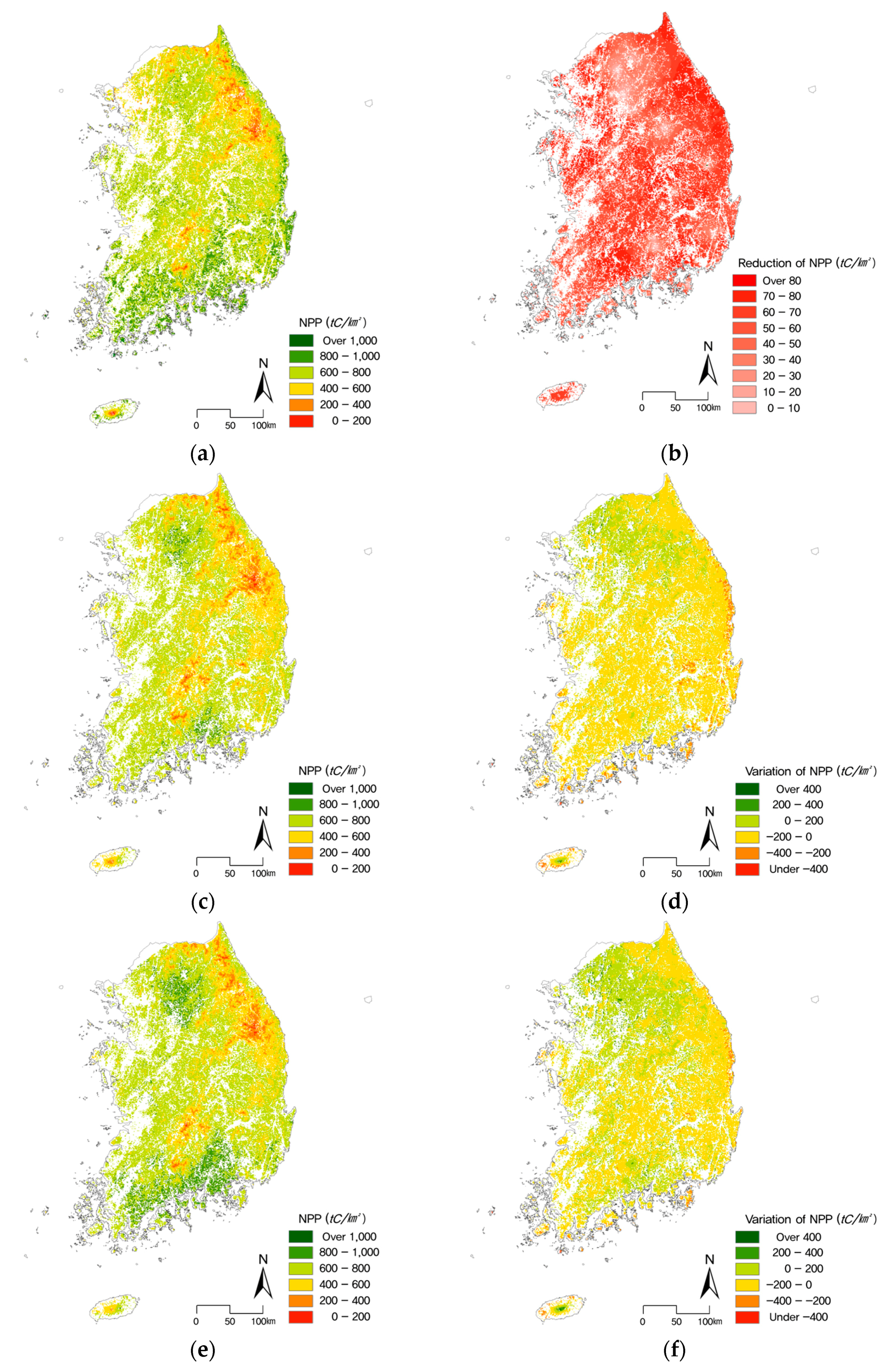
Figure 4 shows the differences and spatial distributions of the net primary productivity of forests with the effects of ozone at present and its variation due to ozone concentration and climate change. In Figure 4, the net primary productivity of forests in the southern region is higher than that of the central region due to variables, such as temperature range, precipitation, and solar radiation, and the forest productivity in the central inland region is relatively higher than in the rest of the central region. This is because solar radiation and temperature have an influence on the distribution of the net primary productivity of forests [78]; the forest region has a lower amount of solar radiation and lower temperatures than the central inland region, which is why it has a lower NPP than the inland region [79]. Another study showed that carbon from 585 tC/km2/year, to 731 tC/km2/year is stored in vegetation every year, which is similar to the results of this study [80].
Also, using the point data in the results, we examined the differences between forest type and region; the Kruskal-Wallis test was used to do this. The results showed that the net primary productivity of forests, NDVI, and ozone concentrations differed significantly by region. However, there was no difference between the two groups when they were classified using the same method. This is because the differences between forest types were reflected in the process of deriving the future variables of NDVI.
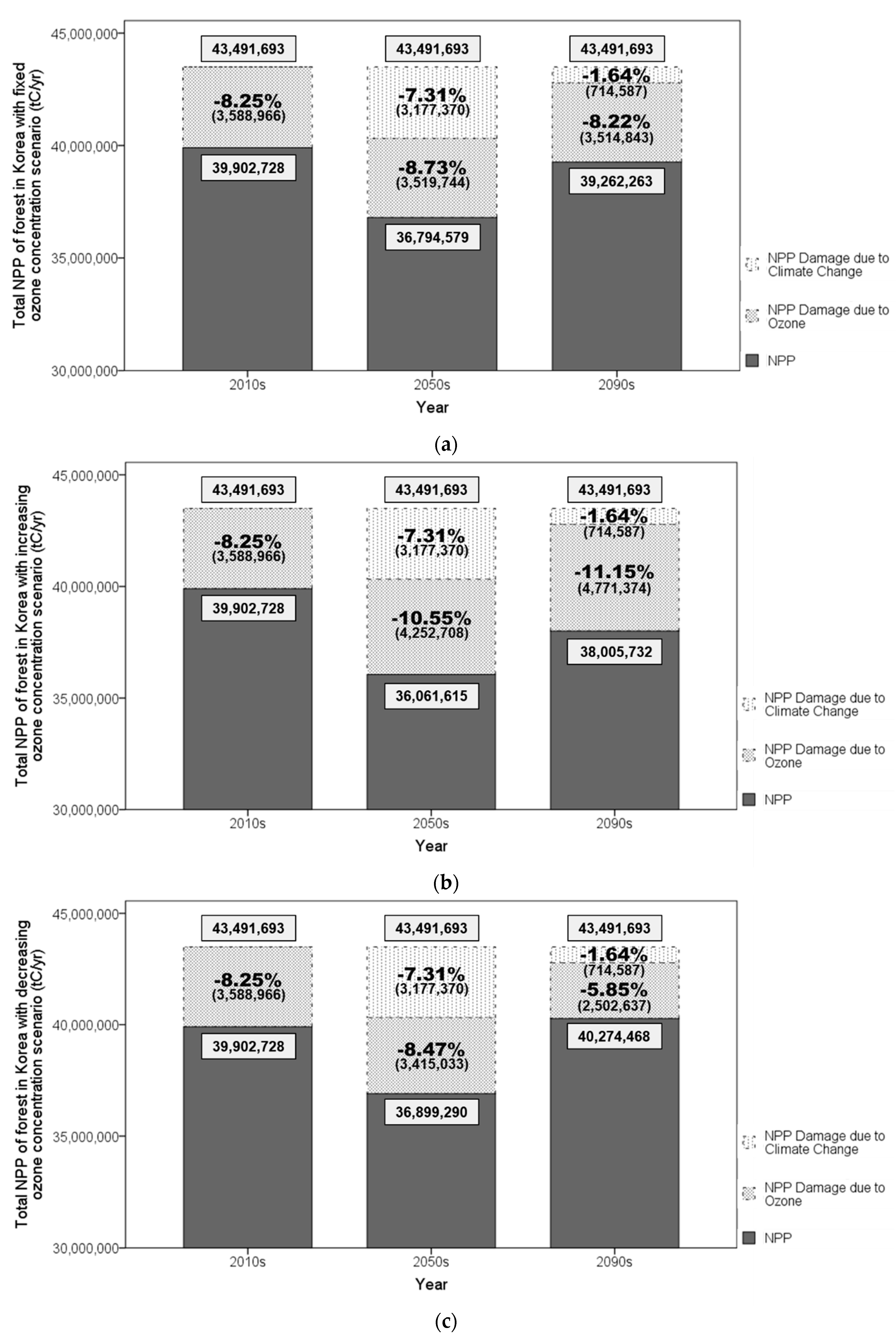
Figure 5 shows the result of the model derived in this study, which estimates the net primary productivity of forests when ozone concentration maintains its current level, when it increases to its maximum potential level, and when it decreases to its absolute lowest potential level. The current average net primary productivity of forests is about 40 million tC/year, which is about 36 million to 37 million tC/eayr in the 2050s and 38 million to 40 million tC/year in the 2090s. The net primary productivity of forests is expected to increase in the 2090s when compared to the net primary productivity in the 2050s due to an increase in temperature and precipitation. The results of this study show that adaptation policies are important for managing forest productivity in response to climate change. We can consider that adaptation policies may be more useful in forest policy because of the potential for increasing the net primary productivity of forests in future climate change scenarios because some variables will affect forest growth.
The damage that is caused by ozone to the net primary productivity of forests was as high as 27.07% in individual analysis units, with the average amount of damage when all the analysis units were analyzed measuring 9.08%. The total net primary productivity of forests in Korea was estimated to be about 43 million tC/year without the effects of ozone and about 40 million tC/year considering the ongoing effects of ozone accounting for the 10-year average. From 2001 to 2010, the NPP of forests decreased due to ozone by an average of about 8.25% in Korea. According to a study by Ollinger et al. [43], the decrease in forest productivity due to ozone in the United States has decreased by at least 3% to 16%, an average of 7.4%, in 64 sites from 1987 to 1992, and Felzer et al. [19] found that annual forest productivity decreased from 1987 to 1992 by 2.6 ± 0.34%. In particular, the average concentration of ozone during the second and third quarters, when NPP is in full swing, has the greatest impact. According to these studies that ozone influences NPP production at a mean concentration of 0.04 ppm or higher [19,43]. In fact, the concentration observed was about 0.05 ppm, indicating a concentration that influences NPP production. Damage also is expressed when contact is made between 0.06 ppm and 0.170 ppm for 4 h and between 0.200 ppm and 0.510 ppm for 1 h for susceptible species [7]. In general, it is also known that after 20 days of exposure, yield is reduced by 50% in the case of radish at 0.05 ppm per 1 day, and carnations are affected by a decrease in flowering rate and a decrease in the production of pollen.
In the future, ozone concentration changes due to nitrogen oxide emissions from various scenario combinations are expected to decrease by up to between 3% and 21% when compared to current levels in the 2050s and between 29% or 36% in the 2090s (see Figure 2 in Section 2.2.3). Changes in the net primary productivity of forests due to ozone concentration change scenarios are shown in Figure 5. When average ozone concentration decreases by about 3% in the 2050s, the net primary productivity of forests increases by about 0.28%. When the average ozone concentration increases by about 21%, the productivity of the net primary productivity of forests decreases by about 1.99%. In the 2090s, when the average ozone concentration decreases by about 29%, the net primary productivity of forests increases by 2.58%, and when the ozone concentration increases by about 36%, the net primary productivity decreases by about 3.20%. Under the RCP 8.5 scenario, an increase in ozone and its impact on vegetation is simulated in Asia, where a strong decrease in NPP (1.0–1.5% per year) was simulated [15,81,82]. A reduction of the ozone impact on vegetation is observed in particular over the Eastern US and in Southeastern China by 2100 [15]. A study evaluated the effects of tropospheric ozone on GPP at 37 European forest sites during the time period 2000–2010 and showed, along a North-West/South-East European transect, a negative impact of ozone on GPP, ranging from 0.4% to 30% [83].
The results obtained from predicting the damage caused by ozone are different from the results of the impact assessment of climate change. The net primary productivity of forests due to climate change may increase with management or adaptation policies, but damage from ozone results in a decrease in productivity as the concentration of ozone increases. These results show that mitigation policies are important to reduce the negative impact of ozone on net primary productivity of forests. Reducing nitrogen oxide emissions and decreasing the concentration of ozone generated, thereby will also reduce the damage to forest productivity.

4. Conclusions

This study investigated the relationship between ozone concentration in the second and third quarters and the net primary productivity of forest and estimated the damage that is caused by ozone when the ozone concentration was fixed and when it changed. Three phase analyses were conducted; (1) an empirical model was developed that can represent the current net primary productivity of forests, reflecting the concentration of ozone; (2) the relationship between ozone concentration and the current net primary productivity of forests was analyzed by using cross-section time series analysis; and (3) estimates of future net primary productivity of forests and the impact of future ozone concentrations on forest fertility were made using the future ozone concentration data estimated using the temperature and precipitation data of the RCP 8.5 scenario and the NOx emissions of the SSP scenarios.
According to the results of this study, the net primary productivity of forests was reduced by 8.25% due to ozone levels at present, and the damage to NPP is estimated to be between 8.47% to 10.55% in the 2050s and 5.85% to 11.15% in the 2090s. Climate change will negatively affect the net primary productivity by an estimated 7.31% in the 2050s and 1.64% in the 2090s. The relationship between carbon dioxide at current or future levels and the productivity of plants is controversial, but the negative relationship between ozone concentration and the net primary productivity of forests is clear, as indicated by the results of this study.
The significance of this study is that the effect of ozone on the net primary productivity was statistically figured out in macro scale. Also, the estimation of the net primary productivity of forests in the future is reflected not only in the climate data, but also in the concentration of ozone based on emissions in SSP scenarios to calculate future ozone concentrations, rather than to make assumptions based on a simply scenario. This is another significance of this study, as compared to other studies that can estimate the damage due to the changes of carbon dioxide concentration. These findings of this study offer policy implications on climate change mitigation and adaptation or international environmental negotiations. However, in future studies it will be necessary to apply methods which overcome the limitation of the empirical model, as well as to find a method to increase the accuracy of the model.
In many studies, it is suggested that future ozone concentration is likely to increase due to climate change. This means that future damage to forests due to ozone is expected to increase beyond the current level of damage. Therefore, we consider that the effect of ozone is no longer a problem only in Korea, but rather a problem facing all of East Asia, including China and Japan, and that it also be viewed as a global problem. For more accurate forecasting, cooperation among domestic and international researchers will be needed.

Acknowledgments

This work was supported by grants from the National Institute of Environment Research (NIER-2015-02-02-040) and the Public Technology Program based on Environmental Policy (Project No. 2016000210004), which are funded by the Ministry of Environment of Republic of Korea.

Author Contributions

All authors have contributed to the intellectual content of this paper. Jin Han Park designed this study and analyzed the data and wrote the manuscript. Chan Park, Songyi Kim, Sunyong Sung and Sung Chul Hong contributed to make the data and to analyze. Dong Kun Lee, Jianbang Gan and Tae Yong Jung provided some core advice and checked through the paper’s entirety.

Conflicts of Interest

The authors declare no conflict of interest.

Appendix A

Variables selected by literature review, correlation analysis, and expert interview.
First, we collected variables which are related to photosynthesis through a literature review. Mean temperature, maximum temperature, minimum temperature, the highest temperature of the warmest month, the lowest temperature of the coldest month, annual temperature range, precipitation and its related variables, and solar radiation were selected as the climate variables. Slope, elevation and aspect were selected as the topographical variables. Leaf Area Index (LAI), Normal Distribution Vegetation Index (NDVI), evapotranspiration and potential evapotranspiration were chosen as variables related to the plants.
Next, we selected primary variables through correlation analysis (Table A1). When we use all variables which have significance, the results have a probability of multicollinearity. Thus, we needed to focus on more significant variables. As a result, we selected mean temperature, annual temperature range, precipitation, solar radiation, elevation, slope, ozone concentration in 2nd and 3rd quarters, DVI, and previous year NDVI.
Third, we conducted two interviews with experts who work in the field of forest ecophysiology on the variables selected by correlation analysis. According to their comments, mean temperature might overlap with annual temperature range. In addition, slope might also overlap with elevation. It was also said that elevation will have an effect on forest growth than slope because of the relationship between elevation and temperature.
Finally, we selected annual temperature range, precipitation, NDVI and the previous year’s NDVI to develop a model to predict future NDVI. Furthermore, solar radiation, elevation, NDVI and the concentration of ozone in the 2nd and 3rd quarters were selected as variables for developing a model to estimate future NPP.
Table A1. Results of correlation analysis.
CategoriesVariablesNPP
Pearson CorrelationSig. (2-Tailed)n
Plants variableNDVI0.641 **0.000630
Previous year NDVI0.604 **0.000567
Evapotranspiration0.162 **0.000630
Potential evapotranspiration0.155 **0.000630
Climate variableMean temperature0.169 **0.000630
Maximum temperature0.240 **0.000630
Minimum temperature0.170 **0.000630
The highest temperature of the warmest month−0.0230.561630
The lowest temperature of the coldest month0.273 **0.000630
Annual temperature range−0.280 **0.000630
Precipitation0.141 **0.000630
Solar radiation0.295 **0.000630
Topographical variableAspectc630
Elevation0.099 *0.013630
Slope0.258 **0.000630
Air pollutant variableOzone concentration in 2nd and 3rd quarters−0.282 **0.000630
Annual average of ozone concentration−0.131 **0.002630
**: Correlation is significant at the 0.01 level (2-tailed); *: Correlation is significant at the 0.05 level (2-tailed); c: Cannot be computed because at least one of the variables is constant.

Appendix B

The results of the specification test used to select the panel analysis model in this study are shown in the Table A2 and Table A3 below.
Table A2. Results of the Breusch-Pagan LM test.
VarSd = Sqrt(Var)
NPP4,567,9522137.277
e277,079.1526.383
u1,757,3451325.649
Test: Var(u) = 0; chi2(1) = 2030.07; Prob > chi2 = 0.0000.
Table A3. Results of the Hausman test.
(b) id_fe(B) id_re(b-B) DifferenceSqrt (diag(V_b-V_B)) S.E.
O3 Con. *−5250.073−6810.4161560.3434354.144
NDVI1.1768511.1746440.00220690.0291254
Solar radiation1.0364751.051382−0.01490710.0097422
* O3 Con.: Average concentration of ozone in 2nd and 3rd quarters; b = consistent under Ho and Ha; obtained from xtreg; B = inconsistent under Ha, efficient under Ho; obtained from xtreg; Test: Ho: difference in coefficients not systematic; chi2(2) = (b-B)’[(V_b-V_B)^(-1)](b-B)= 0.13; Prob > chi2 = 0.7201; (V_b-V_B is not positive definite).

References

  1. Costanza, R.; D’Arge, R.; De Groot, R.; Farber, S.; Grasso, M.; Hannon, B.; Limburg, K.; Naeem, S.; O’Neill, R.V.; Paruelo, J.; et al. The value of the world’s ecosystem services and natural capital. Nature 1997, 387, 253–260. [Google Scholar] [CrossRef]
  2. Daily, G.C. Nature’s Services; Island Press: Washington, DC, USA, 1997. [Google Scholar]
  3. Millennium Ecosystem Assessment. Ecosystems and Human Well-Being; Island Press: Washington, DC, USA, 2003. [Google Scholar]
  4. De Groot, R.S.; Wilson, M.A.; Boumans, R.M.J. A typology for the classification, description and valuation of ecosystem functions, goods and services. Ecol. Econ. 2002, 41, 393–408. [Google Scholar] [CrossRef]
  5. Johnson, D.W.; Turner, J.; Kelly, J.M. The Effects of Acid Rain on Forest Nutrient Status. Water Resour. Res. 1982, 18, 449–461. [Google Scholar] [CrossRef]
  6. Likens, G.E.; Bormann, F.H. Acid Rain: A Serious Regional Environmental Problem. Science 1974, 184, 1176–1179. [Google Scholar] [CrossRef] [PubMed]
  7. Lee, S.; Byun, J.; Chae, K.; Jeong, J.; Sung, J.; Kwon, T.; Cho, J.; Kim, Y.; Lee, C. Air Pollution and Forest Ecosystem Change; Korea Forest Research Institute: Seoul, Korea, 2011. [Google Scholar]
  8. Fuhrer, J.; Skarby, L.; Ashmore, M.R. Critical levels for ozone effects on vegetation in Europe. Environ. Pollut. 1997, 97, 91–106. [Google Scholar] [CrossRef]
  9. Bytnerowicz, A.; Omasa, K.; Paoletti, E. Integrated effects of air pollution and climate change on forests: A northern hemisphere perspective. Environ. Pollut. 2007, 147, 438–445. [Google Scholar] [CrossRef] [PubMed]
  10. Nowak, D.J.; Hoehn III, R. E.; Crane, D.E.; Stevens, J.C.; Walton, J.T. Assessing Urban Forest Effects and Values; United States Department of Agriculture: Washington, DC, USA, 2007. [Google Scholar]
  11. World Meteorological Organization; Global Ozone Research; Monitoring Project. Atmospheric Ozone 1985: Assessment of Our Understanding of the Processes Controlling Its Present Distribution and Change; National Aeronautics and Space Administration: Washington, DC, USA, 1985. [Google Scholar]
  12. Chameides, W.; Walker, J.C.C.G. A photochemical theory of tropospheric ozone. J. Gecophys. Res. 1973, 78, 8751–8760. [Google Scholar] [CrossRef]
  13. Logan, J.A.; Prather, M.J.; Wofsy, S.C.; Mcelroy, M.B. Tropospheric chemistry: A global perspective. J. Geophys. Res. 1981, 86, 7210–7254. [Google Scholar] [CrossRef]
  14. National Research Council. Ozone-Forming Potential of Reformulated Gasoline; National Academies Press: Washington, DC, USA, 1999; ISBN 978-0-309-06445-3. [Google Scholar]
  15. Sicard, P.; Anav, A.; De Marco, A.; Paoletti, E. Projected global ground-level ozone impacts on vegetation under different emission and climate scenarios. Atmos. Chem. Phys. 2017, 17, 12177–12196. [Google Scholar] [CrossRef]
  16. Sitch, S.; Cox, P.M.; Collins, W.J.; Huntingford, C. Indirect radiative forcing of climate change through ozone effects on the land-carbon sink. Nature 2007, 448, 791–794. [Google Scholar] [CrossRef] [PubMed]
  17. Han, S.; Lee, J.; Lee, G.; Oh, C. Ozone Tolerance Mechanism and Damage Symptoms of Forests; Korea Forest Research Institute: Seoul, Korea, 2006. [Google Scholar]
  18. Ainsworth, E.A.; Yendrek, C.R.; Sitch, S.; Collins, W.J.; Emberson, L.D. The effects of tropospheric ozone on net primary productivity and implications for climate change. Annu. Rev. Plant Biol. 2012, 63, 637–661. [Google Scholar] [CrossRef] [PubMed]
  19. Felzer, B.; Kicklighter, D.; Melillo, J.; Wang, C.; Zhuang, Q.; Prinn, R. Effects of ozone on net primary production and carbon sequestration in the conterminous United States using a biogeochemistry model. Tellus B 2004, 56, 230–248. [Google Scholar] [CrossRef]
  20. Krupa, S.V.; Manning, W.J. Atmospheric ozone: Formation and effects on vegetation. Environ. Pollut. 1988, 50, 101–137. [Google Scholar] [CrossRef]
  21. Lindroth, R.L.; Kopper, B.J.; Parsons, W.F.J.; Bockheim, J.G.; Karnosky, D.F.; Hendrey, G.R.; Pregitzer, K.S.; Isebrands, J.G.; Sober, J. Consequences of elevated carbon dioxide and ozone for foliar chemical composition and dynamics in trembling aspen (Populus tremuloides) and paper birch (Betula papyrifera). Environ. Pollut. 2001, 115, 395–404. [Google Scholar] [CrossRef]
  22. Noormets, A.; Sober, A.; Pell, E.J.; Dickson, R.E.; Podila, G.K.; Sober, J.; Isebrands, J.G.; Karnosky, D.F. Stomatal and non-stomatal limitation to photosynthesis in two trembling aspen (Populus tremuloides Michx.) clones exposed to elevated CO2 and/or O3. Plant Cell Environ. 2001, 24, 327–336. [Google Scholar] [CrossRef]
  23. D’Amato, G.; Cecchi, L. Effects of climate change on environmental factors in respiratory allergic diseases. Clin. Exp. Allergy 2008, 38, 1264–1274. [Google Scholar] [CrossRef] [PubMed]
  24. Jang, A.-S. Climate change and air pollution. J. Korean Med. Assoc. 2011, 54, 175. [Google Scholar] [CrossRef]
  25. Bernard, S.M.; Samet, J.M.; Grambsch, A.; Ebi, K.L.; Romieu, I. The potential impacts of climate variability and change on air pollution-related health effects in the United States. Environ. Health Perspect. 2001, 109 (Suppl. 2), 199–209. [Google Scholar] [CrossRef] [PubMed]
  26. Chen, K.-S.; Ho, Y.T.; Lai, C.H.; Tsai, Y.A.; Chen, S.-J. Trends in concentration of ground-level ozone and meteorological conditions during high ozone episodes in the Kao-Ping Airshed, Taiwan. J. Air Waste Manag. Assoc. 2004, 54, 36–48. [Google Scholar] [CrossRef] [PubMed]
  27. Grambsch, A. Climate change and air quality. Potential Impacts Clim. Chang. Transp. 2004, 23, 39–42. [Google Scholar]
  28. Prather, M.; Gauss, M.; Berntsen, T.; Isaksen, I.; Sundet, J.; Bey, I.; Brasseur, G.; Dentener, F.; Derwent, R.; Stevenson, D.; et al. Fresh air in the 21st century? Geophys. Res. Lett. 2003, 30, 2–5. [Google Scholar] [CrossRef]
  29. Zhang, M.; Xu, Y.; Itsushi, U.; Hajime, A. A numerical study of tropospheric ozone in the springtime in East Asia. Adv. Atmos. Sci. 2004, 21, 163–170. [Google Scholar] [CrossRef]
  30. Grygalashvyly, M.; Sonnemann, G.R.; Lübken, F.; Hartogh, P.; Berger, U.; Sonnemann, G.R.; Lübken, F.; Hartogh, P.; Berger, U. Transport of NOx in East Asia identified by satellite and in situ measurements and Lagrangian particle dispersion model simulations. J. Geophys. Res. Atmos. 2014, 1–29. [Google Scholar] [CrossRef]
  31. Li, J.; Yang, W.; Wang, Z.; Chen, H.; Hu, B.; Li, J.; Sun, Y.; Fu, P.; Zhang, Y. Modeling study of surface ozone source-receptor relationships in East Asia. Atmos. Res. 2016, 167, 77–88. [Google Scholar] [CrossRef]
  32. Choi, K.-C.; Lee, J.-J.; Bae, C.H.; Kim, C.-H.; Kim, S.; Chang, L.-S.; Ban, S.-J.; Lee, S.-J.; Kim, J.; Woo, J.-H. Assessment of transboundary ozone contribution toward South Korea using multiple source–receptor modeling techniques. Atmos. Environ. 2014, 92, 118–129. [Google Scholar] [CrossRef]
  33. Sim, C.S.; Seo, J.H. Air Quality Issues Associated with Future Domestic Coal Power Planning and Emission Projections of East Asia; Korea Environment Institute: Sejong, Korea, 2013. [Google Scholar]
  34. Nagashima, T.; Ohara, T.; Sudo, K.; Akimoto, H. The relative importance of various source regions on East Asian surface ozone. Atmos. Chem. Phys. 2010, 10, 11305–11322. [Google Scholar] [CrossRef]
  35. Kaitala, V.; Pohjola, M.; Tahvonen, O. Transboundary air pollution and soil acidification: A dynamic analysis of an acid rain game between Finland and the USSR. Environ. Resour. Econ. 1992, 2, 161–181. [Google Scholar] [CrossRef]
  36. Lam, K.S.; Wang, T.J.; Wu, C.L.; Li, Y.S. Study on an ozone episode in hot season in Hong Kong and transboundary air pollution over Pearl River Delta region of China. Atmos. Environ. 2005, 39, 1967–1977. [Google Scholar] [CrossRef]
  37. Dong, J.-I. Ambient Air Quality of China and Transboundary Transport of Air Pollutants. Korean J. Sanit. 1993, 8, 49–66. [Google Scholar]
  38. Gibbs, H.K.; Brown, S.; Niles, J.O.; Foley, J.A. Monitoring and estimating tropical forest carbon stocks: Making REDD a reality. Environ. Res. Lett. 2007, 2, 45023. [Google Scholar] [CrossRef]
  39. Adams, B.; White, A.; Lenton, T.M. An analysis of some diverse approaches to modelling terrestrial net primary productivity. Ecol. Modell. 2004, 177, 353–391. [Google Scholar] [CrossRef]
  40. Michaletz, S.T.; Cheng, D.; Kerkhoff, A.J.; Enquist, B.J. Convergence of terrestrial plant production across global climate gradients. Nature 2014, 512, 39–43. [Google Scholar] [CrossRef] [PubMed]
  41. Na, S., II; Hong, S.Y.; Kim, Y.H.; Lee, K.D.; Jang, S.Y. Prediction of Rice Yield in Korea using Paddy Rice NPP index-Application of MODIS data and CASA Model. Korean J. Remote Sens. 2013, 29, 461–476. [Google Scholar] [CrossRef]
  42. Ito, A. The regional carbon budget of East Asia simulated with a terrestrial ecosystem model and validated using AsiaFlux data. Agric. For. Meteorol. 2008, 148, 738–747. [Google Scholar] [CrossRef]
  43. Ollinger, S.V.; Aber, J.D.; Reich, P.B. Simulating ozone effects on forest productivity: Interactions among leaf-, canopy-, and stand-level processes. Ecol. Appl. 1997, 7, 1237–1251. [Google Scholar] [CrossRef]
  44. Running, S.W.; Zhao, M. User’s Guide Daily GPP and Annual NPP (MOD17A2/A3) Products NASA Earth Observing System MODIS Land Algorithm; NASA Press: Washington, DC, USA, 2015. [Google Scholar]
  45. Tol, R.S.J.; Fankhauser, S.; Richels, R.G.; Smith, J.B. How much damage will climate change do? Recent estimates. World Econ. Thames 2000, 1, 179–206. [Google Scholar]
  46. Yuan, J.; Niu, Z.; Wang, C. Vegetation NPP distribution based on MODIS data and CASA model—A case study of northern Hebei Province. Chinese Geogr. Sci. 2006, 16, 334–341. [Google Scholar] [CrossRef]
  47. Potter, C.; Klooster, S.; Myneni, R.; Genovese, V.; Tan, P.N.; Kumar, V. Continental-scale comparisons of terrestrial carbon sinks estimated from satellite data and ecosystem modeling 1982–1998. Glob. Planet. Chang. 2003, 39, 201–213. [Google Scholar] [CrossRef]
  48. Yu, Y.; Chen, J.M.; Yang, X.; Fan, W.; Li, M.; He, L. Influence of site index on the relationship between forest net primary productivity and stand age. PLoS ONE 2017, 12, 1–20. [Google Scholar] [CrossRef] [PubMed]
  49. Turner, D.P.; Cohen, W.B.; Kennedy, R.E.; Fassnacht, K.S.; Briggs, J.M. Relationships between leaf area index and Landsat TM spectral vegetation indices across three temperate zone sites. Remote Sens. Environ. 1999, 70, 52–68. [Google Scholar] [CrossRef]
  50. Wang, Q.; Adiku, S.; Tenhunen, J.; Granier, A. On the relationship of NDVI with leaf area index in a deciduous forest site. Remote Sens. Environ. 2005, 94, 244–255. [Google Scholar] [CrossRef]
  51. Fan, L.; Gao, Y.; Brück, H.; Bernhofer, C. Investigating the relationship between NDVI and LAI in semi-arid grassland in Inner Mongolia using in-situ measurements. Theor. Appl. Climatol. 2009, 95, 151–156. [Google Scholar] [CrossRef]
  52. Johnson, L.F. Temporal stability of an NDVI-LAI relationship in a Napa Valley vineyard. Aust. J. Grape Wine Res. 2003, 9, 96–101. [Google Scholar] [CrossRef]
  53. Goswami, S.; Gamon, J.; Vargas, S.; Tweedie, C. Relationships of NDVI, Biomass, and Leaf Area Index (LAI) for Six Key Plant Species in Barrow, Alaska; ProQuest Press: Ann Arbor, MI, USA, 2015. [Google Scholar]
  54. Lee, K. Change of Forest Ecosystem because of Air Pollution and Acid Rain. Envirion. Symp. Air Quility Manag. Busan 1996, 1996, 26–40. [Google Scholar]
  55. Woo, S.-Y.; Lee, S.H.; Kwan, K.W.; Lee, J.C.; Choi, J.H. Growth, Photosynthesis, and Ascorbate Peroxidase Activity of Several Species to the Ozone Exposure. J. Korean For. Soc. 2004, 93, 409–414. [Google Scholar]
  56. Lee, K.J.; Han, S.H.; Kim, G.B.; Kim, T.K. A study on the Correlation between Ambient Ozone Concentration and Tree Health of Zelkova serrata Makino Street Trees In Seoul. Bull. Arbor. SEOUL Natl. Univ. 1999, 19, 54–65. (In Korean) [Google Scholar]
  57. Reig-Armiñana, J.; Calatayud, V.; Cerveró, J.; Garcıa-Breijo, F.J.; Ibars, A.; Sanz, M.J. Effects of ozone on the foliar histology of the mastic plant (Pistacia lentiscus L.). Environ. Pollut. 2004, 132, 321–331. [Google Scholar] [CrossRef] [PubMed]
  58. Singh, H.B.; Ludwig, F.L.; Johnson, W.B. Tropospheric ozone: Concentrations and variabilities in clean remote atmospheres. Atmos. Environ. 1978, 12, 2185–2196. [Google Scholar] [CrossRef]
  59. Logan, J.A. Ozone in rural areas of the United States. J. Geophys. Res. Atmos. 1989, 94, 8511–8532. [Google Scholar] [CrossRef]
  60. Han, C. Lecture for Panel Data; PAKYOUNGSA: Seoul, Korea, 2017. [Google Scholar]
  61. Min, I.; Choi, P. STATA Panel Data Analysis; The Korean Association of STATA: Seoul, Korea, 2009. [Google Scholar]
  62. Lee, H.; No, S. Advanced Statistical Analysis; Moonwoosa: Goyang, Korea, 2012. [Google Scholar]
  63. Moon, G. Vector Autoregressive Model: VAR. J. Korean Off. Stat. 1997, 2, 23–56. [Google Scholar]
  64. Stock, J.H.; Watson, M.W.; Stock, J.H.; Watson, M.W. Vector Autoregressions. J. Econ. Perspect. 2001, 15, 101–115. [Google Scholar] [CrossRef]
  65. New, M.; Hulme, M.; Jones, P. Representing twentieth-century space-time climate variability. Part II: Development of 1901–1996 monthly grids of terrestrial surface climate. J. Clim. 2000, 13, 2217–2238. [Google Scholar] [CrossRef]
  66. Abrigo, M.R.M.; Love, I. Estimation of panel vector autoregression in Stata. Stata J. 2016, 16, 778–804. [Google Scholar] [CrossRef]
  67. Bierens, H.J. VAR Models with Exogenous Variables. Available online: http://www.personal.psu.edu/hxb11 /EasyRegTours/VAR_Tourfiles/VARX.PDF (accessed on 16 June 2017).
  68. Marquez, J.; Spanos, A.; Adams, F.G.; Balestra, P.; Dagenais, M.G.; Kendrick, D.; Pindyck, R.S.; Welfe, W. The Econometrics of Panel Data; Springer: Beilin, Germany, 2008; ISBN 9783540689201. [Google Scholar]
  69. Edwards, J.A. Building Better Econometric Models Using Cross Section and Panel Data; Business Expert Press: New York, NY, USA, 2014. [Google Scholar]
  70. Raj, B.; Baltagi, B.H. Panel Data Analysis; Springer Science & Business Media: Beilin, Germany, 2012; ISBN 9783642501296. [Google Scholar]
  71. Lee, C.; Kim, S.; Kim, J.-C. Detailed Investigation to Identify the Cuase of High Concentration of Ozone Generation (III); National Institute of Environmental Research: Incheon, Korea, 2011. [Google Scholar]
  72. Shin, H.; Son, J.; Roh, S.; Park, J.; Lee, M.; Kim, J. The Study on the Meteorology Adjusted Long Term Trend of Ozone Induced by the Statistical Model; National Institute of Environmental Research: Incheon, Korea, 2012. [Google Scholar]
  73. Park, J.H.; Lee, D.-K.; Lee, M.-J.; Park, C.; Jung, T.-Y.; Kim, S.-K.; Hong, S.-C.; Baek, S.-J.; Lee, J.-H. Estimating Climate Pollutants Emissions and Service Demands considering Socio-economic Change: Residential·Commercial Sector, Transportation Sector, Industrial Sector. J. Clim. Chang. Res. 2015, 6, 291. [Google Scholar] [CrossRef]
  74. Lunetta, R.S.; Knight, J.F.; Ediriwickrema, J.; Lyon, J.G.; Worthy, L.D. Land-cover change detection using multi-temporal MODIS NDVI data. Remote Sens. Environ. 2006, 105, 142–154. [Google Scholar] [CrossRef]
  75. Jin, Y.; Sung, S.; Lee, D.K.; Biging, G.S.; Jeong, S. Mapping deforestation in north korea using phenology-based multi-index and random forest. Remote Sens. 2016, 8, 997. [Google Scholar] [CrossRef]
  76. Becker-Reshef, I.; Vermote, E.; Lindeman, M.; Justice, C. A generalized regression-based model for forecasting winter wheat yields in Kansas and Ukraine using MODIS data. Remote Sens. Environ. 2010, 114, 1312–1323. [Google Scholar] [CrossRef]
  77. Mkhabela, M.S.; Bullock, P.; Raj, S.; Wang, S.; Yang, Y. Crop yield forecasting on the Canadian Prairies using MODIS NDVI data. Agric. For. Meteorol. 2011, 151, 385–393. [Google Scholar] [CrossRef]
  78. Kang, S.; Kim, Y.; Kim, Y. Errors of MODIS product of Gross Primary Production by using Data Assimilation Office Meteorological Data. Korean J. Agric. For. Meteorol. 2005, 7, 171–183. [Google Scholar]
  79. Zhang, J.; Yedlapalli, P.; Lee, J.W. Thermodynamic analysis of hydrate-based pre-combustion capture of CO2. Chem. Eng. Sci. 2009, 64, 4732–4736. [Google Scholar] [CrossRef]
  80. Lee, D.-K.; Park, C.; Oh, Y.-C. Projected Spatial-Temporal changes in carbon reductions of Soil and Vegetation in South Korea under Climate Change, 2000–2100. J. Korean Soc. Rural Plan. 2010, 16, 109–116. [Google Scholar]
  81. Zhu, Z.; Piao, S.; Myneni, R.B.; Huang, M.; Zeng, Z.; Canadell, J.G.; Ciais, P.; Sitch, S.; Friedlingstein, P.; Arneth, A.; et al. Greening of the Earth and its drivers. Nat. Clim. Chang. 2016, 6, 791–795. [Google Scholar] [CrossRef]
  82. Nemani, R.R.; Keeling, C.D.; Hashimoto, H.; Jolly, W.M.; Piper, S.C.; Tucker, C.J.B.; Myneni, R.; Running, S.W. Climate-Driven Increases in Global Terrestrial Net Primary Production from 192 to 1999. Science 2003, 300, 1560–1563. [Google Scholar] [CrossRef] [PubMed]
  83. Proietti, C.; Anav, A.; De Marco, A.; Sicard, P.; Vitale, M. A multi-sites analysis on the ozone effects on Gross Primary Production of European forests. Sci. Total Environ. 2016, 556, 1–11. [Google Scholar] [CrossRef] [PubMed]
Figure 1. Framework of the research.
Forests 09 00112 g001
Figure 2. Ozone concentration change in the future according to nitrogen oxide emissions by scenarios.
Forests 09 00112 g002
Figure 3. Estimated Value of Normalized Difference Vegetation Index (NDVI) and the net primary productivity of forests with fixed ozone concentration.
Forests 09 00112 g003
Figure 4. The net primary productivity of forests in the present and its change with fixed ozone concentration: (a) The net primary productivity of forests with the effects of ozone in the 2010s; (b) The reduction of the net primary productivity of forests due to the effects of ozone in the 2010s; (c) The net primary productivity of forests with the effects of ozone in the 2050s; (d) The variation of the net primary productivity of forests due to climate change between the 2010s and 2050s; (e) The net primary productivity of forests with the effects of ozone in the 2090s; and, (f) The variation of the net primary productivity of forests due to climate change between the 2010s and 2090s.
Forests 09 00112 g004
Figure 5. Ten-year average of total net primary productivity of forests in Korea: (a) The net primary productivity with fixed ozone concentration; (b) The net primary productivity when ozone concentration increases to its maximum potential level; and, (c) The net primary productivity when ozone concentration decreases to its minimum potential level.
Forests 09 00112 g005
Table 1. Nitrogen oxide emissions of the Shared Socioeconomic Pathway (SSP) scenarios based on the Representative Concentration Pathway (RCP) 8.5 scenario (Unit: Mt).
YearKoreaChina
SSP2SSP3SSP5SSP2SSP3SSP5
2010s1.061.061.0621.2121.2121.21
2050s1.2521.1741.38826.24417.7828.25
2090s1.230.7541.86826.959.63828.984
Table 2. The result of the first-step model for estimating Normalized Difference Vegetation Index (NDVI) of the Korea forest.
VariablesCoef.Std. ErrorStd. Coef.t-Statisticp-Value
(Constant)−574.602323.55−1.780.076
Previous year NDVI0.8810.020.87946.160.000
Precipitation (mm)0.2220.080.0522.820.005
Annual Temperature Range 1 (°C)248.26382.740.0573.000.003
* Dependent Variable: NDVI, ** R-sq: 0.816, *** F-value: 836.813 (Sig. 0.000); 1 Annual temperature range is obtained by subtracting minimum temperature of coldest month from maximum temperature of warmest month.
Table 3. The results of the model for estimating and predicting the net primary productivity of forests in Korea.
VariablesCoef.Std. ErrorZp-Value
(Constant)−3548.925569.91−6.230.000
NVDI1.1750.0618.970.000
Solar Radiation (MJ/m2)1.0360.0714.760.000
Elevation (m)−4.7521.46−3.250.001
Ozone concentration in 2nd and 3rd quarters (ppm)−6810.4163393.69−2.010.045
* Dependent Variable: NPP (Number of obs: 630, Number of groups: 10), ** rho: 0.08218871, *** R-sq: 0.5743.

