High Resolution Site Index Prediction in Boreal Forests Using Topographic and Wet Areas Mapping Attributes †


1
Department of Renewable Resources, University of Alberta, Edmonton, AB T6G 2H1, Canada
2
Alberta Agriculture and Forestry, Edmonton, AB T5K 2M4, Canada
*
Author to whom correspondence should be addressed.
†
This paper is modified and shortened version of the first author’s MSc thesis titled “Predicting forest productivity using wet areas mapping and other remote sensed environmental data”.
Forests 2018, 9(3), 113; https://doi.org/10.3390/f9030113
Submission received: 23 January 2018
/
Revised: 24 February 2018
/
Accepted: 28 February 2018
/
Published: 2 March 2018
(This article belongs to the Section Forest Inventory, Modeling and Remote Sensing)
Abstract
:The purpose of this study was to evaluate the relationships between environmental factors and the site index (SI) of trembling aspen, lodgepole pine, and white spruce based on the sampling of temporary sample plots. LiDAR generated digital elevation models (DEM) and wet areas mapping (WAM) provided data at a 1 m resolution for the study area in Alberta. Six different catchment areas (CA), ranging from 0.5 ha to 10 ha, were tested to reveal optimal CA for calculation of the depth-to-water (DTW) index from WAM. Using different modeling methods, species-specific SI models were developed for three datasets: (1) topographic and wet area variables derived from DEM and WAM, (2) only WAM variables, and (3) field measurements of soil and topography. DTW was selected by each statistical method for each species and, in most cases, DTW was the strongest predictor in the model. In addition, differences in strength of relationships were found between species. Models based on remotely-sensed information predicted SI with a root mean squared error (RMSE) of 1.6 m for aspen and lodgepole pine, and 2 m for white spruce. This approach appears to adequately portray the variation in productivity at a fine scale and is potentially applicable to forest growth and yield modeling and silviculture planning.
1. Introduction
Site index (SI) is the most frequently used indicator of productivity in even-aged forests. SI is defined as the average height of the dominant trees for an even-aged aggregation of trees at a given reference age, and is assumed to be independent of competition, stocking, and time. Geocentric approaches have been used as a basis for estimating SI or other measures of forest productivity and involve relating SI to various direct and/or indirect environmental factors [1]. Many studies have revealed environmental predictors of SI, using edaphic [2,3,4,5], topographic [6,7,8], and/or climatic [9,10,11] variables. Geocentrically-based (biophysical) SI models are independent from stand age and structure, usually have satisfactory prediction power and, therefore, provide tools that can effectively inform forest management. In addition, biophysical SI models can be applied in stands where measurements of height and age are unreliable or impossible (dominant trees of the relevant species have been suppressed for part of their lives, or where stands are too young or very old), or where the target species is not present. These predictive models are also potentially useful in species selection, by allowing comparison of productivity between species.
Biophysical SI models can also utilize remotely-sensed environmental data as a basis for SI prediction. Growing availability and increasing resolution of spatial environmental information, particularly digital elevation models (DEM), can support the detection of fine scale variability in site productivity, resulting in increased accuracy of predictive models of forest productivity [12], while dramatically reducing costs. In addition to topographic parameters that can be computed from a DEM, several hydrological- and soil-related variables have been found to be useful in the prediction of SI. Iverson et al. [13] used a DEM to derive a moisture index which explained 64% of the variation in white oak SI. In addition to soil properties and chemistry, Berrill et al. [14] tested DEM-produced topographic indices, including a topographic relative moisture index and topographic exposure scores, and found them useful in predicting coast redwood SI. Cryptomeria japonica D.Don plantation SI was predicted using a topographic wetness index and a solar radiation index with the models explaining 65% of the variation in SI [15]. Laamrani et al. [16] found that topographic variables derived from a DEM accounted for between 25% and 31% of the variation in black spruce SI in Canadian boreal forests.
Wet areas mapping (WAM) is used in Alberta to delineate flow channels, road-stream crossings, and wet areas based on a DEM derived from LiDAR data [17]. It relies on the assumption that topography controls water flow. The WAM process includes removing artificial depressions in the DEM, determining flow direction, and producing stream accumulation networks based on predetermined flow channel initialization [18]. The flow initiation area (catchment area) is an arbitrary threshold which represents the upslope contributing area required to initiate a stream channel. A catchment area (CA) of 4 ha has been applied across varying terrains in Alberta and is thought that associated cartographic derived indices represent end-of-summer flow and soil conditions [17]. Once the flow channel network is determined the depth-to-water (DTW) index is computed by assigning a value of zero to flow channel cells and all other surface water features, and then applying the algorithm, which calculates the sum of cell slopes along the least slope path to the nearest surface water feature for each raster cell [19].
Several studies have demonstrated relationships between DTW and soil properties. Murphy et al. [18] found that DTW could delineate patterns of soil moisture (hydric to subhygric soil moisture regimes) in Central Alberta, and suggested usage of DTW for landscapes where belowground flow patterns are driven by surface topography. In addition, detailed physical and chemical soil properties, as well as soil, vegetation, and drainage type are found to be subject to topographic controls, and DTW with a 4 ha CA effectively estimated these in the Foothills Natural Region of Alberta [19]. In the Swedish boreal landscape DTW has been shown to be a good predictor of soil wetness, and while it was insensitive to the DEM scale, the optimal CA threshold varied by landform (from 1–2 ha on slowly permeable till deposits to 8–16 ha on coarse-textured deposits where water would drain quickly) [20]. The soil moisture regime, drainage class, and depth-to-mottles were strongly related with DTW at a 2 ha catchment area in young aspen-dominated boreal plain forests [21]. Hiltz et al. [22] tested DTW against vegetation index, which is based on moisture-regime classes from xeric to hydric, and obtained coefficients of determination of 0.68–0.77 from two boreal sites in Alberta. DTW also appeared to be an important predictor of distribution of 14 understory plant species related to grizzly bear food supply [23]. DTW was considered to be an important moisture and productivity indicator in boreal mixedwood forests in the prediction of forest cover type after variable retention harvesting [24], and biomass growth rate [25].
In addition to DEM, the wet areas mapping initiative provides additional hydrological information, and these maps provide valuable information in several areas of natural resource planning, such as forestry, parks and recreation, the oil and gas sector, and land reclamation [17]. These highly-accurate data, with a resolution of 1 m, may provide an excellent source of information for efficient and cost-effective prediction of potential productivity. The main objectives of this study were to: (1) identify the optimal catchment area to use in computing the DTW index; (2) explore different modeling approaches suitable for fine-scale spatial biophysical SI prediction; and (3) evaluate the use of parameters generated from WAM and DEM in estimating SI at an operational scale. While SI is usually predicted at a broad scale from environmental factors including climate as important productivity drivers, there have been few fine-scale (across relatively uniform climate conditions) SI prediction studies relying on mapped biophysical attributes. However, the few studies which have explored fine-scale SI prediction have found either weak relationships with topographic parameters or confounding effects of past forest management activities on productivity [14,16,26].
2. Materials and Methods
2.1. Study Site, Sample Plot, and Tree Selection Criteria
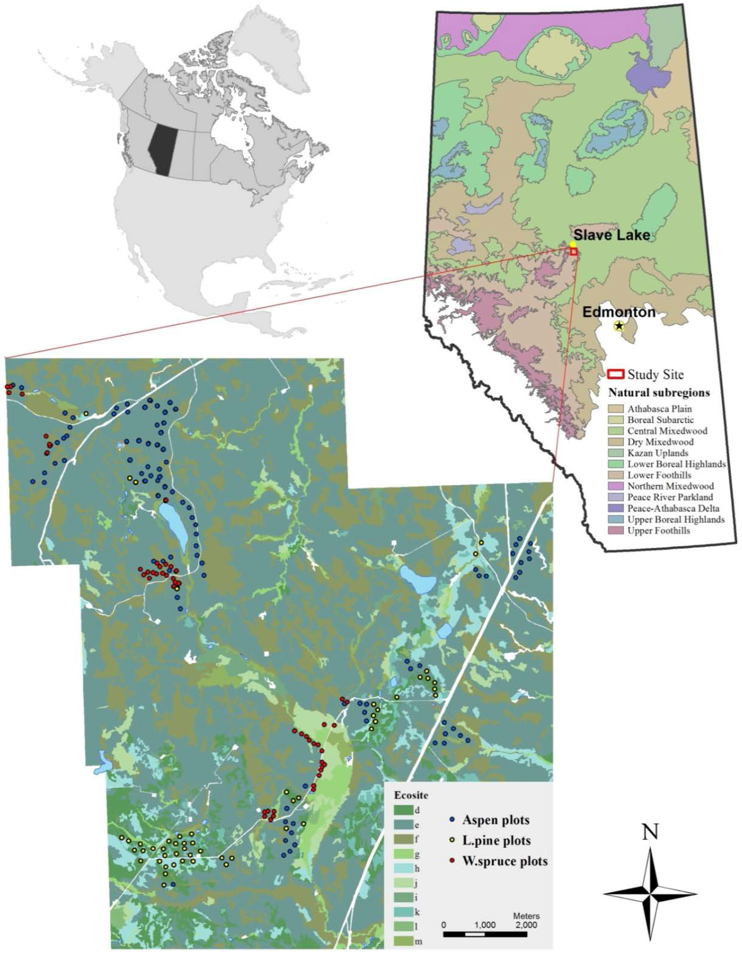
This study was conducted near Slave Lake in Central Alberta, Canada in the area of the 1968 Vega fire (Figure 1). This forested area is covered by mixed forests of trembling aspen, white spruce, and lodgepole pine, with an intermix of balsam poplar, white birch, black spruce, and tamarack. Topography is generally rolling, soils are predominantly Luvisols and Brunisols with gleyed variants and organic soils in poorly-drained conditions. The mean annual temperature is 2.4 °C, the mean temperature during the vegetation period (May–September) is 12.0 °C, there are 158 frost-free days, and the mean annual precipitation is 600 mm with 450 mm falling during the vegetation period (extracted from ClimateNA software for the period 1981–2010; [27]). The study area is relatively small in size (approx. 10 km in radius), and is located at the edge of the Lower Foothills Natural Subregion of Alberta [28]. This area has several advantages for a study designed to examine the relationships between ecological site factors and SI. Firstly, the area has a limited range of stand ages present, with most stands having originated after the 1968 fire, which places them close to the SI reference age (50 years). All stands have regenerated naturally with no evidence of management activities. The rolling topography provides a good range of site conditions and tree species. A case study in a geographically-restricted area like this, where climate is relatively constant across sites, provides some overall control of the macro-climate and allows us to focus on the effects of local topographic and soil factors. Finally, the ability to sample three major commercial tree species in the region—trembling aspen (Populus tremuloides Michx.), lodgepole pine (Pinus contorta Dougl. var. latifolia Engelm.), and white spruce (Picea glauca (Moench) Voss)—make this study of practical value.
Plot selection and tree selection criteria recommended in the SIBEC (Site Index Estimates by Biogeoclimatic Ecosystem Classification Site Series) Sampling and Data Standards [29] were followed. Based on these standards, areas selected for sampling were: even-aged stands; had moderate stand density; no management activities—natural stand conditions (e.g., no partial cuttings, fertilization, site preparation, pruning); not affected by major disturbances; appropriate ages (the closer to SI reference age of 50 years, the better); and contained suitable top height trees of target species. SIBEC selection criteria for top height trees were also used: the largest diameter dominant or co-dominant tree per 100 m2 was selected, provided it was vigorous, had a full crown, a straight, disease-free, undamaged stem (minor damage is allowed, but not which significantly affects tree growth), was free of suppression, and was not a wolf, open-grown, or veteran tree. In this region spruce regenerate and often grow in the understory; to verify that sampled spruce had not experienced suppression we checked the ring width close to the pith (early ages) and found no evidence of suppression and could, therefore, assume that these spruce trees satisfy the assumptions for SI estimation.
Aspen and lodgepole pine stands were selected for sampling based on: (1) dominant species; and (2) the range of DTW. Plot centres were then located randomly along predetermined transects within the selected areas to ensure sampling of the full range of DTW conditions available for each species. The center of measurement plots was adjusted from the point on the transect in order to ensure that site conditions were uniform within and around each plot, as required to meet plot and tree selection criteria. A buffer area of at least 50 m was left between sample plots and any disturbance or object (e.g., wellsite, road) to avoid edge effects. Neighbouring plots were located a minimum of 150–200 m apart and were situated in different site conditions (different slope, slope position, aspect, DTW, and/or SMR) in order to minimize correlations due to adjacency and ensure independence of plots. Due to restricted availability of white spruce stands we sampled all stands where we were able to select three unsuppressed top height trees while maintaining a minimum distance of 50 m from other sample plots and edges.
2.2. Data Collection and Variable Estimation
Data were collected within 300 m2 circular sample plots during 2014. Field sampling in each sample plot consisted of the determination of ecological data (topography parameters, soil properties, and stand density) and top height tree measurements to determine SI. A handheld Trimble GeoExplorer 6000 series GPS receiver (Trimble Inc., Sunnyvale, CA, USA) was used to ensure that ground plots accurately corresponded to remotely-sensed data sample plots. From the original dataset, aspen plots not affected (older than) by the recent fire, aspen in mixed stands, and spruce and pine plots with extreme DTW values (resulting in a large gap in the DTW range) were excluded from further analysis. This resulted in 97, 50, and 45 sample plots for trembling aspen, lodgepole pine, and white spruce, respectively. Table 1 shows the descriptive statistics for variables used in the analysis, while a summary of all stand and site attributes, including levels of categorical variables, are provided in Tables S1–S3 and Figures S1–S6.
2.2.1. Field Sampling Data
Top height tree measurements included diameter at breast height (DBH) and total height, while “bark-to-pith” increment cores were taken at breast height (1.3 m) for age determination. SI (height at a base age of 50 years total age for all species) was estimated for each selected top height tree using species-specific top height sub-models (height-age curves) of the GYPSY (Growth and Yield Projection System) forest growth and yield model [30], which is currently in use in Alberta. Given that GYPSY requires total age, the number of years for each tree to grow to breast height was first estimated using the same growth projections, and then added to ring counts from increment cores. SI at the plot level was calculated as the average of the values obtained from the top height trees in the plot, and used in subsequent analysis.
Determination of soil and topographic variables followed methods described in the Field Guide to Ecosites of West-central Alberta [28]. We transformed (“folded”) the aspect, so the coolest site has a value of zero and the warmest site has a value of 180. Following McCune and Keon [31] two methods were applied: (1) the folded aspect for incident radiation on the north–south line; and (2) the folded aspect for heat load using a northeast–southwest line. In each plot a soil pit was excavated at the plot centre to represent the average soil conditions in the plot, followed by field determination of major soil properties. Classification of soil characteristics consists of five levels for humus form, 14 levels for soil texture, four levels for effective soil texture, seven levels for drainage, nine levels for soil moisture regime, five levels for soil nutrient regime, and six levels for slope position.
2.2.2. Mapped Data
All digital environmental covariates were obtained from the high-resolution (1 m pixel size) bare-ground digital elevation model (DEM) and wet areas mapping (WAM). Both datasets were derived from airborne LiDAR point clouds obtained from flights during August–September 2008, with a mean return density of 1.7 points/m2 (ranging from 0.3 to 4.8 points/m2), acquired from the Alberta Ministry of Agriculture and Forestry. The depth-to-water (DTW) index and flow accumulation (FA) index provided by WAM were applied in the analysis. We used DTW rasters created from 0.5 ha, 1 ha, 2 ha, 4 ha, 6 ha, and 10 ha catchment areas (CA), which represents the size of the upslope contributing area required to initiate a stream flow. A DTW index integrates both slope and distance, which means landscape points further from open water bodies, both horizontally and vertically, have higher DTW values and drier soils [18], while FA is calculated as the upslope drainage area contributing to the point of interest and is expressed as the number contributing of cells (m2).
Built-in tools from the Spatial Analyst toolbox and Topography toolbox [32] in ArcGIS 10.1 were used to create corresponding surfaces. Two different indices were computed from the polar aspect, as explained above. The Topographic Wetness Index (TWI) is a widely-used topographically-based soil wetness model and represents the natural logarithm of the ratio of upslope flow accumulation area and slope [33]. The Discrete Slope Position Index (SPI) is classified based on the Topographic Position Index (TPI) and slope [34,35]. TPI compares the elevation of the standing (central) point and average elevation of the surrounding neighborhood, hence, it is scale-dependent. For this study we tested circular neighbourhood areas with seven different radiuses (from 5 to 100 m). The method classifies TPI into six slope position categories (crest, upper slope, middle slope, lower slope, flat, depression) based on standard deviation of the elevation and threshold (5°) of the slope to distinguish between midslope or flat areas. This approach to classifying slope position corresponds to the classification used in [28] for field surveys in Alberta, and allows a comparison between SPI maps derived from DEM data with field observations. Buffer areas of 15 and 20 m best corresponded to the field observations and, therefore, were selected as the most appropriate for the moderate (hilly) relief of the study area. Except for the Slope Position Index (SPI), which uses a buffer area in its calculation, all remotely-sensed variables were calculated at the plot level (averages at 300 m2 circular sample plot, but retaining original raster resolution), which corresponds to plot level values of the response, as suggested for the area-based approach to wall-to-wall prediction of forest inventory attributes [36]. Maps of the predicted SI were produced using the raster package [37] at 1 m resolution with plot level values assigned as grid cell values.
2.3. Statistical Analysis
We developed species-specific SI models (trembling aspen, lodgepole pine, and white spruce) from three different sets of explanatory variables: (1) all remotely-sensed variables; (2) only WAM variables; and (3) ground-based measured variables. Statistical analysis involved two major steps in terms of building SI prediction models: (1) correlation analysis was used in the selection of potential explanatory variables; and (2) variables most closely related to SI were used in modeling SI variation by applying four statistical approaches. Model optimization and comparison was based on absolute and relative measures of fit [38]: root mean squared error (RMSE), relative RMSE, coefficient of determination (R2), adjusted R2 (R2adj), Akaike information criteria (AIC), and Bayesian information criteria (BIC). The general rule for model selection (in the backward selection procedure) for all modeling methods was that a simpler model (with fewer parameters) was accepted if differences in R2adj were less than 2%. Regression diagnostic plots, such as residual plots and plots of measured versus predicted SI, were also examined. Due to this study having a spatially-clustered sampling design, model residuals were evaluated using a global Mantel test and correlogram [39] using the vegan package [40], which revealed no significant spatial autocorrelation issues (Figures S7–S9). Partial response curves were examined to evaluate the behaviour of each covariate included in the model in terms of ecological interpretability. All statistical analysis was completed using the R statistical software [41].
Correlation analysis was performed to explore the strength of the relationship between SI and environmental variables as the first step in variable selection for modeling. Variables that were significantly (p < 0.05) correlated with SI were selected for modeling. In addition, correlation analysis was used to select between collinear variables (τ > |0.7|). Kendall’s rank correlation coefficient (τ) was applied in correlation analysis for the majority of bivariate relationships, a quadratic relationship was also tested in cases where a non-monotonic relationship was observed among variables, while an optimal DTW index was selected based on Linear regression and generalized additive model fits.
A variety of different prediction techniques have been employed in the fine resolution extrapolation of point-based field observations of forest inventory attributes [42]. Methods used in modeling SI variation in response to environmental factors range from parametric to non-parametric [5,6,43,44,45,46]. We selected four statistical methods that have been successfully applied in SI-environment studies: (1) parametric—multiple linear regression; (2) semi-parametric—generalized additive models; (3) non-parametric (single regression tree-based method)—classification and regression trees; and (4) non-parametric (multiple regression tree-based method)—Random Forest.
Multiple linear regression (MLR) with backward selection was used to retain only variables with a significant slope parameter (p < 0.05). Best-subsets regression from the leaps package [47] was used in the backward selection procedure to screen the model and associated explanatory variables in order to determine the most important and optimal number of variables in the model. Selected environmental variables were linearized in cases when non-linear relationships with SI were evident. Interactions between the selected variables were also tested to evaluate their behaviour in the models. Multicollinearity and potential overfitting were assessed using variance inflation factors (VIF) assuming VIF < 5 overcomes the issues. Assumptions of normality and homogeneity of variance were tested on residuals, graphically, and using the Shapiro-Wilk test.
Generalized additive models (GAM) characterize the nature of the relationship between the response and predictors using multiple smoothing (non-linear) curve fits and, consequently, increases our understanding of ecological relationships [48]. However, the complexity of fitting the GAM model is in the selection of the optimal amount of smoothness. GAM modeling was done using the mgcv package [49]. We used generalized cross-validation techniques to optimize the smoothing level and the resulting smoothing (penalized) spline [50]. The following smoothness determination was applied: scatter plots with smoothing splines were examined for all variables to distinguish between linear and non-linear trends with SI; different smoothing functions and associated basis dimensions were then selected in order to achieve optimal fitting of the data; a penalized cubic regression spline function with shrinkage [50] was chosen with an upper limit of degrees of freedom was then applied to guard against over-smoothing, but still capture non-linear trends in the data; and, finally, smooth terms resulting in straight lines were switched to linear terms. Backward variable selection was used: poor predictors, and non-significant (p > 0.05) variables were dropped simultaneously; and then R2adj and BIC were used to select the optimal model.
Regression trees (RT) are descriptive and predictive models effective for discovering complex hierarchical interactions among predictors and non-linear relationships between predictor and response variables. With the predicted value as the mean of the observations in the terminal node [38], RT actually predicts classes because it is not fitted with a continuous smooth function. To grow regression trees we used the rpart package [51] with the splitting criteria and stopping criteria (minimum observations for each split attempt, minimum observations in any terminal node) and cross-validation set to default. Overall, splits were selected based on the predictor that resulted in maximizing between groups’ sum-of squares, accepted if overall R2 was improved by at least 1%, and the binary partitioning process was repeated for each new group (node) until the stopping criteria was reached. Pruning was applied to avoid overfitting based on a 10-fold cross-validation technique minimizing the cross-validation error [52].
Random Forest (RF) is a machine learning technique appropriate for multiple nonlinear regression analysis with accurate prediction power, the ability to detect variable interaction, the ability to measure variable importance, internal cross-validation, insensitivity to outliers, the ability to overcome collinearity, and a low tendency of overfitting as its advantages [53]. The randomForest package [54] was used, retaining defaults for random bootstrapping of the samples and variables. Hence, for each decision tree, about two-thirds of the samples were randomly selected as the training dataset, while the remaining samples were the ‘out-of-bag’ (OOB) samples used to calculate the mean squared prediction error (OOB error). After preliminary analysis the number of regression trees to grow was fixed to 3000 trees to ensure minimizing the OOB error. RMSE and the explained variance (pseudo R2) was computed based on averaged OOB error for all trees. We computed the variable importance measure of each predictor as given as the average percent change (before and after permutation) in the OOB error when the variable is permuted, while all others are retained unchanged. For model optimization, the backward variable selection approach [10] was applied minimizing the RMSE and maximizing the pseudo R2.
3. Results
3.1. Optimizing Size of Catchment Areas (CA) for Estimating SI
In order to determine optimal CA for use of the DTW index for modeling SI, six different CA (0.5, 1, 2, 4, 6, and 10 ha) were tested using two statistical methods, linear regression (LR) and generalized additive models (GAM), for the three investigated species. DTW for pine and spruce were log transformed prior to LR analysis, while GAM models were fitted with an upper limit of three degrees of freedom for aspen and spruce, and four for pine. Evaluation (using R2 for LR, and pseudo-R2 for GAM) of both modeling approaches (Figure 2) suggested that the resulting models showed very similar results and confirmed the strength and nature of the relationships between SI and DTW. Additionally, both methods provided similar inferences for each species in terms of the predictive capacity of DTW with different CA. Firstly, 0.5 ha had a smaller R2 than 1 ha CA for all species. Secondly, trends in R2 between 1 ha to 10 ha CA varied between species. For aspen, model performance peaked at 1 ha CA; for spruce, increasing the CA resulted in model improvement; while pine SI was insensitive to changes in the CA.
The non-linear trend for aspen (using the GAM model) peaks at around 1.95 m DTW_1 with SI of 22.2 m. Pine SI prediction models using DTW calculated at a 2 ha CA worked best for both GAM (R2 = 0.60) and LR (R2 = 0.63) models, with a sharp decrease at wet sites (DTW < 0.6 m) evident in the general logarithmic SI trend (Figure 3). Spruce SI was found to be best estimated using DTW at the largest tested catchment area of 10 ha, which accounted for 27% and 26% of the variation in SI based on a LR and GAM, respectively. Both fitted curves showed a positive relationship, but with different patterns, however, with the rise in SI being rapid from 0 to 2 m DTW_10 (Figure 3).
3.2. SI-Environment Relationship
Results from the correlation analysis (Tables S4–S7) were used to exclude variables having negligible effects on SI. TWI was dropped from further analysis due to its strong correlation with slope. Remotely-sensed topographic variables, except aspect, had moderate correlations with aspen SI with correlation coefficients ranging between 0.32 and 0.43. Declines in SI were associated with increases in DTW, altitude, slope, curvature, and slope position, and decreases in FA and TWI. Among the ground-based (field, GB) measured variables, only soil organic thickness was not significantly correlated with aspen SI. SMR and SNR were the most important soil variables (τ = 0.42 and 0.31, respectively), with SI being positively related to increases in SMR and SNR.
Pine SI was correlated with all remotely-sensed variables, but the strongest correlation was with DTW, warm aspects, steeper slope, convex surface, higher DTW, and topographic position, while lower altitude, FA, and TWI were associated with the most productive pine sites. Soil characteristics which significantly explained pine productivity were SNR and humus type. Pine growth was insensitive to soil texture, coarse fragment content, and soil organic layer thickness. The correlation between SI and SMR was not significant for pine due to the high variability of SI within well-drained mesic and submesic SMRs.
The strongest remotely-sensed variables correlated with spruce SI were DTW and altitude. While the positive trend in DTW might be plausible, increasing SI with altitude was unexpected. Weaker, but significant, nonlinear relationships were also detected for FA, aspect, slope, and slope position, with SI reaching a maximum at moderate conditions. Surface curvature indicators and TWI was not significantly related to spruce SI. Only four soil variables were significantly associated with spruce SI. Humus form appeared as the strongest (τ = −0.54), then DRN (τ = −0.24), while SMR, which peaked at mesic moisture conditions, was dropped due to its being strongly related to DRN. In addition, effective texture was a weak, but significant, explanatory variable, while SOT, CF, and SNR were uncorrelated with spruce SI.
Species-specific SI models were developed using four statistical methods. In addition, models were built using three sources of data: (1) remotely-sensed variables (RS), (2) only WAM variables, and (3) ground survey-based variables (GB). Selected models (Table 2) differ in explanatory variables, as well as in the number of variables for different species, data sources, and modeling methods. Aertsen et al. [6,44] also found differences in variables selected by five different modeling techniques applied to three species in two contrasting ecoregions, one where topographic factors control productivity, and one where soil properties control productivity. However, in our study DTW was the only variable selected by all statistical methods for each of the studied species (Table 2) and was also the most influential variable (Figure S10). In addition, the predominance of topographic parameters over field-determined soil variables is noticeable. Only the spruce GB SI model included, exclusively, soil variables (humus form and drainage), but topographic DTW and FA were also able to account for comparable amounts of the variation in spruce SI.
Biologically-plausible behaviour of each variable selected in the final models was evaluated based on relationships with SI and based on partial response curves (summarized in Table S8), confirming that the studied species respond differently to environmental factors. For instance, regression tree models (Figure S11), in addition to detecting complex interactions between environmental variables, revealed that the most productive sites for aspen (23.7 m SI) were found in sites with DTW below 10.9 m, convex surface curvature (<0.5), and lower altitude (<774 m). The most productive pine sites (SI = 16.8 m) had DTW above 0.8 m; and the most productive spruce stands (SI = 20.1 m) were at higher altitude (>830 m) with flat to midslope slope positions. Generally, for moisture-related variables (DTW, FA, slope, slope position, curvature, SMR, drainage), aspen SI increases with increasing moisture, but declines under conditions of excess water, pine SI declines with increasing moisture, while spruce SI reaches an optimum under moderate conditions (mesic SMR, midslope, etc.). These findings are also consistent with the close association between topographic features and soil moisture. Elevation was negatively related to aspen and pine SI, while it was positively related to spruce SI. Finally, higher nutrient availability (SNR and humus form) was associated with increases in productivity of all three species.
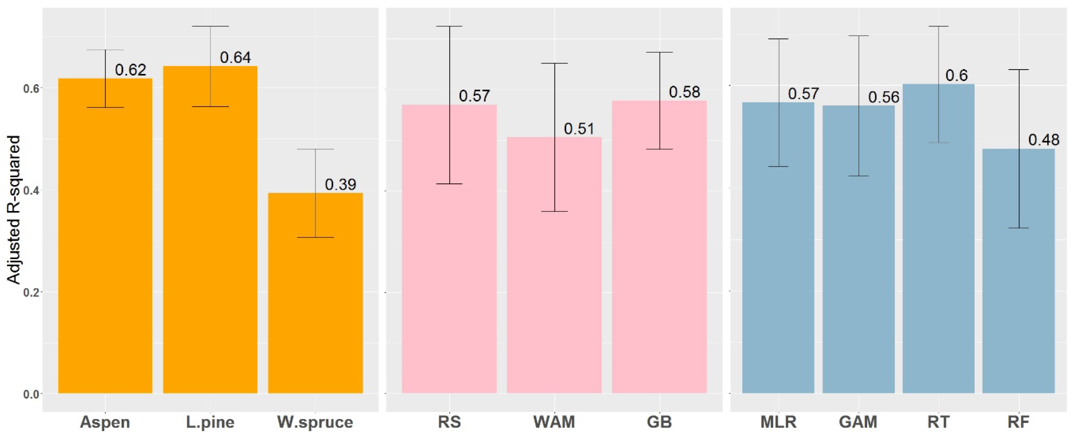
Differences in model prediction accuracy are evident between species, data sources, and statistical methods (Table 2). The best models accounted for between 63% and 70% of the variation in aspen SI (55–59% after bootstrapping for the Random Forest method), 66–73% of the variation in pine SI (63–64% for the RF method), and 34–50% of spruce SI variation (31–39% for the RF method). In terms of normalized RMSE, aspen models show higher predictive power than models for pine and spruce. No significant differences in variation explained were observed between models using remotely-sensed (average R2adj = 0.57) and ground-based variables (average R2adj = 0.58), while WAM data by itself (average R2adj = 0.51) explained most of the variation (Figure 4). Reported prediction accuracy for Random Forest was lower than that obtained using other methods, but this results from the use of fit statistics in RF that are calculated using cross-validation data.
4. Discussion
Divergence in the optimal CA for modeling different soil and vegetation characteristics using DTW is indicated by the range of values reported in the literature [19,20,21,24,55]. In this the foothills landscape is dominated by the fine textured glacial till parent material, and the strength of the relationship between SI and DTW differs with different CA for all three species (Figure 2). DTW based on smaller CA was better in estimating aspen SI, and the largest size (10 ha) of CA was the best for spruce, while the size of CA does not appear to have an influence for pine SI estimation. This is similar to findings of Oltean et al. [56] for aspen and spruce height in relation to DTW. Aspen SI appeared moisture-sensitive, with SMR (τ = 0.42) being the strongest ground-based SI predictor. Pine SI is not significantly correlated to SMR and DRN, but is strongly associated to SNR (τ = 0.51), which is, in turn, not related to DTW. Consequently, CA size was irrelevant for pine productivity estimation. For spruce SI, soil parameters, with HUM having the strongest correlation (τ = −0.54), were more important than topography. The results suggest that HUM is predicted better at larger CA, hence, 10 ha was the best CA for SI prediction. Generally, the results indicate that if the response is moisture-sensitive, then a lower CA is optimal, but when other factors drive the response, the optimal CA will vary. The optimal size of CA was also dependent on the response variable (application) [24]. Murphy et al. [19] found that the strongest relationship between soil properties and DTW was at the lowest tested CA. Different strengths of relationships between SI and the DTW index was found for different species (Figure 3). A weaker relationship for white spruce in our study is in line with the findings of Ung et al. [57]: SI models based on site factors were less accurate for shade-tolerant than for shade-intolerant species. However, different strengths of the relationship for aspen and pine likely result from limitations in field sampling, such as the captured ranges of the DTW index, the lack of full coverage of all ecosites, and the limited availability of areas to sample in extreme parts of the ranges of independent variables.
Aspen productivity depended strongly on environmental factors, as indicated by strong correlations between SI and almost all tested soil and topographic factors (Table S5). Other studies report similar relationships between aspen SI and soil moisture [56,57,58,59,60,61]. Excess water and conditions with poor soil aeration limit aspen growth [59,62,63], as also shown in our results. The maximum SI of aspen was found on sites with a subhygric soil moisture regime, flat to lower slope topographic position, and around 3 m DTW at 1 ha CA. Since it is a nutrient-demanding species, aspen growth was positively related to increasing SNR, as shown by other studies [58,59,61]. Higher aspen SI was found at lower altitudes and north aspects, which is also consistent with findings from other studies [58,59,60]. In our study, up to 70% of the variation in aspen SI was explained by environmental factors, similar to results from other studies in boreal forests. Chen et al. [58] reported strong relationships between SI and topographic indices (R2adj = 0.60), SMR, and SNR (R2adj = 0.63), and detailed soil physical and chemical properties (R2adj = 0.69) for northern British Columbia. Even stronger models were obtained for sites in the B.C. interior based on geographic position, elevation, SMR, and SNR (R2adj = 0.61), while the variance explained was 82% when biogeoclimatic zones were included in the model [59]. Stand characteristics and soil physical and chemical variables were found to improve parent material-specific aspen SI models with R2adj of 0.63 and 0.88 in Quebec [60] and R2adj from 0.45 to 0.54 in Saskatchewan [63].
Lodgepole pine SI was significantly correlated with several topographic variables and only with SNR and humus form among the soil variables. Although a dramatic decline in SI was noticed as the soil moisture increased from subhygric to subhydric, SMR and other soil physical properties were not significant in the models. This is likely due to pine being able to tolerate both very low and very high soil moisture levels, as well as a range of other site conditions, leading to substantial variability and a lack of a consistent general relationship between SI and SMR. A lack of samples at the extremes of SMR and a preponderance of plots in the submesic and mesic range may also be causing a weak relationship between SI and SMR. However, the significance of the slope position and DTW in the models using RS and WAM data may indicate issues relating to the subjective determination of SMR in the field. The results are consistent with findings by Wang et al. [8] that pine SI was negatively related to elevation, weakly associated with SNR, and not related to SMR. Additionally, Szwaluk et al. [4] reported that SNR and humus form were good SI predictors, and that soil physical variables were weaker in terms of explaining variance than soil chemical, understory plants, and humus form variables. In addition to climate factors, increasing fertility [64] and decreasing altitude [43] contributed significantly to explaining the variation in pine SI. Our results indicate that pine productivity was lowest at sites with poor nutrient regimes, higher altitude, lower topographic position (depression, level and lower slope), slight slope, low DTW, and high FA values. This is consistent with observations that good productivity of pine can be achieved on rocky soil, and steep slopes and ridges [62]. Up to 73% of the variation in pine SI was explained in this study. In a similar study in Southwestern Alberta, physical and chemical properties and understory vegetation explained up to 67% of the variation in SI [4]. Wang et al. [43] developed SI models for West-central Alberta, explaining up to 75% of the variation in SI using climate, topography, and soil sand content.
For white spruce, major factors influencing productivity were soil moisture (drainage and SMR), soil nutrient availability (humus form and SNR), DTW, and altitude. Slope position and FA were selected in final models, but they were weak predictors of SI. Humus form, in contrast to aspen and pine, was found to be the variable most closely related to SI. In terms of drainage and DTW_10 ha CA, decreases in moisture availability positively influenced spruce productivity. Interestingly, spruce grew best in sites with mesic SMR, and growth was lower in submesic and hygric sites, but inferences are limited because only two observations were sampled for submesic and hygric sites. SI was also highest on midslope sites and declined with increasing slope. Spruce SI also increased with increasing FA, but levelled off at high values. A non-monotonic relationship between SI and DTW calculated at lower CAs was also found. White spruce has a wide ecological amplitude, with limited growth in sites with stagnant water or under very dry conditions, and good productivity in sites with well-balanced water-aeration conditions [62]. While spruce is considered to be a nutrient-demanding species, SNR was not significant in our models due to the limited range of nutrient regimes sampled. Similar results were reported for sub-boreal white spruce where SMR was the strongest factor, with moderate moisture conditions having the highest SI, while SNR was less important [65]. Wang [66] found that soil physical properties were much better predictors of spruce SI than soil nutrient properties. Altitude was significant and was positively related to spruce SI. While other studies indicate that white spruce SI is insensitive to climate [65,67], interactions between elevation and the soil moisture regime may reflect the influence of climate on water availability and drought stress. Stand attributes, including composition and age effects, have been found to be important in SI predictions for shade-tolerant species [57], such as white spruce, leading to increases in variability in SI under different environmental conditions. An age trend for spruce SI indicates a possible violation of assumptions for SI determination. This could be due to competition effects in young stands which are common for shade-tolerant white spruce, or to a poor fit of the height age curves used for these particular stands. This has been noted as a potential issue in several other similar studies [61,68,69,70] with changes in climate and fertility over time often being given as an explanation for this violation of the assumption of time independence for SI estimates.
Models developed in this study accounted for up to 73%, 70%, and 50% of the variation in SI for pine, aspen, and spruce, respectively. Generally, SI prediction models explain between 50% and 80% of the SI variation in models built from local site factors [12]. The results from our study fall within this range, but with pine and aspen reaching the upper limit, and spruce approaching the lower end of this range (Figure 4, left plot). Site factors important for spruce growth not included in the study, or issues relating to stand ages and sampling design, might cause poorer results for spruce than for aspen and pine. Comparing results from different modeling approaches across all species, average R2adj values were very similar between RS and GB variables (Figure 4, middle plot). In addition, although it provided lower R2adj, WAM data by itself was able to explain most of the variation in SI. In terms of best predictors, among RS variables DTW was selected by each statistical method for each species and, in most cases, it is the strongest predictor in the model, while, for GB data, different variables appeared as the most important for each species according to species silvics. For DTW, GAM provided a more plausible fit for aspen and MLR was able to better detect logarithmic trends for pine.
Several different methods for developing SI prediction models have been suggested in the literature. Although RT models tended to overfit when only two WAM variables were used, little difference is apparent between MLR, GAM, and RT methods in terms of the explained variance (Figure 4, right plot). RF gave poorer results due to different statistics being used for comparison, but the results are still comparable. Non-parametric models show some bias in terms of predicting higher values for less productive sites and lower values in more productive sites (Figures S12–S14). A slightly different fit was found as a result of differences in the representation of nonlinearity between MLR and GAM models, however, similarity in covariate behaviour in the models from different methods was confirmed by the form of relationships for each of the three species. Our findings are consistent with recommendations that the preference for SI prediction be given to GAM in terms of predictive performance [43], as well as to GAM and non-parametric Boosted Regression Trees in terms of fit statistics and ecological interpretability [6,44]. When spatial autocorrelation issues arise, a sequential autoregressive spatial regression modeling approach may be superior to other methods [71,72].
Maps of SI for each species are shown in Figure 5, Figure 6 and Figure 7. Despite some differences in predictions due to model specifics, relationships between terrain attributes and patterns of low and high predicted productivity are generally apparent. However, some issues related to spatial predictions exist. Firstly, extrapolating outside the range of training data, as well as outside of the study area, is risky and can result in unreliable estimates [73]. Nonparametric regression tree-based methods used in our study are data-driven and provide categorical outcomes, so when applied outside of the range of training data they predict the same classes as found in the training dataset [73]. Another difference between MLR and GAM models for the aspen SI maps is evident for predictions along streams (out of range for low DTW and high FA) where MLR tends to overpredict SI due to a negative linear fit for DTW and a positive logarithmic fit for FA, while the GAM model exhibits a more plausible decrease in SI at low DTW and high FA values. A similar pattern in spruce SI prediction is evident at higher elevations (and higher DTW) with the GAM method producing much larger values and larger areas of high SI (>20 m) due to the positive relationship between SI and DTW. In order to develop biologically-sound SI models predicted from contemporary and future climate projections Antón-Fernández et al. [9] applied a modeling technique based on the potential modifier functional form which bounds the response within a specified observed range. Further, spatial SI predictions illustrate fine differences when using different types (discrete/categorical vs. continuous) and the numbers of explanatory variables. MLR and GAM provide a continuous fit throughout the range of response and ecologically-plausible mapping. For RT, a drawback is that the estimates represent classes which result in spatial prediction being fragmented [43]. Where there are a small number of classes with unequal differences between classes, resulting predictions may not be realistic, as observed for the aspen RT model where the application of a DTW threshold of 10.9 m assigns SI values of 18 m and 22 m to neighbouring cells. However, RT might be appropriate for SI predictions at large scales with large datasets [73].
Forest productivity is affected by complex interactions between site factors, species autecology, genetic variability, and management practices and, as a result, it is often difficult to assess [74]. Biophysical SI models usually have moderate accuracy and rarely explain more than 80% of the variance. However, computation of SI is subject to errors in height and age determination. In addition, applying provincial or regional SI curves might not account for regional differences in growth. Growth factors not accounted for in the models include detailed soil attributes and extreme abiotic or biotic factors, including diseases, insects, and genetics [75]. Adding explanatory variables obtained from more detailed ecological surveys and laboratory analysis of soil and foliage might improve productivity predictions, but would involve increases in sampling costs and decreases in model effectiveness.
5. Conclusions
We demonstrate the usefulness of WAM variables for accurate and high-resolution estimation of SI, revealing that the DTW index is the strongest DEM-derived SI predictor and that the FA index can explain the influence of other important soil properties in our study area. Models developed in this study accounted for up to 73%, 70%, and 50% of variation in SI for pine, aspen, and spruce, respectively. Poorer results for spruce result from the wide range in ages of sampled spruce stands, the lack of spruce stands across a full range of sites, and the small number of spruce stands where top height trees free of suppression could be sampled. No differences in the explained variation were observed between models based on data from remote sensing or field assessment, while WAM data by itself explained most of the variation in SI. High-resolution SI maps for all species were produced and, despite some general issues, show plausible relationships between terrain attributes and productivity and, hence, are potentially applicable for operational-scale forest growth and yield modeling. However, further refinements in SI prediction models might be possible by utilizing first-return LiDAR metrics [45] and optical imagery.
Supplementary Materials
The following are available online at https://www.mdpi.com/1999-4907/9/3/113/s1; Table S1: Summary of stand attributes for the three studied tree species; Table S2: Summary of remotely-sensed variables considered in modeling SI by the studied tree species; Table S3: Summary of the ground-measured variables considered in modeling SI by the studied tree species; Table S4: Kendall’s rank correlation coefficient (τ) matrix between remotely-sensed environmental and soil attributes (N = 201). Bolded numbers indicate the significance of relationship at p < 0.05; Table S5: Kendall’s rank correlation coefficient (τ) matrix between aspen SI and environmental variables (N = 97). Bolded numbers indicate the significance of the relationship at p < 0.05. Italicized numbers indicate the coefficient of determination from quadratic regression; Table S6: Kendall’s rank correlation coefficient (τ) matrix between lodgepole pine SI and environmental variables (N = 50). Bolded numbers indicate the significance of the relationship at p < 0.05 (* p = 0.06). Italicized numbers indicate the coefficient of determination from quadratic regression; Table S7: Kendall’s rank correlation coefficient (τ) matrix between white spruce SI and environmental variables (N = 45). Bolded numbers indicate the significance of the relationship at p < 0.05. Italicized numbers indicate the coefficient of determination from quadratic regression (* exponential transformation); Table S8: Summary by species of responses in SI on site factors included in the final models; ⬆—positive, ⬇—negative, ➡—no response, ( )—trend detected only by some statistical methods, * no significant relationship between SI and single particular predictor; Figure S1: Box plots with jitter plots of SI and environmental (remotely-sensed and ground-based measured) variables for aspen. Black dots represent the mean; Figure S2: Box plots with jitter plots of SI and environmental (remotely-sensed and ground-based measured) variables for lodgepole pine. The black dot represents the mean; Figure S3: Box plots with jitter plots of SI and environmental (remotely-sensed and ground-based measured) variables for white spruce. Black dots represent the mean; Figure S4: Scatter plots with penalized regression spline (three degrees of freedom) between environmental (remotely-sensed and ground-based measured) variables and SI for aspen; Figure S5: Scatter plots with penalized regression spline (three degrees of freedom) between environmental (remotely-sensed and ground-based measured) variables and SI for lodgepole pine; Figure S6: Scatter plots with penalized regression spline (three degrees of freedom) between environmental (remotely-sensed and ground-based measured) variables and SI for white spruce; Figure S7; Spatial correlation structure for aspen presented using Mantel correlograms on model residuals based on the Euclidian distance method. Black squares indicate significant (p < 0.05) spatial correlation at corresponding distance classes; Figure S8: Spatial correlation structure for lodgepole pine presented using Mantel correlograms on model residuals based on the Euclidian distance method. Black squares indicate significant (p < 0.05) spatial correlation at corresponding distance classes; Figure S9: Spatial correlation structure for white spruce presented using Mantel correlograms on model residuals based on the Euclidian distance method. Black squares indicate significant (p < 0.05) spatial correlation at corresponding distance classes; Figure S10: Variable importance plots for aspen (A,B), pine (C,D), and spruce (E,F) SI Random Forest models built with all potential remotely-sensed (A,C,E) and ground-based measured (B,D,F) variables. %IncMSE—variable importance measure indicating the average percent change in the mean square error when the particular variable is removed while all others are retained unchanged. Important variables should cause relatively large %IncMSE; Figure S11: Regression Tree SI models based on remotely-sensed data; (A) aspen, (B) lodgepole pine, and (C) white spruce; Figure S12: Residual and measured vs. predicted plots for aspen by data sources and modeling techniques. The 1:1 line is shown in red; Figure S13: Residual and measured vs. predicted plots for pine by data sources and modeling techniques. The 1:1 line is shown in red; Figure S14: Residual and measured vs. predicted plots for spruce by data sources and modeling techniques. The 1:1 line is shown in red.
Acknowledgments
We gratefully acknowledge the financial contributions from Alberta Agriculture and Forestry that made this study possible. We would also like to acknowledge valuable contributions by the Forest Watershed Research Centre located at the University of New Brunswick, and particularly by Jae Ogilvie, who kindly provided the wet areas mapping products used in this study. We are grateful to Alberta Plywood Ltd. and Greenlink Forestry Inc. for providing access to vegetation inventory data of the research area, and to Craig Cruikshank who assisted with the fieldwork.
Author Contributions
P.G.C. and B.W. conceived and designed the study; I.B. performed field sampling and analyzed the data with contributions from P.G.C.; and I.B. wrote the paper with contributions from P.G.C. and B.W.
Conflicts of Interest
The authors declare no conflict of interest.
References
- Skovsgaard, J.P.; Vanclay, J.K. Forest site productivity: A review of the evolution of dendrometric concepts for even-aged stands. Forestry 2008, 81, 13–31. [Google Scholar] [CrossRef]
- Farrelly, N.; Dhubhain, A.N.; Nieuwenhuis, M. Sitka spruce site index in response to varying soil moisture and nutrients in three different climate regions in Ireland. For. Ecol. Manag. 2011, 262, 2199–2206. [Google Scholar] [CrossRef]
- Aertsen, W.; Kint, V.; de Vos, B.; Deckers, J.; van Orshoven, J.; Muys, B. Predicting forest site productivity in temperate lowland from forest floor, soil and litterfall characteristics using boosted regression trees. Plant Soil 2012, 354, 157–172. [Google Scholar] [CrossRef]
- Szwaluk, K.S.; Strong, W.L. Near-surface soil characteristics and understory plants as predictors of Pinus contorta site index in southwestern Alberta, Canada. For. Ecol. Manag. 2003, 176, 13–24. [Google Scholar] [CrossRef]
- Subedi, S.; Fox, T.R. Predicting Loblolly Pine Site Index from Soil Properties Using Partial Least-Squares Regression. For. Sci. 2016, 62, 449–456. [Google Scholar] [CrossRef]
- Aertsen, W.; Kint, V.; van Orshoven, J.; Özkan, K.; Muys, B. Comparison and ranking of different modelling techniques for prediction of site index in Mediterranean mountain forests. Ecol. Model. 2010, 221, 1119–1130. [Google Scholar] [CrossRef]
- Socha, J. Effect of topography and geology on the site index of Picea abies in the West Carpathian, Poland. Scand. J. For. Res. 2008, 23, 203–213. [Google Scholar] [CrossRef]
- Wang, G.G.; Huang, S.; Monserud, R.A.; Klos, R.J. Lodgepole pine site index in relation to synoptic measures of climate, soil moisture and soil nutrients. For. Chron. 2004, 80, 678–686. [Google Scholar] [CrossRef]
- Antón-Fernández, C.; Mola-Yudego, B.; Dalsgaard, L. Climate sensitive site index models for Norway. Can. J. For. Res. 2016, 46, 794–803. [Google Scholar] [CrossRef]
- Weiskittel, A.; Crookston, N.; Radtke, P. Linking climate, gross primary productivity, and site index across forests of the western United States. Can. J. For. Res. 2011, 41, 1710–1721. [Google Scholar] [CrossRef]
- Monserud, R.A.; Huang, S.; Yang, Y. Predicting lodgepole pine site index from climatic parameters in Alberta. For. Chron. 2006, 82, 562–571. [Google Scholar] [CrossRef]
- Bontemps, J.-D.; Bouriaud, O. Predictive approaches to forest site productivity: Recent trends, challenges and future perspectives. Forestry 2014, 87, 109–128. [Google Scholar] [CrossRef]
- Iverson, L.R.; Dale, M.E.; Scott, C.T.; Prasad, A. A GIS-derived integrated moisture index to predict forest composition and productivity of Ohio forests (U.S.A.). Landsc. Ecol. 1997, 12, 331–348. [Google Scholar] [CrossRef]
- Berrill, J.P.; O’Hara, K.L. How do biophysical factors contribute to height and basal area development in a mixed multiaged coast redwood stand? Forestry 2016, 89, 170–181. [Google Scholar] [CrossRef]
- Mitsuda, Y.; Ito, S.; Sakamoto, S. Predicting the site index of sugi plantations from GIS-derived environmental factors in Miyazaki Prefecture. J. For. Res. 2007, 12, 177–186. [Google Scholar] [CrossRef]
- Laamrani, A.; Valeria, O.; Bergeron, Y.; Fenton, N.; Cheng, L.Z.; Anyomi, K. Effects of topography and thickness of organic layer on productivity of black spruce boreal forests of the canadian clay belt region. For. Ecol. Manag. 2014, 330, 144–157. [Google Scholar] [CrossRef]
- White, B.; Ogilvie, J.; Campbell, D.M.H.; Hiltz, D.; Gauthier, B.; Chisholm, H.K.; Wen, H.K.; Murphy, P.N.C.; Arp, P.A. Using the Cartographic Depth-to-Water Index to Locate Small Streams and Associated Wet Areas across Landscapes. Can. Water Resour. J. 2012, 37, 333–347. [Google Scholar] [CrossRef]
- Murphy, P.N.C.; Ogilvie, J.; Arp, P. Topographic modelling of soil moisture conditions: A comparison and verification of two models. Eur. J. Soil Sci. 2009, 60, 94–109. [Google Scholar] [CrossRef]
- Murphy, P.N.C.; Ogilvie, J.; Meng, F.R.; White, B.; Bhatti, J.S.; Arp, P.A. Modelling and mapping topographic variations in forest soils at high resolution: A case study. Ecol. Model. 2011, 222, 2314–2332. [Google Scholar] [CrossRef]
- Ågren, A.M.; Lidberg, W.; Strömgren, M.; Ogilvie, J.; Arp, P.A. Evaluating digital terrain indices for soil wetness mapping—A Swedish case study. Hydrol. Earth Syst. Sci. Discuss. 2014, 11, 4103–4129. [Google Scholar] [CrossRef]
- Oltean, G.S.; Comeau, P.G.; White, B. Linking the Depth-to-Water Topographic Index to Soil Moisture on Boreal Forest Sites in Alberta. For. Sci. 2016, 62, 154–165. [Google Scholar] [CrossRef]
- Hiltz, D.; Gould, J.; White, B.; Ogilvie, J.; Arp, P. Modeling and mapping vegetation type by soil moisture regime across boreal landscapes. In Restoration and Reclamation of Boreal Ecosystems: Attaining Sustainable Development; Cambridge University Press: New York, NY, USA, 2012; pp. 56–75. [Google Scholar]
- Nijland, W.; Nielsen, S.E.; Coops, N.C.; Wulder, M.A.; Stenhouse, G.B. Fine-spatial scale predictions of understory species using climate- and LiDAR-derived terrain and canopy metrics. J. Appl. Remote Sens. 2014, 8, 083572. [Google Scholar] [CrossRef]
- Nijland, W.; Coops, N.C.; Macdonald, S.E.; Nielsen, S.E.; Bater, C.W.; White, B.; Ogilvie, J.; Stadt, J. Remote sensing proxies of productivity and moisture predict forest stand type and recovery rate following experimental harvest. For. Ecol. Manag. 2015, 357, 239–247. [Google Scholar] [CrossRef]
- Hennigar, C.; Weiskittel, A.; Allen, H.L.; MacLean, D.A. Development and evaluation of a biomass increment-based index for site productivity. Can. J. For. Res. 2017, 47, 400–410. [Google Scholar] [CrossRef]
- Parresol, B.R.; Scott, D.A.; Zarnoch, S.J.; Edwards, L.A.; Blake, J.I. Modeling forest site productivity using mapped geospatial attributes within a South Carolina Landscape, USA. For. Ecol. Manag. 2017, 406, 196–207. [Google Scholar] [CrossRef]
- Wang, T.; Hamann, A.; Spittlehouse, D.L.; Murdock, T.Q. ClimateWNA-high-resolution spatial climate data for western North America. J. Appl. Meteorol. Climatol. 2012, 51, 16–29. [Google Scholar] [CrossRef]
- Beckingham, J.D.; Corns, I.G.W.; Archibald, J.H. Field Guide to Ecosites of West-Central Alberta; Natural Resources Canada, Canadian Forest Service, Northern Forestry Centre: Edmonton, AB, Canada, 1996. [Google Scholar]
- SIBEC Sampling and Data Standards. Available online: https://www2.gov.bc.ca/assets/gov/environment/plants-animals-and-ecosystems/ecosystems/sibec-documents/standards.pdf (accessed on 1 March 2018).
- Huang, S.; Meng, S.X.; Yang, Y. A Growth and Yield Projection System (GYPSY) for Natural and Post-harvest Stands in Alberta. Alta. Sustain. Resour. Dev. Tech. Rep. 2009, T/216, 1–22. [Google Scholar]
- McCune, B.; Keon, D. Equations for potential annual direct incident radiation and heat load. J. Veg. Sci. 2002, 13, 603–606. [Google Scholar] [CrossRef]
- Dilts, T.E. Topography Tools for ArcGIS 10.1. Available online: http://www.arcgis.com/home/item.html?id=b13b3b40fa3c43d4a23a1a09c5fe96b9 (accessed on 1 March 2018).
- Beven, K.J.; Kirkby, M.J. A physically based, variable contributing area model of basin hydrology. Hydrol. Sci. Bull. 1979, 24, 43–69. [Google Scholar] [CrossRef]
- Weiss, A. Topographic position and landforms analysis. Poster Present. ESRI User Conf. San Diego CA 2001, 64, 227–245. [Google Scholar]
- Jenness, J. Some Thoughts on Analyzing Topographic Habitat Characteristics. Available online: http://www.jennessent.com/downloads/topographic_analysis_online.pdf (accessed on 1 March 2018).
- White, J.C.; Wulder, M.A.; Varhola, A.; Vastaranta, M.; Coops, N.C.; Cook, B.D.; Pitt, D.; Woods, M. A best practices guide for generating forest inventory attributes from airborne laser scanning data using an area-based approach. For. Chron. 2013, 89, 722–723. [Google Scholar] [CrossRef]
- Hijmans, R.; van Etten, J.; Cheng, J.; Mattiuzzi, M.; Sumner, M.; Greenberg, J.A.; Lamigueiro, O.; Bevan, A.; Racine, E.; Shortridge, A.; et al. Raster: Geographic Data Analysis and Modeling. Available online: http://cran.r-project.org/package=raster (accessed on 1 March 2018).
- Quinn, G.P.; Keough, M.J. Experimental Design and Data Analysis for Biologists; Cambridge University Press: New York, NY, USA, 2002; p. 537. [Google Scholar]
- Borcard, D.; Gillet, F.; Legendre, P. Numerical Ecology with R; Springer: New York, NY, USA, 2011; ISBN 9780387938363. [Google Scholar]
- Oksanen, J.; Blanchet, F.G.; Friendly, M.; Kindt, R.; Legendre, P.; Mcglinn, D.; Minchin, P.R.; O’hara, R.B.; Simpson, G.L.; Solymos, P.; et al. Vegan: Community Ecology Package. Available online: https://CRAN.R-project.org/package=vegan (accessed on 1 March 2018).
- The R Project for Statistical Computing. Available online: http://www.R-project.org/ (accessed on 1 March 2018).
- Brosofske, K.D.; Froese, R.E.; Falkowski, M.J.; Banskota, A. A review of methods for mapping and prediction of inventory attributes for operational forest management. For. Sci. 2014, 60, 733–756. [Google Scholar] [CrossRef]
- Wang, Y.; Raulier, F.; Ung, C.H. Evaluation of spatial predictions of site index obtained by parametric and nonparametric methods—A case study of lodgepole pine productivity. For. Ecol. Manag. 2005, 214, 201–211. [Google Scholar] [CrossRef]
- Aertsen, W.; Kint, V.; Van Orshoven, J.; Muys, B. Evaluation of modelling techniques for forest site productivity prediction in contrasting ecoregions using stochastic multicriteria acceptability analysis (SMAA). Environ. Model. Softw. 2011, 26, 929–937. [Google Scholar] [CrossRef] [Green Version]
- Watt, M.S.; Dash, J.P.; Bhandari, S.; Watt, P. Comparing parametric and non-parametric methods of predicting Site Index for radiata pine using combinations of data derived from environmental surfaces, satellite imagery and airborne laser scanning. For. Ecol. Manag. 2015, 357, 1–9. [Google Scholar] [CrossRef]
- Sabatia, C.O.; Burkhart, H.E. Predicting site index of plantation loblolly pine from biophysical variables. For. Ecol. Manag. 2014, 326, 142–156. [Google Scholar] [CrossRef]
- Lumley, T. Leaps: Regression Subset Selection. Available online: https://CRAN.R-project.org/package=leaps (accessed on 1 March 2018).
- Guisan, A.; Edwards, T.C.; Hastie, T. Generalized linear and generalized additive models in studies of species distributions: Setting the scene. Ecol. Model. 2002, 157, 89–100. [Google Scholar] [CrossRef]
- Wood, A.S.; Wood, M.S. Mgcv: Mixed GAM Computation Vehicle with Automatic Smoothness Estimation. Available online: https://cran.r-project.org/web/packages/mgcv/index.html (accessed on 1 March 2018).
- Zuur, A.F.; Ieno, E.N.; Walker, N.J.; Saveliev, A.A.; Smith, G.M. Mixed Effects Models and Extensions in Ecology with R; Statistics Biology Health Springer: New York, NY, USA, 2009; 579p. [Google Scholar]
- Therneau, T.; Atkinson, B.; Ripley, B.; Ripley, M.B. Rpart: Recursive Partitioning and Regression Trees. Available online: https://cran.r-project.org/web/packages/rpart/index.html (accessed on 1 March 2018).
- Maindonald, J.; Braun, W.J. Data Analysis and Graphics Using R—An Example-Based Approach, 3rd ed.; Cambridge University Press: New York, NY, USA, 2003; p. 565. [Google Scholar]
- Breiman, L. Random forests. Mach. Learn. 2001, 5–32. [Google Scholar] [CrossRef]
- Liaw, A.; Wiener, M.; Andy Liaw, M. randomForest: Breiman and Cutler’s Random Forests for Classification and Regression. Available online: http://cran.r-project.org/package=randomForest (accessed on 1 March 2018).
- Campbell, D.M.H.; White, B.; Arp, P.A. Modeling and mapping soil resistance to penetration and rutting using LiDAR-derived digital elevation data. J. Soil Water Conserv. 2013, 68, 460–473. [Google Scholar] [CrossRef]
- Oltean, G.S.; Comeau, P.G.; White, B. Carbon isotope discrimination by Picea glauca and Populus tremuloides is related to the topographic depth to water index and rainfall. Can. J. Res. 2016, 46, 1225–1233. [Google Scholar] [CrossRef]
- Ung, C.H.; Bernier, P.Y.; Raulier, F.; Fournier, R.A.; Lambert, M.C.; Régnière, J. Biophysical site indices for shade tolerant and intolerant boreal species. For. Sci. 2001, 47, 83–95. [Google Scholar]
- Chen, H.Y.; Klinka, K.; Kabzems, R.D. Site index, site quality, and foliar nutrients of trembling aspen: Relationships and predictions. Can. J. For. Res. 1998, 28, 1743–1755. [Google Scholar] [CrossRef]
- Chen, H.Y.; Krestov, P.V.; Klinka, K. Trembling aspen site index in relation to environmental measures of site quality at two spatial scales. Can. J. For. Res. 2002, 32, 112–119. [Google Scholar] [CrossRef]
- Pinno, B.D.; Paré, D.; Guindon, L.; Bélanger, N. Predicting productivity of trembling aspen in the Boreal Shield ecozone of Quebec using different sources of soil and site information. For. Ecol. Manag. 2009, 257, 782–789. [Google Scholar] [CrossRef]
- Anyomi, K.A.; Lorenzetti, F.; Bergeron, Y.; Leduc, A. Stand Dynamics, Humus Type and Water Balance Explain Aspen Long Term Productivity across Canada. Forests 2015, 6, 416–432. [Google Scholar] [CrossRef]
- Burns, R.M.; Honkala, B.H. Silvics of North America: 1. Conifers; 2. Hardwoods; United States Department of Agriculture: Washington, DC, USA, 1990; Volume 2, p. 877.
- Pinno, B.D.; Bélanger, N. Estimating trembling aspen productivity in the boreal transition ecoregion of saskatchewan using site and soil variables. Can. J. Soil Sci. 2011, 91, 661–669. [Google Scholar] [CrossRef] [Green Version]
- Fries, A.; Lindgren, D.; Ying, C.C.; Ruotsalainen, S.; Lindgren, K.; Elfving, B.; Karlmats, U. The effect of temperature on site index in western Canada and Scandinavia estimated from IUFRO Pinus contorta provenance experiments. Can. J. For. Res. 2000, 30, 921–929. [Google Scholar] [CrossRef]
- Wang, G.G.; Klinka, K. Use of synoptic variables in predicting white spruce site index. For. Ecol. Manag. 1996, 80, 95–105. [Google Scholar] [CrossRef]
- Wang, G.G. White spruce site index in relation to soil, understory vegetation, and foliar nutrients. Can. J. For. Res. 1995, 25, 29–38. [Google Scholar] [CrossRef]
- Nigh, G.D.; Ying, C.C.; Qian, H. Climate and Productivity of Major Conifer Species in the Interior of British Columbia, Canada. For. Sci. 2004, 50, 659–671. [Google Scholar]
- Albert, M.; Schmidt, M. Climate-sensitive modelling of site-productivity relationships for Norway spruce (Picea abies (L.) Karst.) and common beech (Fagus sylvatica L.). For. Ecol. Manag. 2010, 259, 739–749. [Google Scholar] [CrossRef]
- Anyomi, K.A.; Raulier, F.; Bergeron, Y.; Mailly, D. The predominance of stand composition and structure over direct climatic and site effects in explaining aspen (Populus tremuloides Michaux) site index within boreal and temperate forests of western Quebec, Canada. For. Ecol. Manag. 2013, 302, 390–403. [Google Scholar] [CrossRef]
- Aertsen, W.; Kint, V.; Muys, B.; Van Orshoven, J. Effects of scale and scaling in predictive modelling of forest site productivity. Environ. Model. Softw. 2012, 31, 19–27. [Google Scholar] [CrossRef]
- Latta, G.; Temesgen, H.; Barrett, T.M. Mapping and imputing potential productivity of Pacific Northwest forests using climate variables. Can. J. For. Res. 2009, 39, 1197–1207. [Google Scholar] [CrossRef]
- Zald, H.S.J.; Spies, T.A.; Seidl, R.; Pabst, R.J.; Olsen, K.A.; Steel, E.A. Complex mountain terrain and disturbance history drive variation in forest aboveground live carbon density in the western Oregon Cascades, USA. For. Ecol. Manag. 2016, 366, 193–207. [Google Scholar] [CrossRef] [PubMed]
- McKenney, D.W.; Pedlar, J.H. Spatial models of site index based on climate and soil properties for two boreal tree species in Ontario, Canada. For. Ecol. Manag. 2003, 175, 497–507. [Google Scholar] [CrossRef]
- Weiskittel, A.R.; Hann, D.W.; Kershaw, J.; Vanclay, J.K. Forest Growth and Yield Modeling; John Wiley & Sons: Hoboken, NJ, USA, 2011. [Google Scholar]
- Latutrie, M.; Mérian, P.; Picq, S.; Bergeron, Y.; Tremblay, F. The effects of genetic diversity, climate and defoliation events on trembling aspen growth performance across Canada. Tree Genet. Genomes 2015, 11, 96. [Google Scholar] [CrossRef]
Figure 1.
Study site location and Natural subregions (forested) of Alberta (upper right map). Sample plot locations and ecosite map of the study site (lower map). Final sample size of 97, 50, and 45 plots were for trembling aspen, lodgepole pine, and white spruce, respectively. Ecosite (Lower Foothlls Natural Subregion [28]) abbreviations: d—Labrador tea-mesic; e—low-bush cranberry; f—bracted honeysuckle; g—meadow; h—Labrador tea-subhygric; i—horsetail; j—Labrador tea/horsetail; k—bog; l—poor fen; and m—rich fen.

Figure 2.
SI variation explained (R2) by DTW calculated at six different WAM catchment areas (CA) by species and statistical approaches. SI: site index; DTW: depth-to-water; WAM: wet areas mapping; LR: linear regression; GAM: generalized additive models.
Figure 2.
SI variation explained (R2) by DTW calculated at six different WAM catchment areas (CA) by species and statistical approaches. SI: site index; DTW: depth-to-water; WAM: wet areas mapping; LR: linear regression; GAM: generalized additive models.
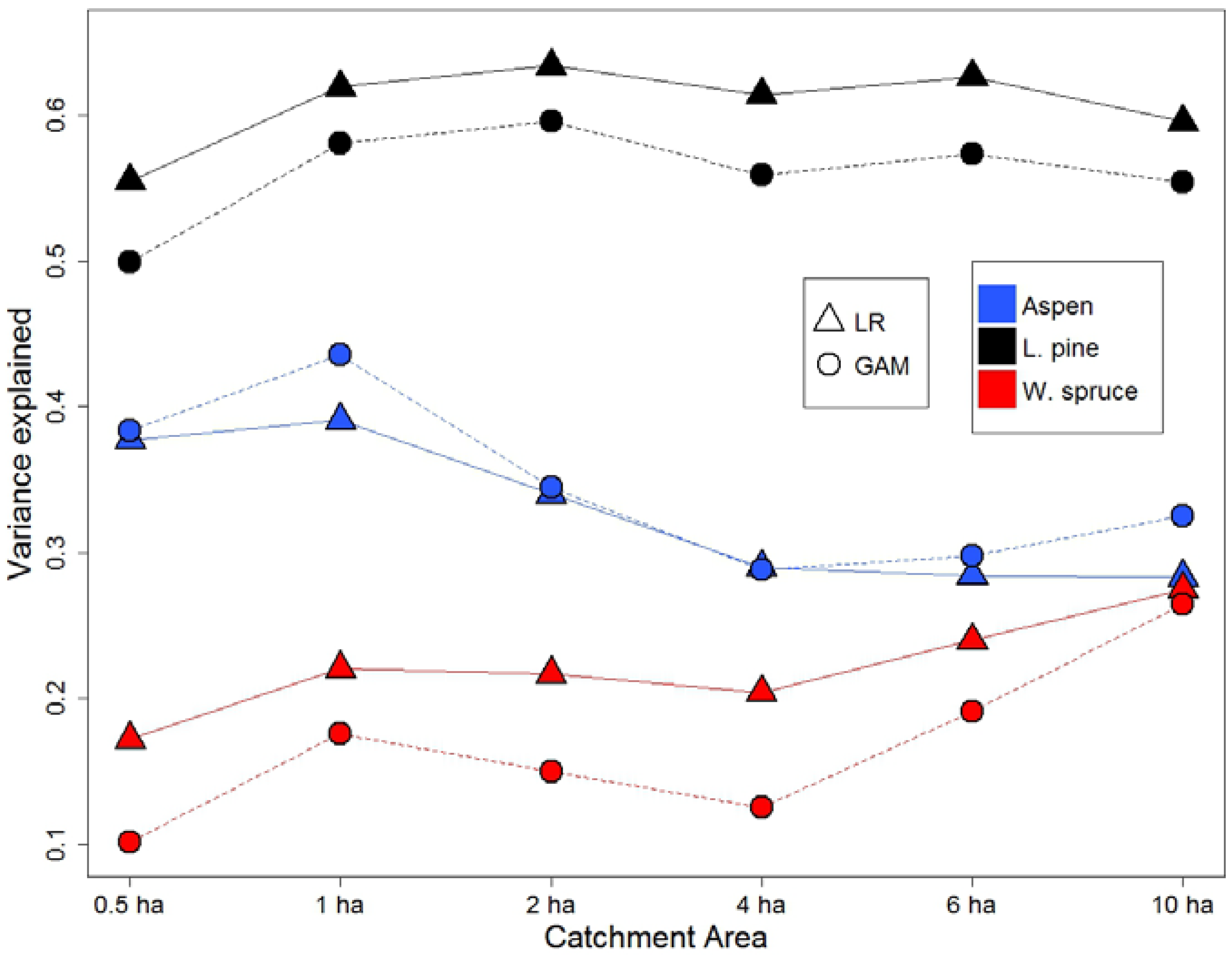
Figure 3.
Relationships between SI and selected DTW index fitted (A) LM (linear regression), and (B) GAM (generalized additive models). DTW is calculated at a CA of 1 ha for aspen, 2 ha for pine, and 10 ha for spruce. Note that on the x-axis DTW index is different for each species.
Figure 3.
Relationships between SI and selected DTW index fitted (A) LM (linear regression), and (B) GAM (generalized additive models). DTW is calculated at a CA of 1 ha for aspen, 2 ha for pine, and 10 ha for spruce. Note that on the x-axis DTW index is different for each species.
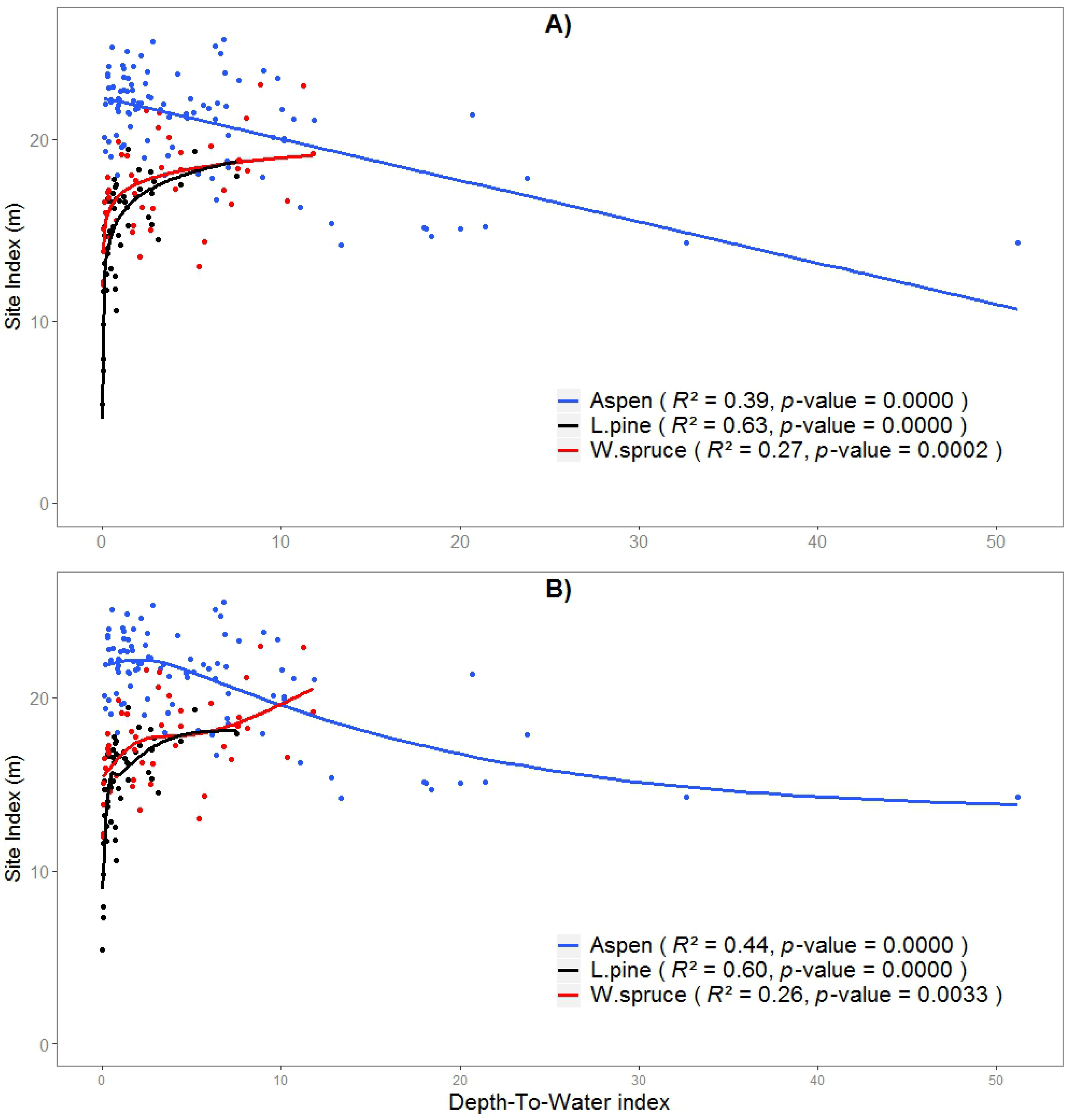
Figure 4.
Comparison of models between species, data sources (RS—remotely sensed, WAM—wet areas mapping; GB—ground survey-based) and modeling techniques based on the explained variance. Numbers represent the mean, and error bars represent the standard error of the mean.
Figure 4.
Comparison of models between species, data sources (RS—remotely sensed, WAM—wet areas mapping; GB—ground survey-based) and modeling techniques based on the explained variance. Numbers represent the mean, and error bars represent the standard error of the mean.

Figure 5.
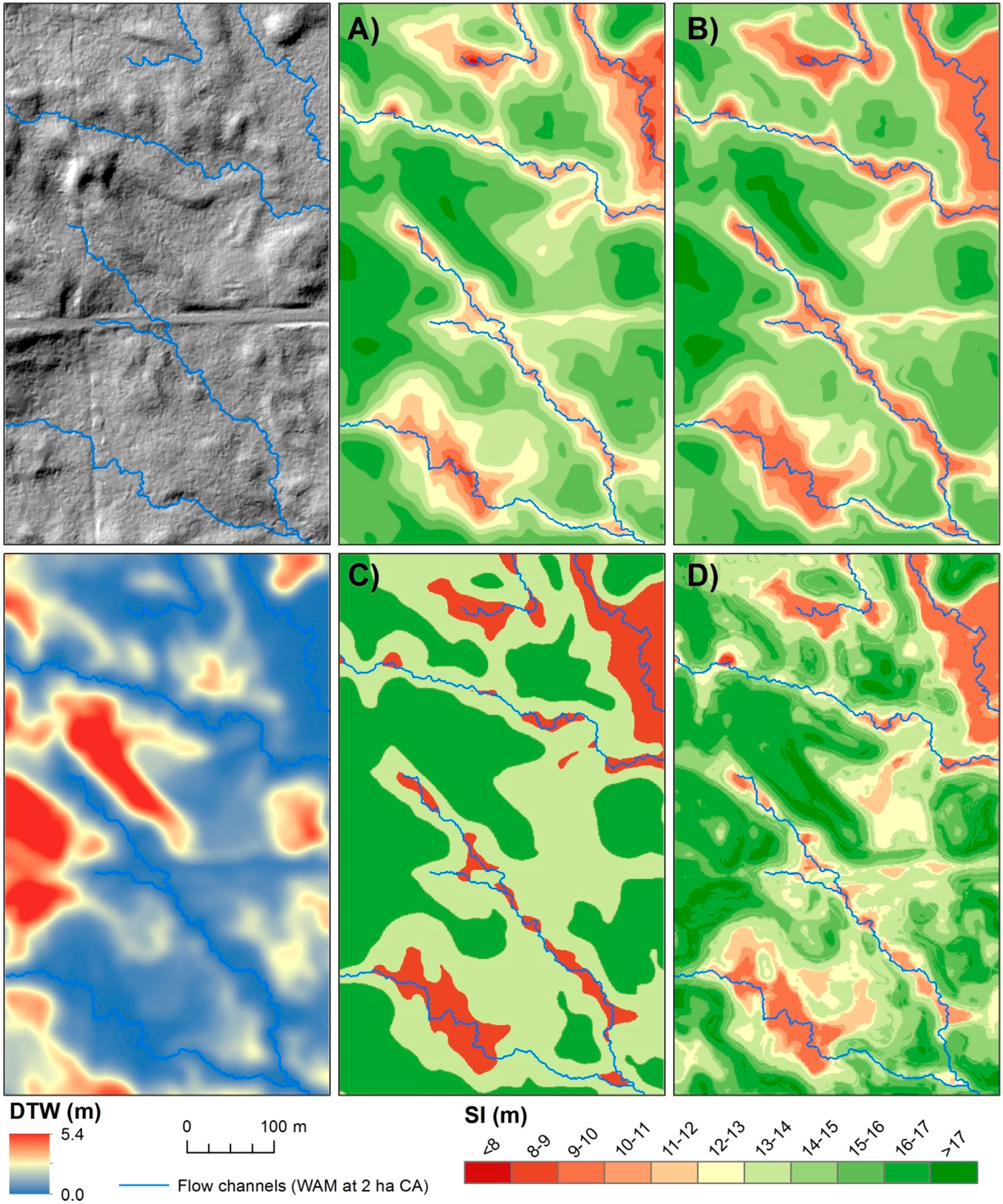
Hillshade (upper left), DTW (lower left), and mapped aspen SI generated based on the selected: (A) MLR model, (B) GAM model, (C) RT model, and (D) RF model. DTW and flow channels are computed at the 1 ha catchment area (CA). The map resolution is 1 m.
Figure 5.
Hillshade (upper left), DTW (lower left), and mapped aspen SI generated based on the selected: (A) MLR model, (B) GAM model, (C) RT model, and (D) RF model. DTW and flow channels are computed at the 1 ha catchment area (CA). The map resolution is 1 m.
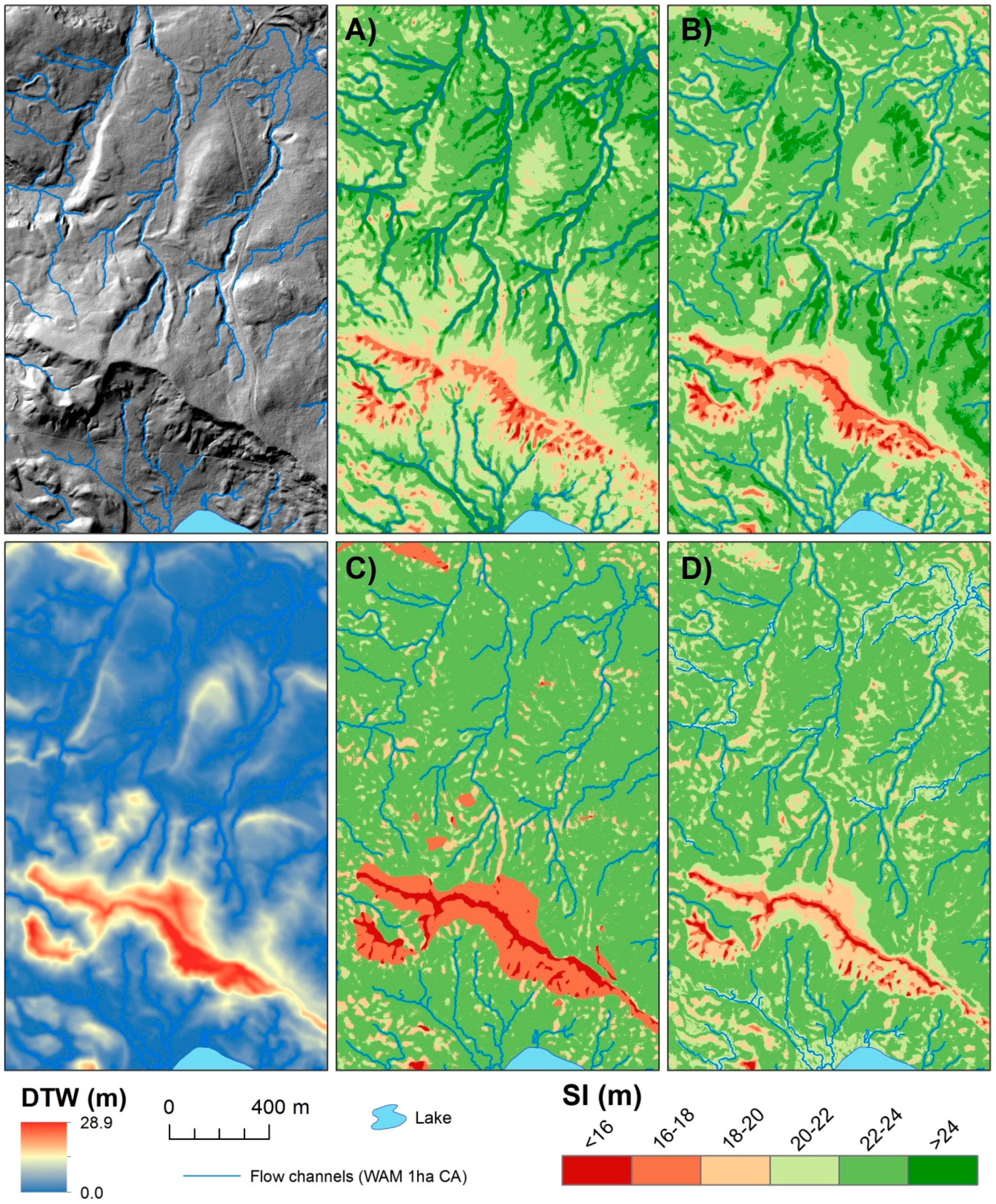
Figure 6.
Hillshade (upper left), DTW (lower left), and mapped white spruce SI generated based on the selected: (A) MLR model, (B) GAM model, (C) RT model, and (D) RF model. DTW and flow channels are computed at the 10 ha catchment area (CA). The map resolution is 1 m.
Figure 6.
Hillshade (upper left), DTW (lower left), and mapped white spruce SI generated based on the selected: (A) MLR model, (B) GAM model, (C) RT model, and (D) RF model. DTW and flow channels are computed at the 10 ha catchment area (CA). The map resolution is 1 m.
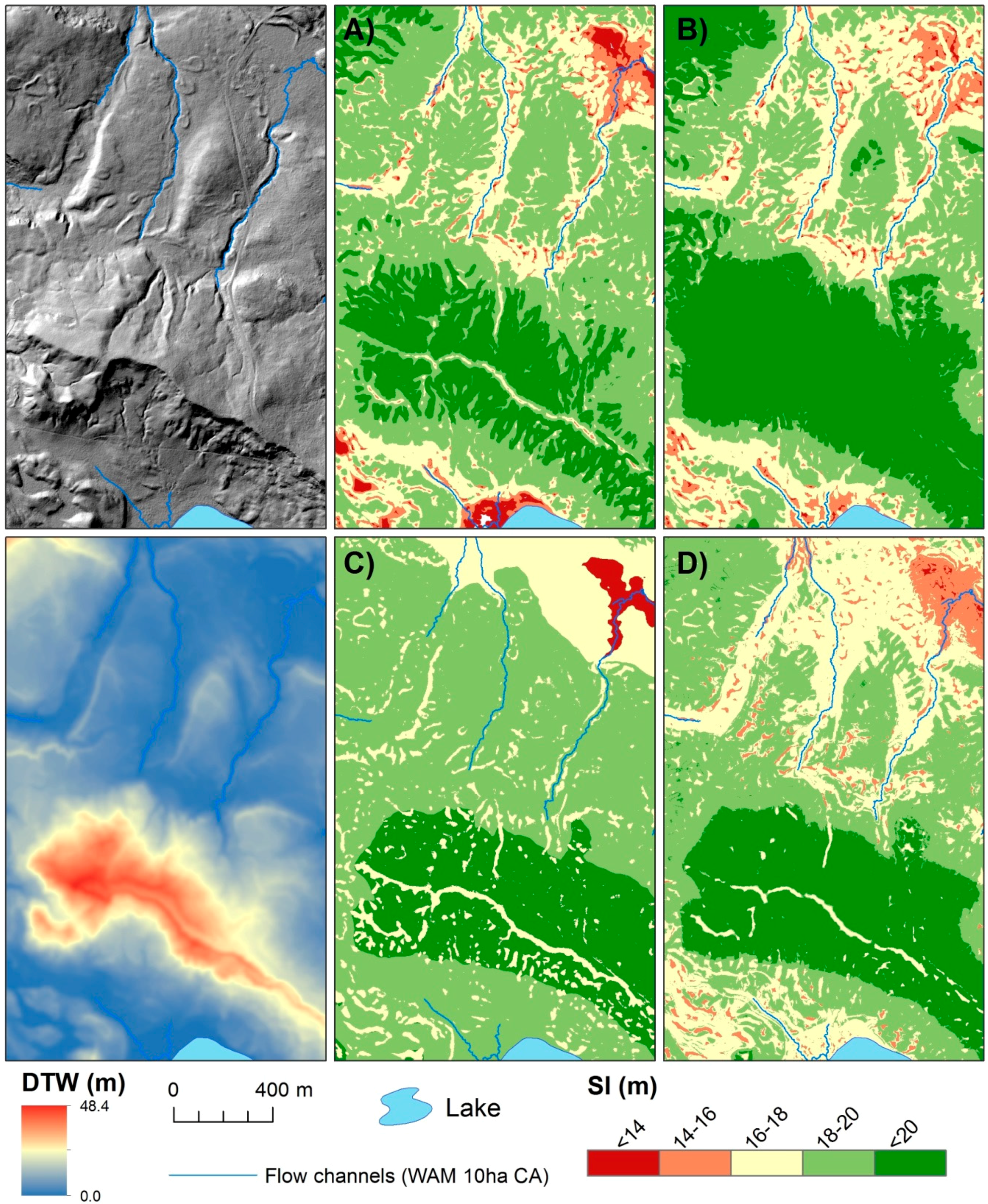
Figure 7.
Hillshade (upper left), DTW (lower left), and mapped lodgepole pine SI generated based on the selected: (A) MLR model, (B) GAM model, (C) RT model, and (D) RF model. DTW and flow channels are computed at the 2 ha catchment area (CA). The map resolution is 1 m.
Figure 7.
Hillshade (upper left), DTW (lower left), and mapped lodgepole pine SI generated based on the selected: (A) MLR model, (B) GAM model, (C) RT model, and (D) RF model. DTW and flow channels are computed at the 2 ha catchment area (CA). The map resolution is 1 m.

Table 1.
Descriptive statistics for variables used in analysis. Digital elevation model (DEM) and wet areas mapping (WAM) variables are derived from airborne LiDAR data. Ecological field surveys followed [28].
Table 1.
Descriptive statistics for variables used in analysis. Digital elevation model (DEM) and wet areas mapping (WAM) variables are derived from airborne LiDAR data. Ecological field surveys followed [28].
| Trembling Aspen (n = 97) | Lodgepole Pine (n = 50) | White Spruce (n = 45) | Trembling Aspen (n = 97) | Lodgepole Pine (n = 50) | White Spruce (n = 45) | ||||
|---|---|---|---|---|---|---|---|---|---|
| Variable | Abbrev. | Mean (S.D.) | Mean (S.D.) | Mean (S.D.) | Variable | Abbrev. | Mean (S.D.) | Mean (S.D.) | Mean (S.D.) |
| Map-based (remote sensing) variables | Field survey-based (ground-based) variables | ||||||||
| Depth-to-water at 0.5 ha CA (m) | DTW_0.5 | 4.51 (5.76) | 1.00 (1.13) | 1.97 (2.08) | Site Index (base 50 years) | SI | 20.97 (2.78) | 14.93 (3.02) | 17.40 (2.67) |
| Depth-to-water at 1 ha CA (m) | DTW_1 | 5.80 (7.65) | 1.14 (1.33) | 2.35 (2.47) | Soil organic thickness (cm) | SOT | 45.6 (0.7) | 43.4 (3.0) | 83.2 (13.8) |
| Depth-to-water at 2 ha CA (m) | DTW_2 | 7.47 (8.97) | 1.22 (1.47) | 2.67 (2.66) | Coarse fragments (%) | CF | 10.8 (5.3) | 11.8 (14.0) | 15.9 (10.7) |
| Depth-to-water at 4 ha CA (m) | DTW_4 | 10.01 (10.78) | 1.56 (1.85) | 2.82 (2.82) | Humus form | HUM | 7.1 (13.0) | 11.1 (15.2) | 5.4 (12.7) |
| Depth-to-water at 6 ha CA (m) | DTW_6 | 11.35 (11.92) | 1.86 (2.31) | 3.28 (3.29) | Texture | TEXT | 8.01 (1.96) | 7.92 (1.70) | 8.93 (1.60) |
| Depth-to-water at 10 ha CA (m) | DTW_10 | 12.68 (12.57) | 1.96 (2.37) | 3.51 (3.33) | Effective texture class | ETEXT | 3.69 (0.68) | 3.76 (0.59) | 3.82 (0.44) |
| Flow accumulation | FA | 15.7 * (169.1) | 12.3 * (393.2) | 42.7 * (21,994.9) | Drainage | DRN | 3.57 (0.90) | 3.58 (1.05) | 3.89 (1.13) |
| Altitude (m) | ALT | 810.9 (38.5) | 840.6 (42.9) | 802.3 (43.1) | Soil moisture regime | SMR | 4.97 (0.73) | 4.98 (0.94) | 5.44 (0.84) |
| Aspect index N-S folded | AI0 | 95.1 (37.5) | 96.7 (34.1) | 84.4 (41.5) | Soil nutrient regime | SNR | 3.14 (0.58) | 2.48 (0.58) | 3.47 (0.55) |
| Aspect index NE-SW folded | AI45 | 88.9 (40.2) | 86.0 (36.7) | 72.0 (40.1) | Altitude (m) | ALTT | 797.2 (38.2) | 824.5 (42.8) | 786.5 (43.5) |
| Slope (%) | SLO | 18.1 (13.5) | 4.5 (9.8) | 16.2 (9.0) | Aspect index N-S folded | AI0K | 96.5 (49.1) | 50.0 (104.0) | 92.2 (50.7) |
| Mean curvature | MCUR | 0.9 (1.64) | 0.64 (0.84) | 0.14 (1.25) | Aspect index NE-SW folded | AI45K | 86.1 (52.8) | 89.9 (53.7) | 80.3 (56.0) |
| Profile curvature | PRCUR | −0.59 (1.10) | −0.39 (0.46) | 0.06 (0.84) | Slope (%) | SLOV | 18.5 (17.6) | 9.6 (6.3) | 15.8 (11.9) |
| Plan curvature | PLCUR | 0.30 (0.68) | 0.25 (0.49) | 0.20 (0.79) | Slope Position | SPI | 4.12 (1.36) | 4.2 (1.48) | 3.47 (1.16) |
| Topographic Wetness Index | TWI | 70.1 * (2288.9) | 97.7 * (2704.8) | 69.5 * (529.5) | |||||
| Slope Position Index (15 m) | SPI15 | 3.90 (1.13) | 3.32 (1.25) | 3.51 (1.20) | |||||
| Slope Position Index (20 m) | SPI20 | 4.12 (1.33) | 3.38 (1.32) | 3.56 (1.29) | |||||
* Median; S.D.: standard deviation; CA: catchment area.
Table 2.
Variables included and model performance measures of selected models by species, data sources and modeling techniques. Abbreviations: RMSE—root mean squared error; rRMSE—normalized RMSE to the mean of measured data; Variance explained—R2 adjusted for the sample size and the number of variables included in the model; BIC—Bayesian information criteria. AIC—Akaike information criteria; RS—remotely sensed; GB—ground survey-based. Note: performance measures of Random Forest models were computed from cross-validation (OOB) samples.
| Species | Data Source | Mod. Method | No. Par. | Variables | RMSE (m) | rRMSE (%) | Variance Explained | AIC | BIC |
|---|---|---|---|---|---|---|---|---|---|
| Aspen | RS | MLR | 5 | DTW_1, FA, ALT, AI45, PLCUR | 1.63 | 7.77 | 0.64 | 104.8 | 117.7 |
| GAM | 4 | DTW_1, FA, AI45, SPI20 | 1.54 | 7.34 | 0.66 | 91.8 | 102.1 | ||
| RT | 5 | DTW_1, FA, ALT, SLO, PLCUR | 1.47 | 7.01 | 0.70 | 84.7 | 97.6 | ||
| RF | 3 | DTW_1, FA, SPI20 | 1.74 | 8.30 | 0.59 | 113.5 | 121.2 | ||
| WAM | MLR | 2 | DTW_1, FA | 1.91 | 9.11 | 0.51 | 129.5 | 134.7 | |
| GAM | 2 | DTW_1, FA | 1.70 | 8.11 | 0.60 | 106.9 | 112.1 | ||
| RT | 2 | DTW_1, FA | 1.55 | 7.39 | 0.68 | 89.0 | 94.2 | ||
| RF | 2 | DTW_1, FA | 1.82 | 8.68 | 0.56 | 120.2 | 125.3 | ||
| GB | MLR | 5 | SNR, ALTT, AI45K, SLOV, SP | 1.59 | 7.58 | 0.65 | 100.0 | 117.4 | |
| GAM | 5 | SNR, ALTT, AI45K, SLOV, SP | 1.59 | 7.58 | 0.65 | 100.0 | 112.8 | ||
| RT | 4 | ALTT, AI45K, SLOV, SP | 1.65 | 7.87 | 0.63 | 105.2 | 115.4 | ||
| RF | 4 | SMR, ALTT, SLOV, SP | 1.83 | 8.73 | 0.55 | 125.2 | 135.5 | ||
| L. pine | RS | MLR | 2 | DTW_2, ALT | 1.54 | 10.31 | 0.72 | 47.2 | 51.0 |
| GAM | 2 | DTW_2, ALT | 1.59 | 10.65 | 0.69 | 50.4 | 54.2 | ||
| RT | 2 | DTW_2, ALT | 1.52 | 10.18 | 0.73 | 45.9 | 49.7 | ||
| RF | 3 | DTW_2, ALT, SLO | 1.77 | 11.86 | 0.63 | 63.1 | 68.8 | ||
| WAM | MLR | 2 | DTW_2, FA | 1.73 | 11.59 | 0.65 | 58.8 | 62.6 | |
| GAM | 2 | DTW_2, FA | 1.80 | 12.06 | 0.60 | 62.8 | 66.6 | ||
| RT | 1 | DTW_2 | 1.77 | 11.86 | 0.65 | 59.1 | 64.9 | ||
| RF | 2 | DTW_2, FA | 2.26 | 15.14 | 0.42 | 85.5 | 89.4 | ||
| GB | MLR | 3 | SNR, ALTT, SP | 1.69 | 11.32 | 0.66 | 58.5 | 64.2 | |
| GAM | 3 | SNR, ALTT, SP | 1.68 | 11.25 | 0.66 | 57.9 | 63.6 | ||
| RT | 3 | SNR, ALTT, SP | 1.71 | 11.45 | 0.66 | 59.6 | 65.4 | ||
| RF | 4 | SNR, ALTT, SLOV, SP | 1.73 | 11.59 | 0.64 | 62.8 | 70.5 | ||
| W. spruce | RS | MLR | 2 | DTW_10, FA | 2.01 | 11.55 | 0.39 | 66.8 | 70.4 |
| GAM | 2 | DTW_10, FA | 2.06 | 11.84 | 0.34 | 69.0 | 72.7 | ||
| RT | 3 | DTW_10, ALT, SPI20 | 1.91 | 10.98 | 0.44 | 64.2 | 69.7 | ||
| RF | 3 | DTW_10, FA, ALT | 2.14 | 12.30 | 0.31 | 74.5 | 79.9 | ||
| WAM | MLR | 2 | DTW_10, FA | 2.01 | 11.55 | 0.39 | 66.8 | 70.4 | |
| GAM | 2 | DTW_10, FA | 2.06 | 11.84 | 0.34 | 69.0 | 72.6 | ||
| RT | 2 | DTW_10, FA | 1.90 | 10.92 | 0.47 | 61.8 | 65.4 | ||
| RF | 2 | DTW_10, FA | 2.33 | 13.39 | 0.20 | 80.1 | 83.7 | ||
| GB | MLR | 2 | HUM, DRN | 1.84 | 10.57 | 0.49 | 58.9 | 62.5 | |
| GAM | 2 | HUM, DRN | 1.82 | 10.46 | 0.50 | 57.9 | 61.5 | ||
| RT | 2 | HUM, DRN | 1.91 | 10.98 | 0.46 | 62.2 | 65.9 | ||
| RF | 2 | HUM, DRN | 2.03 | 11.67 | 0.39 | 67.7 | 71.3 |
© 2018 by the authors. Licensee MDPI, Basel, Switzerland. This article is an open access article distributed under the terms and conditions of the Creative Commons Attribution (CC BY) license (http://creativecommons.org/licenses/by/4.0/).
Share and Cite
MDPI and ACS Style
Bjelanovic, I.; Comeau, P.G.; White, B. High Resolution Site Index Prediction in Boreal Forests Using Topographic and Wet Areas Mapping Attributes. Forests 2018, 9, 113. https://doi.org/10.3390/f9030113
AMA Style
Bjelanovic I, Comeau PG, White B. High Resolution Site Index Prediction in Boreal Forests Using Topographic and Wet Areas Mapping Attributes. Forests. 2018; 9(3):113. https://doi.org/10.3390/f9030113
Chicago/Turabian StyleBjelanovic, Ivan, Philip G. Comeau, and Barry White. 2018. "High Resolution Site Index Prediction in Boreal Forests Using Topographic and Wet Areas Mapping Attributes" Forests 9, no. 3: 113. https://doi.org/10.3390/f9030113
Note that from the first issue of 2016, this journal uses article numbers instead of page numbers. See further details here.