Optimizing Biomass Feedstock Logistics for Forest Residue Processing and Transportation on a Tree-Shaped Road Network


1
Department of Forest Engineering, Resources and Management, College of Forestry, Oregon State University, Corvallis, OR 97331, USA
2
Division of Forest Industry Research, National Institute of Forest Science, Seoul 02455, Korea
3
Rocky Mountain Research Station, USDA Forest Service, Missoula, MT 59807, USA
*
Author to whom correspondence should be addressed.
Forests 2018, 9(3), 121; https://doi.org/10.3390/f9030121
Submission received: 26 January 2018
/
Revised: 23 February 2018
/
Accepted: 2 March 2018
/
Published: 5 March 2018
(This article belongs to the Section Forest Ecology and Management)
Abstract
:An important task in forest residue recovery operations is to select the most cost-efficient feedstock logistics system for a given distribution of residue piles, road access, and available machinery. Notable considerations include inaccessibility of treatment units to large chip vans and frequent, long-distance mobilization of forestry equipment required to process dispersed residues. In this study, we present optimized biomass feedstock logistics on a tree-shaped road network that take into account the following options: (1) grinding residues at the site of treatment and forwarding ground residues either directly to bioenergy facility or to a concentration yard where they are transshipped to large chip vans, (2) forwarding residues to a concentration yard where they are stored and ground directly into chip vans, and (3) forwarding residues to a nearby grinder location and forwarding the ground materials. A mixed-integer programming model coupled with a network algorithm was developed to solve the problem. The model was applied to recovery operations on a study site in Colorado, USA, and the optimal solution reduced the cost of logistics up to 11% compared to the conventional system. This is an important result because this cost reduction propagates downstream through the biomass supply chain, reducing production costs for bioenergy and bioproducts.
1. Introduction
Forest biomass represents one of the major renewable raw materials for bioenergy and bioproducts. Approximately 42% of currently used biomass resources in the United States are from forestlands, accounting for 154 million dry tons (short ton, US) of biomass annually. It is estimated that at a price of $60 per dry ton an additional 103 million dry tons of forest biomass is potentially available annually [1]. In the European Union, it is estimated the total forest biomass supply could increase to 895 million m3 per year by 2030, which is 20% higher than its supply level in 2010 [2]. In Brazil, Welfle [3] evaluated the country’s potential biomass supply from forest residues and estimated the supply could increase to approximately 16 million tons in 2030, 3.6 times larger than the supply in 2015. Although there has been a growing interest in utilizing forest biomass, many factors still constrain the development of viable markets for forest biomass. One significant barrier is the high costs of feedstock logistics coupled with low marginal value.
Forest biomass feedstock logistics has been a subject of intense investigation for more than a decade in many different regions due to the interest in improving the economic viability of forest biomass utilization [4]. Some of this research has been focused directly on the processing and transportation of biomass residues from timber harvest, fuel thinning, and forest restoration activities. For example, Harrill and Han [5] evaluated the operational performance and costs of utilizing a hook-lift truck in centralized grinding operations in northern California. They found the hook-lift truck transportation was cost-effective in collecting previously inaccessible forest residues with the production cost at $32.98 per bone dry ton. Zamora-Cristales et al. [6] analyzed the economic effects of truck-grinder interference and found grinder location, available truck turnaround, turnouts and truck travel distance highly affect forest residues processing and transport economics at the operational level. Marchi et al. [7] compared two chipping operations in Italy and found that a roadside chipping was over 4 times more productive than chipping in the forest stand.
Biomass feedstock logistics include preprocessing, storage and transportation to an end-use facility [8,9]. On-site preprocessing, such as grinding or chipping, is usually required to improve transportation efficiency and meet desired particle size specifications for energy and product conversion processes. In many situations, however, preprocessing is responsible for a substantial portion of feedstock costs because of high machine rates (owning and operating costs) combined with low machine utilization rates due to frequent equipment relocation between processing sites [10]. In addition, efficiency gains in transportation from densifying materials through preprocessing can become inconsequential if poor road conditions impede large chip vans from accessing the site and dramatically increase per-unit transportation costs [11]. Careful selection of equipment and design of efficient feedstock logistics are essential considerations for economically feasible forest biomass supply.
At their core, decisions related to grinder location are fundamentally connected to the tradeoffs between fixed and variable costs in residue processing and trucking operations. For a single pile, a simple tradeoff equation can be developed and solved for volume or distance, and many operators use conventional wisdom and simple rules of thumb to site equipment for biomass operations. However, real-world operations can be quite complex and the design of efficient biomass supply logistics involves multiple decisions that are simultaneously sensitive to numerous parameters, such as the spatial distribution and quantity of biomass sources, road infrastructure and conditions, available equipment, storage and conversion facility locations, and many other variables. Optimization techniques have been used in the past to assist forest biomass supply decisions but mostly at strategic or tactical scales [12]. Some of the applications include selection of biomass facility location [13], selection of conversion technology and energy products [14], biomass procurement and supply management [15], production planning of biomass power plants [16], chipping facility location and transportation [17], and truck scheduling for biomass delivery [18].
Although these studies suggest effective solution approaches to broad forest biomass supply chain problems, many did not incorporate operational details related to feedstock logistics into their optimization frameworks. Generally, timber harvests and other silvicultural treatments that are responsible for producing residues are spatially dispersed, as they often must comply with maximum adjacency, size and green-up constraints. As a result, forest residues are geographically dispersed, which is a reality seldom considered by large-scale, strategic planning models. Furthermore, the use of certain truck configurations may be limited by changes in road conditions that occur at spatial resolutions that are finer than those used by course strategic models. Individual machines must be selected for tasks and site-specific conditions and the entire system should be carefully designed to minimize negative interactions and operational delays among machines to maximize system productivity.
Zamora-Cristales et al. [10] is one of few studies that incorporated operational details into an optimization framework for forest biomass feedstock production. The study used simulation techniques to quantify the effects of truck-machine interactions, truck arrival rates and road conditions. The study then solved feedstock logistics problems using a mixed-integer programming approach to select the most cost-efficient biomass processing and transportation decisions at an operational level. The study took into account different transportation configurations, and comminution and densification options to provide an optimal combination of machines and operations for individual residue piles. This approach, however, assumes that multiple machines are available to the contractor at all times. Small forest contracting firms generally own a small fleet of machines, perhaps only one machine per task (e.g., one feller-buncher, one skidder, one delimber), and their short-term goal is often to make the best use of their existing and available machines through improved logistics solutions for a fixed portfolio of equipment.
Anderson et al. [11] conducted field operations studies to explore two different logistics systems for forest biomass processing and transportation where residue sites were inaccessible to large chip vans. They compared “in-woods grinding” and “slash forwarding”, and analyzed tradeoffs in grinder and truck efficiencies between the two systems. In the conventional in-woods grinding system, the grinder moves to each of the forest residue piles and grinds them on the site. A maneuverable, small capacity dump truck is used to transport the ground material to a concentration yard (also called a “transshipment” location) where it is stored and eventually reloaded into large chip vans for long-distance highway transportation to a conversion facility. In contrast, slash forwarding uses a dump truck to forward residues to a concentration yard where the residues are ground directly into large chip vans. Anderson et al. [11] found that processing costs were higher for in-woods grinding due to the low utilization rate of the grinder compared to slash forwarding. However, truck efficiency was higher for in-woods grinding because wood chips have a higher bulk density than unprocessed residues.
While Anderson et al. [11] showed tradeoffs between grinder and truck efficiencies, the measured tradeoffs are only pertinent to their experiments and may not be applicable to other operational conditions. Furthermore, the research used high-resolution time study methods, but did not employ engineering approaches to optimize logistics. In this study, we developed a mixed-integer programming model that optimizes feedstock logistics on a tree-shaped road network by minimizing total feedstock processing and handling costs. Similar to Anderson et al. [11], our model evaluates tradeoffs between slash forwarding and in-woods grinding operations, but it provides optimal configurations for equipment selection, processing and transportation for any given machine productivity and costs, potential concentration yard locations and road network. For demonstration purposes, our model was applied to different sets of residue piles dispersed across a road network in the Uncompahgre National Forest in southwestern Colorado.
2. Problem Description
An obvious advantage of the in-woods grinding system (Figure 1a) is increased transportation efficiency compared to slash forwarding, in which gains in transportation efficiency attributable to biomass densification are only realized after sufficiently dry residues have been ground at the concentration yard. It is clear that this system is increasingly more attractive than slash forwarding, in terms of transport efficiency, as the distance between the grinding site and the conversion facility increases. However, even though slash is much less dense than chipped or ground residues, move-in and move-out costs of walking or trucking the grinder to the residue pile location and its low utilization rate due to frequent relocation and unproductive wait time for trucks can make in-woods grinding economically inefficient compared to slash forwarding. Moreover, reloading the ground materials into large chip vans at the concentration yard involves additional handling costs.
In situations where in-woods grinding becomes inefficient, slash forwarding to the concentration yard using small dump trucks presents a potentially more efficient alternative recovery operation (Figure 1b). In this configuration, the grinder is not operationally constrained by the productivity of small trucks delivering slash because a sufficient volume of residues can be stored at the concentration yard, thus maximizing grinder efficiency. However, the high cost of transporting slash residues by small dump trucks may offset reduced grinding costs if forwarding of the raw material is carried out over long distances [11].
Another system combines these two options, including both slash forwarding and in-woods grinding components. Instead of forwarding slash directly to the concentration yard, slash from a given site can be advanced to a nearby site where it is processed and transported to the concentration yard (Figure 1c). Rather than moving the grinder between piles, the grinder stays at one pile site, or a location on the road network central to a set of surrounding piles (hereafter called a “grinder depot”), and processes residues as they are forwarded from nearby sites. In certain situations, this option would minimize grinder mobilization and increase transportation efficiency simultaneously. However, it clearly adds an additional handling step and potentially a second loader, depending on how the logistics are timed.
Forest contractors involved in forest residue processing and handling operations need to select the most cost-efficient feedstock logistics system for a given distribution of residue pile sites, road access, and available machinery. We developed a mathematical model that can be used to: (1) inform the contractor of the best allocation of in-woods grinding and slash forwarding operations, (2) facilitate the decision to construct (or not to construct) a concentration yard, and (3) guide the minimal relocation of equipment to minimize overall costs.
3. Model Development
Our model consists of three components: user data entry, network modeling and problem solving (Figure 2). The model was designed to work with any user-specific data on machine costs and productivity because individual logging contractors may have different fleets of machines with different capacities and costs. Non-spatial, user-specific data include the capacity, hourly costs and productivity of individual machines, fixed and variable costs of equipment mobilization when a lowboy is used and driving speed when the equipment is self-propelled without using a lowboy, and feedstock processing site construction costs. Another required user-specific dataset is spatial road network data in vector format consisting of nodes and links including road segment attributes, logging residue pile locations, potential concentration yard locations, road junctions, and a conversion facility location.
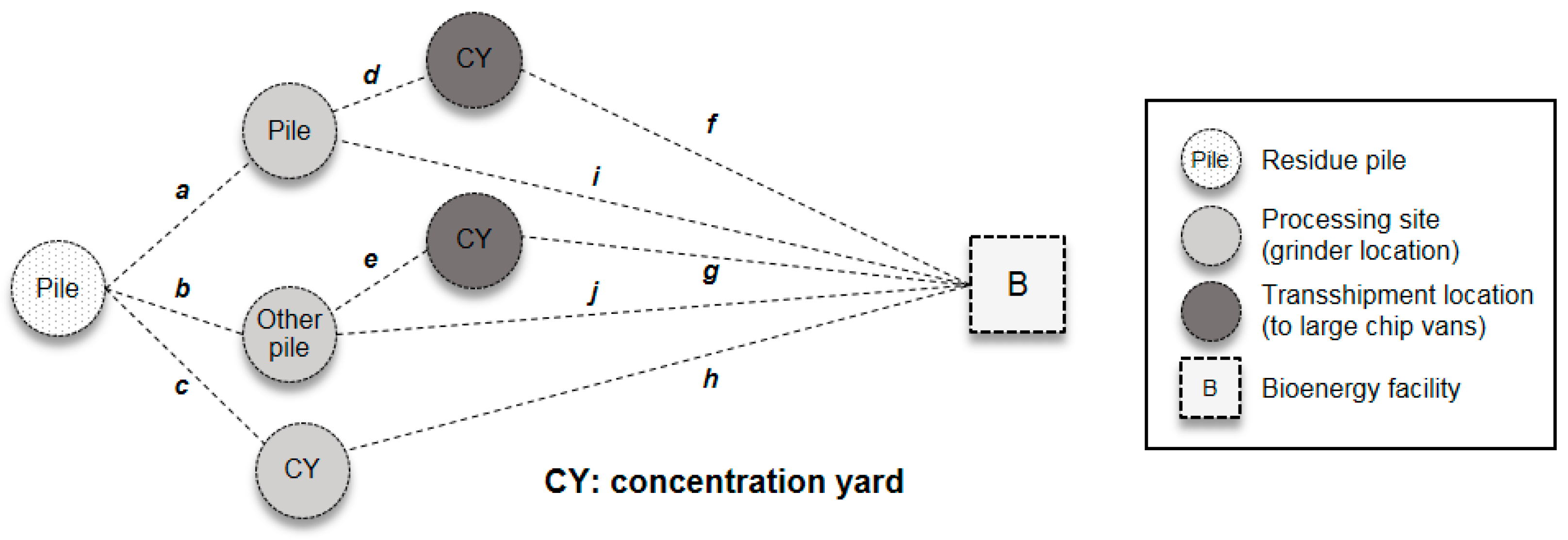
After the user-specific tabular and spatial data are entered, the model builds a network representation of the problem to accommodate the different operational configurations (Figure 3). For the in-woods grinding option, the residues could be either processed at their current location, link a in Figure 3, if the landing serves as a processing site, or processed at another landing location, link b, after forwarding the slash. The ground materials are then transported to a nearby concentration yard using dump trucks, links d and e, or directly to the bioenergy facility through links i and j, whichever is the lowest cost option. The ground materials delivered and stored at a concentration yard are reloaded into large chip vans and transported to the final destination via links f and g. For the slash forwarding system, the residue is forwarded to the concentration yard, link c, and then processed and transported to the bioenergy facility through link h. Different truck configurations and variable haul costs are used to represent truck transportation options, and the construction of processing sites is considered a fixed cost.
Our model takes user-provided spatial road network data, and uses Dijkstra’s shortest path algorithm [19] to build a network representation of the problem. Any given road network (G) may include a large number of nodes (N) and links (L). In our model, a subset network, G’= (N’, L’), is developed consisting of a set of nodes, N’, and a set of directed links L’. N’ represents “significant” nodes for biomass feedstock logistics including residue piles, concentration yards, bioenergy facilities, or any major intermediate nodes (i.e., road junctions), while L’ represents transportation options between a pair of any significant nodes with different truck options. The model runs the shortest path algorithm on the entire road network (G) to calculate the least-cost routes for the possible pairs of the preselected significant nodes (N’). These least-cost routes are then converted to a set of links (L’) directly linking the preselected significant nodes via different truck options. Costs for each transportation option are also calculated by the shortest path algorithm on a dry weight basis with units of bone dry tons (bdt, 907.185 kilograms at 0% water content). Running the shortest path algorithm prior to the mixed-integer formulation significantly reduces problem size because it predetermines the least-cost routes between significant nodes, and thus removes unnecessary intermediate nodes for a simpler network representation of the problem.
The model then builds a mixed-integer programming (MIP) formulation for the cost minimization network flow problem. The sets, decision variables, and parameters used in the MIP formulation are given in Table 1.
The mathematical formulation of the problem is as follows:
Subject to:
for
for
for
for
for ,
for ,
for
for
for
for
for
for
Equation (1) specifies the objective function of the problem: to minimize the total cost of the operation including grinding, transportation, residue loading, machine mobilization, and processing site construction. The first and second terms represent the costs of slash forwarding to processing sites (i.e., grinder depots and concentration yards shown as links a, b and c in Figure 3). The third term represents the costs of in-woods grinding along with the transportation costs of ground residues from processing sites to either a concentration yard (links d and e) or a bioenergy facility (links i and j). The fourth term estimates both grinding costs at a concentration yard and transportation costs of the ground materials to the bioenergy facility (link h). The fifth term estimates the transshipment and transportation costs of ground materials (links f and g). The sixth and seventh terms of the objective function represent the fixed costs of machine mobilization and processing site construction costs, respectively.
Equations (2)–(13) represent the constraints of the cost minimization problem. Equation (2) ensures the maximum available slash residues from each source node. Equation (3) provides the option of slash forwarding to a grinder depot, and ensures that ground materials can be only transported to a concentration yard for transshipment or directly to the bioenergy facility. When a residue plie location serves as a grinder depot, the slash flow variable from the location to itself has a positive value (i.e., Sii > 0). Equation (4) ensures all the slash materials arriving at the concentration yard are ground at the yard and transported to the bioenergy facility as ground residues. Equation (5) ensures all the ground materials forwarded to the concentration yard are transshipped to large chip vans for transportation to the bioenergy facility. Equations (6)–(9) trigger the use of machine m at node u required for slash forwarding (Equation (6)), residue grinding at the grinder depot (Equation (7)), residue grinding at the concentration yard (Equation (8)), or transshipment of ground materials at the concentration yard (Equation (9)). M is a large number greater than the minimum required delivered volume.
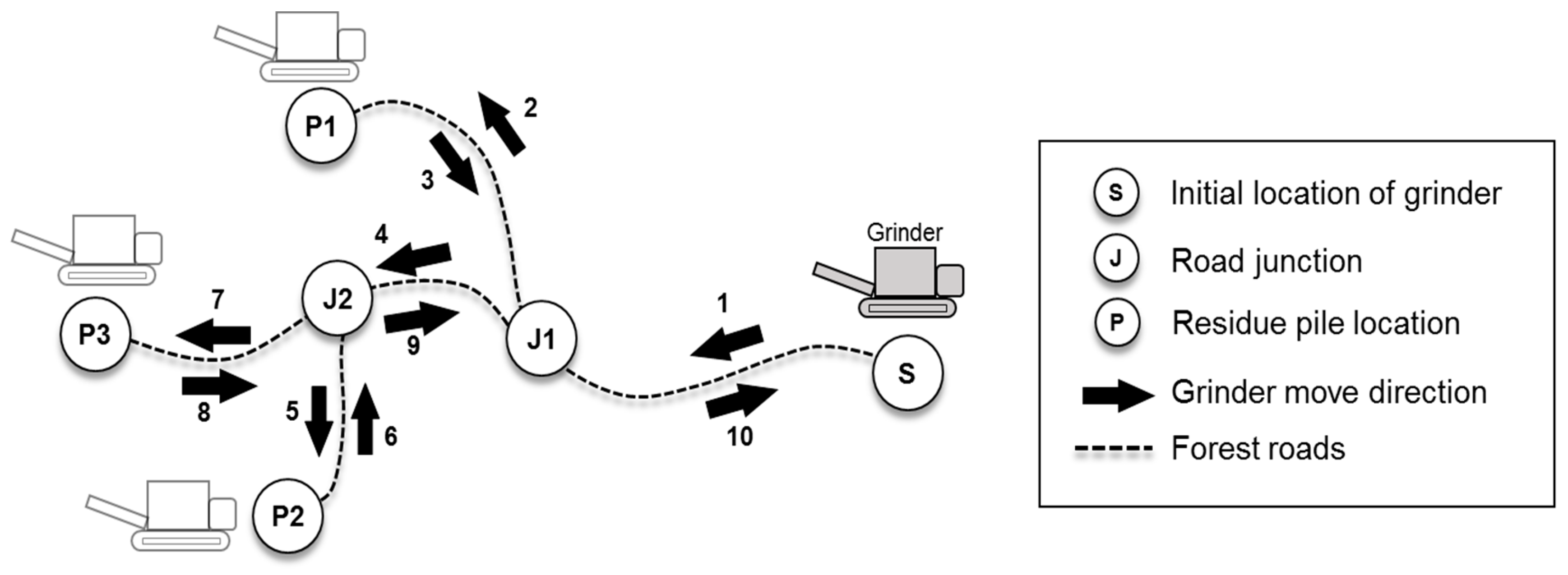
While Equations (1)–(9) are the typical MIP formulation for a network problem, Equation (10) shows the unique formulation approach developed in this study in order to model equipment mobilization between nodes in a hierarchical, tree-shaped network where equipment has to move out to the junction of the main road that connects to the final destination before it can move to another location. Consider the grinder mobilization tour illustrated in Figure 4. Under any circumstance, this tour would be accomplished by the round-trip travel of a machine over each road segment to move from the initial location to each pile (i.e., S-P1, P1-P2, and P2-P3). Thus, the machine mobilization cost can be calculated by multiplying the move-in costs of the machine by the road segments used for relocation (Equation (1)). Assuming the machine starts at the facility location (v), Equation (10) ensures that all of the links included in the shortest path (Ruv) between nodes u and v must be used if a machine m is located at the node u. This equation also ensures the model does not count the previously incurred mobilization expenses multiple times when the machine makes several stops along the route. For example, processing at P1 in Figure 4 requires that the grinder passes through road segments S-J1 and J1-P1. When the grinder visits P2 following processing at P1, the model adds the travel costs from J1 to P2 to the incurred expenses, but ignores the costs previously incurred between S and J1. This prevents the model from double counting mobilization costs.
Equation (11) represents the required minimum volume constraint for the demand of ground residues set by the bioenergy facility. The volume requirement at each biomass facility has to be fulfilled by the total amount of ground residues transported to the facility with all possible transportation options. It is not necessary to specify truck options in the formulation because material types (i.e., slash vs. ground residues) and truck options (i.e., dump truck vs. chip van) are specified by decision variables. For example, Sij represents slash forwarding by dump truck, which is the only option of transportation for slash residue. Gij represents ground residue transportation by dump truck, except when i is one of the concentration yards and j is the bioenergy facility, in which case it represents chip van transportation. Equation (12) shows the binary variables associated with machine mobilization and site construction. Equation (13) is a non-negativity constraint for continuous decision variables to guarantee that all the flows must be equal or greater than zero. All solutions presented hereafter were provided by CPLEX® Version 12.6 (IBM ILOG, Armonk, NY, USA) [20].
4. Model Application
4.1. Study Site and Analysis
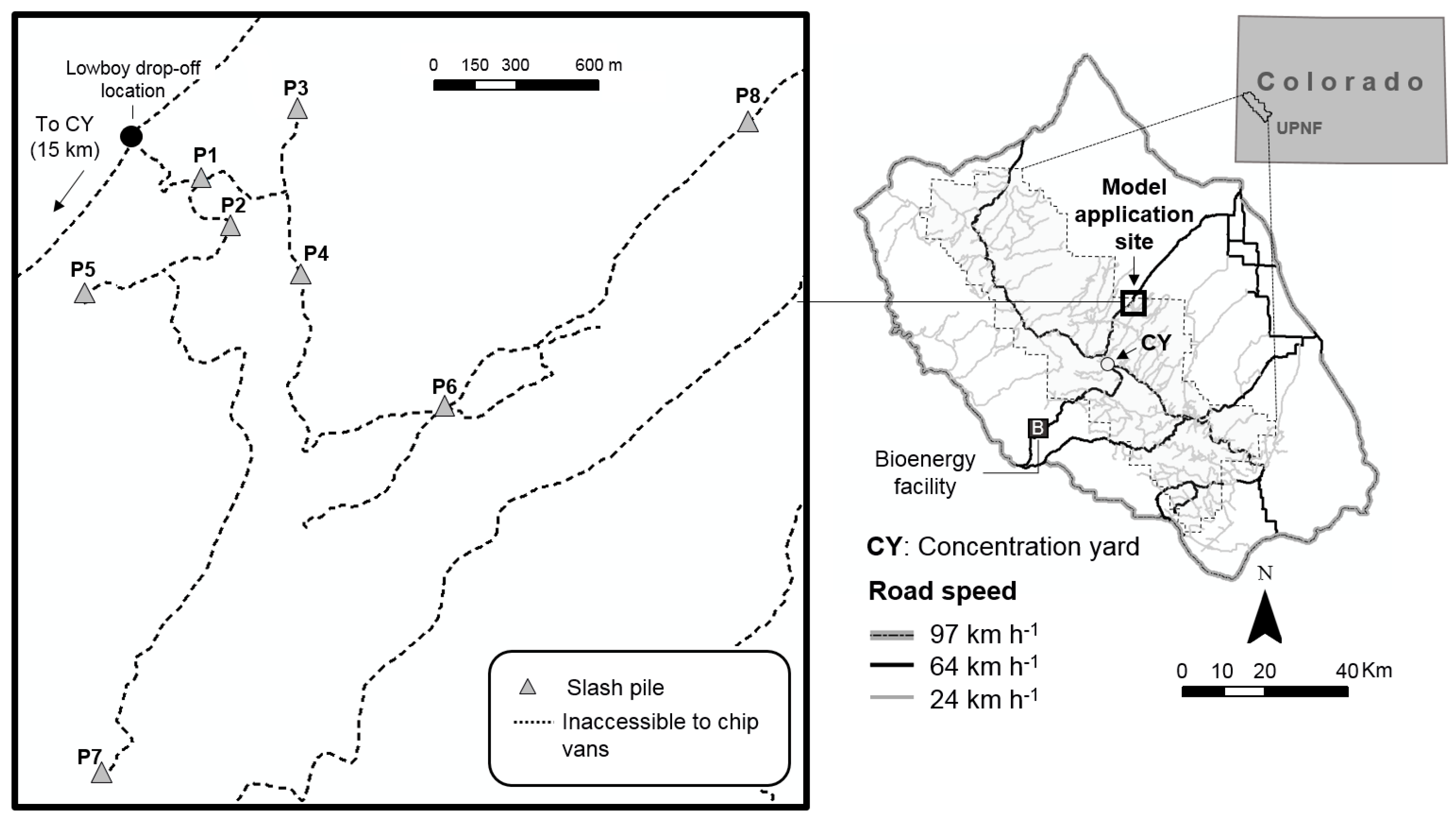
To demonstrate the use and applicability of the mathematical model in real-world biomass feedstock logistics, we applied the model to a small region of the Uncompahgre National Forest (UNF) in Colorado, USA (38°31′40” N, 108°18′54” W). Treatment residue volumes were estimated according to Wells et al. [21], considering site-specific silvicultural treatments and current stand conditions to predict residue volumes and location. We selected a subset of the road network on the UNF inaccessible to large chip vans (Figure 5). The concentration yard location was selected 15 km away from the site for chip van accessibility and sufficient space for residue processing and storing. A total of 1138 bdt of forest residue piles were available from 8 log landings (Table 2). Residue extraction was assumed to take place after timber harvesting and residue was allowed time to dry to a moisture content lower than 30% wet basis [21]. Each landing was considered eligible for on-site grinding and it was assumed that the grinder walks to the piles from the drop-off location if needed, where it can be delivered on a drop-deck semi-trailer (i.e., “lowboy”). The road network includes segments that connect individual log landings and intermediate nodes to the final bioenergy facility located approximately 36 km southwest of the concentration yard, in Nucla, Colorado. This site is the location of a 100 MW coal-fired power plant that recently considered co-firing biomass with coal [22]. This network problem consists of 25 road segments and 26 nodes including 8 pile locations and one final destination.
Conventional and optimized feedstock logistics were compared and tradeoffs between the two systems were analyzed. We assumed the grinder visits each pile location for processing in the conventional system. For the optimized logistics we considered both in-woods grinding and slash forwarding options, while taking into account a small fleet of machines: one grinder, two grapple loaders, and one front-end loader. As noted previously, this approach fits well with the type of forest contractor operating in the region rather than assuming an operator has a large and diverse fleet of equipment available for deployment. Based on the user data inputs, the model analyzes the best fit of machines to select the most cost-efficient logistics for given tasks and site conditions. We then explored the effects of biomass volume on the optimal solution by increasing and decreasing the volume at each residue pile site and developed associated strategies to inform the best use of machines under different volume assumptions. We also examined different biomass volume constraints to analyze how the volume constraints affect residue pile selection, the optimal feedstock logistics and costs. Lastly, we applied the model to a larger project area to demonstrate its utility in larger, landscape-scale biomass recovery operations. This large-size data set includes 222 road segments and 223 nodes with 58 pile locations. A desktop computer equipped with a 3.30 GHz Intel Core i5 processor and 16.0 Gbytes RAM was used to run the MIP model for all cases.
4.2. Equipment and Cost Calculations
The type of equipment, productivities, and truck capacities used in the model were adapted from [11] but equipment costs were updated based on machine prices and wage rates in the study region for 2016 (Table 3). Although the study by Anderson et al. [11] was conducted in Idaho, similar equipment is common and available in Colorado [23]. Ownership and operating costs were estimated using STHARVEST [24]. Machine prices were determined by regional market prices and a wage rate of $28.18 per scheduled machine hour (SMH), including fringe benefits, for logging equipment operators and truck drivers was used to estimate labor costs for each machine [25]. The lifespans of machines were assumed to be 10 years for trucks, 7 years for loaders, and 4 years for a grinder with a salvage value of 25%. Base utilization rate was set at 85% for the normal use of the grinder without frequent mobilization, and 90% for all the other equipment based on 2000 SMH year−1. The ownership costs were estimated with a 10% interest rate and 4% insurance rate on a yearly investment. The average off-road diesel price of $2.26 gallon−1 in the region was used to calculate fuel costs depending on fuel consumption rates determined by equipment horsepower. Additional assumptions for operating costs include repair and maintenance at 100% of depreciation, and lubrication at 40% of fuel cost.
Based on observations and calculations in previous operations studies, different costs for the grinder were used for processing at the concentration yard and on-site grinding, with rates for the two types of sites calculated by dividing the machine cost by the expected productivities at each location. Loading cost to fill trucks was considered when the loader is used for slash forwarding or reloading ground materials. The cost of the grapple loader used to feed the grinder was included in the grinder processing costs because these machines function as a unit.
Transportation costs were calculated considering the least-cost route based on engineered road speed, truck capacity, and loading and unloading time (Equation (14)). A total time required for loading and unloading was estimated according to cycle time values measured by Anderson et al. [11]: 1 h for loading ground material in chip vans, 0.16 h for dump trucks when loading slash residue, and 0.25 h for dump trucks when loading ground material (loading ground material consists of grinding slash directly into trucks). Transportation cost, including loading and unloading, was calculated as:
where tc is the transportation cost per bone dry ton ($ bdt−1), r is an hourly trucking cost ($ h−1), p is a truck capacity (bdt), is a round-trip travel time in hours over the least-cost route, and lu is loading and unloading time in hours.
Machine mobilization costs were considered for three machines: grinder, grapple loader, and front-end loader. The grinder and grapple loader are transported to the drop-off location using a lowboy trailer and it was assumed that these machines “walk” to pile locations where on-site grinding operation is needed. The front-end loader is also transported using a lowboy trailer but it stays at the concentration yard and is used for reloading ground materials into chip vans. Equation (15) was used for calculating mobilization cost with lowboy over a set of road segments following the approach presented in Bruce et al. [26]:
where,
where mct is the round-trip mobilization cost ($) of equipment to the lowboy drop-off location, f and v are the fixed and variable move-in costs, b is a backhaul charge for the return trip of the lowboy, c is an hourly lowboy cost ($ h−1), eown is the transported equipment ownership cost ($ h−1), lu is loading and unloading time, t1 is loaded travel time, and t2 is empty travel time of the lowboy.
The hourly lowboy cost including labor of operator was assumed at $100 h−1 as used in Zamora-Cristales [27]. Travel speeds of the lowboy and other equipment applied in the model are shown in Table 4. The mobilization cost of equipment walking to a processing site was calculated as follows:
where mcw is the round-trip mobilization cost ($) of a machine walking to piles, eown is the hourly equipment ownership cost ($ h−1), eop is the hourly equipment operating cost ($ h−1), and t3 is the round-trip travel time of walking equipment in hours.
Costs related to site construction were calculated for each node if the node was used as a processing or transshipment site. A fixed cost of $8000 was assumed for the construction of a concentration yard and $800 in the case of on-site grinding at piles [27]. The results of the cost analysis were visualized using isocost contour plots comparing conventional and optimized logistics developed using a nonparametric smoothing technique in SigmaPlot 13.0 [28].
5. Results and Discussion
5.1. Conventional vs. Optimized Logistics
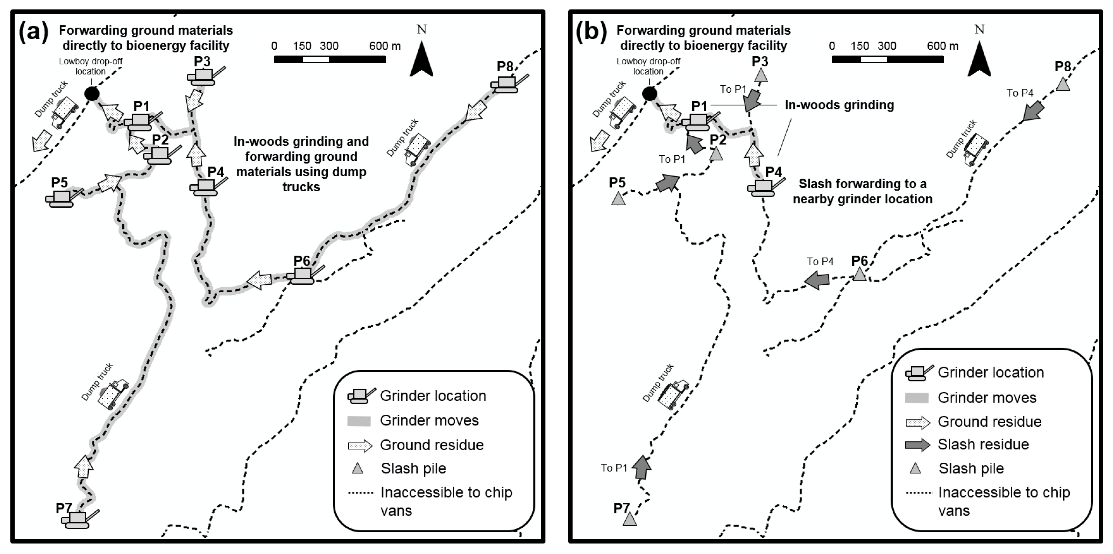
Conventional logistics were analyzed assuming that all the residues are processed by on-site grinding and the ground materials are transported to the bioenergy facility (Figure 6a). This system requires grinder mobilization to each residue pile and site construction for processing. In contrast, optimized logistics utilizes two grinder depots (P1 and P4) to process the residues from all other sites; instead of moving the grinder to each pile location, residues are forwarded to the selected grinder depots and processed at those sites (Figure 6b). This option results in less grinder mobilization and associated processing site construction.
Results from the cost analysis show that the processing and transportation costs are major components of both logistics configurations (Table 5). In conventional logistics, the machine mobilization and site construction costs are responsible for 23% of total cost due to frequent moves of the grinder and construction of processing sites, whereas in the optimized logistics they account for only 11% of total cost. However, slash forwarding to nearby grinder depots requires higher costs allocated to residue trucking and loading. This tradeoff resulted in total unit cost reduction from $39.6 bdt−1 to $37.0 bdt−1 for the given site conditions. The concentration yard is not used for processing and the transshipment option to chip vans is not selected. Grinding at the yard guarantees an increase in grinder productivity and a decrease in grinder mobilization cost, but those benefits must compensate for the additional costs incurred by concentration yard construction and low transportation efficiency to deliver bulky, unprocessed residues to the yard. Also, the reduction in transportation cost by transshipment must offset the additional handling costs, such as reloading of ground materials, front-end loader move-in cost and concentration yard construction cost.
A three dimensional relationship among residue pile volume, distance from pile to concentration yard, and unit cost for each pile indicates that the per unit extraction cost per pile is reduced if the amount of residue increases or the distance to the yard decreases (Figure 7). This tendency is observed in both conventional and optimized logistics, but the specific cost structure patterns between the two systems are quite different. The isocost contour lines of unit cost in the conventional logistics indicate that the unit cost is likely to decrease with volume (Figure 7a), while those lines in the optimized logistics indicate that the unit cost is more likely to increase with distance (Figure 7b). In general, economies of scale make grinding sensitive to residue volume; increasing the volume can help distribute the fixed costs of site construction and grinder mobilization over larger volumes of material. Slash forwarding is more sensitive to the transportation distance because the low bulk density of slash material reduces truck efficiency, thus increasing transportation cost. Given these characteristics, the unit cost of residue piles processed by on-site grinding in both logistics scenarios is largely affected by their volume rather than their distance, whereas the unit cost for residue piles forwarded to other grinding locations is affected primarily by distance. Also, note the difference in the rate of change for the two contour plots. Unit cost is more sensitive to the variables in the conventional logistics than in the optimized solution.
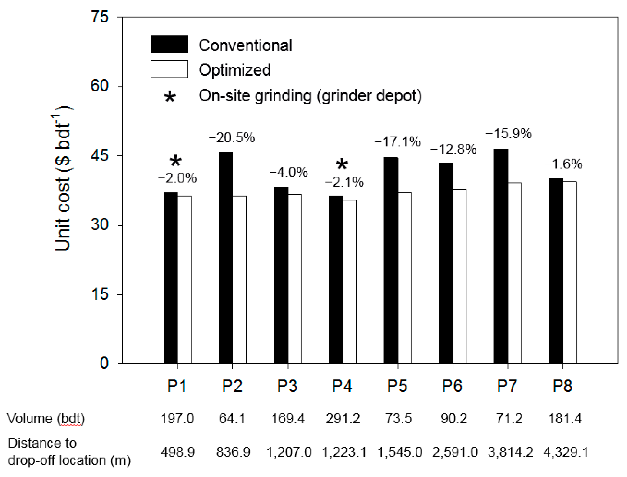
A high percentage of the reduction in unit cost is observed in residue piles selected to be forwarded to the grinder depots (Figure 8). These residue piles have relatively small volumes of material and, as a result, have comparatively higher fixed costs of grinder mobilization and site construction if they are processed at the pile locations. The selected grinder depots have relatively large amounts of volume and they are located shorter distances from the drop-off location. Their locations on the given road network and based on the given residue volume make them the best sites for processing, considering the tradeoffs among the cost components of processing, volume, and transportation. This small-scale problem consisted of 803 variables and 176 constraints, and it took only 0.1 s for the CPLEX to solve to optimality (Table 6).
5.2. Optimized Logistics with Different Volume Conditions
The optimal solution for biomass logistics of the study site varies with different volume conditions at pile locations, as well as feedstock demand at the bioenergy facility. If the residue volume is doubled at each pile location, the optimal solution indicates that an additional on-site grinding at P3 becomes the cost-efficient option. The new grinding location has enough volume to offset the fixed cost of site construction, and it is close enough to the other grinder depots (P1 and P4) to reduce grinder mobilization costs. A smaller amount of residue makes grinding location more sensitive to the site construction and movement of the grinder. When volume for each pile is set to half the original volume, the best option becomes forwarding all slash to one grinder depot (P1) for grinding, and then transporting ground material directly to the facility using small dump trucks. Transshipment to large chip vans does not occur in both volume cases mainly because of the high fixed cost of yard construction, which overwhelms the benefits from transshipment at the given volume and haul distance conditions.
When the total feedstock production is constrained to 700 bdt, the optimal logistics does not change in terms of on-site grinding locations (P1 and P4), but only two nearby slash piles (P2 and P3) are forwarded to P1 and there is no slash pile forwarded to P4. With these four piles, the volume constraint is met. On-site grinding at P4 is still required as it has enough volume and thus is more cost-efficient than slash forwarding to P1. When feedstock production is further constrained to 150 bdt, the best option becomes processing the extracted residues at one grinder location (P1) without any slash forwarding.
According to the costs analysis of different volume quantity scenarios, higher pile volumes or larger feedstock productions generally result in reduced unit cost (Table 7). The machine mobilization cost tends to be the greater proportion of total cost at the smaller amount of residue volume or feedstock production. Thus, careful design of logistics and machine selection is increasingly important when recovery operations are applied to low-volume conditions. This also has implications for harvest operations. When residues are burned for disposal, they are often piled in more widely dispersed, smaller piles, or even spread over the harvest areas (i.e., “lop and scatter”) to the extent possible or allowed by fuel treatment parameters. Clearly this practice is problematic if such residues are targeted for collection post hoc. The decision to use or dispose of residues should be made prior to the treatment so the residues can be handled appropriately to reduce costs based on the anticipated logistics. This is an obvious point from a harvest planning perspective, but one that is often ignored in practice, especially in locations with weak or ephemeral biomass markets.
Our results also imply that slash-forwarding could be a good option for tree-length, ground-based harvesting systems because they tend to generate many relatively small residue piles. In contrast, in-woods grinding could be a more efficient option when whole-tree, cable logging systems are applied that typically leave large slash piles at relatively large size landings. Moisture content of residues would also likely affect the optimal feedstock logistics because of the interaction between volume and weight. Small dump trucks are typically constrained by volume rather than weight [11], and a decrease in moisture content would make forwarding ground residues more favorable than unprocessed residues because trucks can realize a higher payload in the same cycle by carrying higher bulk density materials. This tradeoff also applies to different truck types and capacities. Recall that the trucks used in this case study were based on those used in [11]. Different trucks, such as high-capacity off-road dump trucks, are available, and may result in similarly different outcomes if bulky, dry materials are more efficiently transported as ground residues.
5.3. Model Application for a Larger Project Area
We applied the optimization model to 58 slash pile locations with a total volume of 7691 bdt dispersed across a larger project area to further demonstrate and evaluate model performance (Figure 9). A hypothetical concentration yard was pre-selected based on terrain and site conditions. The optimal solution indicates that all residue piles located in the southeast of the project area (3800 bdt) should be forwarded to the concentration yard where they can be ground directly into large chip vans. For the remainder of the residues, located in the northwest of the area, the residue piles are forwarded to two grinder depots selected for on-site grinding. The ground residues are then transported to the concentration yard using dump trucks due to the inaccessibility of the sites to large chip vans, and then transshipped to large chip vans at the concentration yard for long-haul transportation to the bioenergy facility (36 km). It is noteworthy that the optimized logistics selects to transship the ground residues to chip vans to improve transportation efficiency to the bioenergy facility. In this example, the economic benefit of transshipment is large enough to offset additional handling costs of reloading at the yard. This seems to go against the conventional wisdom that double handling material is almost always more costly compared to configurations that involve fewer unloading and reloading cycles. If compared with the conventional logistics (i.e., on-site grinding at each residue pile location), our cost estimates show that the optimized system is able to reduce the total logistics costs by 11%, from $44.7 bdt−1 to $39.9 bdt−1.
An increase in problem size results in a linear increase in the number of constraints but an exponential increase in the number of variables in the MIP model (Table 6). This large problem example with 58 pile locations took 6.6 s for the CPLEX to solve to optimality.
6. Conclusions
We applied a mixed-integer programming approach coupled with a network algorithm to a biomass feedstock logistics problem where the most cost-efficient grinder locations and processing and transportation operations were unknown. According to the results of our model applications, the slash forwarding option is generally beneficial if a residue pile is relatively small (e.g., residue piles P2, P5, P6 and P7 in Table 2) or located close to a processing site (e.g., P2, P3, P5, and P6 in Figure 6b), while in-woods grinding is more cost-efficient in situations where residue volume is relatively large and where forwarding residues from nearby sites can guarantee the economic benefits of grinding at the grinder depot (e.g., P1 and P4). The transshipment option is appropriate if the increase in transportation efficiency compensates the additional handling costs caused by reloading ground material and by front-end loader mobilization, as well as yard construction if the yard is used only for the transshipment.
Conventionally, forest contractors have used in-woods grinding in residue recovery operations, but our results showed that using this mixed-integer approach in decision making can reduce the cost of the operation with some unconventional modifications. In the first model application with a small project area, the optimized logistics forwards residues to the selected grinder depots instead of moving the grinder to each pile location, and this change results in a 7% unit cost reduction compared to the conventional logistics. For the larger project area covered in the second model application, optimized logistics reduces the unit cost by 11% compared to the conventional system. These reductions are important to forest contractors because forest residues are underutilized due to high processing, handling and transportation costs relative to their value. A decision that optimizes logistics to improve the efficiency of operations can make forest biomass utilization more economically viable, meaning more biomass can be sold profitably and less burned for disposal.
Another important consideration when contractors are faced with these options is the situation where multiple businesses are involved in the recovery operation. It is possible that a contractor who owns and operates a grinder subcontracts transportation duties to an independent trucking company. This may introduce conflicts regarding the unit of payment provided to the trucking company. Depending on the contract provisions, the conventional system can be advantageous for the trucking company because transportation efficiency will be higher than forwarding slash. Conversely, grinding at a few of candidate sites is advantageous for the owner of the grinder because grinder mobilization costs can be avoided. Our model can resolve this conflict by providing a solution to the problem that represents the least expensive alternative on a common unit of cost for the entire system.
The MIP approach introduced in this study is unique in three ways. It formulates the pile-to-pile grinder movement using binary variables to account for equipment mobilization costs. To reduce the problem size, our model combines the shortest path algorithm with MIP, and formulates the problem based on the least-cost routes predetermined between possible pairs of nodes. Lastly, our model is one of few efforts to expand the application boundary of optimization to assist in forest operational decisions where high precision data and models are usually required to represent problem details. With advanced sensors and information technology used in forest operations, the data are growing both in quantity and quality, and the development of optimization applications for forest operations is expected to grow. This study provides an example of integrating detailed field data with mathematical optimization for specific operational decisions.
The application of our problem formulation for equipment mobilization is limited to hierarchical, tree-shaped road networks. Although this is common in many real-world forestry settings where most adjacent log landings share main haul direction or are accessed through a spur road, such as in hilly and mountainous terrain, our formulation would not be suitable for road systems that do not conform to this general layout, such as a grid network.
Our future research efforts include incorporating this optimization model into a practical decision support system that can be used easily and broadly by land managers and the industry. Combined with geographic information systems and a data entry user-interface, this optimization model will provide a complete tool that can help land managers and forest contractors analyze different feedstock logistics options and identify the most cost-efficient practices given conditions and objectives. Such improvements would contribute significantly to efficient expansion of the bioeconomy using forest biomass feedstocks.
Acknowledgments
This research was supported by the Agriculture and Food Research Initiative Competitive Grant No. 2013-68005-21298 from the USDA National Institute of Food and Agriculture through the Bioenergy Alliance Network of the Rockies (BANR), and a USDA Forest Service Rocky Mountain Research Station Grant No. 16-JV-11221636-106. The authors thank John Twitchell and Russ Gross at Colorado State Forest Service for providing their insights and data for this study.
Author Contributions
Woodam Chung, Hee Han and Nathaniel Anderson conceived and designed the model; Hee Han, Woodam Chung and Lucas Wells developed the model; Hee Han and Lucas Wells performed the analysis; Hee Han, Woodam Chung and Lucas Wells wrote the paper; Woodam Chung and Nathaniel Anderson provided analytical expertise and editorial contributions.
Conflicts of Interest
The authors declare no conflict of interest.
References
- US Department of Energy. 2016 Billion-Ton Report: Advancing Domestic Resources for a Thriving Bioeconomy, Volume 1: Economic Availability of Feedstocks; US Department of Energy: Washington, DC, USA, 2016.
- Verkerk, P.J.; Anttila, P.; Eggers, J.; Lindner, M.; Asikainen, A. The realisable potential supply of woody biomass from forests in the European Union. For. Ecol. Manag. 2011, 261, 2007–2015. [Google Scholar] [CrossRef]
- Welfle, A. Balancing growing global bioenergy resource demands—Brazil’s biomass potential and the availability of resource for trade. Biomass Bioenergy 2017, 105, 83–95. [Google Scholar] [CrossRef]
- Anderson, N.; Mitchell, D. Forest operations and woody biomass logistics to improve efficiency, value, and sustainability. Bioenergy Res. 2016, 9, 518–533. [Google Scholar] [CrossRef]
- Harrill, H.; Han, H.-S. Application of hook-lift trucks in centralized logging slash grinding operations. Biofuels 2010, 1, 399–408. [Google Scholar] [CrossRef]
- Zamora-Cristales, R.; Sessions, J.; Murphy, G.; Boston, K. Economic impact of truck–machine interference in forest biomass recovery operations on steep terrain. For. Prod. J. 2013, 63, 162–173. [Google Scholar] [CrossRef]
- Marchi, E.; Magagnotti, N.; Berretti, L.; Neri, F.; Spinelli, R. Comparing terrain and roadside chipping in Mediterranean pine salvage cuts. Croat. J. For. Eng. 2011, 32, 587–598. [Google Scholar]
- Lauer, C.; McCaulou, J.C.; Sessions, J.; Capalbo, S.M. Biomass supply curves for western juniper in Central Oregon, USA, under alternative business models and policy assumptions. For. Policy Econ. 2015, 59, 75–82. [Google Scholar] [CrossRef]
- Yemshanov, D.; McKenney, D.W.; Fraleigh, S.; McConkey, B.; Huffman, T.; Smith, S. Cost estimate of post harvest forest biomass supply for Canada. Biomass Bioenergy 2014, 69, 80–94. [Google Scholar] [CrossRef]
- Zamora-Cristales, R.; Sessions, J.; Boston, K.; Murphy, G. Economic optimization of forest biomass processing and transport in the Pacific Northwest USA. For. Sci. 2015, 61, 220–234. [Google Scholar] [CrossRef]
- Anderson, N.; Chung, W.; Loeffler, D.; Jones, J.G. A productivity and cost comparison of two systems for producing biomass fuel from roadside forest treatment residues. For. Prod. J. 2012, 62, 222–223. [Google Scholar] [CrossRef]
- Shabani, N.; Akhtari, S.; Sowlati, T. Value chain optimization of forest biomass for bioenergy production: A review. Renew. Sust. Energ. Rev. 2013, 23, 299–311. [Google Scholar] [CrossRef]
- Johnson, D.M.; Jenkins, T.L.; Zhang, R. Methods for optimally locating a forest biomass-to-biofuel facility. Biofuels 2012, 3, 489–503. [Google Scholar] [CrossRef]
- Nagel, J. Determination of an economic energy supply structure based on biomass using a mixed-integer linear optimization model. Ecol. Eng. 2000, 16, 91–102. [Google Scholar] [CrossRef]
- Shabani, N.; Sowlati, T. A mixed integer non-linear programming model for tactical value chain optimization of a wood biomass power plant. Appl. Energ. 2013, 104, 353–361. [Google Scholar] [CrossRef]
- Shabani, N.; Sowlati, T.; Ouhimmou, M.; Rönnqvist, M. Tactical supply chain planning for a forest biomass power plant under supply uncertainty. Energy 2014, 78, 346–355. [Google Scholar] [CrossRef]
- Flisberg, P.; Frisk, M.; Rönnqvist, M. FuelOpt: A decision support system for forest fuel logistics. J. Oper. Res. Soc. 2012, 63, 1600–1612. [Google Scholar] [CrossRef]
- Han, S.-K.; Murphy, G.E. Solving a woody biomass truck scheduling problem for a transport company in Western Oregon, USA. Biomass Bioenergy 2012, 44, 47–55. [Google Scholar] [CrossRef]
- Dijkstra, E.W. A note on two problems in connexion with graphs. Numer. Math. 1959, 1, 269–271. [Google Scholar] [CrossRef]
- IBM ILOG. CPLEX® 12.6; IBM Corp: New York, NY, USA, 2015. [Google Scholar]
- Wells, L.A.; Chung, W.; Anderson, N.M.; Hogland, J.S. Spatial and temporal quantification of forest residue volumes and delivered costs. Can. J. For. Res. 2016, 46, 832–843. [Google Scholar] [CrossRef]
- Loeffler, D.; Anderson, N. Emissions tradeoffs associated with cofiring forest biomass with coal: A case study in Colorado, USA. Appl. Energy 2014, 113, 67–77. [Google Scholar] [CrossRef]
- Twitchell, J.; Colorado State Forest Service, Walden, CO, USA. Personal communication, 2017.
- Fight, R.D.; Zhang, X.; Hartsough, B.R. Users Guide for STHARVEST: Software to Estimate the Cost of Harvesting Small Timber; USDA Forest Service General Technical Reports; US Department of Agriculture: Washington, DC, USA, 2003.
- Colorado Department of Labor and Employment. Occupational Employment Statistics Employment and Wage Estimates; Colorado Department of Labor and Employment: Denver, CO, USA, 2016. Available online: www.colmigateway.com (accessed on 9 November 2016).
- Bruce, J.; Han, H.-S.; Akay, A.E.; Chung, W. ACCE: Spreadsheet-based cost estimation for forest road construction. West. J. Appl. For. 2011, 26, 189–197. [Google Scholar]
- Zamora-Cristales, R. Economic Optimization of Forest Biomass Processing and Transport. Ph.D. Thesis, Oregon State University, Corvallis, OR, USA, 2013. [Google Scholar]
- Systat Software. SigmaPlot 13.0; Systat Software: San Jose, CA, USA, 2016. [Google Scholar]
Figure 1.
In-woods grinding (a), slash forwarding (b), and a combination system of both options (c). All three options assume forest residue piles are inaccessible to large chip vans due to poor road conditions. Small dump trucks must be used to forward ground materials or slash residues at least to where large chip vans can access (i.e., concentration yard). Note that it is also an option to directly transport ground materials to bioenergy facility using dump trucks.
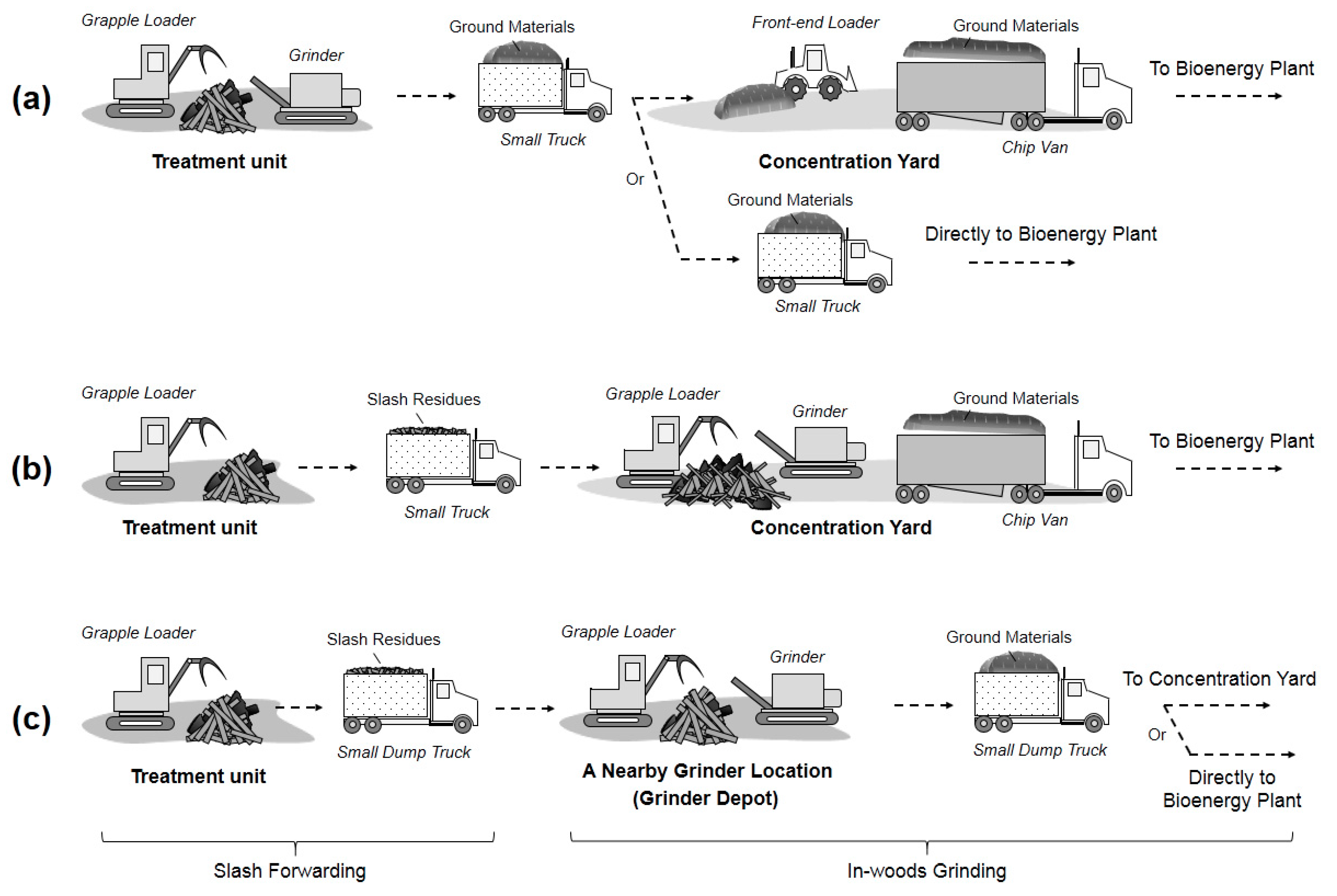
Figure 2.
A flow chart diagram presenting three model components, required data and solution procedures used in the optimization model.
Figure 2.
A flow chart diagram presenting three model components, required data and solution procedures used in the optimization model.
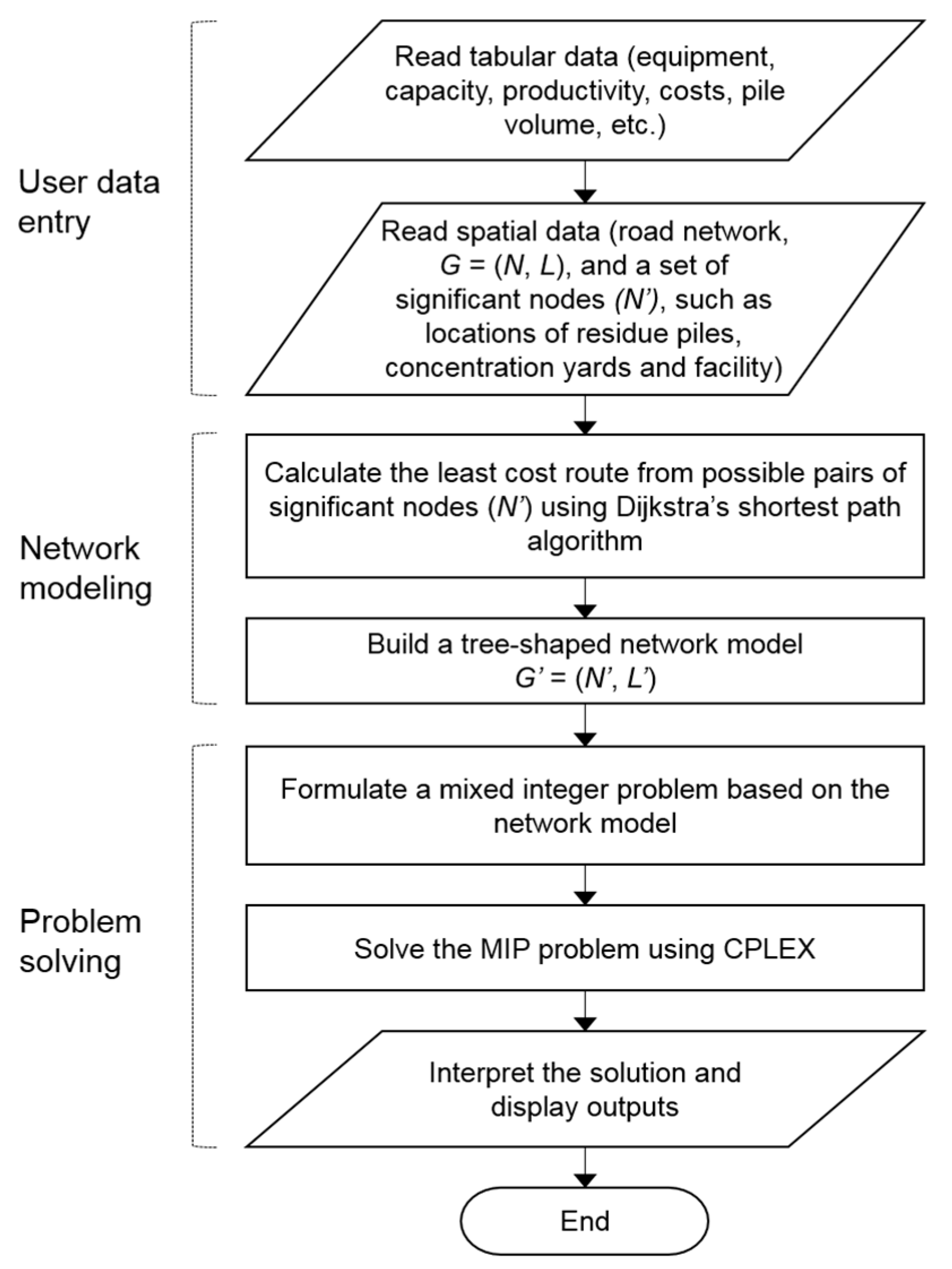
Figure 3.
A network diagram representing a hypothetical configuration of in-woods grinding, slash forwarding, and large chip van transportation options.
Figure 3.
A network diagram representing a hypothetical configuration of in-woods grinding, slash forwarding, and large chip van transportation options.

Figure 4.
An example illustrating machine (e.g., grinder) mobilization for a hierarchical, tree-shaped road network. The numbered arrows indicate the move sequence and direction of the grinder as it visits each pile location for processing.
Figure 4.
An example illustrating machine (e.g., grinder) mobilization for a hierarchical, tree-shaped road network. The numbered arrows indicate the move sequence and direction of the grinder as it visits each pile location for processing.

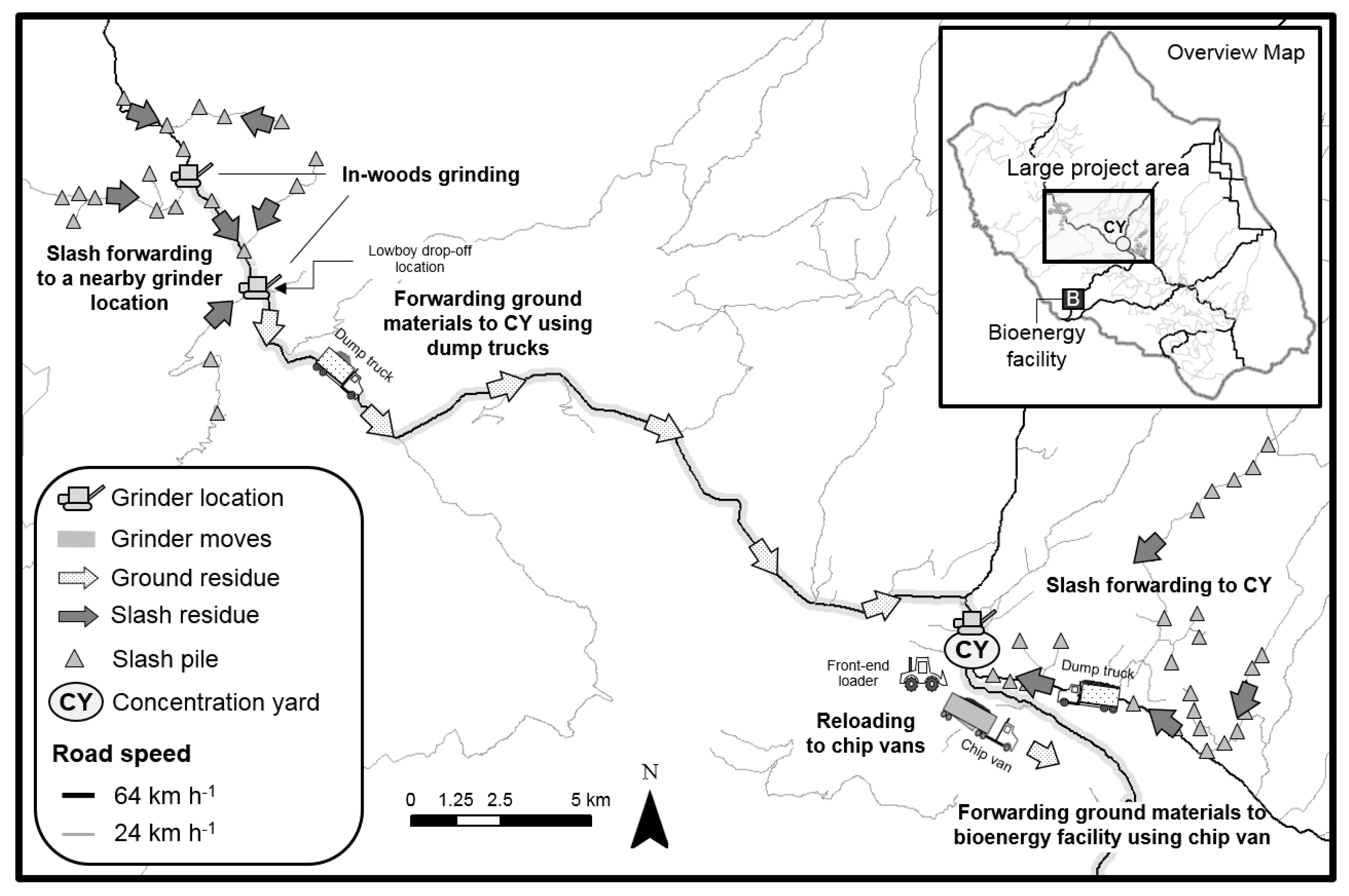
Figure 5.
Spatial locations of forest residue piles, lowboy drop-off, and potential concentration yard location for a small area of Uncompahgre National Forest (UNF), Colorado. A bioenergy facility is assumed to be located approximately 36 km southwest from the concentration yard at a coal-fired power plant.

Figure 6.
Conventional (a) and optimized (b) feedstock logistics presenting biomass flow and selected on-site grinding locations.
Figure 6.
Conventional (a) and optimized (b) feedstock logistics presenting biomass flow and selected on-site grinding locations.

Figure 7.
Isocost contour plots of conventional (a) and optimized (b) logistics costs. These plots present a 3-dimensional relationship with residue volume (x-axis), distance to concentration yard (y-axis), and unit cost (grayscale with marked contours). Black dots (P1 through P8) represent pile locations in terms of residue volume and distance to concentration yard. The darker regions indicate higher unit cost and number in the white box shows the unit cost at each contour.
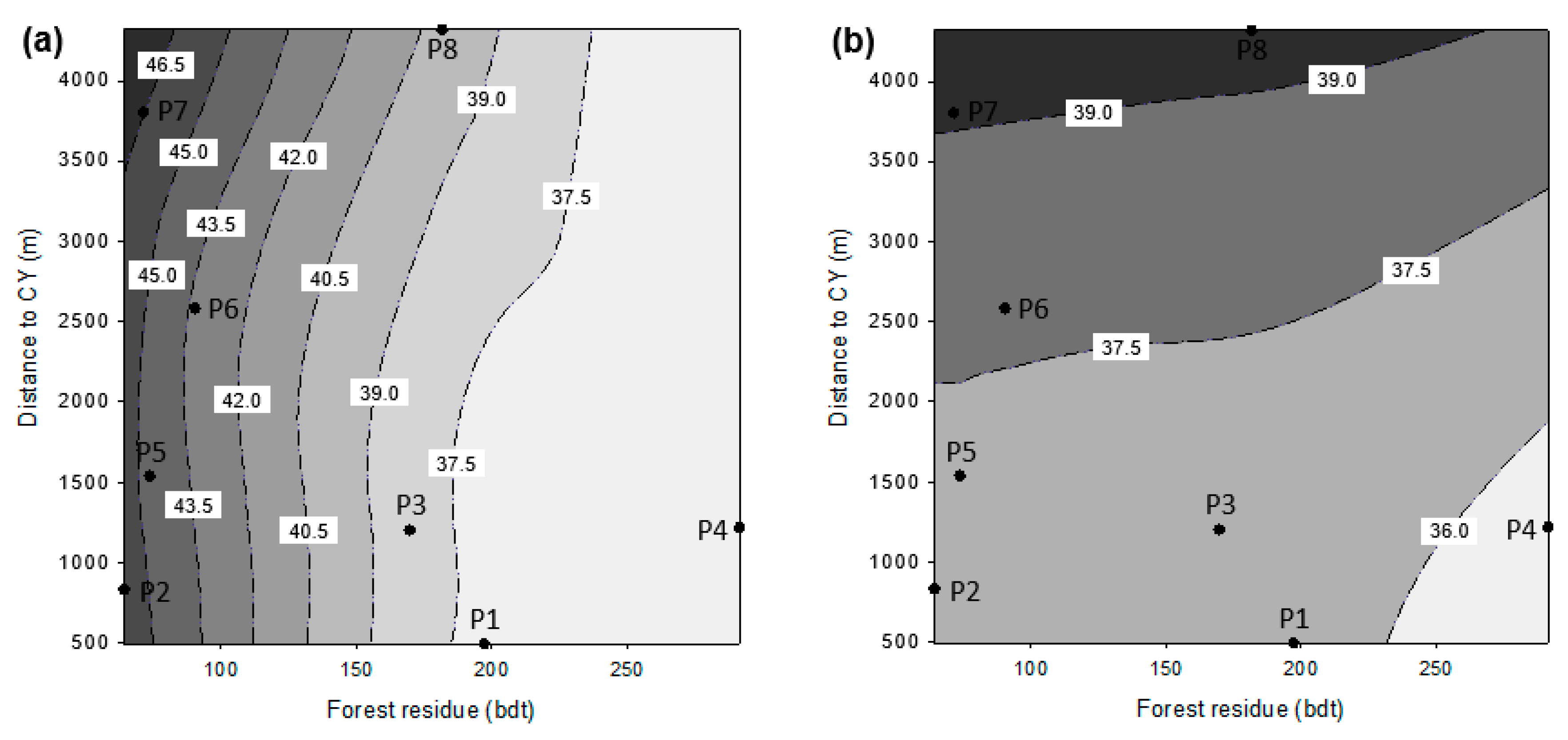
Figure 8.
Unit costs of conventional and optimized logistics at each residue pile. The number above the bars indicates the percentage reduction in unit cost per pile attributable to optimized logistics.
Figure 8.
Unit costs of conventional and optimized logistics at each residue pile. The number above the bars indicates the percentage reduction in unit cost per pile attributable to optimized logistics.

Figure 9.
Optimized feedstock logistics for a larger project area (58 log landings) presenting biomass flow, selected on-site grinding locations, and the use of concentration yard for transshipment.
Figure 9.
Optimized feedstock logistics for a larger project area (58 log landings) presenting biomass flow, selected on-site grinding locations, and the use of concentration yard for transshipment.


Table 1.
Sets, decision variables, and parameters of the optimization model.
| Element | Description |
|---|---|
| Sets | |
| Set of residue pile locations | |
| Set of concentration yards | |
| Set of bioenergy facilities | |
| Set of intermediate nodes that are not a residue pile, a concentration yard, or a bioenergy facility | |
| Set of nodes (i.e., ) | |
| Set of directed links connecting the nodes in | |
| Set of machines required for handling slash residue (i.e., grapple loader) | |
| Set of machines required for producing ground residue (i.e., grinder and grapple loader) | |
| Set of machines required for handling ground residue (i.e., front-end loader) | |
| Set of equipment (i.e., ) | |
| Set of directed links included in the shortest route from u to v | |
| Decision variables | |
| Flow of slash residue transported over the shortest route from i to j (bdt) | |
| Flow of ground residue transported over the shortest route from i to j (bdt) | |
| Flow of slash residue ground at concentration yard j and transported to bioenergy facility k (bdt) | |
| Flow of ground residue transshipped at concentration yard j and transported to bioenergy facility k (bdt) | |
| 0, 1 integer variable over directed link ab used for mobilization of machine m | |
| 0, 1 integer variable if a machine m is located at node u | |
| Parameters | |
| Grinding cost at location i ($ bdt−1) | |
| Transportation cost of slash residue on route ij ($ bdt−1) | |
| Slash residue loading cost at location i ($ bdt−1) | |
| Transportation cost of ground residue on route ij ($ bdt−1) | |
| Ground residue loading cost at location i ($ bdt−1) | |
| Move-in costs of machine m over directed link ab ($) | |
| Site construction cost if a machine m is located at node u for processing ($) | |
| Pile volume at source node i (bdt) | |
| Number of directed links included in the shortest path from u to v | |
| Minimum required volume (ground residue) to be delivered to bioenergy facility j (bdt) |
Table 2.
Residue volumes in bone dry tons (bdt) at each pile location and distances to lowboy drop-off location.
Table 2.
Residue volumes in bone dry tons (bdt) at each pile location and distances to lowboy drop-off location.
| Residue Pile | Volume (bdt) | Distance to Lowboy Drop-Off Location (m) |
|---|---|---|
| P1 | 197.0 | 499 |
| P2 | 64.1 | 837 |
| P3 | 169.4 | 1207 |
| P4 | 291.2 | 1223 |
| P5 | 73.5 | 1545 |
| P6 | 90.2 | 2591 |
| P7 | 71.2 | 3814 |
| P8 | 181.4 | 4329 |
| Total | 1138.0 | - |
Table 3.
Hourly cost and productivity of equipment and truck capacities used in the model applications.
Table 3.
Hourly cost and productivity of equipment and truck capacities used in the model applications.
| Cost | Equipment | ||||
|---|---|---|---|---|---|
| Grinder | Grapple Loader | Front-End Loader | Dump Truck | Chip Van | |
| Ownership cost ($ SMH−1) | 72.32 | 28.30 | 18.19 | 7.55 | 10.48 |
| Operating cost ($ SMH−1) | 247.24 | 61.40 | 62.32 | 44.37 | 81.85 |
| Labor | 28.18 | 28.18 | 28.18 | 28.18 | 28.18 |
| Fuel and lubricants | 82.30 | 18.22 | 24.49 | 12.82 | 48.98 |
| Repair and maintenance | 47.06 | 15.00 | 9.65 | 3.37 | 4.69 |
| Loader to feed grinder | 89.70 | - | - | - | - |
| Total cost ($ SMH−1) | 319.56 | 89.70 | 80.51 | 51.92 | 92.33 |
| Productivity 1 (bdt SMH−1) | 31.50 2 26.71 3 | 45.72 | 62.85 | - | - |
| Truck capacity 1 (bdt) | - | - | - | 4.60 4 6.21 5 | 23.40 5 |
1 Adapted and updated from Anderson et al. [11]; 2 Grinding at concentration yard; 3 On-site grinding; 4 Slash residue; 5 Ground residue.
Table 4.
Travel speeds of equipment applied in the model.
| Travel Type | Equipment Speed (km∙h−1) | |||
|---|---|---|---|---|
| Lowboy | Grapple Loader | Grinder | Front-End Loader 1 | |
| Loaded travel | 40.2 | - | - | - |
| Empty travel | 64.4 | - | - | - |
| Walk | - | 5.5 | 2.4 | - |
1 Front-end loader is transported to the concentration yard using a lowboy trailer and then stays at the yard.
Table 5.
Results of a cost analysis for conventional and optimized logistics.
| Logistics | Conventional (A) | Optimized (B) | Difference (B−A) | |||
|---|---|---|---|---|---|---|
| No. of on-site grinding locations used | 8 | 2 | −6 | |||
| Cost | ($) | (%) | ($) | (%) | ($) | (%) |
| Processing | 13,610.5 | 30.2 | 13,610.5 | 32.3 | 0.0 | 0.0 |
| Transportation | 21,302.6 | 47.3 | 22,753.1 | 54.1 | 1450.5 | 6.8 |
| Loading, pile | 0.0 | 0.0 | 1273.6 | 3.0 | 1273.6 | - |
| Loading, concentration yard | 0.0 | 0.0 | 0.0 | 0.0 | 0.0 | 0.0 |
| Machine mobilization | 3736.6 | 8.3 | 2875.5 | 6.8 | −861.1 | −23.0 |
| Site construction | 6400.0 | 14.2 | 1600.0 | 3.8 | −4800.0 | −75.0 |
| Total | 45,049.7 | 100.0 | 42,112.7 | 100.0 | −2937.0 | −6.5 |
| Unit cost ($ bdt−1) | 39.6 | 37.0 | −2.6 | −6.6 | ||
Table 6.
Problem size and solution time of the two model applications presented in this study.
| Problem | Small-size Problem | Large-size Problem |
|---|---|---|
| Nodes | ||
| Log landings | 8 | 58 |
| Intermediate nodes 1 | 16 | 163 |
| Concentration yard | 1 | 1 |
| Bioenergy facility | 1 | 1 |
| Total | 26 | 223 |
| Variables | ||
| Continuous 2 | 702 | 49,952 |
| Binary | 101 | 889 |
| Total | 803 | 50,841 |
| Constraints | 176 | 1555 |
| Solution time (s) | 0.1 | 6.6 |
1 Road junctions or locations where engineered road speed changes; 2 also represents the total number of links.
Table 7.
Results of a cost analysis for different volume quantity scenarios.
| Volume Scenario | Pile Volume | Feedstock Production Constraint | ||||||||
|---|---|---|---|---|---|---|---|---|---|---|
| Current | Double | Half | ||||||||
| Volume required to be processed | 1138.0 | 2276.0 | 569.0 | 700.0 | 150.0 | |||||
| No. of on-site grinding locations selected | 2 | 3 | 1 | 2 | 1 | |||||
| ($) | (%) | ($) | (%) | ($) | (%) | ($) | (%) | ($) | (%) | |
| Cost | ||||||||||
| Processing | 13,610.5 | 32.3 | 27,221.0 | 34.3 | 6805.2 | 29.7 | 8372.0 | 32.0 | 1794.0 | 25.9 |
| Transportation | 22,753.1 | 54.1 | 44,836.1 | 56.6 | 11,688.4 | 51.1 | 13,089.8 | 50.1 | 2666.7 | 38.5 |
| Loading at pile | 1273.6 | 3.0 | 1883.2 | 2.4 | 922.1 | 4.0 | 415.1 | 1.6 | 0.0 | 0.0 |
| Loading at yard | 0.0 | 0.0 | 0.0 | 0.0 | 0.0 | 0.0 | 0.0 | 0.0 | 0.0 | 0.0 |
| Mobilization | 2875.5 | 6.8 | 2946.3 | 3.7 | 2685.6 | 11.7 | 2653.3 | 10.2 | 1665.9 | 24.1 |
| Construction | 1600.0 | 3.8 | 2400.0 | 3.0 | 800.0 | 3.5 | 1600.0 | 6.1 | 800.0 | 11.5 |
| Total | 42,112.7 | 100.0 | 79,286.6 | 100.0 | 22,901.3 | 100.0 | 26,130.2 | 100.0 | 6926.6 | 100.0 |
| Unit cost ($ bdt−1) | 37.0 | 34.8 | 40.3 | 37.3 | 46.2 | |||||
© 2018 by the authors. Licensee MDPI, Basel, Switzerland. This article is an open access article distributed under the terms and conditions of the Creative Commons Attribution (CC BY) license (http://creativecommons.org/licenses/by/4.0/).
Share and Cite
MDPI and ACS Style
Han, H.; Chung, W.; Wells, L.; Anderson, N. Optimizing Biomass Feedstock Logistics for Forest Residue Processing and Transportation on a Tree-Shaped Road Network. Forests 2018, 9, 121. https://doi.org/10.3390/f9030121
AMA Style
Han H, Chung W, Wells L, Anderson N. Optimizing Biomass Feedstock Logistics for Forest Residue Processing and Transportation on a Tree-Shaped Road Network. Forests. 2018; 9(3):121. https://doi.org/10.3390/f9030121
Chicago/Turabian StyleHan, Hee, Woodam Chung, Lucas Wells, and Nathaniel Anderson. 2018. "Optimizing Biomass Feedstock Logistics for Forest Residue Processing and Transportation on a Tree-Shaped Road Network" Forests 9, no. 3: 121. https://doi.org/10.3390/f9030121
Note that from the first issue of 2016, this journal uses article numbers instead of page numbers. See further details here.