Leaf Trait Variation with Environmental Factors at Different Spatial Scales: A Multilevel Analysis Across a Forest-Steppe Transition


Institute of Soil and Water Conservation, Northwest A & F University, 26 Xinong Road, Yangling 712100, Shaanxi, China
*
Author to whom correspondence should be addressed.
Forests 2018, 9(3), 122; https://doi.org/10.3390/f9030122
Submission received: 31 December 2017
/
Revised: 15 February 2018
/
Accepted: 3 March 2018
/
Published: 6 March 2018
(This article belongs to the Special Issue Forest Policy and Biodiversity Strategy: The Relevance of Forest Genetic Resources)
Abstract
:In mountain areas, the distribution of plant communities is affected by both regional and microhabitat conditions. The degree to which these different spatial factors contribute to plant communities is not well understood, because few studies have used a uniform sampling methodology to measure trait variation across the range of ecological scales. In this study, a stratified sampling method was used to study community weighted leaf traits and environment factors at different spatial (transect and plot) scales. We measured 6 leaf traits (specific leaf area, leaf tissue density, leaf thickness, leaf carbon, nitrogen and phosphorus content) in 258 communities from 57 sites in 9 transects nested within 3 vegetation zones. These communities are located in the loess hilly and gully area of the Yanhe river watershed. We coupled climatic factors at the transect scale with topographic and edaphic factors at the plot scale using multilevel regression modeling to analyze the trait variation associated with spatial scales. At the transect scale, the mean annual rainfall showed a highly significant positive effect on the leaf nitrogen concentration (LNC) (p < 0.01), while it had a highly significant negative effect on leaf thickness (LT) and leaf tissue density (LTD) (p < 0.001) and a significant negative effect on leaf carbon concentration (LCC) (p < 0.05), explaining 10.91%, 36.08%, 57.25% and 66.01% of LTD, LT, LCC and LNC variation at transect scale respectively. At a plot scale, the slope aspect showed a highly significant positive effect on specific leaf area (SLA) and LNC but a highly significant negative effect on LT and LTD. The soil water content had a significant negative effect on LT (p < 0.05) and LTD (p < 0.001) while soil organic matter showed a positive effect on SLA (p < 0.001) and LNC (p < 0.01). Totally, plot scale variables explained 7.28%, 43.60%, 46.43%, 75.39% and 81.17% of LCC, LT, LNC, LTD and SLA variation. The elevation showed positive effect only on LCC (p < 0.05). The results confirmed the existence of consistent trait–environment relationships at both transect and plot scales. These trait–environment relationships at different spatial scales will provide mechanistic understanding on the vegetation community assembly in the study area. Practically, ignoring trait variation within transects will underestimate roles of microhabitat filters in community assembly, and leads to the homogenization of restoration species. This will be like the past restoration plans and programs, causing serious environmental problems such as dwarf trees and soil desiccation.
1. Introduction
Environmental filtering, one of the key community assembling processes, constrains species establishment through selection on functional traits [1,2]. During this process, habitats act as filters removing species lacking trait attributes for persisting under a given environment [3]. As a result, co-occurring species in a given habitat are assumed to exhibit similar ecological strategies and share similar traits [1,3,4], i.e., that environment filtering leads to the trait convergence of co-occurring species and thus shapes the community structure in a particular habitat [5,6]. Investigating trait–environment linkages or consistent associations between sets of plant attributes and certain environmental conditions would provide insights into the mechanisms of species coexistence and species distribution [3].
Spatially, multiple environmental filters exist and they may operate at a hierarchy of scales [5]. At the regional and global scales, many studies have demonstrated strong correlations between leaf-level traits and climate gradients across large spatial scales [7,8,9,10,11]. However, these correlations may not be consistent at smaller scales. Some studies indicated that the relationship between leaf-level traits and climate gradients may be weaker [12] or non-existent [13] at smaller scales while some studies indicate that the processes at smaller scales may be of equal or greater importance in determining the trait variation [1,14]. These uncertainties in correlations between leaf traits and environment conditions may underestimate the roles of small scale filters in community assembly [14], thus preventing the investment of restoration and management efforts in right scales.
In mountainous areas, the situation can be more complicated. Topographic heterogeneity creates a wide variety of habitats, and is one of the most important determinants of plant species diversity in these areas [15,16,17,18]. Even within short distances, the topographically complex terrain can create a mosaic of diverse microclimates, and exert strong effects on plant species diversity and trait variation [19]. A study by Bergholz showed that environmental heterogeneity at a relatively fine scale (1 m2) still has important filtering effect on traits (trait convergence) and influence the species assembly [20]. However, the environmental filters at different spatial scales don’t affect the assembling process independently but act in a hierarchy way [3,21]. Regional climate may act as a first level filters and the topography induced microhabitat act as the second level filters [3]. For example, in the loess hilly and gully area of China, the vegetation distribution is mainly controlled by regional climate pattern. Zou classified the vegetation in this region into forest zone, forest-steppe zone and steppe zone according to rainfall and temperatures changes [22]. However, topographic changes in this region also result in a wide variety of habitats, which enable the persistence of some tree and shrub species in gullies and lower slopes in steppe and forest-steppe zones while some herb communities may develop in mountain tops in forest zone. So the vegetation pattern in this area is characterized by a mosaic of zonal vegetation (filtered by regional climate) and azonal vegetation (filtered by microhabitat) [23,24]. Unfortunately, the filtering effect of local microhabitat filters on the community assembly is not well understood because few studies explore the existence of consistence of trait–environmental relationships at micro scale in this region. Most of the restoration plans and management decisions are still based on the vegetation zoning map [25], although it has led to serious environmental problems such as dwarf trees and soil desiccation [25,26].
Solving this problem is challenging since few studies have used a uniform sampling methodology to measure trait variation across the range of ecological scales [14]. Moreover, when scaling up, the hierarchy structure of the ecological data make it difficult to use the traditional multiple linear model to describe the relationship between traits and environmental factors across ecological scales [27]. In these situations, the spatial autocorrelation and hierarchy of ecological data are usually overlooked. This has contributed to additional uncertainty in determining linkages between plant traits and environment conditions [28,29]. Fortunately, the recent use of multilevel models in ecology provides a solution to this problem. These models give adequate consideration to the spatial autocorrelation and hierarchy of ecological data, have a more subtle decomposition for the error term to separate the variation between groups and within groups, and help explain the relative variation at various levels of the observed values [30].
So, to quantify the contributions of environmental factors at different scales to trait variation and incorporate constrains of local environmental filters into restoration planning, we selected natural plant communities in the loess hilly-gully region of the Yanhe River basin, and used a multilevel/hierarchical model to study the relationship between plant traits and environmental filters at different scales. We selected leaf traits for our study, because leaf traits are closely related to the capture and use of resources [31,32], aboveground biomass production [33], survival strategies [34] and adaptability of plant species [35], are primarily important for ecological processes, and mostly used functional traits in ecological studies. Our objectives are (1) to quantitatively determine trait–environment relationships at different spatial scales in the Yanhe River catchment; and (2) to find if there exist consistent trait–environment relationships at micro scale, thus helping understand the environmental filters at different spatial scales in community assembly in the loess and gully area.
2. Materials and Methods
2.1. Study Area
The study area is located in Yanhe River in the northern Shaanxi province of China. The Yanhe River is a primary tributary of the Yellow River. The Yanhe River basin area is a typical hilly-gully loess region [36]. The total length of Yanhe River is 286.9 km with an area of 7687 km2. The average elevation is 1371.9 m, and the average slope is 4.3‰. The drainage density is about 4.7 km/km2. The dominant soil type is loess loamy soil with loose texture and prone to erosion. The climate is continental semi-arid monsoon with an annual mean temperature of 8.8 °C and annual average rainfall of 505 mm, 70% of which falls between May and September. Within the catchment, temperature and rainfall are not uniform. From southeast to northwest, rainfall and temperature gradually decreases. With rainfall and temperature changes, vegetation changes regionally with a forest zone in the southeast, a forest-steppe transition zone in the middle, and a typical steppe zone in the northwest (Figure 1). However, due to the topographic changes, the vegetation pattern in the watershed is characterized by a mosaic of zonal vegetation (filtered by regional climate) and azonal vegetation (filtered by microhabitat) [23,24], with azonal vegetation patches nested in zonal vegetation.
2.2. Sampling Design and Community Investigation
According to the nested structure of the sample sites and multilevel modeling theory, we collected data on plant functional traits and environmental factors from July to August 2014 using a stratified sampling design. We first stratified the entire catchment into three zones based on the study by Zou [22]. Within each zone, three transects were established to cover different slope aspects and positions (Figure 1). Along each transect, we selected sampling plots according to the landform changes and length of transect, varying from 5 to 9. In each sample plot, a 10 × 10 m (if forest), two 5 × 5 m or three 1 × 1 m quadrats were set to survey trees, shrubs and herbs respectively. We recorded species, estimated the number, coverage, height, above ground biomass of each species and tree crown breadth, tree trunk diameter at breast height, and ground diameter. A handheld GPS was used to record the longitude and latitude, altitude, slope, aspect and position of the quadrat. Totally, we set up a total of 15 forest plots (10 × 10 m), 21 shrub plots (5 × 5 m) and 21 herb plots (1 × 1 m), and investigated 258 quadrats in these plots. With this design, the sampling plots are nested in transects, while transects can be regarded as replicate sampling units in vegetation zone. Theoretically, trait values between transects from different vegetation zones should be different if regional climate exert significant filtering effect on community assembly, and if the assumption is right, we then use multilevel modeling approach to further test if there are significant changes in trait values within transects with consideration of the filtering effect of regional climate filters, and explore how trait values change with microhabitat factors. So the data analysis will be carried out at two levels, i.e., transect level and plot level.
2.3. Data Collection
2.3.1. Environmental Factors at the Transect Scale
According to our assumption, the hydrothermal conditions are the main filters at transect scale. We selected average annual temperature (Ta), monthly mean temperature (April to October) (T410), average January temperature (T1), average July temperature (T7), average annual rainfall (Pa), total rainfall (July to September) (P789) and annual evaporation (EP) to depict the changes in hydrothermal conditions at transect scale. The values of the climatic variables were extracted from thematic maps of Yan River basin, which were interpolated using the thin plate spline method with altitude and slope gradient as covariant variables under ANUSLPINE platform based on data from 57 meteorological stations within and around the study area [36,37].
2.3.2. Environmental Variables at the Plot Scale
Under field conditions, the environmental factors affecting the plant functional traits, such as light, temperature, precipitation and nutrients, were embodied in the differences of terrain and soil conditions [1], especially at small scale studies [38]. In areas where high resolution data are lacking, the topographic variables as well as on-site collected soil variables are usually used as alternatives to delineate plot scale environment conditions.
We selected four topographic variables and four soil variables at the plot scale. The four topographic variables were elevation, slope gradient, slope position and aspect and they were derived from DEM (25 m × 25 m) of the study area. Elevation varied from 1150 to 1547 m, while slope gradient varied from 6 to 45°. Slope position was classified as one of the following categories: 1 = lower slope, 2 = mid-slope, 3 = upper slope. Slope aspect was divided into eight categories marked as number 1 to 8 based on the amount of incident solar radiation. The greater the category number, the warmer the aspect.
The four soil variables included organic matter content (SOM), total nitrogen (TN), total phosphorus (TP) and soil water content (SWC). In each sampling plot, soil samples were collected from five randomly selected points along an S-curve around quadrats at a depth of 0–40 cm. The samples were returned to the laboratory and SOM, TN, and TP were calculated. SWC was determined by oven drying at 105 °C for 24 h. SOM was determined using the potassium dichromate volumetric method. TN was determined by the Kjeldahl nitrogen determination method, while TP was determined by HCIO4-H2SO4 colorimetric method (molybdovanadate method) [39]. All units of measurement were grams per kilogram (g·kg−1).
2.3.3. Determination of Plant Leaf Traits
The leaf traits included leaf thickness (LT, mm), specific leaf area (SLA, mm2·mg−1), leaf tissue density (LTD, mg·mm−3), and mass-based leaf carbon, nitrogen and phosphorus concentrations (LCC, LNC, LPC, g·kg−1). In each plot, we collected 30 developed leaves from each species with petioles removed and measured the selected traits using the methods proposed by Pérez-Harguindeguy et al. [40]. We determined LT by averaging the testing values of repeated measurements, avoiding veins, with a vernier caliper (accuracy of 0.01 mm). We used a scanner to obtain leaf images and Image Pro-plus analysis software (Media Cybernetics, Silver Spring, MD, USA) to calculate LA based on the scanned images. We then put leaves in the oven at 80 °C dried them to constant weight, weighed the dry mass (accurate to 0.0001 g), SLA = LA/dry mass, LTD = dry mass/volume. LCC was determined by the potassium dichromate volumetric method, LNC by the Kjeldahl nitrogen determination method, and LPC by the molybdenum blue colorimetric method.
2.4. Data Analysis
2.4.1. Community Weighted Means of Leaf Trait
According to the mass ratio hypothesis, ecological processes and functions are mainly controlled by the dominant species [41], which is usually defined as the community weighted mean of functional trait (CWM) [42]. In the current study, we also used CWM to show the trait variation at plot and slope scales without the consideration of the intraspecific variation. We used the following formula:
where IVijk is the importance value of j trait of species i in the community k, Cjk is the j trait of community k, tijk is the j trait of species i in the community k.
2.4.2. Multilevel Model Specification
The correlation analysis of all environmental factors indicated that there was significant correlation among the four temperature indexes (Ta, T7, T1, T410), three moisture indexes (Pa, P789, EP), and four soil factors (SWC, SOM, TN, TP). In order to reduce the redundancy of information and overfitting, we used principal component analysis (PCA) to study the climatic factors and soil factors independently, and selected the variables that explained the greatest proportion of the variation. Based on the analysis, we selected Pa and T410 to depict climate conditions at the transect scale and SOM, TN, TP, SWC, aspect, elevation and slope position at the plot scale.
Before constructing the multilevel models, we fitted the variance component models of the trait variables without introducing other explanatory variables but considering random intercepts called “null models”, as in the following equations:
where traitij is the trait at sample plot i in the transect j, represents an overall average of the community traits in all transects, u0j is the difference between the average traits of sample plots in the jth transect from that overall average among nine transects. The eij represents the difference between the trait of a sample plot and its mean at transect scale. In this model, indicates the trait variation among transects and indicates the trait variation within transect. ICC is the intra-class correlation coefficient defined as the ratio of the variance between groups and the total. It expresses the degree of correlation between the communities in the same transect.
Based on the variance component models, we introduced explanatory variables at different scales to construct the multilevel models of traits when the ICC reached a significant level. The form of the full multilevel model of the trait is given by the following equation:
For the candidate models containing different regressors, we used the Akaike’s information criterion (AIC), Bayesian information criterion (BIC) and −2 log likelihood (−2LL) as criteria to select the optimal model. The variables that had no significant effects were dropped from the final model. The smaller the AIC, BIC and −2LL value, the better the fitting. Once we get the optimal model, we then calculated the percent of variance explained using the following formula:
Variance explained ratio = 1 − (var with predictor/var without predictor)
3. Results
3.1. Variance Changes within and among Transects
With the established null models, significant random intercepts were found in leaf thickness (LT), specific leaf area (SLA), leaf tissue density (LTD), leaf carbon concentration (LCC) and leaf nitrogen concentration (LNC) except for leaf phosphorus concentration (LPC). This indicated that the average trait values within each transect is different from overall average except for LPC (Table 1). The ICC (intra-class correlation coefficient) of LT, SLA, LTD, LCC, LNC and LPC was 14.17%, 28.59%, 9.69%, 9.67%, 15.78% and 4.24%, respectively. ICC can be interpreted as the fraction of the total variance that is due to variation between transects. The higher ICC indicated higher differences between transects and higher within-group correlation. The SLA has the highest ICC while LPC has the lowest ICC, agreeing with the random intercept analysis.
3.2. Leaf Traits Variation with Environmental Factors at Different Spatial Scales
Since there is no significant random intercept in LPC among transects, a linear regression model was fitted for the LPC and environmental factors.
LPC = −0.703 + 0.004pa + 0.736aspect (R2 = 0.407, p < 0.001)
Equation (8) indicated that the LPC was primarily related to variations in rainfall and slope aspect. The LPC was positively related with mean annual rainfall (pa). Slope aspect exerted more influence than rainfall in this study area. With the slope aspect changing from south-facing (sun-facing) to north-facing, the LPC increased.
For the other five trait variables, multilevel models were fitted for them (Table 2). The results showed that the mean annual rainfall was the driving factor of trait variation at a transect scale while slope aspect, soil water content and soil organic matter were the driving factors at the plot scale. At the transect scale, the mean annual rainfall showed a highly significant positive effect on the LNC (p < 0.01), while it had a highly significant negative effect on LT and LTD (p < 0.001) and a significant negative effect on LCC (p < 0.05), explaining 10.91%, 36.08%, 57.25% and 66.01% of LTD, LT, LCC and LNC variation respectively. It showed no impact on SLA.
At a plot scale, the slope aspect showed a highly significant positive effect on SLA and LNC but a highly significant negative effect on LT and LTD. When the aspect changed from the south to north, the SLA and LNC increased while LT and LTD decreased. The soil water content had a significant negative effect on LT (p < 0.05) and LTD (p < 0.001), and soil organic matter showed a positive effect on SLA (p < 0.001) and LNC (p < 0.01). Totally, plot scale variables explained 7.28%, 43.60%, 46.43%, 75.39% and 81.17% of LCC, LT, LNC, LTD and SLA variation. The elevation showed positive effect only on LCC (p < 0.05).
4. Discussion
4.1. Leaf Trait Variation with Regional Climatic Factors
For a long time, numerous ecological studies showed that the shaping effect of interaction filters, disturbance and climate on community traits pattern tend to strengthen with the increasing spatial scales. At the regional scale, stressful abiotic conditions may reduce the range of species traits that can persist [3], resulting in trait convergence. In this study, the null models detected significant random intercept in leaf nitrogen concentration (LNC), leaf carbon concentration (LCC), leaf thickness (LT), leaf tissue density (LTD) and specific leaf area (SLA) except for leaf phosphorus concentration (LPC), indicating the differentiation of trait values among transects. The multilevel modeling results showed that it is the mean annual rainfall that caused the differentiation of trait values among transects. It explained 66.01%, 57.25%, 36.08% and 10.91% of trait variation in leaf nitrogen concentration (LNC), leaf carbon concentration (LCC), leaf thickness (LT) and leaf tissue density (LTD) respectively. The comparison of leaf traits between transects showed that with increasing rainfall (from steppe to forest zone), the specific leaf area (SLA), leaf nitrogen concentration (LNC) and leaf phosphorus concentration (LPC) decreased while leaf thickness (LT), leaf tissue density (LTD, mg·mm−3) and leaf carbon concentration (LCC) increased (Table 3). This trait–environment relationship pattern is consistent with studies at other scales [8,45,46], indicating the filtering effect of rainfall on community assembly, and coordination among leaf traits [8]. This proves the importance of climate pattern on the regional community distribution, and agrees with vegetation zonation study [22].
4.2. Leaf Traits Variation with Enviromental Factors at Plot Scale
With topographic and soil variables as environmental variables at plot scale, our results showed that slope aspect, elevation, SWC and SOM had significant relationships with leaf traits. With slope aspect changes from sunny to shady sides, traits associated with plant resource utilization strategy (SLA, LN, LP) increased while traits related to plant defensive ability (LT, LTD) showed the opposite trend. These relations between trait and slope aspect may be mainly attributed to the local habitat changes induced by slope aspect changes [47,48], especially thermal conditions. Sunny slopes usually have intense light radiation, high temperature, low soil water content and soil nutrients, whereas shady slopes have relatively higher soil nutrient resources and soil water content and lower temperature [36,48]. Not like in other studies [49,50,51], elevation affected only LCC in our study. That may be attributed to the relatively small vertical gradient within the study area [28] and the relatively minor differences in hydrothermal conditions caused by elevation and slope positions. Anyway, the significant relationships between traits and slope aspect and elevation indicated that topographic variables could be used as alternatives for hydrothermal conditions in areas lacking high resolution data.
Soil water content (SWC) had significantly effect on the leaf thickness (LT) and leaf tissue density (LTD). Lower soil water content usually led to higher LT and LTD, which are closely related to species defensive ability [40] and adaptive strategy to environment [52], enabling the survival of species under unfavorable conditions. As for soil organic matter (SOM), it has significant positive effect on the specific leaf area (SLA) and leaf nitrogen concentration (LNC), which are closely related to the resource utilization strategy [40,53]. In habitat with abundant soil resources, for example, species usually have higher SLA and LNC, and acquired external resources quickly, grew rapidly, cycled nutrients rapidly, indicating the existence of “fast-slow” plant economics spectrum [46].
The relationships between slope aspect, elevation, SWC and SOM and specific leaf traits are also consistent with studies at other scales [8,45,46], and this confirmed the controlling effect of micro-topography and soil factors on the pattern of species distribution [54,55]. In loess hilly and gully region, these microhabitat variables better explained the trait variation and associated strategies of species within transects, thus helping understand the community assembly processes at plot scale. However, the restoration programs or plans seldom take into the filtering effect of microhabitat variables, and species for ecological restoration are usually the same across the whole transect [25].
5. Conclusions
This study used a multilevel model to analyze leaf trait variation with environmental factors at different spatial scales. The results showed that mean annual rainfall exert the significant filtering effect on the leaf nitrogen concentration (LNC), leaf carbon concentration (LCC), leaf thickness (LT) and leaf tissue density (LTD) respectively, explained large part of these trait variation at transect scale. Meanwhile, the microhabitat scale factors such as slope aspect, elevation, soil water content (SWC) and soil organic matter (SOM) imposed a stronger filtering effect on LNC, LCC, LT, LTD and SLA, explained large part of these trait variation at plot scale (within transect variation). These consistent trait–environment relationships indicate the filtering effect of environmental factors at different spatial scales, and confirm our previous conclusion that environmental heterogeneity or topography induced microhabitats are important for afforestation or ecological restoration in this region [36]. If we ignore trait variation within transects and related microhabitat filters, then the environmental heterogeneity will be underestimated, and lead to the homogenization of restoration species. This will be like the past restoration plans and programs, causing serious environmental problems such as dwarf trees and soil desiccation [25,26]. So it is necessary to take the filtering effect of microhabitat into consideration when making restoration plans and schemes.
Acknowledgments
This study was supported the National Natural Science Foundation of China (41501055, 41671289), the CAS “light of West China” program (XAB2015B08), and PhD Start-up Fund of Northwest A & F University (2452015342).
Author Contributions
Haijing Shi designed the study, conducted statistical analysis and drafted the manuscript. Zhongming Wen proposed the idea, wrote the protocol and supervised all work. Minghang Guo edited the manuscript and managed the literature searches. All authors read and approved the final manuscript.
Conflicts of Interest
The authors declare no conflict of interest.
References
- Diaz, S.; Cabido, M.; Casanoves, F. Plant functional traits and environmental filters at a regional scale. J. Veg. Sci. 1998, 9, 113–122. [Google Scholar] [CrossRef]
- Dwyer, J.M.; Hobbs, R.J.; Mayfield, M.M. Specific leaf area responses to environmental gradients through space and time. Ecology 2014, 95, 399–410. [Google Scholar] [CrossRef] [PubMed] [Green Version]
- Keddy, P.A. Assembly and Response Rules: Two Goals for Predictive Community Ecology. J. Veg. Sci. 1992, 3, 157–164. [Google Scholar] [CrossRef]
- Cornwell, W.K.; Schwilk, D.W.; Ackerly, D.D. A trait-based test for habitat filtering: Convex hull volume. Ecology 2006, 87, 1465–1471. [Google Scholar] [CrossRef]
- Lavorel, S.; Garnier, E. Predicting changes in community composition and ecosystem functioning from plant traits: Revisiting the Holy Grail. Funct. Ecol. 2002, 16, 545–556. [Google Scholar] [CrossRef]
- Lebrija-Trejos, E.; Perez-Garcia, E.A.; Meave, J.A.; Bongers, F.; Poorter, L. Functional traits and environmental filtering drive community assembly in a species-rich tropical system. Ecology 2010, 91, 386–398. [Google Scholar] [CrossRef] [PubMed]
- Reich, P.B.; Ellsworth, D.S.; Walters, M.B.; Vose, J.M.; Gresham, C.; Volin, J.C.; Bowman, W.D. Generality of leaf trait relationships: A test across six biomes. Ecology 1999, 80, 1955–1969. [Google Scholar] [CrossRef]
- Wright, I.J.; Reich, P.B.; Westoby, M.; Ackerly, D.D.; Baruch, Z.; Bongers, F.; Cavender-Bares, J.; Chapin, T.; Cornelissen, J.H.; Diemer, M.; et al. The worldwide leaf economics spectrum. Nature 2004, 428, 821–827. [Google Scholar] [CrossRef] [PubMed]
- Wright, I.J.; Reich, P.B.; Cornelissen, J.H.; Falster, D.S.; Garnier, E.; Hikosaka, K.; Lamont, B.B.; Lee, W.; Oleksyn, J.; Osada, N.; et al. Assessing the generality of global leaf trait relationships. New Phytol. 2005, 166, 485–496. [Google Scholar] [CrossRef] [PubMed]
- Wright, I.J.; Reich, P.B.; Cornelissen, J.H.; Falster, D.S.; Groom, P.K.; Hikosaka, K.; Lee, W.; Lusk, C.H.; Niinemets, Ü.; Oleksyn, J.; et al. Modulation of leaf economic traits and trait relationships by climate. Glob. Ecol. Biogeogr. 2005, 14, 411–421. [Google Scholar] [CrossRef]
- Mason, N.W.H.; Richardson, S.J.; Peltzer, D.A.; de Bello, F.; Wardle, D.A.; Allen, R.B. Changes in coexistence mechanisms along a long-term soil chronosequence revealed by functional trait diversity. J. Ecol. 2012, 100, 678–689. [Google Scholar] [CrossRef]
- Saura-Mas, S.; Shipley, B.; Lloret, F. Relationship between post-fire regeneration and leaf economics spectrum in Mediterranean woody species. Funct. Ecol. 2009, 23, 103–110. [Google Scholar] [CrossRef]
- Wright, J.P.; Sutton-Grier, A. Does the leaf economic spectrum hold within local species pools across varying environmental conditions? Funct. Ecol. 2012, 26, 1390–1398. [Google Scholar] [CrossRef]
- Messier, J.; McGill, B.J.; Lechowicz, M.J. How do traits vary across ecological scales? A case for trait-based ecology. Ecol. Lett. 2010, 13, 838–848. [Google Scholar] [PubMed]
- Lippok, D.; Beck, S.G.; Renison, D.; Hensen, I.; Apaza, A.E.; Schleuning, M. Topography and edge effects are more important than elevation as drivers of vegetation patterns in a neotropical montane forest. J. Veg. Sci. 2014, 25, 724–733. [Google Scholar] [CrossRef]
- Moeslund, J.; Arge, L.; Bøcher, P.K.; Dalgaard, T.; Ejrnæs, R.; Odgaard, M.V.; Svenning, J.C. Topographically controlled soil moisture drives plant diversity patterns within grasslands. Biodivers. Conserv. 2013, 22, 2151–2166. [Google Scholar] [CrossRef]
- Moeslund, J.E.; Arge, L.; Bøcher, P.K.; Dalgaard, T.; Svenning, J.C. Topography as a driver of local terrestrial vascular plant diversity patterns. Nord. J. Bot. 2013, 31, 129–144. [Google Scholar] [CrossRef]
- Yasuhiro, K.; Hirofumi, M.; Kihachiro, K. Effects of topographic heterogeneity on tree species richness and stand dynamics in a subtropical forest in Okinawa Island, southern Japan. J. Ecol. 2004, 92, 230–240. [Google Scholar] [CrossRef]
- Opedal, Ø.H.; Armbruster, W.S.; Graae, B.J. Linking small-scale topography with microclimate, plant species diversity and intra-specific trait variation in an alpine landscape. Plant Ecol. Divers. 2015, 8, 305–315. [Google Scholar] [CrossRef] [Green Version]
- Bergholz, K.; May, F.; Giladi, I.; Ristow, M.; Ziv, Y.; Jeltsch, F. Environmental heterogeneity drives fine-scale species assembly and functional diversity of annual plants in a semi-arid environment. Perspect. Plant Ecol. Evol. Syst. 2017, 24, 138–146. [Google Scholar] [CrossRef]
- Cingolani, A.M.; Cabido, M.; Gurvich, D.E.; Renison, D.; Díaz, S. Filtering processes in the assembly of plant communities: Are species presence and abundance driven by the same traits? J. Veg. Sci. 2007, 18, 911–920. [Google Scholar] [CrossRef]
- Zou, H. A Study on Correlation Between Vegetation Division and Construction of Forest and Grasslands in Loess Plateau of Northern Shannxi. Res. Soil Water Conserv. 2000, 7, 96–100. (In Chinese) [Google Scholar]
- Zhu, Z. Basic features of forest steppe in the Loess Plateau. Sci. Geogr. Sin. 1994, 14, 152–156. [Google Scholar] [CrossRef]
- He, X.H.; Wen, Z.M.; Wang, J.X. Spatial distribution of major grassland species and its relations to environment in Yanhe River catchment based on generalized additive model. Chin. J. Ecol. 2008, 27, 1718–1724. [Google Scholar]
- Zhang, J. Theory and technique of vegetation restoration and construction on Loess Plateau, China. J. Soil Water Conserv. 2004, 18, 120–124. (In Chinese) [Google Scholar]
- Wang, L.; Shao, M.; Zhang, Q.F. Distribution and characters of soil dry layer in north Shaanxi Loess Plateau. Chin. J. Appl. Ecol. 2004, 15, 436–442. (In Chinese) [Google Scholar]
- Dormann, C.F.; McPherson, J.M.; Araújo, M.B.; Bivand, R.; Bolliger, J.; Carl, G.; Davies, R.G.; Hirzel, A.; Jetz, W.; Kissling, W.D.; et al. Methods to account for spatial autocorrelation in the analysis of species distributional data: A review. Ecography 2007, 30, 609–628. [Google Scholar] [CrossRef]
- He, J.S.; Wang, Z.; Wang, X.; Schmid, B.; Zuo, W.; Zhou, M.; Zheng, C.; Wang, M.; Fang, J. A test of the generality of leaf trait relationships on the Tibetan Plateau. New Phytol. 2006, 170, 835–848. [Google Scholar] [CrossRef] [PubMed] [Green Version]
- Westoby, M.; Wright, I.J. Land-plant ecology on the basis of functional traits. Trends Ecol. Evol. 2006, 21, 261–268. [Google Scholar] [CrossRef] [PubMed]
- Wang, J.C.; Xie, H.Y.; Jiang, B.F. Multilevel Models: Methods and Applications; Higher Education Press of China: Beijing, China, 2008. [Google Scholar]
- Garnier, E.; Laurent, G.; Bellmann, A.; Debain, S.; Berthelier, P.; Ducout, B.; Roumet, C.; Navas, M.L. Consistency of species ranking based on functional leaf traits. New Phytol. 2001, 152, 69–83. [Google Scholar] [CrossRef]
- Vendramini, F.; Díaz, S.; Gurvich, D.E.; Wilson, P.J.; Thompson, K.; Hodgson, J.G. Leaf traits as indicators of resource-use strategy in floras with succulent species. New Phytol. 2002, 154, 147–157. [Google Scholar] [CrossRef]
- Ali, A.; Yan, E.-R.; Chang, S.X.; Cheng, J.Y.; Liu, X.Y. Community-weighted mean of leaf traits and divergence of wood traits predict aboveground biomass in secondary subtropical forests. Sci. Total Environ. 2017, 574, 654–662. [Google Scholar] [CrossRef] [PubMed]
- Liu, J.; Zeng, D.; Fan, Z.; Pepper, D.; Chen, G.; Zhong, L. Leaf traits indicate survival strategies among 42 dominant plant species in a dry, sandy habitat, China. Front. Biol. China 2009, 4, 477–485. [Google Scholar] [CrossRef]
- Jin, T.; Liu, G.; Fu, B.; Ding, X.; Yang, L. Assessing adaptability of planted trees using leaf traits: A case study with Robinia pseudoacacia L. in the Loess Plateau, China. Chin. Geogr. Sci. 2011, 21, 290. [Google Scholar] [CrossRef]
- Shi, H.; Wen, Z.; Paull, D.; Jiao, F. Distribution of natural and planted forests in the Yanhe River catchment: Have we planted trees on the right sites? Forests 2016, 7, 258. [Google Scholar] [CrossRef]
- Wen, Z.; Jiao, F.; Jiao, J.Y. Prediction and mapping of potentia lvegetation distribution in Yanhe River catchment in hilly area of Loess Plateau. Chin. J. Appl. Ecol. 2008, 19, 1897–1904. [Google Scholar]
- Loreau, M.; Naeem, S.; Inchausti, P.; Bengtsson, J.; Grime, J.P.; Hector, A.; Hooper, D.U.; Huston, M.A.; Raffaelli, D.; Schmid, B.; et al. Ecology—Biodiversity and ecosystem functioning: Current knowledge and future challenges. Science 2001, 294, 804–808. [Google Scholar] [CrossRef] [PubMed]
- Zhang, J.T.; Xu, B.; Li, M. Relationships between the bioactive compound content and environmental variables in Glycyrrhiza uralensis populations in different habitats of North China. Phyton 2011, 80, 161–166. [Google Scholar]
- Pérez-Harguindeguy, N.; Díaz, S.; Garnier, E.; Lavorel, S.; Poorter, H.; Jaureguiberry, P.; Bret-Harte, M.S.; Cornwell, W.K.; Craine, J.M.; Gurvich, D.E.; et al. New handbook for standardised measurement of plant functional traits worldwide. Aust. J. Bot. 2013, 61, 167–234. [Google Scholar] [CrossRef]
- Grime, J.P. Benefits of plant diversity to ecosystems: Immediate, filter and founder effects. J. Ecol. 1998, 86, 902–910. [Google Scholar] [CrossRef]
- Finegan, B.; Peña-Claros, M.; Oliveira, A.; Ascarrunz, N.; Bret-Harte, M.S.; Carreño-Rocabado, G.; Casanoves, F.; Díaz, S.; Eguiguren Velepucha, P.; Fernandez, F.; et al. Does functional trait diversity predict above-ground biomass and productivity of tropical forests? Testing three alternative hypotheses. J. Ecol. 2015, 103, 191–201. [Google Scholar]
- Bliese, P. Multilevel Modeling in R (2.6): A Brief Introduction to R, the Multilevel Package and the nlme Package. 2016. Available online: https://cran.r-project.org/doc/contrib/Bliese_Multilevel.pdf (accessed on 3 March 2018).
- Alain, F.Z.; Elena, N.I.; Neil, J.W.; Anatoly, A.S.; Graham, M.S. Mixed effects models and extensions in ecology with R. J. R. Stat. Soc. 2010, 173, 938–939. [Google Scholar]
- Niinemets, U. Global-scale climatic controls of leaf dry mass per area, density, and thickness in trees and shrubs. Ecology 2001, 82, 453–469. [Google Scholar] [CrossRef]
- Reich, P.B. The world-wide ‘fast–slow’ plant economics spectrum: A traits manifesto. J. Ecol. 2014, 102, 275–301. [Google Scholar] [CrossRef]
- Auslander, M.; Nevo, E.; Inbar, M. The effects of slope orientation on plant growth, developmental instability and susceptibility to herbivores. J. Arid Environ. 2003, 55, 405–416. [Google Scholar] [CrossRef]
- Liu, M.X.; Ma, J.Z. Feature variations of plant functional traits and environmental factor in south-and north-facing slope. Res. Soil Water Conserv. 2013, 20, 102–106. [Google Scholar]
- Li, L.F.; Bao, W.K.; Li, J.H. Leaf characteristics and their relationship of cotinus coggygria in arid revir valley located in the upper reaches of Minjiang with environmental factors depending on its gradients. Acta Bot. Boreal.-Occident. Sin. 2005, 25, 139–146. [Google Scholar]
- Li, L.F.; Bao, W.K.; Wu, N. An Eco-anatomical Study on Leaves of Cotinus szechuanensis at Gradient Elevation in Dry Valley of the Upper Minjiang Rive. Chin. J. Appl. Environ. Biol. 2007, 13, 486–491. [Google Scholar]
- Qi, J.; Ma, K.M.; Zhang, Y.X. The altitudinal variation of leaf traits of Quercus liaotungensis and associated environmental explanations. Acta Ecol. Sin. 2007, 27, 930–937. [Google Scholar]
- Ordonez, J.C.; van Bodegom, P.M.; Witte, J.P.; Wright, I.J.; Reich, P.B.; Aerts, R. A global study of relationships between leaf traits, climate and soil measures of nutrient fertility. Glob. Ecol. Biogeogr. 2009, 18, 137–149. [Google Scholar] [CrossRef]
- Liu, M.X.; Ma, J.Z. Responses of plant functional traits and soil factors to slope aspect in alpine meadow of South Gansu, Northwest China. Chin. J. Appl. Ecol. 2012, 23, 3295–3300. [Google Scholar]
- Shen, Z.H.; Zhang, X.S.; Jin, Y. Spatial pattern analysis and topographical interpretation of species diversity in the forests of dalaoling in the region of the Three gorges. Acta Bot. Sin. 2000, 42, 620–627. [Google Scholar]
- Yu, M.; Zhou, Z.Y.; Kang, F.F.; OuYang, S.; Mi, X.C.; Sun, J.X. Gradient analysis and environmental interpretation of understory herb-layer communities in Xiaoshegou of Lingkong Mountain, Shanxi, China. Chin. J. Plant Ecol. 2013, 37, 373–383. [Google Scholar] [CrossRef]
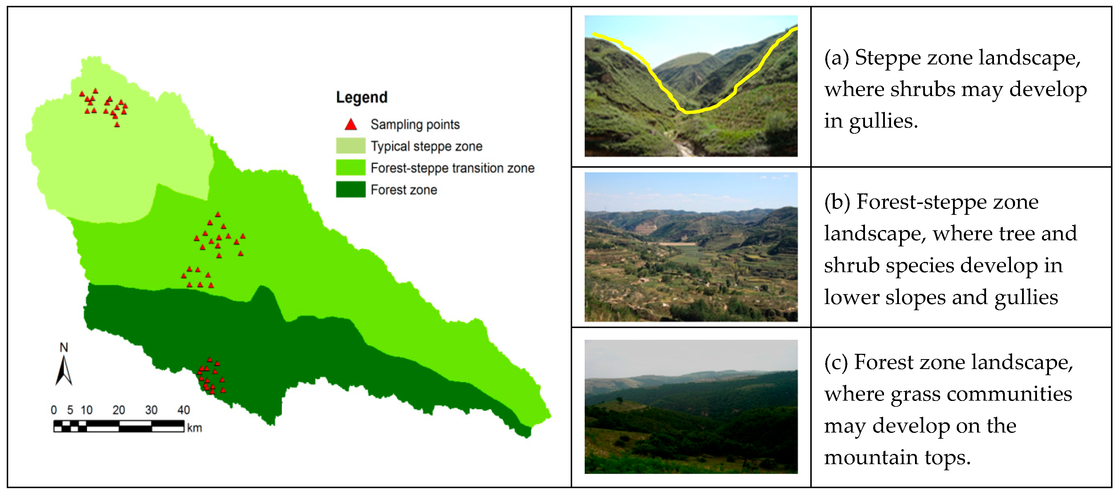
Figure 1.
Distribution of sample plots in study area and landscape of different vegetation zones in the loess hilly and gully region. The yellow line in picture (a) shows a transect line.
Figure 1.
Distribution of sample plots in study area and landscape of different vegetation zones in the loess hilly and gully region. The yellow line in picture (a) shows a transect line.


Table 1.
Estimated variance components of the plant community functional traits in the Yanhe River watershed among nine transects.
Table 1.
Estimated variance components of the plant community functional traits in the Yanhe River watershed among nine transects.
| Trait Variables | Variance Components | Statistical Parameters | |||
|---|---|---|---|---|---|
| Transect | Plot | ICC | LRatio | p | |
| LT | 0.0003 | 0.002 | 14.17% | 28.72 | <0.001 *** |
| SLA | 150.6 | 376.1 | 28.59% | 16.31 | <0.001 *** |
| LTD | 0.024 | 0.227 | 9.69% | 14.43 | <0.001 *** |
| LCC | 459 | 4289 | 9.67% | 56.96 | <0.001 *** |
| LNC | 4.016 | 21.429 | 15.78% | 22.90 | <0.001 *** |
| LPC | 0.005 | 0.121 | 4.24% | 40.27 | 0.027 |
ICC is intra-class correlation coefficient, LRatio is the likelihood ratio test for the variance, *** p < 0.001 means that there is highly significant intercept variation between transects.
Table 2.
Multilevel models of leaf traits coupled with environmental factors at different spatial scales using the restricted maximum likelihood (REML) method.
Table 2.
Multilevel models of leaf traits coupled with environmental factors at different spatial scales using the restricted maximum likelihood (REML) method.
| Parameter | LT | SLA | LTD | LCC | LNC |
|---|---|---|---|---|---|
| Fixed effects | |||||
| Intercept | 0.553 *** | 20.092 ** | 6.476 *** | 1053.81 *** | −1.491 * |
| Pa | −0.001*** | - | −0.011 *** | −0.787 ** | 0.022 * |
| SWC | −0.004 * | - | −0.070 *** | - | - |
| SOM | - | 1.175 *** | - | - | 0.141 ** |
| aspect | −0.097 *** | 50.350 *** | −1.643 *** | - | 9.126 *** |
| elevation | - | - | - | 0.153 * | - |
| Variance components | |||||
| (transect scale) | 0.0001 | - | 0.022 | 186.9 | 1.365 |
| (site scale) | 0.001 | 70.813 | 0.056 | 4215.6 | 11.480 |
| % Explained variance (transect scale) | 36.08% | - | 10.91% | 57.25% | 66.01% |
| % Explained variance (site scale) | 43.60% | 81.17% | 75.39% | 7.28% | 46.43% |
| Metrics of model support | |||||
| AIC | −1053.8 | 1889.6 | 18.01 | 2865.8 | 1372.4 |
| BIC | −1025.4 | 1925.6 | 39.26 | 2883.5 | 1400.8 |
| −2LL | 534.9 | −934.8 | −3.004 | −1427.9 | −678.2 |
*** p < 0.001, ** p < 0.01, * p < 0.05. LT—leaf thickness; SLA—specific leaf area; LTD—leaf tissue density; LCC—leaf carbon concentration; LNC—leaf nitrogen concentration; LPC—leaf phosphorus concentration. Pa—mean annual rainfall; SWC—soil water content; SOM—soil organic matter.
Table 3.
The spatial distribution pattern of leaf traits among nine transects in Yanhe River catchment.
Table 3.
The spatial distribution pattern of leaf traits among nine transects in Yanhe River catchment.
| Vegetation Zone | Transects | LT/mm | SLA/cm2·g−1 | LTD/g·cm−3 | LCC/g·kg−1 | LNC/g·kg−1 | LPC/g·kg−1 |
|---|---|---|---|---|---|---|---|
| Steppe | LJW | 0.189 ± 0.005 c | 53.819 ± 3.098 a | 1.019 ± 0.101 bcd | 510.914 ± 6.772 c | 14.377 ± 0.816 a | 1.285 ± 0.028 a |
| HZL | 0.181 ± 0.005 bc | 55.216 ± 2.853 ab | 1.162 ± 0.098 d | 470.513 ± 11.703 abc | 15.509 ± 0.789 ab | 1.378 ± 0.067 ab | |
| LDW | 0.181 ± 0.007 bc | 57.436 ± 2.965 abc | 1.091 ± 0.082 cd | 497.615 ± 13.335 bc | 14.671 ± 0.547 ab | 1.327 ± 0.059 ab | |
| Forest-steppe | HS | 0.162 ± 0.008 ab | 66.831 ± 3.691 bcd | 0.777 ± 0.073 ab | 464.819 ± 5.314 ab | 17.518 ± 0.764 b | 1.408 ± 0.068 ab |
| WLW | 0.182 ± 0.008 bc | 64.109 ± 2.826 abcd | 0.835 ± 0.089 abc | 471.467 ± 8.786 abc | 15.846 ± 0.780 ab | 1.458 ± 0.074 abc | |
| ZFG | 0.151 ± 0.007 a | 68.227 ± 3.932 cd | 0.757 ± 0.055 ab | 503.799 ± 13.842 bc | 17.650 ± 0.834 b | 1.407 ± 0.069 ab | |
| Forest | ZJT | 0.140 ± 0.007 a | 82.950 ± 3.034 e | 0.694 ± 0.103 a | 433.495 ± 18.952 a | 17.352 ± 0.766 b | 1.522 ± 0.036 bc |
| TQY | 0.148 ± 0.009 a | 85.069 ± 7.616 e | 0.645 ± 0.053 a | 455.802 ± 25.257 a | 22.081 ± 1.585 c | 1.660 ± 0.062 c | |
| MBZ | 0.163 ± 0.007 ab | 75.624 ± 3.557 de | 0.818 ± 0.104 abc | 453.426 ± 17.211 a | 17.628 ± 1.508 b | 1.490 ± 0.050 abc | |
| F-Value | 5.327 ** | 7.566 ** | 4.003 ** | 3.783 ** | 5.280 ** | 2.208 |
Note: abbreviated names in the second column are the names of near villages where transect located; LT—leaf thickness; SLA—specific leaf area; LTD—leaf tissue density; LCC—leaf carbon concentration; LNC—leaf nitrogen concentration; LPC—leaf phosphorus concentration. The means with the different letter denote a significant difference among transects at the p < 0.05 level; ** p < 0.01.
© 2018 by the authors. Licensee MDPI, Basel, Switzerland. This article is an open access article distributed under the terms and conditions of the Creative Commons Attribution (CC BY) license (http://creativecommons.org/licenses/by/4.0/).
Share and Cite
MDPI and ACS Style
Shi, H.; Wen, Z.; Guo, M. Leaf Trait Variation with Environmental Factors at Different Spatial Scales: A Multilevel Analysis Across a Forest-Steppe Transition. Forests 2018, 9, 122. https://doi.org/10.3390/f9030122
AMA Style
Shi H, Wen Z, Guo M. Leaf Trait Variation with Environmental Factors at Different Spatial Scales: A Multilevel Analysis Across a Forest-Steppe Transition. Forests. 2018; 9(3):122. https://doi.org/10.3390/f9030122
Chicago/Turabian StyleShi, Haijing, Zhongming Wen, and Minghang Guo. 2018. "Leaf Trait Variation with Environmental Factors at Different Spatial Scales: A Multilevel Analysis Across a Forest-Steppe Transition" Forests 9, no. 3: 122. https://doi.org/10.3390/f9030122
Note that from the first issue of 2016, this journal uses article numbers instead of page numbers. See further details here.