Decadal-Scale Reduction in Forest Net Ecosystem Production Following Insect Defoliation Contrasts with Short-Term Impacts of Prescribed Fires

Clark, Kenneth L.; Renninger, Heidi J.; Skowronski, Nicholas; Gallagher, Michael; Schäfer, Karina V. R.

doi:10.3390/f9030145

Open AccessArticle

Decadal-Scale Reduction in Forest Net Ecosystem Production Following Insect Defoliation Contrasts with Short-Term Impacts of Prescribed Fires

¹

Silas Little Experimental Forest, USDA Forest Service, 501 Four Mile Road, New Lisbon, NJ 08064, USA

²

Department of Forestry, Mississippi State University, Box 9681, Starkville, MS 39762, USA

³

Northern Research Station, USDA Forest Service, 180 Canfield St., Morgantown, WV 26505, USA

⁴

Department of Biological Sciences, Rutgers University, 195 University Ave., Newark, NJ 07102, USA

^*

Author to whom correspondence should be addressed.

Forests 2018, 9(3), 145; https://doi.org/10.3390/f9030145

Submission received: 25 February 2018 / Revised: 11 March 2018 / Accepted: 11 March 2018 / Published: 16 March 2018

(This article belongs to the Special Issue Forest Structural Dynamics in the 21st Century)

Download

Browse Figures

Versions Notes

Abstract

:

Understanding processes underlying forest carbon dynamics is essential for accurately predicting the outcomes of non-stand-replacing disturbance in intermediate-age forests. We quantified net ecosystem production (NEP), aboveground net primary production (ANPP), and the dynamics of major carbon (C) pools before and during the decade following invasive insect defoliation and prescribed fires in oak- and pine-dominated stands in the New Jersey Pinelands National Reserve, USA. Gross ecosystem production (GEP) recovered during the year following defoliation at the oak stand, but tree mortality increased standing dead and coarse woody debris, and ecosystem respiration (R_e) accounted for >97% of GEP. As a result, NEP averaged only 22% of pre-disturbance values during the decade following defoliation. At the pine stand, GEP also recovered to pre-disturbance values during the year following understory defoliation by gypsy moth and two prescribed fires, while R_e was nearly unaffected. Overall, defoliation and tree mortality at the oak stand drove a decadal-scale reduction in NEP that was twofold greater in magnitude than C losses associated with prescribed fires at the pine stand. Our study documents the outcomes of different non-stand-replacing disturbances, and highlights the importance of detrital dynamics and increased R_e in long-term measurements of forest C dynamics following disturbance in intermediate-age forests.

Keywords:

forest structural dynamics; forest carbon budget; disturbance; invasive insects; fire; net ecosystem productivity; leaf area index; ecosystem respiration; coarse woody debris; detritus

1. Introduction

An understanding of processes underlying recovery following non-stand-replacing disturbance is essential for accurately predicting future carbon (C) dynamics in forest ecosystems of the eastern USA. Following extensive harvesting, conversion to agriculture or intensive forestry, and then subsequent abandonment, large areas of forest throughout the northeastern USA are currently 80–140 years old [1,2]. Since abandonment, these regenerating forests have been moderate to strong sinks for atmospheric carbon dioxide (CO₂) [3,4,5,6,7]. In the mid-Atlantic region, estimates of net primary production (NPP) and net ecosystem production (NEP) for intermediate-age forests are highest for oak–hickory forests and lowest for pine-dominated forests [8,9,10]. Overall NEP has been projected to decline slowly as forests age across the region [1,9,11,12], with productivity declining more slowly for hardwood-dominated forests than conifer-dominated forests [5,9,10]. These intermediate-age forests now experience disturbance regimes dominated by wind and ice storms, insect damage, and managed wildland fire that differ in temporal and spatial scales and intensity compared to past stand-replacing disturbance such as intensive timber management or large wildfires [6,13,14,15,16]. Following disturbance, they are also likely to have different long-term trajectories of NEP compared to patterns characterizing recovery following stand-replacing disturbances [17,18]. Syntheses of NEP estimated from eddy covariance measurements following forest harvesting or wildfires in a wide range of forest types indicate that gross ecosystem productivity (GEP) is a strong function of the recovery of leaf area [17,19]. Recently, it has been hypothesized that relatively high rates of GEP and NEP in intermediate-age forests can be maintained by frequent low-intensity disturbances which delay the onset of steady-state conditions [18,20,21]. Two primary mechanisms are thought to be involved: increased canopy heterogeneity following disturbance allows greater light penetration into the sub-canopy and results in greater light use efficiency and compensatory photosynthesis by the remaining trees, saplings, and understory vegetation [22,23,24]; and nutrients released during and following disturbance are rapidly reabsorbed by recovering vegetation, stimulating foliage production and enhancing photosynthetic rates [18,25].

The fate of increased detrital mass following non-stand-replacing disturbance in intermediate-age forests remains less clear, but potentially results in greater ecosystem respiration (R_e) by enhancing rates of heterotrophic respiration (R_h) [26,27,28,29,30]. Eddy covariance measurements of NEP from a limited number of eastern forests where tree mortality and increased standing dead and coarse woody debris (CWD) have resulted in increased R_h have either reported little effect on R_e and NEP was similar to pre-disturbance levels [30], or increased R_e and reduced NEP [27]. These results contrast somewhat with a number of studies that have documented little change to R_e and reduced soil respiration following infestations of mountain pine beetle (Dendroctonus ponderosae Hopkins) and significant tree mortality in the Rocky Mountains of the western USA [22,31,32], leading to the conclusion that these forests are more resilient to insect damage than previously predicted (e.g., [26,29]). Because few long-term measurements of NEP following non-stand-replacing disturbance in eastern forests exist to evaluate process-based models, considerable uncertainty continues to exist in our ability to accurately predict future C dynamics of forests of the mid-Atlantic region.

In this study, we quantified and contrasted the response of two intermediate-age forests to two of the predominant non-stand-replacing disturbances on the mid-Atlantic coastal plain USA: invasive insect infestations and planned wildland fires. Building upon two related studies that employed repeated light detection and ranging (LiDAR) acquisitions to demonstrate an increase in heterogeneity of canopy structure following defoliation by gypsy moth (Lymantria dispar L.) and subsequent tree mortality in an oak-dominated stand [33], and crown scorch and needle and stem consumption during a relatively intense prescribed fire in a pine-dominated stand [34,35], we evaluated two hypotheses: (1) Rapid recovery of foliage results in the maintenance of GEP and aboveground net primary productivity (ANPP) following non-stand-replacing disturbance; and (2) changes to detrital mass that occur during and following disturbance alter R_h and R_e, and thus NEP. We predicted that increased detrital mass following defoliation and tree mortality at the oak stand would increase R_h and R_e, resulting in reduced NEP, and in contrast, consumption of detritus on the forest floor during fires would reduce R_h and R_e at the pine stand, resulting in increased NEP following recovery of leaf area. We used near-continuous eddy flux and meteorological measurements to estimate NEP, GEP, and R_e before and following each disturbance [35,36,37]. We used biometric measurements made in and around permanent forest census plots to estimate leaf area and its correspondence with GEP, and to estimate ANPP. We also characterized fine litterfall and decomposition rates, as well as changes in standing dead and coarse woody debris mass to assess the correspondence of detrital dynamics with R_e and estimated R_h in each stand [27,38].

2. Materials and Methods

2.1. Site Description

Stands were located in Burlington and Ocean Counties in the Pinelands National Reserve (PNR) of southern New Jersey, USA. Oak-, mixed-, and pine- dominated stands comprise the upland forests of the PNR, many of which have regenerated naturally following cessation of timber harvesting and charcoal production towards the end of the 19th century, and severe wildfires throughout the 20th century [39,40,41]. The climate is cool temperate, with mean monthly temperatures of 0.3 and 24.3 °C in January and July, respectively (1985–2015) [42]. Mean annual precipitation is 1159 ± 156 mm (mean ± 1 standard deviation (SD)). Soils are derived from the Cohansey and Kirkwood Formations, and are sandy, coarse-grained, and have low nutrient status, cation exchange capacity, and base saturation [43]. The landscape is characterized by a relatively high frequency of wildfires and prescribed burns compared to other forest ecosystems in the northeastern US [41,44,45], with the mean annual area burned in planned fires now exceeding that burned in wildfires [46]. More recently, gypsy moth and southern pine beetle (Dendroctonus frontalis Zimmermann) have impacted upland stands throughout the PNR [36,47,48].

Two intermediate-age stands were studied: an oak-dominated stand at the Silas Little Experimental Forest (US-Slt; 39°54′56.27″ N, 74°35′44.00″ W) in Brendan Byrne State Forest, and a pitch pine (Pinus rigida Mill.)-dominated stand near the Cedar Bridge fire tower (US-Ced; 39°49′4.19″ N, 74°22′32.28″ W) in the Greenwood Wildlife Management Area, referred to below as “oak” and “pine”, respectively. The oak stand is dominated by chestnut oak (Quercus prinus L.), black oak (Q. velutina Lam.), white oak (Q. alba L.), and scarlet oak (Q. coccinea Muenchh.), with scattered shortleaf (Pinus echinata Mill.) and pitch pine. The pine stand is dominated by pitch pine, with post oak (Q. stellata Wangenh.) and scrub oaks (Q. ilicifolia Wang., Q. marlandica Muench.) in the lower canopy and understory. At the beginning of the study in 2004, dominant trees in the oak and pine stands averaged 91 and 82 years old, respectively. Both stands have ericaceous shrubs in the understory, primarily huckleberry (Gaylussacia baccata (Wangenh.) K. Koch, and G. frondosa (L.) Torr. & A. Gray ex Torr.) and blueberry (Vaccinium spp.). Sedges, mosses, and lichens are also present. Further descriptions of each stand can be found in [33,34,35,36,37,38].

Repeated scanning LiDAR acquisitions have documented reductions in canopy cover and increased canopy heterogeneity at the oak stand as a result of tree mortality and gap formation following defoliation by gypsy moth in 2007 and 2008 [33], and at the pine stand as a result of canopy scorching and needle and stem consumption during a relatively intense prescribed fire conducted in 2008 [34,35]. Both disturbances initially allowed greater light penetration to the sub-canopy and understory during the growing season, and altered stand energy partitioning, resulting in greater sensible heat and reduced latent heat fluxes [49].

2.2. Net Ecosystem Production, Ecosystem Respiration, and Gross Primary Production

Annual net ecosystem production was estimated from measurements of net ecosystem exchange of CO₂ (NEE) at each site (Equation (1)):

NEP = −NEE

(1)

NEE was measured using closed-path eddy covariance systems, profile CO₂ storage measurements, and meteorological sensors mounted on antenna towers at each site. Near-continuous measurements commenced in 2004 at the oak stand and in 2005 at the pine stand. Eddy covariance systems and data processing methods are described in [36,37,49] and in detail in Appendix A. In summary, we used the convention that negative values of NEE represented a net loss of CO₂ from the atmosphere. Half-hourly fluxes were calculated from 10 Hz flux data using EdiRE (Version 1.5.0.32, University of Edinburgh, Edinburgh, Scotland) [50], and values were rejected when instrument malfunction occurred, during measurable precipitation, or when icing occurred on the sonic anemometer sensor heads, and when friction velocity (u*) < 0.2 m s⁻¹. To estimate half-hourly NEE values when we did not have measurements, daytime NEE was modeled by fitting a rectangular hyperbola to the relationship between photosynthetically active radiation (PAR) and NEE at bi-weekly (May), monthly, or bi-monthly (January and February) intervals, and nighttime NEE was modeled by regressing half-hourly net exchange rates on air temperature during the growing season or soil temperature during the dormant season using an exponential function. Model parameters and their error terms, and Pearson’s product moment correlation coefficients for the relationships between half-hourly daytime or nighttime NEE and meteorological variables were calculated using SigmaPlot software (Version 12.5, Systat Software, Inc., San Jose, CA, USA). Continuous meteorological data and the appropriate model were then used to fill gaps for periods when fluxes were not measured, and measured and modeled values were summed to estimate annual NEP. Error in gap-filling NEE was evaluated for summer daytime data (1 June to 31 August) and all nighttime data using ±1 SE of each parameter used to model half-hourly NEE, and the maximum deviation from the mean annual NEP value for each year was reported (Table A1 and Table A2). Ecosystem respiration (R_e) was estimated using nighttime NEE and continuous half-hourly air temperature during the growing season and soil temperature during the dormant season. Error in gap-filling R_e was evaluated using ±1 SE of each parameter used to model nighttime NEE, and the maximum deviation from the mean annual R value for each year were reported (Table A1 and Table A2). Annual NEP and R_e calculated using mean parameter values were summed to estimate gross ecosystem productivity (GEP) (Equation (2)):

GEP = NEP + R_e

(2)

Annual ecosystem respiration was further partitioned into estimated autotrophic respiration (R_a) and heterotrophic respiration (R_h) (Equation (3)):

R_e = R_a + R_h

(3)

Following [17,51], we assumed that R_a was approximated as 0.55 of GEP. A high degree of energy balance closure characterized measurements at each stand (e.g., [49]). Flux data for each site are available at http://ameriflux.lbl.gov/.

2.3. Aboveground Net Primary Productivity, Net Carbon Accumulation, and Consumption During Fires

Biometric measurements made at two sets of plots around each eddy flux tower were used to estimate leaf area; aboveground net primary productivity (ANPP), the dynamics of standing dead trees and saplings, coarse woody debris, and fine litter on the forest floor, and consumption of the understory and forest floor during two prescribed fires [35]. Biometric measurements were made in and around five 201 m² census plots located randomly within a 100 m radius of each flux tower (tower plots), and in 16 (oak stand) or 12 (pine stand) census plots consisting of four 168 m² subplots patterned after USDA Forest Service Forest Inventory and Analysis (FIA) protocols, arranged in a 4 × 4, 1-km² grid centered on each flux tower (FIA-type plots; Appendix B) [2,38]. In summary, live and dead trees and saplings were measured for height and diameter at breast height (diameter at breast height (DBH); 1.37 m) annually at the tower plots and periodically at the FIA-type plots, and allometric equations were used to estimate aboveground biomass and growth increments [34,52,53]. Clip plots (1 m² area; n = 10 to 20) were used to destructively harvest understory foliage and stem biomass at the peak of the growing season around the tower plots. Litterfall was collected in traps (0.42 m² area, n = 10 at the tower plots, and n = 16 or 12 at the oak and pine FIA-type plots, respectively). Leaf area index (LAI) of canopy species was estimated from the specific leaf area of needles or leaves and litterfall measurements, and LAI of understory shrubs and scrub oaks was estimated from specific leaf area of leaves and clip plot measurements. Live tree and sapling foliage production and stem growth increments calculated from allometric equations, as well as clip plot measurements of understory foliage production and stem growth increments were used to estimate ANPP. During years when defoliation occurred, canopy foliage production was estimated from corrected litterfall measurements. Forest floor mass was collected periodically throughout the study using 1.0 m² or 0.1 m² circular frames at both sets of plots, and additional 1.0 m² destructive sampling plots (n = 10 to 20) were harvested pre- and post-fire at the pine stand in 2008 and 2013 to estimate the consumption of understory vegetation and the forest floor during prescribed burns. Coarse woody debris on the forest floor was sampled in the same plots sampled for tree and sapling biomass following United States Forest Service (USFS) Forest Inventory and Analysis protocols described in [2,27,38]. Carbon flux from snags and coarse woody debris was calculated as a function of stem size, wood density, and temperature data using equations developed in [27]. Two litterbag studies were conducted at the oak stand; one study was initiated in autumn 2004 to estimate the decomposition rates of oak leaves, pine needles, shrub foliage, and fine wood <1 cm diameter that fell at the end of the growing season, and a second study initiated in spring 2008 to estimate the decomposition rate of green oak leaf fragments that fell during gypsy moth defoliation. Net accumulation and carbon release by litter in the L horizon of the forest floor was estimated by calculating a running balance of litterfall and decomposition calculated from litterbag studies. Samples of live biomass and litter were analyzed using a C/N analyzer (Leco Carbon/Nitrogen Determinator 200-288, Leco, Inc., Saint Joseph, MI, USA) or mass loss on ignition at 550 °C to estimate C content. Biometric measurements are described in greater detail in Appendix B, and in [27,33,35,37,38].

2.4. Relationships among Gross Ecosystem Production (GEP), Ecosystem Respiration (R_e), Heterotrophic Respiration (R_h), and Biometric Measurements

To examine the hypothesis that rapid recovery of foliage results in the maintenance of GEP and ANPP following disturbance, we first evaluated the relationship between maximum seasonal LAI and annual GEP for the oak and pine stands using linear regression analyses in SigmaPlot software. Initial stem growth of oaks in the spring is typically driven by the reallocation of non-structural carbohydrates (NSC) fixed during the previous year [54,55]; thus, we compared current-year and one-year-lagged annual GEP and ANPP at each stand. The hypotheses that increased detrital mass following defoliation and tree mortality at the oak stand would increase R_h and R_e, resulting in reduced NEP, and that consumption of detritus on the forest floor during fires would reduce R_h and R_e at the pine stand, resulting in increased NEP following recovery of leaf area, were evaluated by comparing annual C release estimated from the sum of fine litter on the forest floor, snags, and CWD to R_e and estimated R_h using linear regression analyses in Sigmaplot.

3. Results

3.1. Net Ecosystem Production, Ecosystem Respiration, and Gross Ecosystem Production

Annual NEP averaged 169 and 173 g C m⁻² year⁻¹ at the oak and pine stands before disturbance, respectively (Table 1, Figure 1). Annual R_e and GEP were similar among stands, and R_e and estimated R_h averaged 89% and 34% of GEP, respectively (Figure 1 and Figure 2).

During complete defoliation of the oak stand by gypsy moth early in the growing season of 2007, half-hourly daytime NEE was very low and nighttime NEE was only weakly related to air temperature (Table A1; see [36] for details). Annual NEP was −246 g C m⁻² at the oak stand in 2007, and both annual R_e and GEP were lower than during any other year of the study, representing 68% and 46% of pre-disturbance values, respectively (Figure 1a). The ratio of R_e to GEP was greater than during any other year of the study, while estimated R_h was similar to pre-disturbance values and accounted for 80% of GEP (Figure 2). Partial defoliation of the canopy at the oak stand by gypsy moth during the growing season of 2008 coincided with relatively low rates of half-hourly NEE during the daytime, and annual R_e and GEP were 82% and 73% of pre-disturbance values. By the growing season of 2009, half-hourly daytime NEE at the oak stand had recovered to rates characterizing the pre-disturbance period, and the relationship between half-hourly nighttime NEE and air or soil temperature was stronger (Table A1). Annual GEP had recovered to values characterizing the pre-disturbance period by 2009 and averaged 1607 ± 111 g C m⁻² year⁻¹ following the period of defoliation. However, although variation in annual GEP and R_e occurred with interannual climate variability, R_e accounted for a larger proportion of GEP, averaging 98 ± 1% after 2008, and estimated R_h was 43% of GEP (Figure 1a and Figure 2; Table A1). Following the period of defoliation, the oak stand was only a weak sink for CO₂, with annual NEP averaging 37 ± 18 g C m⁻² year⁻¹ (mean ± 1 SD) from 2009 to 2016, approximately 22 ± 11% of pre-disturbance values. Over the 13 years studied at the oak stand, annual NEP averaged only 41 ± 107 g C m⁻² year⁻¹ (Table 1).

At the pine stand, reduced half-hourly daytime NEE during the growing season coincided with defoliation by gypsy moth in 2007, and following a relatively intense prescribed burn conducted in March 2008. Annual NEP was only 28% and 45% of the mean pre-disturbance value in 2007 and 2008 (not including combustion losses of 442 ± 43 g C m⁻² during the prescribed burn in 2008), respectively, and annual GEP during both years was approximately 80% of the mean value during undisturbed years (Figure 1b). In contrast to the oak stand, annual NEP at the pine stand was similar to pre-disturbance values after 2008, and averaged 185 ± 37 g C m⁻² year⁻¹, excluding 2013 when a second prescribed burn was conducted. Annual GEP was 1768 ± 100 g C m⁻² year⁻¹ after 2008, and R_e accounted for 89 ± 2% of GEP over all undisturbed years (Figure 2; Table A2). Estimated R_h was 36 ± 3% of annual GEP over all years. Annual NEP and the sum of combustion losses of C averaged 89 ± 192 g C m⁻² year⁻¹ over the study period at the pine stand, approximately twice the average value measured at the oak stand (Table 1).

3.2. Biometric Measurements, Aboveground Net Primary Productivity, and Net Carbon Accumulation

At the beginning of the study in 2004, tree and sapling density were similar at the oak and pine stands, while the oak stand had 1.2 times greater basal area and 1.9 times greater biomass (Figure 3a,b; Table A3). Total leaf area during the growing season was similar among stands before disturbance, with canopy oak foliage accounting for 80% of total LAI at the oak stand, and pine foliage accounting for 68% of total LAI at the pine stand (Figure 3c,d). Aboveground net primary productivity also was similar among stands, averaging 340 and 338 g C m⁻² year⁻¹ at the oak and pine stands, respectively (Table 1). Net C accumulation by woody stems, coarse roots, and the litter layer averaged 161 and 173 g C m⁻² year⁻¹ at oak and pine stands before disturbance, respectively (Table 1, Table A4 and Table A5).

At the oak stand, live oak tree and sapling density decreased with mortality following gypsy moth defoliation, and by the end of 2011 basal area and aboveground biomass were only 59% and 70% of values in 2007, respectively (Figure 3a; Table A4). Oak tree and sapling leaf area was reduced to near zero during complete defoliation, increased to 48% of pre-disturbance values following a second leaf out in 2007, and then averaged 64 ± 3% of total leaf area from 2009 to 2016 (Figure 3c). Leaf area of understory shrubs and scrub oaks also was reduced to near zero in 2007 during herbivory by gypsy moth, but then approximately doubled relative to pre-disturbance values in 2008 and remained stable through the end of the study in 2016. Basal area, biomass, and leaf area of pine seedlings and saplings increased as canopy gaps persisted through to the end of the study. Annual ANPP was reduced only slightly during and following years when defoliation occurred, and had recovered to pre-disturbance levels by 2011, averaging 348 ± 33 g C m⁻² year⁻¹ over all years. Green oak leaf fragments and frass accounted for a much larger proportion of fine litterfall in 2007 and 2008 at the oak stand (Figure A1), and decomposed rapidly compared to litter that fell at the end of the growing season, resulting in a negative forest floor increment in 2007 and 2008 (Figure 3e, Table A4). By 2010, total fine litter flux had returned to pre-disturbance levels, and was composed of increasing amounts of pine needle litter from regenerating pine seedlings and saplings over time. Estimated C released during decomposition of the litter layer averaged 173 ± 8 g C m⁻² year⁻¹, and was relatively stable through the study (Figure A2). In contrast, the density of snags and mass of CWD on the forest floor had increased to 7.1 and 1.4 times pre-disturbance values by 2011 in the FIA-type plots, and maximum total coarse detrital mass (snags + CWD) had reached approximately 1400 g C m⁻² by the end of 2012 at the tower plots (Figure 3e, Table A3 and Table A4). Estimated C flux from snags and CWD peaked in 2011 and 2012, and accounted for up to 6.3 ± 1.5% of R_e (Figure A2; see [27] for details). Overall, biometric measurements indicated that 650 ± 402 g C m⁻² (mean ± 1 SE) had accumulated over the 2004–2016 period at the oak stand, primarily on the forest floor (Table 1 and Table A4).

At the pine stand, pine tree density and basal area increased with sapling recruitment and biomass increment, while the density and basal area of pine and oak saplings remained nearly constant (Figure 3b; Table A5). Defoliation by gypsy moth reduced the leaf area of oak saplings and understory shrubs and scrub oaks in 2007, and crown scorching during the relatively intense prescribed burn in 2008 reduced pine tree and sapling leaf area (Figure 3d). Although a majority of the aboveground stems of shrubs and scrub oaks in the understory were killed during prescribed burns in 2008 and 2013, understory leaf area recovered rapidly and averaged 97% and 106% of pre-disturbance values by the peak of the growing season, while leaf area of oak saplings recovered relatively slowly following each burn (Figure 3d). ANPP averaged 360 ± 20 g C m⁻² year⁻¹ at the pine stand, and was lowest in 2008 during the year of the relatively intense prescribed fire (Table 1). Consumption of the forest floor and understory during prescribed fires was estimated at 442 ± 43 and 399 ± 52 g C m⁻² in 2008 and 2013, of which forest floor consumption represented 88% and 89% of the total, respectively (Figure 3f; see [34] for details). Coarse woody debris increased slightly following each prescribed burn (Figure 3f, Table A5). Overall, biometric measurements indicated that net C accumulation was driven primarily by biomass increment of trees and saplings, and totaled 1031 ± 170 g C m⁻² over the 2005–2016 period (Table 1 and Table A5). Although the two prescribed burns resulted in combined consumption loss of 841 g C m⁻², equivalent to approximately five years annual NEP at the pine stand, net accumulation of C was approximately 2.2 times the amount accumulated by the oak stand over the same period.

3.3. Relationships among GEP, R_e, R_h, and Biometric Measurements

Annual GEP was significantly related to peak LAI during the growing season at the oak stand, but only weakly related to peak LAI at the pine stand (Figure 4a,b; Table 2). Annual ANPP and GEP were significantly related at the oak stand, but only weakly related at the pine stand (Table 2). Ecosystem respiration and estimated R_h were significantly related to C fluxes calculated from the sum of snags, CWD, and the forest floor at the oak stand (Figure 4c; Table 2). Despite changes to detritus on the forest floor due to consumption during prescribed burns, there was little relationship between R_e or estimated R_h and C fluxes calculated for the sum of snags, CWD, and the forest floor at the pine stand (Figure 4d; Table 2).

4. Discussion

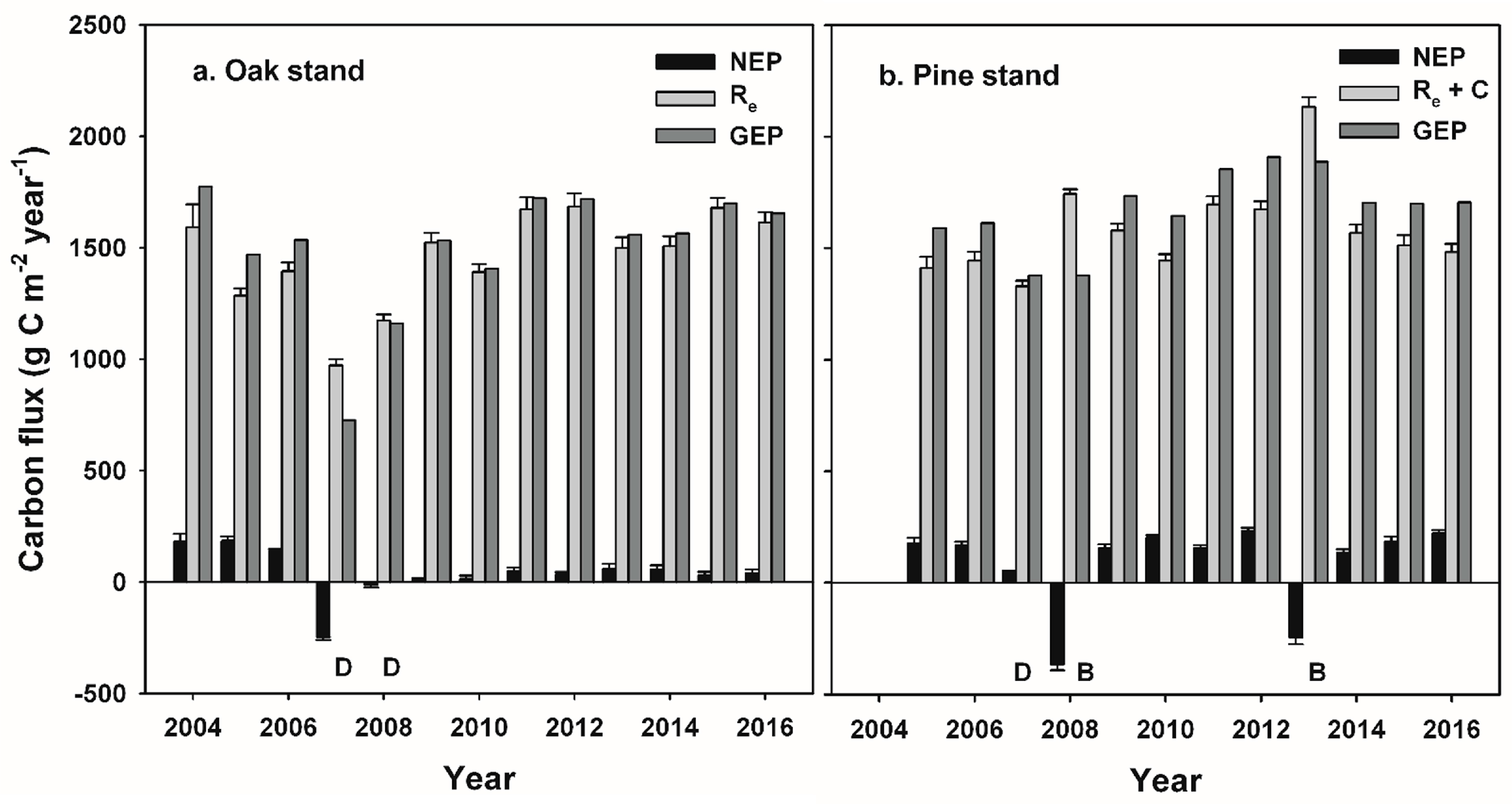
Our study indicates that infestations of defoliator insects can result in a decadal-scale reduction in NEP in oak-dominated forests of the mid-Atlantic region. In contrast, NEP following planned wildland fires in pine-dominated forests recovered to pre-disturbance values during the following year. 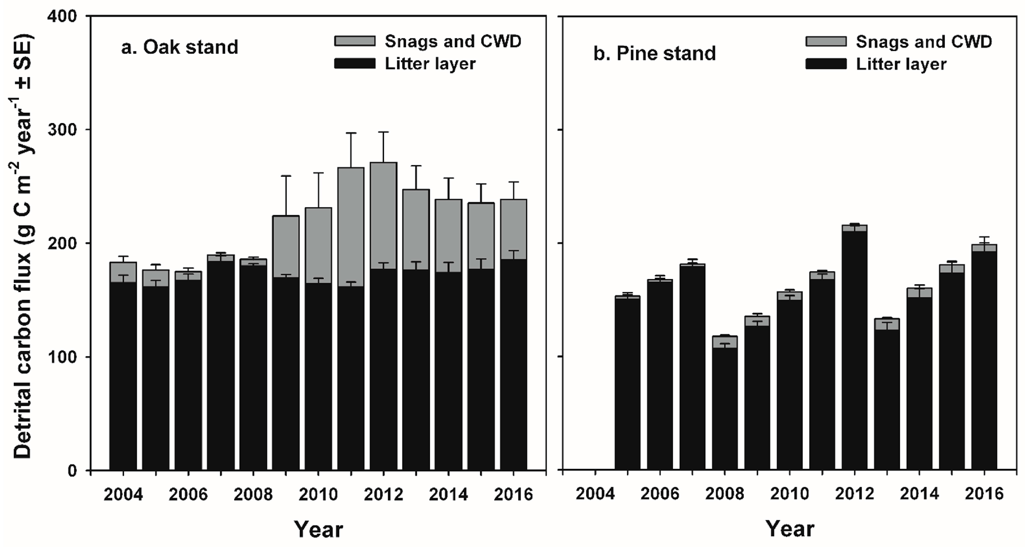Leaf area and GEP recovered rapidly following disturbance at both stands, and ANPP was nearly unaffected at both stands, consistent with patterns of recovery following non-stand-replacing disturbance in other intermediate-age forests [17,18]. 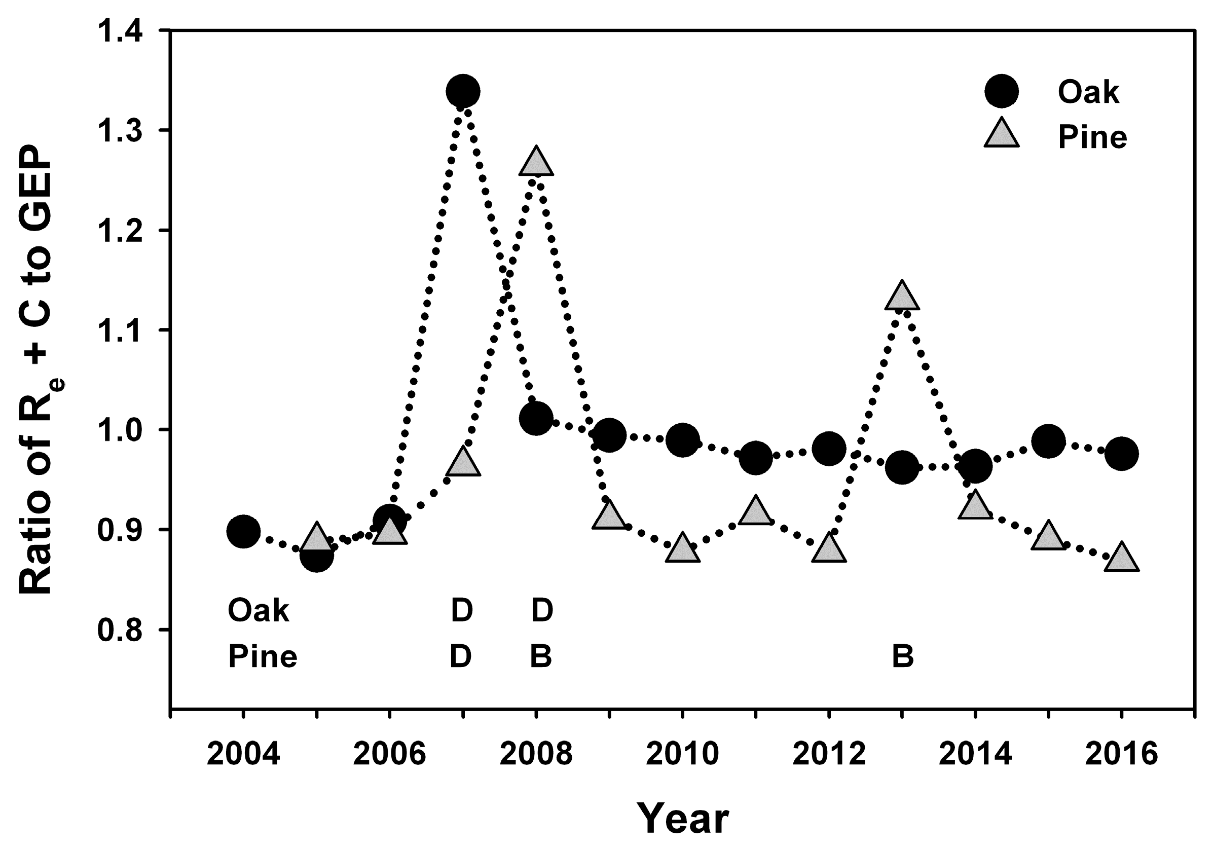At the oak stand, oak tree and sapling mortality following gypsy moth defoliation increased snag density and coarse woody debris on the forest floor, and corresponded to prolonged elevated rates of R_e and R_h, and relatively low annual NEP values during the decade following defoliation [27,30]. At the pine stand, consumption of the forest floor and understory during each prescribed burn was equivalent to annual NEP over two to three years, but had little effect on R_e or estimated R_h, and NEP was similar to pre-disturbance values in the years following each fire [35]. When integrated over multiple years, cumulative NEP and net C accumulation by major C pools indicate that patterns of recovery following these two disturbances were divergent, with annual NEP averaging only 22% of pre-disturbance values following insect defoliation, and 106% of pre-disturbance NEP values during years following prescribed burns. Divergent outcomes were related to the fate of detritus following each disturbance and its effect on R_h and R_e. Over the course of our study, the area of forest impacted by insect damage greatly exceeded that affected by wildland fires at landscape and regional scales [15,16,46,47,48]. Explicitly simulating C release from detritus following tree and sapling mortality in process-based models will lead to more accurate estimates of the magnitude of the long-term C sink in mid-Atlantic forests.

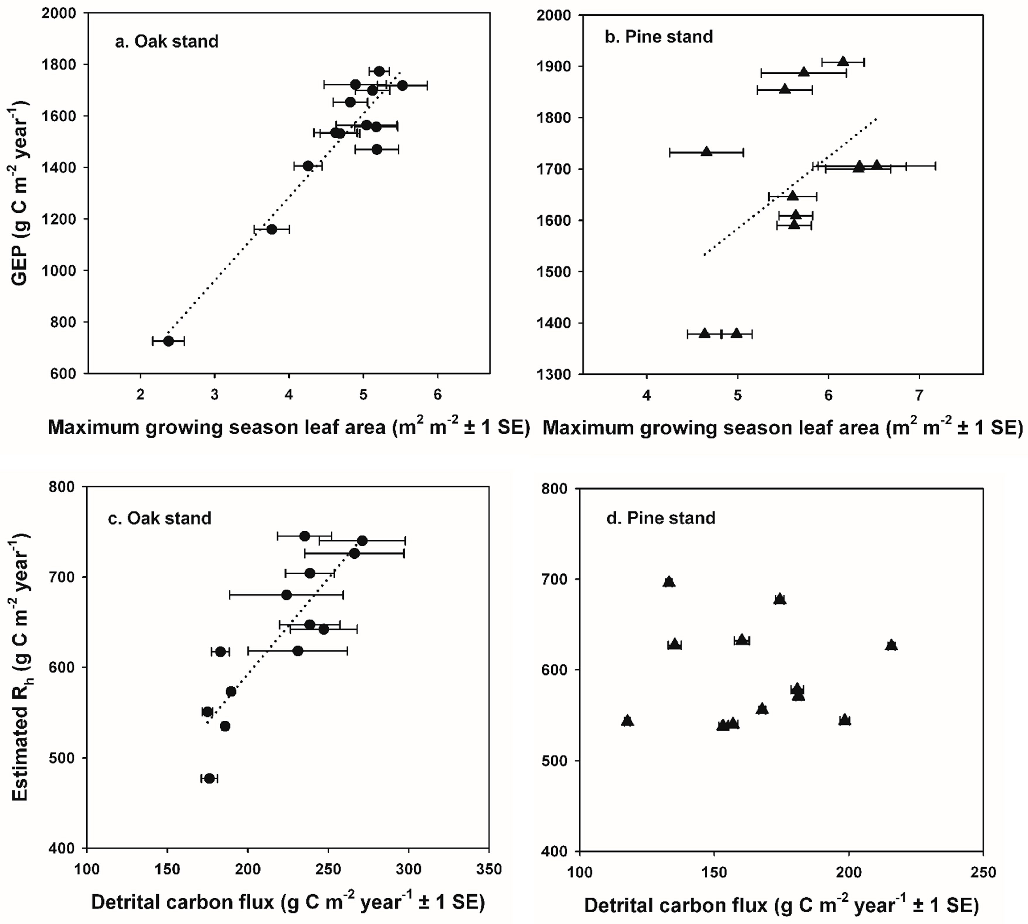
GEP returned to pre-disturbance values soon after each disturbance, corresponding to the rapid recovery of leaf area at each stand [11,17,21,54,56]. Following the cessation of herbivory or other disturbances that damage foliage early in the growing season (including experimental defoliation), canopy and understory oak species typically produce a second flush of leaves driven by the reallocation of nonstructural stored carbon (NSC) [36,37,54,55]. In late spring in 2007 at the oak stand, the second leaf flush following complete defoliation totaled approximately half of spring leaf production and had a lower mean nitrogen content than pre- or post- disturbance periods (1.7% vs. 1.9% nitrogen (N) in canopy foliage) [36,37,54,57]. Both pitch and shortleaf pines readily produce new shoots and needles from epicormic meristems following insect defoliation or fires [25,58]. Resprouting and recovery of ericaceous shrubs following wildland fires or other disturbance is well documented, and is facilitated by extensive belowground stems and root systems [35,59,60]. 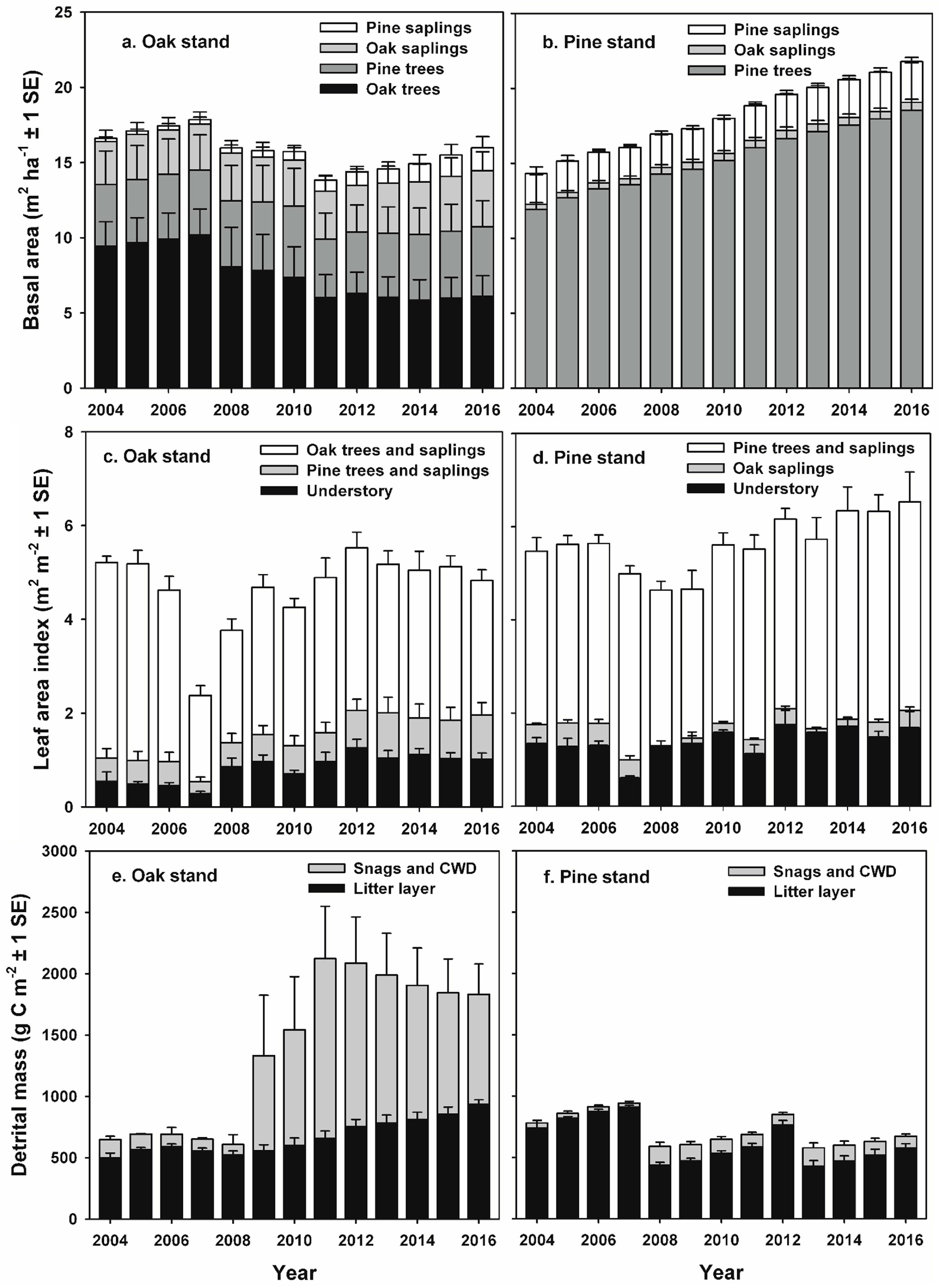Our study suggests that compensatory photosynthesis contributed to the maintenance of GEP and ANPP following disturbance [18,23]. At the oak stand, partial defoliation of the canopy in 2008 allowed greater penetration of light lower into the sub-canopy and understory, and understory shrubs and scrub oaks responded with a doubling of leaf area that was stable through the end of the study [33,37,49]. Differential mortality of black and white oaks in the canopy following defoliation resulted in large reductions in tree basal area and live biomass, and damaged individuals had reduced stem increments for up to three years following defoliation [54]. As oak mortality progressed and canopy gaps expanded, compensatory growth of undamaged canopy trees—primarily chestnut and scarlet oaks as well as pitch and shortleaf pines—were important in maintaining GEP and ANPP. Stomatal conductance and whole-tree transpiration measured using sap flux gauges increased for many of the remaining canopy oaks, suggesting that light use efficiency and photosynthetic rates also increased [23,61]. As canopy gaps persisted, increased productivity of sub-canopy oaks and pine seedlings and saplings became increasingly important in maintaining GEP and ANPP at the oak stand, similar to results reported for sub-canopy species following non-stand-replacing disturbance in other forests (e.g., [18,22,23,24,62]). Although canopy oak species in the PNR have twice the average foliar N concentrations, higher maximum stomatal conductance, and greater water use efficiencies (WUEs) compared to pitch and shortleaf pines, pines and oaks have similar light compensation points, quantum yields, and maximum assimilation rates on a leaf area basis [61]. Pines also maintain greater leaf area through the dormant season, and are photosynthetically active earlier in the spring and later in the fall compared to oaks [37,61]. 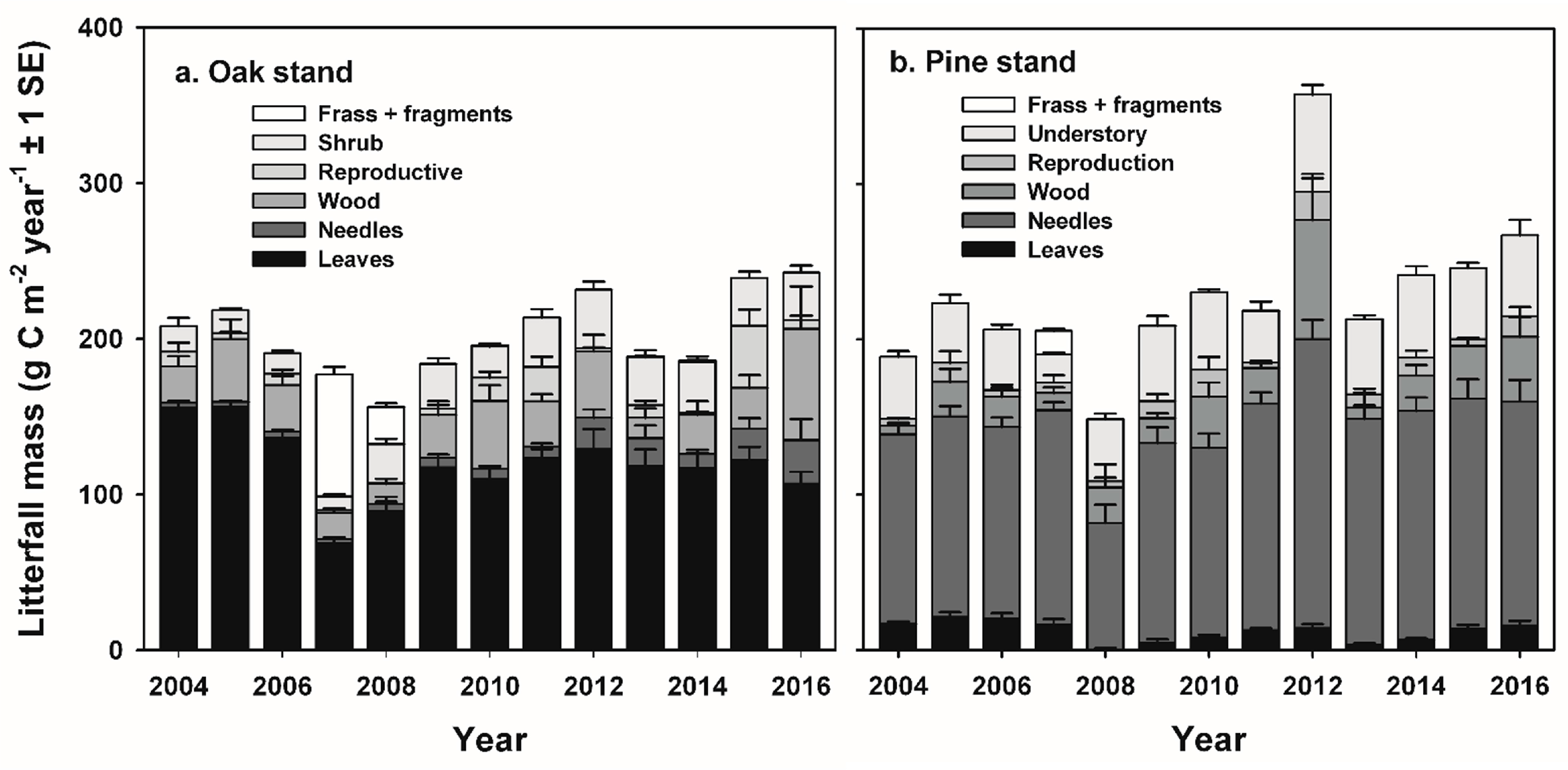At the pine stand, rapid recovery of understory foliage likely compensated for canopy foliage that was scorched and abscised prematurely during the relatively intense prescribed fire in 2008 [25,34,35]. Redistribution of nutrients released following disturbance also likely contributed to the maintenance of GEP and ANPP, with mechanisms driving nutrient redistribution related to the type of disturbance. At the oak stand, complete defoliation of the canopy and understory transferred 6.5 g N m⁻² in frass and green leaf fragments to the forest floor by mid-summer, approximately twice the amount of N that would normally occur in litterfall during the fall months [36,37]. Canopy foliar N concentrations and total N content were lower in the second flush of foliage following defoliation, and ecosystem WUE was reduced by approximately 42% during the growing season compared to pre-disturbance years [37,57]. During the growing seasons following insect defoliation, little difference in foliar N levels or assimilation rates of canopy oak foliage occurred, but overall canopy N content was lower following oak mortality compared to the pre-disturbance period [61,63]. However, foliar N content of sub-canopy and understory species increased following defoliation, and thus little net change in the total amount of N in foliage occurred and ecosystem WUE was not significantly different pre- and post-disturbance [37,57,63]. Increased foliar N levels and enhanced maximum assimilation rates in the remaining pine needles were observed following relatively intense prescribed burns in the PNR, but not during low-intensity burns [25,64]. Increased N levels and photosynthetic rates following wildland fires are likely related to the transient pulse of inorganic N associated with consumption of forest floor material, in addition to pyro-mineralization and release of phosphorus and basic cations [65,66]. Enhanced photosynthetic rates in pine needles did not persist beyond the first growing season following each fire [25,64].

Non-stand-replacing disturbances can initially lead to reduced R_e, R_a and soil respiration, because reduction in leaf area and canopy photosynthesis results in reduced C supply to fine roots and the rhizosphere [22,32,67,68], and alters the allocation of NSC to storage pools [54,55]. Simultaneously, an increase or decrease in detrital pools can occur, and respiration of previously-fixed C can lead to increased R_h [27,28,29,30,69]. The initial reduction in R_e during defoliation by gypsy moth in 2007 and 2008 at the oak stand is consistent with patterns of reduced R_e and soil CO₂ flux reported following mortality by mountain pine beetle in the Rocky Mountains of the western USA [22,31,32,68], and with girdling treatments in a variety of forests (e.g., [67,70,71]). Although we lack long-term measurements of soil respiration, fine root productivity, and changes in O horizon and soil C pools, estimated partitioning of R_e following [17,51] indicates that R_a was relatively small in magnitude while R_h was similar to pre-disturbance values, suggesting that the supply of labile C to fine roots and associated mycorrhizal fungi in the rhizosphere was limited during and immediately following insect defoliation at the oak stand.

The reduction in R_e that we observed was relatively short-lived and limited to the two years when defoliation occurred at the oak stand, and the transition to increased R_h occurred during the year following defoliation, as mortality of oak trees and saplings increased standing dead and forest floor detritus. Our results are consistent with experimental girdling treatments in an intermediate-age oak-dominated forest in New York, USA that resulted in a 50% mortality of red (Quercus rubra L.), black, white, and chestnut oaks, where soil respiration returned to pre-disturbance levels after two years [71]. At the oak stand, estimated respiration from additional snags and CWD ≥ 7 cm diameter in the FIA-type plots contributed 30 g C m⁻² year⁻¹ and 46 g C m⁻² year⁻¹ to annual R_e at the oak stand in 2009 and 2011, representing approximately 2 and 4% of R_e, and 18% and 27% of pre-disturbance NEP values, respectively [27]. Our estimates of C fluxes from CWD are somewhat higher (up to 7% of R_e and 68% of pre-disturbance NEP) than those reported in [27] because we estimated CO₂ fluxes from smaller-diameter stems, and tree mortality continued through 2012. The increase in respiration from detritus following non stand-replacing disturbance is consistent with experimental girdling and overstory mortality in an intermediate-age aspen (Populus gradidentata Michaux) and birch (Betula papyrifera Marshall) stand that resulted in an increase of approximately 3500 g C m⁻² as snags and CWD, which enhanced R_h from snags and CWD from 110 to 210 g C m⁻² year⁻¹, and accounted for 12 to 24% of R_e six years following girdling [30]. In the long-term, our results contrast with the persistent reduction in R_e and soil respiration reported following stand damage by mountain pine beetle [22,31,32,68], and in girdling experiments documented in [21,30]. Much of the insect damage in oak-dominated forests in the PNR resulted in mortality of <40% of canopy trees, and not to the extent of canopy tree mortality observed in stands impacted by mountain pine beetle (40% to >80% mortality) [13,22,26,72] or of southern pine beetle in the PNR (>90% pine mortality) [47]. In comparison to other stands impacted by insect infestations, a threshold likely exists where low levels of mortality are insufficient to reduce components of R_e—including respiration from live fine roots and mycorrhizal fungi in the rhizosphere—for long periods of time, but still severe enough to increase detrital mass and R_h [27,30,73]. Enhanced dynamics of snags and CWD in our study are also likely related to climatic differences, as CO₂ release from detritus had a strong temperature dependence early in the decomposition process, with r² values of 0.59 and 0.81 for the relationship between substrate temperature and CO₂ emissions for standing dead and CWD, respectively [27], as well as the presence of abundant fungal decomposers [74] and macroinvertebrates such as termites in the PNR.

Our study indicates that infestations of defoliating insects will have significant consequences for the NEP of oak-dominated forests at landscape to regional scales in the future. We previously used aerial survey data to estimate that severe gypsy moth defoliation of approximately 20% of the upland oak-, mixed, and pine-dominated stands in the 400,000 ha Pinelands National Reserve in 2007 reduced landscape-scale NEP by approximately 41% [36,75]. During the course of our study (2004–2016), moderate-to-severe defoliation and tree mortality caused by gypsy moth totaled 503,000 ha, and damage by southern pine beetle resulting in >90% pine tree mortality totaled 19,550 ha in New Jersey alone, equivalent to approximately 65% of the forested area in the state [46,47,76]. The proportion of forest area impacted by insects in New Jersey during some years of our study exceeded 12% year⁻¹, one of the highest rates of forest disturbance in the mid-Atlantic or northeastern USA, which averaged 2 to 4% year⁻¹ over the same period [15,16,76].

Aerial surveys and remotely sensed information derived from Landsat, MODIS, and other satellite products are highly effective at detecting changes in leaf area resulting from insect defoliation or wildland fire [8,15,16,45,76]. However, changes in tree and sapling biomass, and the increase in standing dead and CWD that we quantified using a much denser network of FIA-type forest inventory plots that was sampled more frequently than standard FIA plots distributed across the region are more difficult to detect remotely. Repeated LiDAR acquisitions have successfully detected changes in canopy and sub-canopy biomass following insect defoliation and tree mortality as well as wildland fires, but accurately sampling changes in detrital mass on the forest floor is more difficult [33,34,71]. Similarly, predicting the impact of invasive insects on long-term forest C dynamics using process-based simulation models has been only partially successful. Although process-based models have accurately captured the effects of gypsy moth defoliation on tree biomass, stand species composition, and the dynamics of GEP and ANPP, they have generally underestimated the long-term reduction in NEP in forests of the PNR following disturbance [9,10,11]. For example, the Ecosystem Demography 2 Model parameterized for xeric hardwoods and conifers and to represent defoliation events and tree mortality at oak-dominated stands in the PNR over 200-year simulations indicated that defoliation intensity was linearly related to decreases in annual NEP, but also predicted that post-disturbance NEP exceeded 80 to 90 g C m⁻² year⁻¹ at all levels of defoliation [11]. Simulations with LANDIS II coupled with the CENTURY succession extension [10] predicted changes in species composition and reduced live tree biomass accurately in the PNR, but also predicted relatively little effect on long-term NEP following periodic gypsy moth outbreaks over 100-year simulations [10]. Neither of these models accurately capture the dynamics of detritus resulting from tree and sapling mortality, which our study demonstrates is important in the decadal-scale reduction in NEP. More recently, parameterization of PnET-CN [12]) using extensive forest inventory data and tree mortality rates to explicitly simulate wood turnover in mid-Atlantic forests where oak mortality was significant resulted in relatively low estimates of annual NEP that are similar in magnitude to those measured in our study [12,77].

In comparison to insect damage, wildfires and prescribed burns have disturbed much less area in New Jersey, with 36,656 ha affected by wildfires and 76,829 ha affected by prescribed burning over the course of our study [45,78]. Consumption of the forest floor and understory across a range of prescribed burns conducted in oak-, mixed-, and pine- dominated forests is equivalent to approximately two to four years annual NEP [35], but prescribed fires apparently have little effect on the ratio of GEP to R_e or to estimated R_h, in contrast to simulations using BiomBGC (Terrestrial Ecosystem Process Model) [19] that predicted litter consumption by prescribed fires would reduce R_h and increase NEP (e.g., [79,80]). Future improvements to process-based models simulating forest carbon cycling and the impacts of insects and wildland fires should focus on a better representation of the dynamics of snags, CWD, and the forest floor following disturbance, such as the approach employed by [12].

Forests in the mid-Atlantic and northeastern USA are exposed to a relatively large and increasing number of invasive insects and pathogens that can result in increased rates of tree and sapling mortality, including gypsy moth, southern pine beetle, emerald ash borer (Agrilus planipennis), hemlock wooly adelgid (Adelges tsugae), and spruce budworm (Choristoneura spp.) [13,14,15,16,47,48,81]. If our results can be extended to intermediate-age forests across these regions that will be impacted by insect damage in the future, the potential for long-term reductions in NEP dwarfs C losses from all other disturbances other than forest harvesting [15,16,81]. Accurately detecting and accounting for the impacts of invasive and native insects on rates of tree mortality and enhanced losses of C via respiratory pathways in process-based simulation models will greatly improve our estimates of the magnitude of the long-term CO₂ sink in forests in the mid-Atlantic and northeastern USA.

5. Conclusions

Our study supports the hypothesis that GEP and ANPP are maintained following non-stand-replacing disturbance in intermediate-age forests. However, our results contrast with some recent observations that insect damage does not have significant consequences for forest carbon dynamics. Prolonged enhanced rates of R_e and R_h were related to increased detritus following tree and sapling mortality, and resulted in a decadal-scale reduction in NEP. Because the maintenance of high rates of NEP following non-stand-replacing disturbance is dependent upon the fate of detritus and its effect on R_h, remote sensing products and simulation models that explicitly account for changes in detrital mass will likely provide more accurate estimates of long-term forest carbon dynamics of intermediate-age stands following disturbance.

Acknowledgments

This research was supported in part by a grant from the National Aeronautical and Space Agency (NNH08AH971), USDA Joint Venture Agreement 10-JV-11242306-136, and the National Fire Plan. All of the eddy covariance and meteorological data used in this manuscript are available at the Ameriflux website (http://ameriflux.lbl.gov/; the oak stand is US-Slt and the pine stand is US-Ced). The biometric data is available through USDA Forest Service websites, with links published in [38].

Author Contributions

K.L.C. and N.S. conceived and designed the field sites; K.L.C., H.J.R., N.S., M.G. and K.V.R.S. collected all field data; K.L.C. and H.J.R. analyzed the data; N.S. and M.G. contributed LiDAR analytical tools; K.L.C., H.J.R. and K.V.R.S. wrote the paper.

Conflicts of Interest

The authors declare no conflict of interest in all aspects of this study.

Appendix A

Eddy Covariance and Meteorological Measurements

Eddy covariance and continuous meteorological measurements were used to estimate net ecosystem exchange of CO₂ (NEE), net ecosystem production (NEP), ecosystem respiration (R_e), and gross ecosystem production (GEP) at the oak and pine stands. Eddy covariance systems were composed of a three-dimensional sonic anemometer (RM 80001V, R. M. Young, Inc., Traverse City, MI, USA), a closed-path infrared gas analyzer (IRGA; LI-7000, LI-COR Inc., Lincoln, NE, USA), a 0.4 cm internal diameter Teflon-coated tube and an air pump, and a laptop computer [36,49]. The sonic anemometer was mounted approximately 4 m above the canopy at each site, with the inlet of the air sampling tube attached between the upper and lower sensors of the sonic anemometer. Air was drawn through the sample channel of the IRGAs at a rate of 6.0 to 8.0 L min⁻¹, resulting in a lag time of approximately 2.0 s. N₂ scrubbed with soda lime and magnesium perchlorate was used as a blank in the reference channel at a rate of 0.2 L min⁻¹, and to zero the IRGAs. The IRGAs were periodically calibrated for CO₂ using CO₂ calibration tanks that were traceable to primary standards, and for water vapor using a dew point generator (LI-610, LI-COR Inc.) or a sling psychrometer. Coordinate rotation of the raw sonic anemometer signals was used to obtain turbulence statistics perpendicular to the local streamline. The maximum values for the covariance between turbulence and CO₂ concentrations were used to calculate half-hourly values of NEE. We used the convention that negative values of NEE represented a net loss of CO₂ from the atmosphere. Fluxes were corrected for frequency attenuation of scalar concentrations down the sampling tube and non-ideal frequency response of the IRGAs using transfer functions in EdiRE [50]. Barometric pressure data was then used to calculate half-hourly fluxes at ambient atmospheric pressure. A three-step filter was used to remove spikes and poor-quality half-hourly data: (1) Periods when instruments failed or the IRGA was out of calibration were first removed. (2) Data when precipitation occurred or ice formed on the sonic anemometers were then removed. (3) We then applied a friction velocity (u*) filter to the remaining half-hourly values. Nighttime NEE values at 2 °C bins converged on stable values at a u* value of approximately 0.2 m s⁻¹, and we removed all half-hourly NEE data below this u* value (Table A1 and Table A2). The flux associated with the change in storage of CO₂ in the air column beneath the inlet was estimated using half-hourly top of tower concentrations and 2-m height measurements (LI-870, LI-COR Inc.), or a profile system with inlets at 2, 10, and 19 m height (oak stand during the growing season).

Daily to annual estimates of NEP require continuous values of half-hourly NEE [82]. To estimate half-hourly NEE for daytime periods when we did not have measurements (due to low windspeed conditions, precipitation, instrument failure, etc.), we fit a parabolic function (growing season) or a linear function (dormant season) to the relationship between photosynthetically active radiation (PAR) measured above-canopy and NEE at bi-weekly (May) to monthly intervals [36,37]. For nighttime periods, we fit an exponential function to the relationship between half-hourly air temperature (growing season) or soil temperature (dormant season) and NEE (Equation (A1)):

NEE = α exp (β T_air or T_soil),

(A1)

where exp is the exponential function, T_air is half-hourly mean above-canopy air temperature, and T_soil is half-hourly mean soil temperature at 5 cm depth.

Coefficients for gap filling were calculated from data collected during the appropriate time periods using SigmaPlot regression software (Systat Software, Inc., San Jose, CA, USA). Continuous meteorological data and the appropriate model were then used to fill gaps for periods when fluxes were not measured. Annual NEP was calculated by summing measured and modeled half-hourly values. We used ±1 SE of each parameter in the parabolic function for daytime data during the summer (1 June to 31 August) when peak NEE occurred, and in the exponential function for all nighttime data to evaluate the sensitivity of annual NEP estimates to modeled values we used in gap-filling (Table A1 and Table A2). Ecosystem respiration (R_e) was estimated for each stand using continuous half-hourly air temperature during the growing season and soil temperature during the dormant season. Error in gap-filling R_e was evaluated using ±1 SE of mean parameter values used to calculate annual R_e, and the maximum deviation from the mean annual R_e value was reported (Table A1 and Table A2). Annual NEP and R_e calculated using mean parameter values were summed to estimate gross ecosystem productivity (GEP).

Continuous meteorological measurements were made at each flux tower. Incoming shortwave radiation (LI-200, LI-COR, Inc.), photosynthetically active radiation (PAR; LI-190, LI-COR, Inc.), net radiation (NRLite, Kipp and Zonen, Inc., Delft, the Netherlands), air temperature and relative humidity (HMP45c, Vaisala, Inc., Woburn, MA, USA), windspeed and direction (05013-5, R. M. Young Co.), and precipitation (TE525, Texas Electronics, Inc., Dallas, TX, USA) were measured above each canopy. Soil heat flux was measured using heat flux transducers (#HFT-3.1, Radiation and Energy Balance Systems, Inc., Seattle, WA, USA) buried at 10 cm depth within 10 m of the tower at each site, and soil temperature was measured at 5 cm depth (CS-107, Campbell Scientific, Inc., Logan, UT, USA) at each site. Barometric pressure (PTB 100A, Vaisala, Inc., Vantaa, Finland) was measured from the tower at the oak stand. Meteorological data were recorded with automated data loggers (CR23x, CR1000, Campbell Scientific, Inc., North Logan, UT, USA). Eddy covariance and meteorological measurements are further detailed in [36,37,48].

Table A1. Annual net ecosystem production (NEP), ecosystem respiration (R_e), and information for half-hourly nighttime net ecosystem exchange of CO₂ (NEE) derived from eddy covariance measurements at the oak stand. Values in parentheses for NEP are the maximum deviations from annual values as a result of gap filling using ±1 SE parameter values derived from daytime data during the summer (1 June to 31 August) or all nighttime data, and values in parentheses for R_e are the maximum deviation from annual values as a result of gap filling using ±1 SE of parameter values derived from all nighttime data. The number of half-hourly values when u* ≥ 0.2 m s⁻¹, Pearson’s product moment correlation coefficients for the modeled relationship between air or soil temperature, and temperature coefficients for air (Q_{10 air}) and soil (Q_{10 soil}) temperature for 10 to 20 °C are shown. * indicates years when disturbance occurred.

Year	NEP	R_e	Nighttime Half-Hourly NEE
g C m⁻² year⁻¹			n	Air Temperature		Soil Temperature
				r²	Q_{10 air}		r²	Q_{10 soil}
2004	181 (35)	1592 (103)	1706	0.432	2.14		0.402	2.70
2005	185 (20)	1285 (33)	3078	0.434	1.88		0.444	2.24
2006	140 (16)	1395 (39)	3353	0.446	2.11		0.489	2.49
2007 *	−246 (14)	972 (28)	3500	0.285	1.66		0.284	1.89
2008 *	−13 (11)	1173 (28)	3637	0.370	1.72		0.402	2.05
2009	9 (10)	1523 (44)	3669	0.493	2.25		0.565	2.92
2010	15 (14)	1391 (35)	3952	0.387	1.66		0.373	1.95
2011	49 (16)	1673 (54)	3680	0.409	2.06		0.493	2.76
2012	33 (12)	1685 (59)	3523	0.437	2.30		0.528	3.06
2013	59 (22)	1499 (48)	2984	0.533	2.25		0.544	2.79
2014	57 (18)	1507 (44)	3505	0.447	2.08		0.518	2.76
2015	30 (16)	1679 (45)	3516	0.387	1.87		0.398	2.21
2016	40 (17)	1614 (46)	3336	0.361	1.83		0.404	2.25

Table A2. Annual net ecosystem production (NEP), the sum of ecosystem respiration and combustion loss during prescribed fires (R_e + C), and information for half-hourly nighttime net ecosystem exchange of CO₂ (NEE) derived from eddy covariance and biometric measurements at the pine stand. Values in parentheses for NEP are the maximum deviations from annual values as a result of gap filling using ±1 SE of parameter values derived from daytime data during the summer (1 June to 31 August) or all nighttime data, and values in parentheses for R_e + C are the maximum deviation from annual values as a result of gap filling using ±1 SE of parameter values derived from all nighttime data. The number of half-hourly values when u* ≥ 0.2 m s⁻¹, Pearson’s product moment correlation coefficients for the modeled relationship between air or soil temperature, and temperature coefficients for air (Q_{10 air}) and soil (Q_{10 soil}) temperature for 10 to 20 °C are shown. * indicates years when disturbance occurred.

Year	NEP	R_e + C	Nighttime Half-Hourly NEE
	g C m⁻² year⁻¹		n	Air Temperature		Soil Temperature
				r²	Q_{10 air}	r²	Q_{10 soil}
2005	178 (24)	1412 (49)	1353	0.522	1.82	0.565	2.26
2006	168 (12)	1441 (32)	3166	0.457	1.90	0.505	2.14
2007 *	49 (7)	1329 (26)	4007	0.476	1.77	0.490	2.05
2008 *	−365 (26)	1743 (22)	4080	0.434	1.76	0.458	1.95
2009	152 (18)	1580 (30)	3668	0.587	2.09	0.624	2.32
2010	201 (12)	1445 (28)	3903	0.447	1.65	0.449	1.93
2011	157 (12)	1697 (36)	3713	0.551	1.98	0.585	2.32
2012	233 (14)	1675 (36)	3880	0.509	1.99	0.547	2.58
2013 *	−246 (30)	2133 (44)	3024	0.471	1.98	0.511	2.28
2014	135 (16)	1507 (35)	3952	0.502	2.09	0.527	2.58
2015	187 (20)	1513 (46)	2949	0.427	1.79	0.384	2.39
2016	224 (14)	1482 (38)	3475	0.446	1.97	0.455	2.43

Appendix B

Biometric Measurements at Tower and Forest Inventory and Analysis (FIA)-Type Plots

Biometric measurements were made at two sets of plots around each eddy flux tower: in and around five 201 m² census plots located randomly within a 100 m radius of each flux tower (tower plots); and in 16 (oak stand) or 12 (pine stand) census plots, with each plot consisting of four 168 m² subplots patterned after USDA Forest Service Forest Inventory and Analysis (FIA) protocols [2], arranged in a 4 × 4, 1-km² grid centered on each flux tower (FIA-type plots). At the tower plots, stem diameter at 1.37 m (DBH, cm) and height (m) of all live and dead trees and saplings were measured annually, and biomass and growth increments were calculated using published allometric relationships [34,51,52]. Aboveground biomass of understory vegetation was estimated by harvesting 10 to 20 clip plots (1.0 m²) in the vicinity of each plot each year during the time of peak biomass in mid-summer. Samples were separated into stems and foliage by genus, dried at 70 °C until dry, and then weighed.

Fine litterfall was collected approximately monthly when present and bi-weekly for frass and leaf fragments during defoliation from two 0.42 m² wire mesh traps adjacent to each tower plot (n = 10 traps per stand; Figure A1). Samples were separated into leaf, needle, wood, reproductive material, frass, and green leaf fragments, dried at 70 °C, and then weighed. Specific leaf area (SLA; m² g dry weight⁻¹) for each major species was measured with a leaf area meter (LI-3000a, LI-COR Inc.) and a conveyer belt (LI-3050c, LI-COR Inc.) using fresh leaf, needle, or litterfall samples, which were then dried at 70 °C and weighed. Maximum annual canopy leaf area index (LAI; m² m⁻² ground area) was estimated for major species by multiplying litterfall mass by the appropriate SLA value and then summing results for all species. Projected leaf area of pine needle fascicles was multiplied by π to calculate an all-sided LAI (e.g., [83]). Understory LAI was estimated by multiplying dry foliage mass obtained from each clip plot by the corresponding SLA values.

Figure A1. Litterfall (g C m⁻² year⁻¹) separated by component at the (a) oak and (b) pine stands. Values are means ± 1 SE from litterfall traps near the tower plots (n = 10 for each stand).

Aboveground net primary production (ANPP) was estimated by summing the woody stem increments of live trees and saplings calculated from allometric equations, understory stem increments estimated from clip plots, and annual foliage production estimates from allometric equations and clip plots. For years when significant defoliation or prescribed burns occurred, canopy foliage production was estimated from litterfall measurements of green leaf fragments, frass, and litter corrected for mass loss at the end of the growing season [37].

Carbon in standing dead trees (snags) was estimated by recording the species, DBH, and decay class of each snag, following [27]. Decay classes were defined using FIA protocols [2,38], and were used to correct allometric equations for stem and branch dry weight based on the proportion remaining in each decay class and density of wood samples collected from trees of each species and decay class. Coarse woody debris (CWD) in each plot was estimated by measuring the small end and large end diameter, length, and decay class of all stems >7.6 cm diameter. Mass was calculated from volume and wood density, based on species-specific decay classes [27,38]. Forest floor mass was collected in two-to-five 1.0 m² circular frames in the vicinity of each plot in 2004, 2006, and 2008, and using 0.1 m² circular frames at the oak stand in 2011 and the pine stand in 2012. Additional 1 m² clip plots (n = 10 to 20) were sampled pre- and post-burn to estimate the consumption of understory shrubs, scrub oaks, saplings, and the L horizon at the pine stand in March and April 2008 and 2013. Consumption of the O horizon was minimal during the two prescribed fires conducted at the pine stand, consistent with measurements made during prescribed burns conducted during the dormant season throughout the PNR [35].

Two litterbag decomposition studies were conducted at the oak stand. In the first study, litterbags (10 cm × 20 cm, 1 mm mesh size) containing 5.0 g equivalent dry weight of pine needles, overstory oak foliage, understory oak foliage, or shrub foliage collected in the fall were used to estimate mass loss over a three-year period. Litterbags (n = 40 for each component) were placed at random locations within the vicinity of each tower plot at the oak stand, and harvested at 6, 12, 24, and 36 months. For the second litterbag study, 5.0 g equivalent dry weight of green leaf fragments of white, black, or chestnut oak collected in early June 2008 were placed in litterbags (n = 30 for each species) and harvested at 3, 6, and 12 months.

To estimate changes in mass and C release from the L horizon of the forest floor at the oak and pine stands, we used litterfall data and decay constants (k) based on litterbag studies to model the dynamics of each component. We fit an exponential decay model with the form of Equation (A2):

y = e ^{(−k × x)},

(A2)

where x is the time in years, and y is the proportion of initial mass remaining to litter decomposition data for each component [84].

Mass loss and C release from annual “cohorts” of each litter component were estimated from a running balance of litterfall amounts and decomposition rates, and were summed for all components to calculate annual net accumulation and C release from the forest floor (Figure A2, Table A4 and Table A5). To estimate mass loss and C release from snags and CWD, we calculated k constants based on mass, wood density, and CO₂ emission measurements reported in [27]. The original CO₂ flux equations were based on surface area of snags > 12.7 and CWD > 7.6 cm diameter. However, later in the decomposition process, estimating an accurate surface area was difficult due to continued fragmentation of CWD on the forest floor, and when snags fell. To reduce the uncertainties in calculating CO₂ flux using surface areas, we used an average k value of 0.073, which most closely approximated the rate of CO₂ release reported in [27].

Figure A2. Estimated annual carbon release from fine litter in the L horizon on the forest floor, standing dead, and coarse woody debris at the (a) oak and (b) pine stands.

At the FIA type plots, species, height, diameter at breast height, crown size and position, and condition were recorded for live trees and saplings in 2004, 2006, 2008, and 2010 at the oak stand, and in 2004, 2006, 2008, and 2011 at the pine stand (Table A3). Allometric equations were used to calculate tree and sapling biomass in each subplot, and then averaged within plots. Age of the dominant overstory trees at the beginning of the study was estimated from tree cores taken at 1.37 m height from the largest trees in each center subplot in 2004 and 2005. Litterfall was collected using traps (0.42 m²) located near the center of the central FIA-type plot, for a total of 16 traps at the oak stand and 12 traps at the pine stand. Samples were dried at 70 °C until dry, separated into overstory leaves, pine needles, shrub leaves, wood, reproductive material, and frass and green leaf fragments when present, and weighed. Carbon in standing dead trees was estimated by recording the species, DBH, and decay class of each snag, following [27]. Decay classes were defined using FIA protocols [2], and were used to correct allometric equations for stem and branch dry weight based on the proportion remaining in each decay class and density of wood samples collected from trees of each species and decay class (Table A3).

Forest floor mass was collected in the vicinity of all FIA-type subplots using 0.1 m² circular frames at the oak stand in 2011 and the pine stand in 2012. Samples were separated into litter (L) and organic (O) horizons, and sieved through 2 mm mesh, and then sorted into fine litter, wood, and reproductive material. Coarse woody debris (CWD) in each FIA-type subplot was estimated by measuring the small end and large end diameter, length, and decay class of all stems >7.6 cm in diameter along three transects. Mass was calculated from volume and wood density, based on species-specific decay classes [27]. Forest census data for the FIA-type plots are available at links provided in [38].

Table A3. Summary of carbon pools estimated for Forest Inventory and Analysis (FIA)-type and tower plots at the oak and pine stands. Above-ground and coarse root biomass of trees and saplings, and standing dead and coarse woody debris mass data are from the FIA-type plots (n = 16 for the oak stand n = 12 for the pine stand) distributed over 1 km², and understory biomass and forest floor mass are from the tower plots (n = 5 for each stand). Values are mean g C m⁻² ± 1 SE. Δ is the change in biomass or mass between 2004 and 2010 (oak stand) or 2011 (pine stand).

Stand/Pool	Year				∆
Stand/Pool	2004	2006	2008	2010/2011	∆
Oak stand
Trees	3024 ± 175	3175 ± 197	2966 ± 169	2627 ± 206	−397
Saplings	684 ± 128	825 ± 154	749 ± 158	720 ± 163	36
Understory	87 ± 14	79 ± 11	118 ± 23	87 ± 10	0
Snags	72 ± 27	46 ± 15	294 ± 80	507 ± 98	435
Coarse wood	74 ± 18	37 ± 56	76 ± 20	103 ± 20	29
Forest floor	502 ± 35	510 ± 9	514 ± 39	464 ± 45	−38
Total	4443 ± 170	4672 ± 190	4717 ± 190	4508 ± 180	65
Pine stand
Trees	1618 ± 213	1839 ± 225	1983 ± 233	2432 ± 225	814
Saplings	917 ± 116	745 ± 59	817 ± 116	797 ± 88	−120
Understory	180 ± 23	212 ± 22	65 ± 5	140 ± 4	−40
Snags	33 ± 21	23 ± 14	30 ± 12	36 ± 15	3
Coarse wood	5 ± 3	11 ± 4	28 ± 15	22 ± 8	17
Forest floor	742 ± 56	718 ± 51	446 ± 28	367 ± 106	−375
Total	3495 ± 230	3548 ± 240	3318 ± 250	3794 ± 240	299

Table A4. Annual increment of woody stems of trees and saplings in the overstory, stem increment of understory shrubs and scrub oaks, net change of snags and coarse woody debris (CWD), and net accumulation of forest floor in tower plots at the oak stand from 2004 to 2016. All units are g C m⁻² year⁻¹ ± 1 SE.

Year	Overstory ¹	Understory ²	Snags + CWD ³	Forest Floor ⁴	Total
2004	89 ± 38	16 ± 16	0 ± 0	75 ± 10	180 ± 38
2005	114 ± 27	4 ± 23	0 ± 0	62 ± 9	180 ± 23
2006	94 ± 41	−9 ± 7	16 ± 11	21 ± 9	122 ± 37
2007 *	118 ± 22	4 ± 13	6 ± 7	−37 ± 5	91 ± 20
2008 *	−30 ± 77	24 ± 18	−1 ± 2	−43 ± 17	−50 ± 85
2009	−757 ± 594	−16 ± 19	718 ± 512	29 ± 16	−26 ± 79
2010	−174 ± 231	−10 ± 8	110 ± 169	55 ± 16	−19 ± 87
2011	−528 ± 406	30 ± 8	544 ± 413	69 ± 10	115 ± 94
2012	110 ± 15	34 ± 19	−137 ± 39	90 ± 12	97 ± 44
2013	15 ± 78	−14 ± 21	−132 ± 40	31 ± 9	−100 ± 69
2014	7 ± 134	27 ± 36	−119 ± 35	21 ± 14	−64 ± 136
2015	111 ± 10	2 ± 35	−107 ± 32	76 ± 14	82 ± 43
2016	64 ± 42	6 ± 2	−96 ± 29	68 ± 38	42 ± 40
Total	−767 ± 642	98 ± 21	802 ± 292	514 ± 40	650 ± 402

¹ Trees and saplings. ² Shrubs and scrub oaks <2 m in height. ³ Snags and coarse woody debris (CWD) were pooled for this analysis, and mass loss was estimated following [27]. ⁴ Net forest floor accumulation was calculated as a running balance of annual litterfall minus decomposition estimated from litterbag studies. * Years when disturbance occurred.

Table A5. Annual increment of woody stems of trees and saplings in the overstory, stem increment of understory shrubs and scrub oaks, net change of snags and coarse woody debris (CWD), and net accumulation of forest floor in tower plots at the pine stand from 2005 to 2016. All units are g C m⁻² year⁻¹ ± 1 SE.

Year	Overstory ¹	Understory ²	Snags + CWD ³	Forest Floor ⁴	Total
2005	100 ± 16	30 ± 37	-	84 ± 11	214 ± 33
2006	78 ± 16	3 ± 26	-	50 ± 9	131 ± 32
2007 *	173 ± 19	36 ± 16	-	39 ± 9	248 ± 49
2008 *	86 ± 21	−184 ± 18	120 ± 35	−474 ± 13	−452 ± 54
2009	97 ± 45	41 ± 3	−20 ± 25	31 ± 4	149 ± 42
2010	129 ± 20	25 ± 6	−17 ± 22	56 ± 20	193 ± 41
2011	138 ± 12	−5 ± 20	−15 ± 18	55 ± 10	173 ± 21
2012	23 ± 34	60 ± 21	−12 ± 39	172 ± 25	243 ± 34
2013 *	108 ± 22	−93 ± 13	60 ± 40	−364 ± 15	−289 ± 47
2014	98 ± 13	49 ± 13	−21 ± 34	31 ± 9	157 ± 13
2015	137 ± 24	5 ± 19	−17 ± 25	38 ± 10	163 ± 33
2016	63 ± 60	1 ± 15	−15 ± 18	52 ± 19	101 ± 40
Total	1230 ± 162	−32 ± 22	63 ± 33	−311 ± 52	1031 ± 170

¹ Trees and saplings. ² Shrubs and scrub oaks <2 m in height. ³ Snags and coarse woody debris (CWD) were pooled for this analysis, and mass loss was estimated following [27]. ⁴ Net forest floor accumulation was calculated as a running balance of annual litterfall minus decomposition estimated from litterbag studies. * Years when disturbance occurred.

References

Pan, Y.; Chen, J.M.; Birdsey, R.; McCullough, K.; He, L.; Deng, F. Age structure and disturbance legacy of North American forests. Biogeosciences 2011, 8, 715–732. [Google Scholar] [CrossRef] [Green Version]
USDA Forest Service Forest Inventory and Analysis Program. Available online: http://www.fia.fs.fed.us/ (accessed on 5 May 2016).
Jenkins, J.C.; Birdsey, R.A.; Pan, Y. Biomass and NPP estimation for the Mid-Atlantic region (USA) using plot-level forest inventory data. Ecol. Appl. 2001, 11, 1174–1193. [Google Scholar] [CrossRef]
Curtis, P.S.; Hanson, P.J.; Bolstad, P.; Barford, C.; Randolph, J.C.; Schmid, H.P.; Wilson, K.B. Biometric and eddy-covariance based estimates of annual carbon storage in five eastern North American deciduous forests. Agric. For. Meteorol. 2002, 113, 3–19. [Google Scholar] [CrossRef]
He, L.; Chen, J.M.; Pan, Y.; Birdsey, R.; Kattge, J. Relationships between net primary productivity and forest stand age in US forests. Glob. Biogeochem. Cycles 2012, 26. [Google Scholar] [CrossRef]
Vanderwel, M.C.; Coomes, D.A.; Purves, D.W. Quantifying variation in forest disturbance, and its effects on aboveground biomass dynamics, across the eastern United States. Glob. Chang. Biol. 2013, 19, 1504–1517. [Google Scholar] [CrossRef] [PubMed]
Duveneck, M.J.; Thompson, J.R.; Gustafson, E.J.; Liang, Y.; de Bruijn, A.M. Recovery dynamics and climate change effects to future New England forests. Landsc. Ecol. 2017, 32, 1385–1397. [Google Scholar] [CrossRef]
Pan, Y.; Birdsey, R.; Hom, J.; McCullough, K.; Clark, K. Improved estimates of net primary productivity from MODIS satellite data at regional and local scales. Ecol. Appl. 2006, 16, 125–132. [Google Scholar] [CrossRef] [PubMed]
Scheller, R.M.; Kretchun, A.M.; van Tuyl, S.; Clark, K.L.; Lucash, M.S.; Hom, J. Divergent carbon dynamics under climate change in forests with diverse soils, tree species, and land use histories. Ecosphere 2012, 3, 1–16. [Google Scholar] [CrossRef]
Kretchun, A.M.; Scheller, R.M.; Lucash, M.S.; Clark, K.L.; Hom, J.; van Tuyl, S.; Fine, M.L. Predicted effects of gypsy moth defoliation and climate change on forest carbon dynamics in the New Jersey Pine Barrens. PLoS ONE 2014, 9. [Google Scholar] [CrossRef] [PubMed]
Medvigy, D.; Clark, K.L.; Skowronski, N.S.; Schäfer, K.V.R. Simulated impacts of insect defoliation on forest carbon dynamics. Environ. Res. Lett. 2012, 7, 1–9. [Google Scholar] [CrossRef]
Xu, B.; Pan, Y.; Plante, A.F.; McCullough, K.; Birdsey, R. Modeling forest carbon cycle using long-term carbon stock field measurement in the Delaware River Basin. Ecosphere 2017, 8. [Google Scholar] [CrossRef]
Flower, C.E.; Gonzalez-Meler, M.A. Responses of temperate forest productivity to insect and pathogen disturbances. Annu. Rev. Plant Biol. 2015, 66, 547–569. [Google Scholar] [CrossRef] [PubMed]
Lovett, G.M.; Weiss, M.; Liebhold, A.M.; Holmes, T.P.; Leung, B.; Lambert, K.F.; Orwig, D.A.; Campbell, F.T.; Rosenthal, J.; McCullough, D.G.; et al. Nonnative forest insects and pathogens in the United States: Impacts and policy options. Ecol. Appl. 2016, 26, 1437–1455. [Google Scholar] [CrossRef] [PubMed]
Cohen, W.B.; Yang, Z.; Stehman, S.V.; Schroeder, T.A.; Bell, D.M.; Masek, J.G.; Huang, C.; Meigs, G.W. Forest disturbance across the conterminous United States from 1985–2012: The emerging dominance of forest decline. For. Ecol. Manag. 2016, 360, 242–252. [Google Scholar] [CrossRef]
Kautz, M.; Meddens, A.J.; Hall, R.J.; Arneth, A. Biotic disturbances in Northern Hemisphere forests—A synthesis of recent data, uncertainties and implications for forest monitoring and modelling. Glob. Ecol. Biogeogr. 2017, 26, 533–552. [Google Scholar] [CrossRef]
Amiro, B.D.; Barr, A.G.; Barr, J.G.; Black, T.A.; Bracho, R.; Brown, M.; Chen, J.; Clark, K.L.; Davis, K.J.; Desai, A.R.; et al. Ecosystem carbon dioxide fluxes after disturbance in forests of North America. J. Geophys. Res. 2010, 115. [Google Scholar] [CrossRef]
Gough, C.M.; Curtis, P.S.; Hardiman, B.S.; Scheuermann, C.M.; Bond-Lamberty, B. Disturbance, complexity, and succession of net ecosystem production in North America’s temperate deciduous forests. Ecosphere 2016, 7. [Google Scholar] [CrossRef]
Thornton, P.; Law, B.; Gholz, H.L.; Clark, K.L.; Falge, E.; Ellsworth, D.S.; Goldstein, A.H.; Monson, R.K.; Hollinger, D.; Paw, K.T.; et al. Modeling and measuring the effects of disturbance history and climate on carbon and water budgets in evergreen needleleaf forests. Agric. For. Meteorol. 2002, 113, 185–222. [Google Scholar] [CrossRef]
Odum, E.P. Strategy of ecosystem development. Science 1969, 164, 262–270. [Google Scholar] [CrossRef] [PubMed]
Gough, C.M.; Hardiman, B.S.; Nave, L.E.; Bohrer, G.; Maurer, K.D.; Vogel, C.S.; Nadelhoffer, K.J.; Curtis, P.S. Sustained carbon uptake and storage following moderate disturbance in a Great Lakes forest. Ecol. Appl. 2013, 23, 1202–1215. [Google Scholar] [CrossRef] [PubMed]
Reed, D.E.; Ewers, B.E.; Pendall, E. Impact of mountain pine beetle induced mortality on forest carbon and water fluxes. Environ. Res. Lett. 2014, 9. [Google Scholar] [CrossRef]
Schäfer, K.V.; Renninger, H.J.; Carlo, N.J.; Vanderklein, D.W. Forest response and recovery following disturbance in upland forests of the Atlantic Coastal Plain. Front. Plant Sci. 2014, 5. [Google Scholar] [CrossRef]
Millar, D.J.; Ewers, B.E.; Mackay, D.S.; Peckham, S.; Reed, D.E.; Sekoni, A. Improving ecosystem-scale modeling of evapotranspiration using ecological mechanisms that account for compensatory responses following disturbance. Water Resour. Res. 2017, 53, 7853–7868. [Google Scholar] [CrossRef]
Renninger, H.J.; Schäfer, K.V.R.; Clark, K.L.; Skowronski, N. Effects of a prescribed fire on water use and photosynthetic capacity of pitch pines. Trees 2013, 27, 1115–1127. [Google Scholar] [CrossRef]
Hicke, J.A.; Allen, C.D.; Desai, A.R.; Dietze, M.C.; Hall, R.J.; (Ted) Hogg, E.H.; Kashian, D.M.; Moore, D.; Raffa, K.F.; Sturrock, R.N.; et al. Effects of biotic disturbances on forest carbon cycling in the United States and Canada. Glob. Chang. Biol. 2012, 18, 7–34. [Google Scholar] [CrossRef]
Renninger, H.J.; Carlo, N.; Clark, K.L.; Schäfer, K.V.R. Modeling respiration from snags and coarse woody debris before and after an invasive insect disturbance. J. Geophys. Res. Biosci. 2014, 119, 630–644. [Google Scholar] [CrossRef]
Russell, M.B.; Fraver, S.; Aakala, T.; Gove, J.H.; Woodall, C.W.; D’Amato, A.; Ducey, M. Quantifying carbon stores and decomposition in dead wood: A review. For. Ecol. Manag. 2015, 350, 107–128. [Google Scholar] [CrossRef]
Ghimire, B.; Williams, C.A.; Collatz, G.J.; Vanderhoof, M.; Rogan, J.; Kulakowski, D.; Masek, J.G. Large carbon release legacy from bark beetle outbreaks across Western United States. Glob. Chang. Biol. 2015, 21, 3087–3101. [Google Scholar] [CrossRef] [PubMed]
Schmid, A.V.; Vogel, C.S.; Liebman, E.; Curtis, P.S.; Gough, C.M. Coarse woody debris and the carbon balance of a moderately disturbed forest. For. Ecol. Manag. 2016, 361, 38–45. [Google Scholar] [CrossRef]
Moore, D.J.; Trahan, N.A.; Wilkes, P.; Quaife, T.; Stephens, B.B.; Elder, K.; Desai, A.R.; Negron, J.; Monson, R.K. Persistent reduced ecosystem respiration after insect disturbance in high elevation forests. Ecol. Lett. 2013, 16, 731–737. [Google Scholar] [CrossRef] [PubMed]
Speckman, H.N.; Frank, J.M.; Bradford, J.B.; Miles, B.L.; Massman, W.J.; Parton, W.J.; Ryan, M.G. Forest ecosystem respiration estimated from eddy covariance and chamber measurements under high turbulence and substantial tree mortality from bark beetles. Glob. Chang. Biol. 2014, 21, 708–721. [Google Scholar] [CrossRef] [PubMed]
Skowronski, N.S.; Clark, K.L.; Gallagher, M.; Birdsey, R.A.; Hom, J.L. Airborne laser scanner-assisted estimation of aboveground biomass change in a temperate oak–pine forest. Remote Sens. Environ. 2014, 151, 166–174. [Google Scholar] [CrossRef]
Clark, K.L.; Skowronski, N.; Gallagher, M.; Carlo, N.; Farrell, M.; Maghirang, M. Assessment of Canopy Fuel Loading Across a Heterogeneous Landscape Using LiDAR; University of Nebraska: Lincoln, NE, USA, 2013. [Google Scholar]
Clark, K.L.; Skowronski, N.; Gallagher, M. Fire management and carbon sequestration in Pine Barren forests. J. Sustain. For. 2015, 34, 125–146. [Google Scholar] [CrossRef]
Clark, K.L.; Skowronski, N.; Hom, J. Invasive insects impact forest carbon dynamics. Glob. Chang. Biol. 2010, 16, 88–101. [Google Scholar] [CrossRef]
Clark, K.L.; Skowronski, N.; Gallagher, M.; Renninger, H.; Schäfer, K.V.R. Contrasting effects of invasive insects and fire on ecosystem water use efficiency. Biogeosciences 2014, 11, 6509–6523. [Google Scholar] [CrossRef]
Cole, J.A.; Johnson, K.D.; Birdsey, R.A.; Pan, Y.; Wayson, C.A.; McCullough, K.; Hoover, C.M.; Hollinger, D.Y.; Bradford, J.B.; Ryan, M.G.; et al. Database for Landscape-Scale Carbon Monitoring Sites; U.S. Department of Agriculture, Forest Service, Northern Research Station: Newtown Square, PA, USA, 2015; p. 12.
McCormick, J.; Jones, J.L. The Pine Barrens: Vegetation Geography; New Jersey State Museum: Trenton, NJ, USA, 1973; p. 76. [Google Scholar] [CrossRef]
Skowronski, N.; Clark, K.; Nelson, R.; Hom, J.; Patterson, M. Remotely sensed measurements of forest structure and fuel loads in the Pinelands of New Jersey. Remote Sens. Environ. 2007, 108, 123–129. [Google Scholar] [CrossRef]
La Puma, I.P.; Lathrop, R.G.; Keuler, N.S. A large-scale fire suppression edge-effect on forest composition in the New Jersey Pinelands. Landsc. Ecol. 2013, 28, 1815–1827. [Google Scholar] [CrossRef]
State Climatologist of New Jersey Precipitation Data. Available online: https://climate.rutgers.edu /stateclim/ (accessed on 10 November 2017).
Tedrow, J.C.F. Soils of New Jersey; New Jersey Agricultural Experiment Station Publication A-15134-1-82; Krieger Publishing Co.: Malabar, FL, USA, 1986. [Google Scholar]
Little, S.; Moore, E.B. The ecological role of prescribed burns in the pine-oak forests of southern New Jersey. Ecology 1949, 30, 223–233. [Google Scholar] [CrossRef]
Little, S. Fire and plant succession in the New Jersey Pine Barrens. In Pine Barrens: Ecosystem and Landscape; Forman, R.T.T., Ed.; Academic Press: New York, NY, USA, 1979; pp. 297–314. ISBN 0-12-263450-0. [Google Scholar]
Gallagher, M.R. Monitoring Fire Effects in the New Jersey Pine Barrens with Burn Severity Indices. Ph.D. Thesis, Rutgers University, New Brunswick, NJ, USA, 2017. [Google Scholar]
Weed, A.S.; Ayres, M.P.; Hicke, J.A. Consequences of climate change for biotic disturbances in North American forests. Ecol. Monogr. 2013, 83, 441–470. [Google Scholar] [CrossRef]
Clark, K.L.; Ayres, M.; Aoki, C.; Wengrowski, E.; Peterken, J. Impact of southern pine beetle on forest structure and fuel loading in a wildfire-prone landscape. In Forest Health Monitoring: National Status, Trends, and Analysis; Potter, K.M., Conkling, B.L., Eds.; US Department of Agriculture, Forest Service, Southern Research Station: Asheville, NC, USA, 2016; pp. 147–154. [Google Scholar]
Clark, K.L.; Skowronski, N.; Gallagher, M.; Renninger, H.; Schäfer, K.V.R. Effects of invasive insects and fire on forest energy exchange and evapotranspiration in the New Jersey Pinelands. Agric. For. Meteorol. 2012, 166–167, 50–61. [Google Scholar] [CrossRef]
Clement, R. EdiRe Data Software, version 1.5. 0.32; University of Edinburgh: Edinburgh, UK, 2012. [Google Scholar]
Jassal, R.S.; Black, T.A.; Cai, T.; Morgenstern, K.; Li, Z.; Gaumont-Guay, D.; Nesic, Z. Components of ecosystem respiration and an estimate of net primary productivity of an intermediate-aged Douglas-fir stand. Agric. For. Meteorol. 2007, 144, 44–57. [Google Scholar] [CrossRef]
Whittaker, R.H.; Woodwell, G.M. Dimension and production relations of trees and shrubs in the Brookhaven Forest, New York. J. Ecol. 1968, 56, 1–25. [Google Scholar] [CrossRef]
Chojnacky, D.C.; Heath, L.S.; Jenkins, J.C. Updated generalized biomass equations for North American tree species. Forestry 2014, 87, 129–151. [Google Scholar] [CrossRef]
Wiley, E.; Casper, B.; Helliker, B.R. Recovery following defoliation involves shifts in allocation that favor storage and reproduction over radial growth in black oak. J. Ecol. 2017, 105, 412–424. [Google Scholar] [CrossRef]
Foster, J.R. Xylem traits, leaf longevity and growth phenology predict growth and mortality response to defoliation in northern temperate forests. Tree Physiol. 2017, 37, 1151–1165. [Google Scholar] [CrossRef] [PubMed]
Williams, C.A.; Vanderhoof, M.K.; Khomik, M.; Ghimire, B. Post-clearcut dynamics of carbon, water and energy exchanges in a midlatitude temperate, deciduous broadleaf forest environment. Glob. Chang. Biol. 2014, 20, 992–1007. [Google Scholar] [CrossRef] [PubMed]
Guerrieri, R.; Lepine, L.; Asbjornsen, H.; Xiao, J.; Ollinger, S.V. Evapotranspiration and water use efficiency in relation to climate and canopy nitrogen in US forests. J. Geophys. Res. Biosci. 2016, 121, 2610–2629. [Google Scholar] [CrossRef]
Little, S.; Somes, H.A. Buds Enable Pitch and Shortleaf Pines to Recover from Injury; U.S. Department of Agriculture, Forest Service, Northeastern Forest Experiment Station: Upper Darby, PA, USA, 1956.
Ehrenfeld, J.G.; Zhu, W.; Parsons, W.F. Above-and below-ground characteristics of persistent forest openings in the New Jersey Pinelands. Bull. Torrey Bot. Club 1995, 298–305. [Google Scholar] [CrossRef]
Matlack, G.R.; Gibson, D.J.; Good, R.E. Regeneration of the shrub Gaylussacia baccata and associated species after low-intensity fire in an Atlantic coastal plain forest. Am. J. Bot. 1993, 80, 119–126. [Google Scholar] [CrossRef]
Renninger, H.J.; Carlo, N.J.; Clark, K.L.; Schafer, K.V.R. Resource use and efficiency, and stomatal responses to environmental drivers of oak and pine species in an Atlantic Coastal Plain forest. Front. Plant Sci. 2015, 6, 297. [Google Scholar] [CrossRef] [PubMed]
Fahey, R.; Stuart-Haëntjens, E.; Gough, C.; de La Cruz, A.; Stockton, E.; Vogel, C.; Curtis, P. Evaluating forest subcanopy response to moderate severity disturbance and contribution to ecosystem-level productivity and resilience. For. Ecol. Manag. 2016, 376, 135–147. [Google Scholar] [CrossRef]
Renninger, H.J.; Carlo, N.; Clark, K.L.; Schäfer, K.V.R. Physiological strategies of co-occurring oaks in a water- and nutrient-limited ecosystem. Tree Physiol. 2014, 34, 159–173. [Google Scholar] [CrossRef] [PubMed]
Carlo, N.J.; Renninger, H.J.; Clark, K.L.; Schäfer, K.V. Impacts of prescribed fire on Pinus rigida Mill. in upland forests of the Atlantic Coastal Plain. Tree Physiol. 2016, 36, 967–982. [Google Scholar] [CrossRef] [PubMed]
Gray, D.M.; Dighton, J. Mineralization of forest litter nutrients by heat and combustion. Soil Biol. Biochem. 2006, 38, 1469–1477. [Google Scholar] [CrossRef]
Gray, D.M.; Dighton, J. Nutrient utilization by pine seedlings and soil microbes in oligotrophic pine barrens forest soils subjected to prescribed fire treatment. Soil Biol. Biochem. 2009, 41, 1957–1965. [Google Scholar] [CrossRef]
Högberg, P.; Nordgren, A.; Buchmann, N.; Taylor, A.F.; Ekblad, A.; Högberg, M.N.; Nyberg, G.; Ottosson-Löfvenius, M.; Read, D.J. Large-scale forest girdling shows that current photosynthesis drives soil respiration. Nature 2001. [Google Scholar] [CrossRef] [PubMed]
Borkhuu, B.; Peckham, S.D.; Ewers, B.E.; Norton, U.; Pendall, E. Does soil respiration decline following bark beetle induced forest mortality? Evidence from a lodgepole pine forest. Agric. For. Meteorol. 2015, 214–215, 201–207. [Google Scholar] [CrossRef]
Harmon, M.E.; Bond-Lamberty, B.; Tang, J.; Vargas, R. Heterotrophic respiration in disturbed forests: A review with examples from North America. J. Geophys. Res. Biogeosci. 2011, 116. [Google Scholar] [CrossRef]
Subke, J.A.; Voke, N.R.; Leronni, V.; Garnett, M.H.; Ineson, P. Dynamics and pathways of autotrophic and heterotrophic soil CO₂ efflux revealed by forest girdling. J. Ecol. 2011, 99, 186–193. [Google Scholar] [CrossRef]
Levy-Varon, J.H.; Schuster, W.S.; Griffin, K.L. Rapid rebound of soil respiration following partial stand disturbance by tree girdling in a temperate deciduous forest. Oecologia 2014, 174, 1415–1424. [Google Scholar] [CrossRef] [PubMed]
Bright, B.C.; Hudak, A.T.; McGaughey, R.; Andersen, H.E.; Negrón, J. Predicting live and dead tree basal area of bark beetle affected forests from discrete-return lidar. Can. J. Remote Sens. 2013, 39, S99–S111. [Google Scholar] [CrossRef]
Stuart-Haëntjens, E.J.; Curtis, P.S.; Fahey, R.T.; Vogel, C.S.; Gough, C.M. Net primary production of a temperate deciduous forest exhibits a threshold response to increasing disturbance severity. Ecology 2015, 96, 2478–2487. [Google Scholar] [CrossRef] [PubMed]
Conn, C.; Dighton, J. Litter quality influences on decomposition, ectomycorrhizal community structure and mycorrhizal root surface acid phosphatase activity. Soil Biol. Biochem. 2000, 32, 489–496. [Google Scholar] [CrossRef]
New Jersey Gypsy Moth Aerial Defoliation Survey, New Jersey Department of Agriculture, Trenton, New Jersey. Available online: http://www.state.nj.us/agriculture/divisions/pi/pdf/07defoliationtable.pdf (accessed on 15 November 2017).
USDA Forest Service, Forest Health Highlights for New Jersey, 2005–2016. Available online: https://www.fs.fed.us/foresthealth/docs/fhh/NJ_FHH_2016.pdf (accessed on 15 November 2017).
Xu, B.; Pan, Y.; Plante, A.F.; Johnson, A.; Cole, J.; Birdsey, R. Decadal change of forest biomass carbon stocks and tree demography in the Delaware River Basin. For. Ecol. Manag. 2016, 374, 1–10. [Google Scholar] [CrossRef]
National Interagency Fire Center (2017), New Jersey State Fire Statistics. Available online: https://www.nifc.gov/fireInfo/fireInfo_statistics.html (accessed on 12 November 2017).
Miao, Z.; Lathrop, R.G.; Xu, M.; La Puma, I.P.; Clark, K.L.; Hom, J.; Skowronski, N.; Van Tuyl, S. Simulation and sensitivity analysis of carbon storage and fluxes in the New Jersey Pinelands. Environ. Model. Softw. 2011, 26, 1112–1122. [Google Scholar] [CrossRef]
Clark, K.L.; Skowronski, N.; Renninger, H.; Scheller, R. Climate change and fire management in the mid-Atlantic region. For. Ecol. Manag. 2014, 327, 306–315. [Google Scholar] [CrossRef]
Williams, C.A.; Gu, H.; MacLean, R.; Masek, J.G.; Collatz, G.J. Disturbance and the carbon balance of US forests: A quantitative review of impacts from harvests, fires, insects, and droughts. Glob. Planet. Chang. 2016, 143, 66–80. [Google Scholar] [CrossRef]
Falge, E.; Baldocchi, D.; Olson, R.; Anthoni, P.; Aubinet, M.; Bernhofer, C.; Burba, G.; Ceulemans, R.; Clement, R.; Dolman, H.; et al. Gap filling strategies for defensible annual sums of net ecosystem exchange. Agric. For. Meteorol. 2001, 107, 43–69. [Google Scholar] [CrossRef]
Gholz, H.L.; Linder, S.; McMurtrie, R.E. Environmental Constraints on the Structure and Productivity of Pine Forest Ecosystems: A Comparative Analysis; Munksgaard: Copenhagen, Denmark, 1994; p. 198. ISBN 87-16-15132-1. [Google Scholar]
Olson, J.S. Energy storage and the balance of producers and decomposers in ecological systems. Ecology 1963, 44, 322–331. [Google Scholar] [CrossRef]

Figure 1. Net ecosystem production (NEP), ecosystem respiration (R_e) and combustion losses during prescribed fires (C), and gross ecosystem productivity (GEP) at the (a) oak and (b) pine stands. Error bars for NEP and R_e indicate maximum deviations from mean annual NEP or R_e values resulting from error analyses of gap-filling for missing half-hourly net ecosystem exchange of CO₂ (NEE) data. “D” indicates defoliation by gypsy moth and “B” indicates prescribed burns.

Figure 2. Ratio of ecosystem respiration (R_e) and combustion losses during prescribed burns (C) to gross ecosystem production (GEP) at the oak and pine stands by year. “D” indicates defoliation by gypsy moth and “B” indicates prescribed burns.

Figure 3. Biometric measurements at the oak and pine stands. Basal area of oak and pine trees (>12.5 cm diameter at breast height (DBH)) and saplings (2.5 to 12.5 cm DBH) at the (a) oak and (b) pine stands. Values are mean m² ha⁻¹ ± 1 SE for tower plots sampled annually. Leaf area index (LAI) of oak trees and saplings, pine trees and saplings, and understory shrubs and scrub oaks at the peak of the growing season at the (c) oak and (d) pine stands. Pine data is expressed as all-sided LAI, and values are mean m² m⁻² ± 1 SE for the tower plots. Mass of fine litter in the L horizon of the forest floor, and the sum of snags and coarse woody debris at the (e) oak and (f) pine stands. Values are mean g C m⁻² ± 1 SE for the tower plots. CWD: coarse woody debris.

Figure 4. Relationships between eddy covariance and biometric measurements at the oak and pine stands. Maximum growing season leaf area index (LAI; m² m⁻²) and gross ecosystem production (GEP; g C year⁻¹) at the (a) oak and (b) pine stands, and the relationship between the sum of modeled carbon flux during the decomposition of fine litter in the L horizon of the forest floor, CO₂ release from snags and coarse woody debris on the forest floor (sum of detrital C flux; g C year⁻¹), and estimated heterotrophic respiration (R_h; g C year⁻¹) at the (c) oak and (d) pine stands are shown. Statistics are in Table 2.

Table 1. Net ecosystem production (NEP), aboveground net primary production (ANPP), and net accumulation of carbon by aboveground biomass, coarse roots, and the forest floor (Net C) at the oak and pine stands. Values in parentheses for NEP indicate maximum deviations from mean annual NEP values resulting from error analyses of gap-filling for missing half-hourly NEE data (see Appendix A for details). Values for ANPP and Net C are mean g C m⁻² ± 1 SE.

Year	Oak Stand			Pine Stand
	NEP	ANPP	Net C	NEP	ANPP	Net C
	g C m⁻² year⁻¹			g C m⁻² year⁻¹
2004	181 (35)	339 ± 39	180 ± 38	-	-	-
2005	185 (20)	349 ± 16	180 ± 23	178 (24)	364 ± 15	214 ± 33
2006	140 (8)	332 ± 29	122 ± 37	168 (17)	311 ± 22	131 ± 32
2007	−246 (14)	307 ± 17	91 ± 20	49 (7)	388 ± 30	248 ± 49
2008	−13 (11)	274 ± 19	−50 ± 85	−365 ¹ (26)	253 ± 12	−452 ± 54
2009	9 (10)	303 ± 22	−26 ± 79	152 (18)	339 ± 33	149 ± 42
2010	15 (14)	290 ± 7	−19 ± 87	201 (12)	363 ± 33	193 ± 41
2011	49 (16)	374 ± 22	115 ± 94	157 (12)	367 ± 25	173 ± 21
2012	33 (12)	391 ± 9	97 ± 44	233 (14)	435 ± 13	243 ± 34
2013	59 (22)	299 ± 18	−100 ± 69	−246 ¹ (30)	369 ± 36	−289 ± 47
2014	57 (18)	336 ± 18	−64 ± 136	135 (16)	382 ± 31	157 ± 13
2015	30 (16)	357 ± 15	82 ± 43	187 (20)	395 ± 29	163 ± 33
2016	40 (17)	328 ± 25	42 ± 40	224 (14)	352 ± 54	101 ± 48
Mean ± 1 SD	41 ± 107	329 ± 34	50 ± 93	89 ± 192	360 ± 45	86 ± 220

¹ Includes combustion losses of 442 ± 43 g C m⁻² in 2008 and 399 ± 52 g C m⁻² in 2013 documented in [35]. SD: standard deviation.

Table 2. Relationships between eddy covariance and biometric measurements at the oak and pine stands. Values are degrees of freedom, linear regression coefficients, F statistics for analysis of variance (ANOVA), and probabilities. LAI: leaf area index; GEP: gross ecosystem production; ANPP: aboveground net primary production; C: carbon; R_e: ecosystem respiration; R_h: heterotrophic respiration; N.S.: non-significant relationship.

Variables/Stand	df	r²	F	p Value
LAI and GEP
Oak stand	1, 12	0.877	86.1	<0.001
Pine stand	1, 11	0.191	3.6	0.087
GEP and ANPP
Oak stand	1, 12	0.291	5.9	<0.05
Pine stand	1, 11	0.230	4.3	0.066
Detrital C release and R_e
Oak stand	1, 12	0.418	9.6	<0.01
Pine stand	1, 11	0.000	0.4	N.S.
Detrital C release and R_h
Oak stand	1, 12	0.717	31.4	<0.001
Pine stand	1, 11	0.010	0.10	N.S.

© 2018 by the authors. Licensee MDPI, Basel, Switzerland. This article is an open access article distributed under the terms and conditions of the Creative Commons Attribution (CC BY) license (http://creativecommons.org/licenses/by/4.0/).

Share and Cite

MDPI and ACS Style

Clark, K.L.; Renninger, H.J.; Skowronski, N.; Gallagher, M.; Schäfer, K.V.R. Decadal-Scale Reduction in Forest Net Ecosystem Production Following Insect Defoliation Contrasts with Short-Term Impacts of Prescribed Fires. Forests 2018, 9, 145. https://doi.org/10.3390/f9030145

AMA Style

Clark KL, Renninger HJ, Skowronski N, Gallagher M, Schäfer KVR. Decadal-Scale Reduction in Forest Net Ecosystem Production Following Insect Defoliation Contrasts with Short-Term Impacts of Prescribed Fires. Forests. 2018; 9(3):145. https://doi.org/10.3390/f9030145

Chicago/Turabian Style

Clark, Kenneth L., Heidi J. Renninger, Nicholas Skowronski, Michael Gallagher, and Karina V. R. Schäfer. 2018. "Decadal-Scale Reduction in Forest Net Ecosystem Production Following Insect Defoliation Contrasts with Short-Term Impacts of Prescribed Fires" Forests 9, no. 3: 145. https://doi.org/10.3390/f9030145

Note that from the first issue of 2016, this journal uses article numbers instead of page numbers. See further details here.

Article Menu

Decadal-Scale Reduction in Forest Net Ecosystem Production Following Insect Defoliation Contrasts with Short-Term Impacts of Prescribed Fires

Abstract

1. Introduction

2. Materials and Methods

2.1. Site Description

2.2. Net Ecosystem Production, Ecosystem Respiration, and Gross Primary Production

2.3. Aboveground Net Primary Productivity, Net Carbon Accumulation, and Consumption During Fires

2.4. Relationships among Gross Ecosystem Production (GEP), Ecosystem Respiration (R_e), Heterotrophic Respiration (R_h), and Biometric Measurements

3. Results

3.1. Net Ecosystem Production, Ecosystem Respiration, and Gross Ecosystem Production

3.2. Biometric Measurements, Aboveground Net Primary Productivity, and Net Carbon Accumulation

3.3. Relationships among GEP, R_e, R_h, and Biometric Measurements

4. Discussion

5. Conclusions

Acknowledgments

Author Contributions

Conflicts of Interest

Appendix A

Eddy Covariance and Meteorological Measurements

Appendix B

Biometric Measurements at Tower and Forest Inventory and Analysis (FIA)-Type Plots

References

Share and Cite

Article Metrics

Article Access Statistics

Further Information

Guidelines

MDPI Initiatives

Follow MDPI

Article Menu

Decadal-Scale Reduction in Forest Net Ecosystem Production Following Insect Defoliation Contrasts with Short-Term Impacts of Prescribed Fires

Abstract

1. Introduction

2. Materials and Methods

2.1. Site Description

2.2. Net Ecosystem Production, Ecosystem Respiration, and Gross Primary Production

2.3. Aboveground Net Primary Productivity, Net Carbon Accumulation, and Consumption During Fires

2.4. Relationships among Gross Ecosystem Production (GEP), Ecosystem Respiration (Re), Heterotrophic Respiration (Rh), and Biometric Measurements

3. Results

3.1. Net Ecosystem Production, Ecosystem Respiration, and Gross Ecosystem Production

3.2. Biometric Measurements, Aboveground Net Primary Productivity, and Net Carbon Accumulation

3.3. Relationships among GEP, Re, Rh, and Biometric Measurements

4. Discussion

5. Conclusions

Acknowledgments

Author Contributions

Conflicts of Interest

Appendix A

Eddy Covariance and Meteorological Measurements

Appendix B

Biometric Measurements at Tower and Forest Inventory and Analysis (FIA)-Type Plots

References

Share and Cite

Article Metrics

Article Access Statistics

Further Information

Guidelines

MDPI Initiatives

Follow MDPI

2.4. Relationships among Gross Ecosystem Production (GEP), Ecosystem Respiration (R_e), Heterotrophic Respiration (R_h), and Biometric Measurements

3.3. Relationships among GEP, R_e, R_h, and Biometric Measurements