Forest Above-Ground Biomass Estimation Using Single-Baseline Polarization Coherence Tomography with P-Band PolInSAR Data


School of Geosciences and Info-Physics, Central South University, Changsha 410083, China
*
Author to whom correspondence should be addressed.
Forests 2018, 9(4), 163; https://doi.org/10.3390/f9040163
Submission received: 8 February 2018
/
Revised: 20 March 2018
/
Accepted: 21 March 2018
/
Published: 23 March 2018
(This article belongs to the Special Issue Remote Sensing of Leaf Area Index (LAI) and Other Vegetation Parameters)
Abstract
:Forest above ground biomass (AGB) extraction using Synthetic Aperture Radar (SAR) images has been widely used in global carbon cycle research. Classical AGB inversion methods using SAR images are mainly based on backscattering coefficients. The polarization coherence tomography (PCT) technology which can generate vertical profiles of forest relative reflectivity, has the potential to improve the accuracy of biomass inversion. The relationship between vertical profiles and forest AGB is modeled by some parameters defined based on geometric characteristics of the relative reflectivity distribution curve. But these parameters are defined without physical characteristics. Among these parameters, tomographic height (TomoH) is considered as the most important one. However, TomoH only corresponds to the highest volume relative reflectivity, which is lower than the actual forest height, affecting the accuracy of forest height and AGB inversion. In this paper, we introduce a new parameter, the canopy height (Hac), for AGB inversion by analyzing the vertical backscatter power loss. Then, we construct an inversion model based on the combination of the new parameter (Hac) and other parameters from the tomographic profile. The P-band polarimetric SAR datasets of the European Space Agency (ESA) BioSAR 2008 campaign acquired over Krycklan Catchment are selected for the verification experiment at two different flight directions. The results show that Hac performs better in estimating forest height and AGB than TomoH does. The inversion root mean square error (RMSE) of the proposed method is 18.325 t ha−1, and the result of using TomoH is 21.126 t ha−1.
1. Introduction
Forest ecosystems cover around 30% of the land surface, accounting for 75% of terrestrial gross primary production and about 80% of the global plant biomass [1,2]. So, they play an important role in the global carbon balance and climate change [3]. An important parameter reflecting the forest carbon cycle change is above-ground biomass (AGB). Many different techniques have been used to estimate AGB and AGB changes [4,5,6]. Among them, remote sensing techniques perform better in large-scale forest AGB mapping [7,8] than traditional forest inventory techniques.
Over the last two decades, airborne and spaceborne sensors have been used to estimate forest AGB [9,10,11]. Optical remote sensing datasets (e.g., Moderate Resolution Imaging Spectroradiometer, MODIS and Landsat Thematic Mapper, TM) have been successfully used for the estimation of forest parameters and assessment of woody biomass with different quality results, mainly by revealing the correlation between vegetation indices (e.g., normalized difference vegetation index, NDVI) or spectral responses and ground inventory data [12]. However, the retrieved AGB values using optical remote sensing data are usually troubled with saturation effects, especially in the high carbon stock forests [13,14]. Due to the limitation of the penetration in vegetated areas, the spectral responses recorded in optical images are mainly related to the interaction between the solar radiance and forest stand canopies [15], which mainly contains vegetation information in the horizontal direction. The saturation points for optical remote sensing range from 15 t ha−1 to 70 t ha−1 [16].
Compared with optical remote sensing, the synthetic aperture radar (SAR) has the capability to penetrate cloud and vegetation canopies. Therefore, SAR systems can observe the ground surface in all weather conditions and with continuous temporal coverage. This technique has been widely used in earthquake [17,18], landslide [19,20], glacier [21,22], agriculture [23], and forestry monitoring [9]. In particular, the long-wavelength SAR data are more sensitive to forest AGB [24,25,26] at HV [27] and HH polarizations [28,29,30]. Generally, the most frequently used methods in forest parameter estimation with SAR can be classified into several types. The 2D method based on backscattering coefficients from Polarimetric SAR (PolSAR) data can provide an estimation of forest AGB [31]. Most studies used the logarithm of biomass [32,33], square root [34] or cube root [35] of the biomass and the backscattering coefficient (in dB) for biomass prediction. However, the 2D method also has a saturation problem, which depends upon different wavelengths, polarizations, and incidence angles [36,37,38]. Interferometric SAR (InSAR) data or Polarimetric SAR interferometry (PolInSAR) data have proven to be effective for forest AGB estimation, as the ground elevation and tree height can be obtained from interferometric phase and coherence [39,40,41,42], and then, this tree height can be converted into forest AGB by allometric equations and other models [43,44]. This approach involving interferometry has the potential to overcome the saturation problem to some extent, and allows the estimation of forest AGB over a wider range of values at least for homogeneous forests [45]. However, the forest biomass is not only related to forest height, but also tree species, canopy density, and vertical structure. So, it is imperfect to use only forest height to estimate AGB, especially in forests with high heterogeneity in their three-dimensional structure [46].
Recently, some studies have indicated that the vertical profile of relative reflectivity, which is a structure parameter describing the variation of backscatter signal along the vertical direction, is a good indicator for estimating AGB. The tomography profile can be obtained using the multi-baseline InSAR/PolInSAR [47,48,49], SAR tomography [50,51,52], or polarization coherence tomography (PCT) [53]. However, either the multi-baseline InSAR or SAR tomography requires multiple SAR data. As PCT can overcome those limitations, it uses a priori information of volume height and topographic phase to reconstruct vertical profiles. Single baseline PCT is one of the simplest ways to invert the vertical distribution of relative reflectivity using single baseline PolInSAR data [54]. Cloude [53] pointed out that the PCT technology had potential application value in forest biomass estimation. Luo et al. [55] defined nine parameters (P1–P9) to characterize the average vertical profile of relative reflectivity with the L-band SAR data. Li et al. [56] improved this approach and replaced the parameter P8 with the tenth parameter P10 for AGB inversion. In addition, they defined the mean of the canopy profile’s Gaussian fitting as the tomographic height (TomoH), which is more sensitive to the forest AGB than forest heights. However, the TomoH only represents the height of the maximum relative reflectance in the canopy, which is usually lower than the real forest height, especially for long-wavelength (i.e., P-band) SAR data, due to the strong penetration. Meanwhile, these parameters are defined based on geometric characteristics [56], without considering the backscattering signal attenuation in the forest canopy.
In this study, the average tomographic profiles are produced using the PCT method with single baseline P-band PolInSAR data. We introduce a new parameter, the canopy height (Hac), by analyzing the variation of the backscattering power of forest for AGB inversion. Then, the performance of this parameter is assessed by a comparative analysis with the TomoH. The paper is organized as follows. Section 2 provides information on the study area and datasets. Section 3 describes the methods used for vertical profile reconstruction, forest parameters retrieval, model construction, and validation. Results and discussion are presented in Section 4 and Section 5, respectively. Finally, the major conclusions of this work are given in Section 6.
2. Study Area and Data Sets
2.1. Study Area
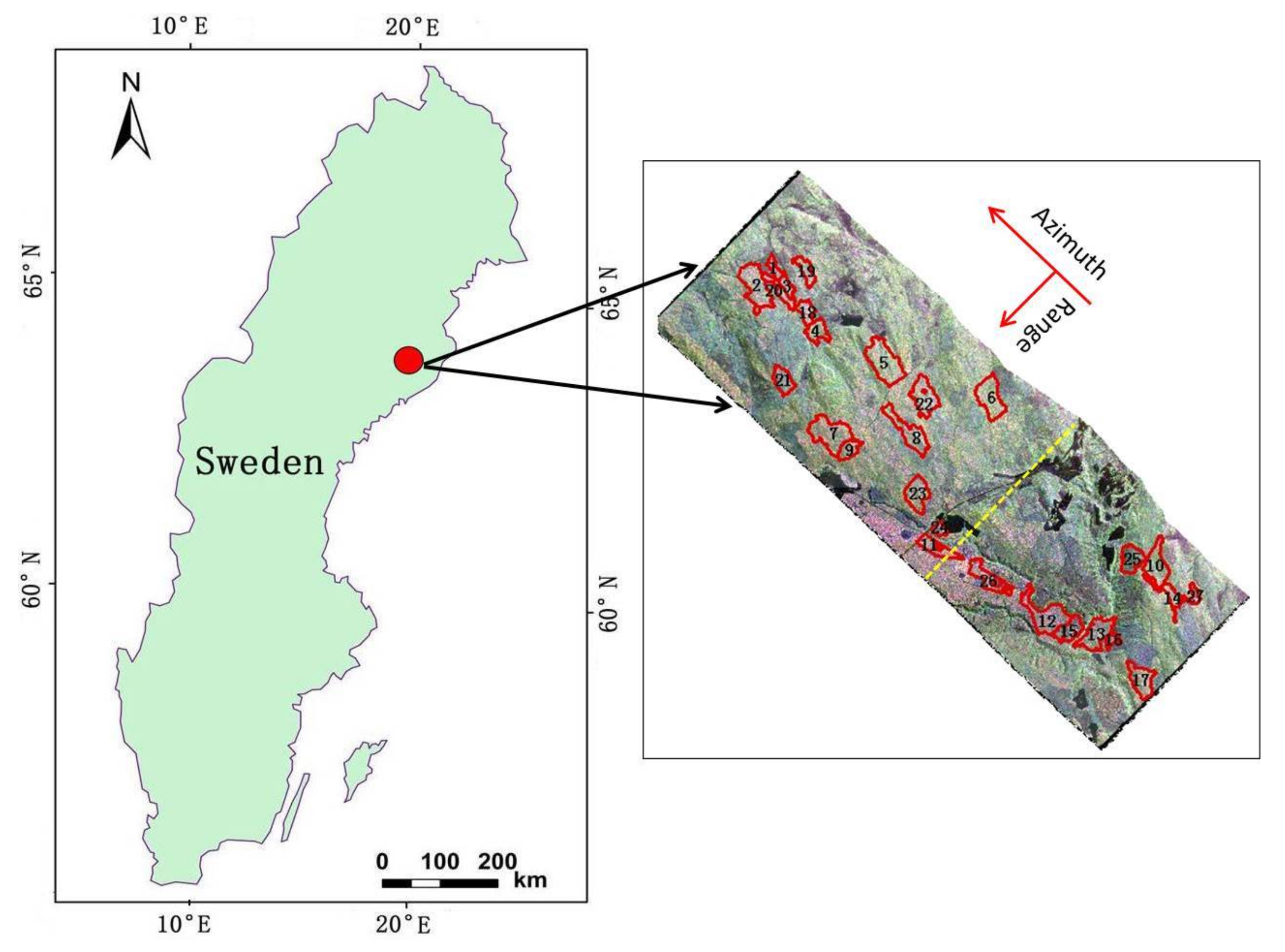
The test site is located in the Krycklan river catchment (64°16′ N, 19°46′ E) in northern Sweden (Figure 1), which is about 50 km northwest of Umea and covers approximately 9390 ha. It has become the test site for field-based forest research at the Faculty of Forest Sciences, Swedish University of Agricultural Sciences. The dominating forest type is mixed coniferous, including Norway spruce, Scots pine, and Birch [57]. In addition, there are some other small deciduous trees such as Aspen and Rowan. The dominating soil is moraine, with variations in thickness. This area is hilly, with elevation variations from 100 to 400 m throughout the whole scene, and surface slopes of up to 20° [44].
2.2. Field Data
The field survey data were collected and processed as a part of the BioSAR campaign in 2008 [58]. Twenty-seven forest stands with sizes ranging between 3.07 and 24.34 ha (boundaries are showed in Figure 1) were selected for the validation experiment. Within each stand, eight to 13 circular sample plots were laid out with a systematic spacing of 50 to 160 m, depending on the size of the area. The spacing in each stand was confirmed with the aim of obtaining 10 plots, having a radius of 10 m. The total number of plots was 310. In these plots, all trees with a diameter at breast height (DBH) greater than 4 cm were calipered and recorded. On the basis of probability proportional to their basal area, 1.5 sample trees were randomly selected from each plot to measure the height and age. Other parameters were also collected, such as the vegetation type and soil type. The biomass of different tree species, including the stem, bark, branches, and needles, but excluding the stump and roots, was calculated based on Petersson’s biomass functions [59]. In addition, the biomass of each tree species was divided into three components, namely trunks, branches, and leaves. Due to seasonal reason, the leaf biomasses of the deciduous forests were not calculated. Table 1 describes the main features of the 27 forest stands.
2.3. Polarimetric SAR Data
The P-band fully polarimetric SAR data over this study area were acquired in the framework of the European Space Agency (ESA) BioSAR 2008 campaign in the repeat-pass mode. The SAR system used in this campaign was the German Aerospace Center’s (DLR) E-SAR airborne system [58]. The platform height was about 4091 m above ground and the pixel spacing was 1.6 m and 2.12 m in the azimuth direction and slant range, respectively. Four fully polarimetric SAR images were selected for the interferometric process. There were two master images and two slave images with two different flight tracks (314° and 134° from north). In this study area, there were 12 P-band fully polarimetric SAR data in two different flight tracks. These data could constitute five pairs of PolInSAR data in each direction and their baselines were 8 m, 8 m, 16 m, 24 m, and 32 m, respectively. Kugler et al. evaluated the multifaceted effect of the effective spatial baseline by analyzing the vertical wavenumber (Kz). He concluded that a good choice to get reliable forest height estimates with sufficient accuracy for single baseline acquisitions is to select Kz ranging from 0.05 to 0.15 rad/m [60]. According to our statistics of five pairs of PolInSAR datasets in the two flight directions, we found that the baselines of 32 m in both two flight directions can better fulfill the above condition of Kz. Detailed information on these two baselines of PolInSAR datasets is listed in Table 2. The basic data processing including terrain-correction and image-registration were done by the DLR. In addition, an airborne LiDAR measurement was also conducted in the study area to serve as a reference for the parameters estimation. The LiDAR measurement as a part of the BIOSAR 2008 campaign was performed on August 2008 with the TopEye system S/N 425 mounted on a helicopter. Details of the LiDAR data can be found in [58].
3. Methodology
In order to obtain a new parameter from the tomographic profile and achieve a more accurate forest AGB estimation, we firstly acquire two scattering mechanisms by the Phase Diversity (PD) coherence optimal algorithm and calculate the forest height and ground phase. Secondly, the vertical profile of a single pixel is obtained based on the PCT technique with the volume scattering mechanism. Then, we calculate the average vertical distribution of the relative reflectance, according to the polygonal boundary of the forest stand. Thirdly, a new parameter for biomass estimation is proposed by establishing the backscatter power loss area. Finally, the estimation model of the forest AGB is constructed by combining the new parameter and other parameters from the tomographic profile described in [56]. The flowchart is shown in Figure 2.
3.1. Polarization Coherence Tomography
The vertical profile function in penetrable volume scattering is reconstructed by the single-baseline PCT technique. The main observable in PCT is the volume scattering complex interferometric coherence, which depends on vertical structure variations [53]. Therefore, this dependence relationship can be used to build 3-D imaging and extract physical parameters. The complex coherence is shown as follows [53]:
where
The complex interferometric coherence is related to the polarization state w. The vertical wavenumber kZ is related to the interferometric baseline, Z0 is the position of the bottom of the vegetation layer, hv is the vegetation height, and ϕ0 is the topographic phase. f(Z) is the vertical structure function, which physically represents the vertical variations of the scattering signal at a point in the SAR image [61]. It is bounded from the underlying surface to the top of the vegetation layer and can be developed efficiently in a Fourier-Legendre series as shown in (2):
where denotes the Legendre coefficient, and represents the Legendre polynomials with vertical variable . Then, the complex coherence for f(Z) can be rewritten as [59]:
where fi(i = 1,2,…,n) represents the Legendre polynomial parameter at order i, which is a function of the single parameter kv = kZhv/2, and ai0 is the Legendre coefficient. Equation (3) shows that the coherence can be seen as an algebraic sum of a series of structural functions.
Although multi-baseline PCT provides the potential to improve the resolution of the tomographic profile [53], it increases the number of unknown parameters, thereby increasing the computational complexity. However, single-baseline PCT only requires the second order of the Legendre series to describe the variations of the vertical profile, which is the simplest way to be implemented. In this case, obtaining the second order vertical structure function requires estimating two unknown coefficients (a10, a20) in Equation (3). We use a matrix inversion of Equation (4) to achieve this purpose.
where is the vertical structure function, which varies with the polarization state, represents the second order expansion of Fourier-Legendre polynomials, and is the vertical position from (0, hv).
Before implementing the PCT algorithm, we need to estimate the priori information of vegetation height hv and topographic phase ϕ0. We exploit the widely used random volume over ground (RVOG) model and three-stage inversion method to obtain forest height and topographic phase [41,62]. In addition, we also note that the PCT algorithm involves two polarization modes: the dominant volume scattering and the dominant ground surface scattering. Cloude [53] proposed two polarization channels, which are HV and HH-VV, representing the volume and ground surface scattering, respectively. However, the HV channel also has some ground surface scattering contributions, which leads to pure volume coherence error to vertical profile reconstruction. Therefore, we use the phase diversity (PD) coherence optimization algorithm to find the optimal polarization modes (i.e., PDhigh and PDlow) in the polarized space, thereby separating the two-phase centers maximally. The higher phase PDhigh corresponds to the “pure” volume scattering phase and the lower phase PDlow corresponds to the “pure” ground surface scattering phase [63].
3.2. The Retrieval Method of Canopy Height (Hac)
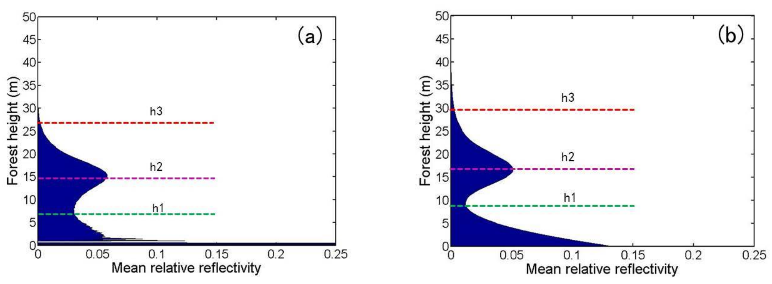
According to the PCT algorithm, the tomographic profile at the pixel scale can be obtained with a 0.2 m interval in vegetation heights [54,64]. The profile values represent relative reflectivity values. However, the relative reflectivity of a single pixel is unrelated to forest biomass, because it is randomly distributed and unable to represent the vertical structure [56]. Therefore, the average of the stand scale is used to obtain change rules of the vertical structure. As shown in Figure 3, we use stands No. 6 and No. 13 of the study area to analyze the vertical distribution of average relative reflectivity. In Figure 3, the vertical distribution curve of the average relative reflectivity is divided into upper and lower parts by h1, and the envelope between h1 and h3 is the distribution of the relative reflectivity values of forest canopy. h1 is the height of the forest corresponding to the inflection point of the upper and lower parts of the curve, and h3 represents the height of the upper half of the curve with the relative reflectivity value closest to 0.001. These data between h1 and h3 constitute the first envelope. h2 is the height position where the relative reflectivity value is the maximum in the first envelope, and the data between 0 and h2 form the second envelope.
After obtaining the vertical distribution of average relative reflectivity, the relationship between the curve and the forest biomass needs to be established. The parameters (Table 3) were obtained by parameterizing the average relative reflectivity [56]. P1 is the ratio of the peak value to the first envelope span. P2 is the integral of the relative reflectivity multiplied by the height in the first envelope. P3, P4 (TomoH), and P5 are the maximum probability, the mean, and the standard deviation of the fitted Gaussian function of the first envelope, respectively. P6 and P7 are the reciprocal of the relative reflectivity summation of the first and second envelopes, respectively. P8 represents the ratio of P6 to P7. P9 is the relative reflectivity summation between h1 and h2 multiplied by the relative reflectivity summation between h2 and h3. P10 represents the integral of the relative reflectivity multiplied by the corresponding height from 0 to h3. These parameters were defined without physical characteristics [56]. Among these parameters, P4 (the tomographic height (TomoH)) is considered as the most important parameter for forest AGB estimation. However, TomoH only corresponds to the highest volume relative reflectivity, which is lower than the actual forest height.
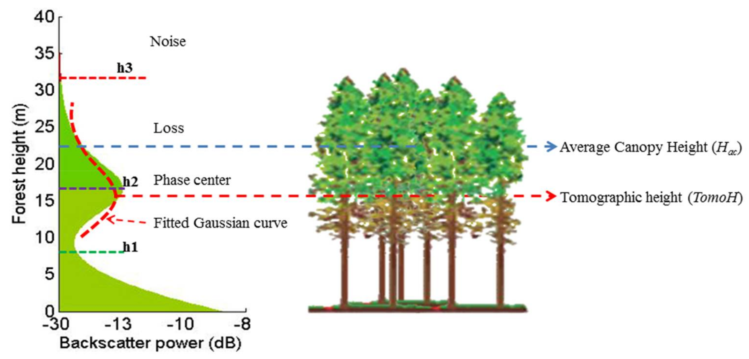
In order to find a parameter closer to the true canopy height of the stand, we characterize the average relative reflectivity as the backscattered power distribution, and then divide the average relative reflectivity distribution of the forest canopy into three parts, taking the No. 13 stand as an example (Figure 4). The first part (between h1 and h3) corresponds to the canopy phase zone, where most of the backscatter is concentrated. Its maximum value corresponds to the stand canopy phase center position, i.e., h2. The second part (between h2 and h3) is the backscatter power loss zone, where the backscatter undergoes a loss along the vertical direction from h2 to h1. The third part (above h3) is the noise zone, where the backscatter power is mostly contributed by noise, unlikely to be associated with physically relevant components. A parameter related to the average height of the stand can be extracted by analyzing the power loss value in the first envelope [50,51,52], which is:
where is the height of the average phase center of each stand, i is the stand serial number, is the backscattering power at location of stand i, and z is the value ranging from to h3. The power loss value K ranges from 0 to 1 with the step of 0.1. The optimal K is determined by the forest height that is closest to the true value obtained by LiDAR [51]. We name the corresponding forest height as the average canopy height Hac.
3.3. Model Construction and Validation
Since the power function can be used to effectively express the relationship between SAR parameters and biomass [56,65], we use a stepwise regression method to construct a multiple linear biomass estimation model with the natural logarithm of the SAR parameters.
where B is the biomass (t ha−1), and ai is the coefficient corresponding to the extracted parameters Xn from tomographic profiles.
The stepwise regression method is employed to find the best combination of independent variables to predict the dependent variable. The method introduces the independent variables to the regression model one by one (from small to large), and only those satisfying the test value F remain in the model. Usually, the remaining variables are significant and have large contributions to dependent variable estimation. When no more variables are eligible for inclusion or removal, the process is terminated. After obtaining the estimation model, we must also consider the problem of collinearity between variables. Generally, this problem can be indicated by the values of tolerance and variance inflation factor (VIF) [66].
In this paper, the three independent variables Hac, P6, and P7 are considered more sensitive to forest biomass than other parameters. The canopy height Hac is a new parameter proposed by analyzing the variation of the backscattering power of forest, and P6 and P7 are the reciprocal of the relative reflectivity summation of the first (h1–h3) and second (0–h1) envelopes, respectively. In this study, we use the m-fold (13-fold) cross-validation experiments to test the accuracy of the multiple linear biomass estimation models. We divide the forest stands into 10 groups equally, one of which is used for validation and the others are applied to regression models.
4. Experimental Results and Analysis
4.1. Tomographic Profiles
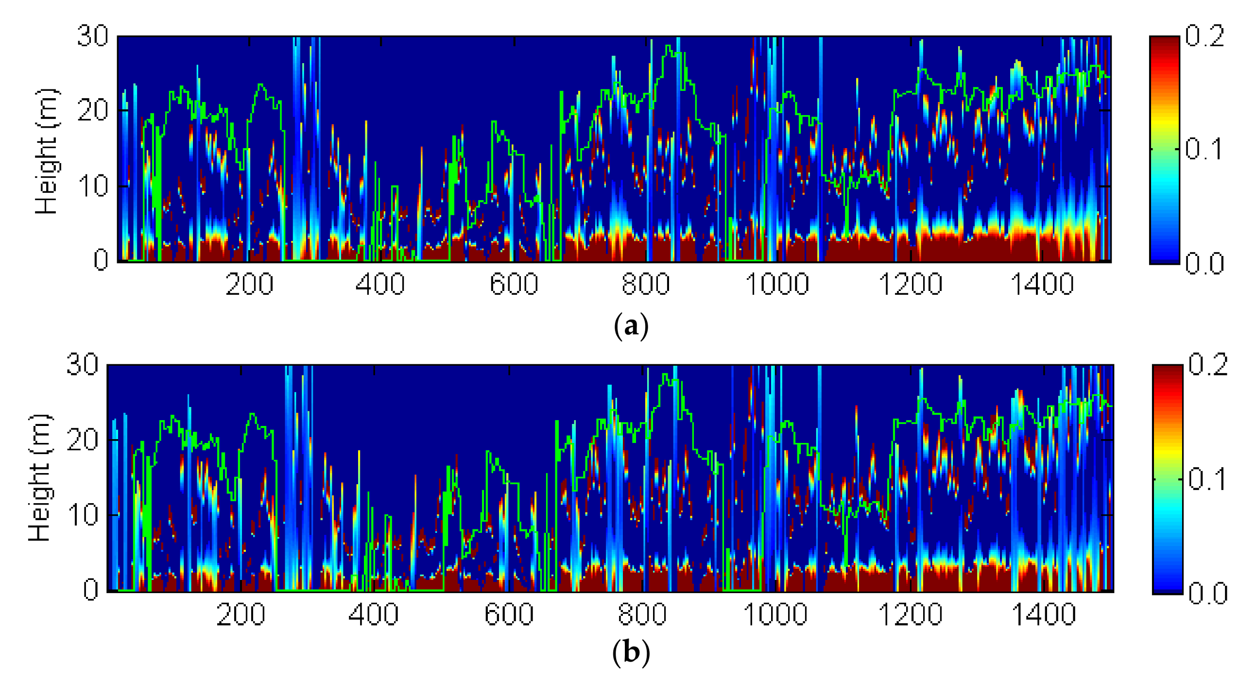
The vertical structure functions are reconstructed at PDhigh, PDlow, HV, and HH-VV polarimetric channels. The tomographic profiles in the 2500th line (yellow line in Figure 1) along the range direction are demonstrated in Figure 5, where the horizontal axis is the pixel position, the vertical axis is the forest height, and the different colors represent the intensity of relative reflectivity.
From Figure 5, it can be observed that the effect of different polarimetric channels on the tomographic profile reconstruction is significant. In the HH-VV polarimetric channel, where the surface scattering is dominant, the relative reflectivity values are mainly distributed in the ground surface layer. In the HV polarimetric channel, volume scattering is the dominant scattering mechanism and its scattering center of the interferometric phase is closer to the vegetation canopy top than that of the HH-VV channel. However, the HV channel still retains an amount of ground surface scattering contributions, which leads to pure volume coherence error affecting tomographic profile reconstruction. It means the relative reflectivity values still have a high distribution in the ground surface. From the visual perspective of Figure 5a,b, the difference of relative reflectivity vertical distribution is relatively small.
The relative reflectivity distributions are obviously different in PDlow (Figure 5c) and PDhigh (Figure 5d) channels. We note that the ground surface has high reflectivity values distribution in the PDhigh channel, which may be caused by an underlying shrub layer there. In addition, compared with the other three channels, the PDhigh channel contains more abundant vegetation information, which is conducive to extract vegetation parameters. Hence, in this paper, we use the tomographic profile of the PDhigh channel for analysis.
4.2. Parameter Retrieval
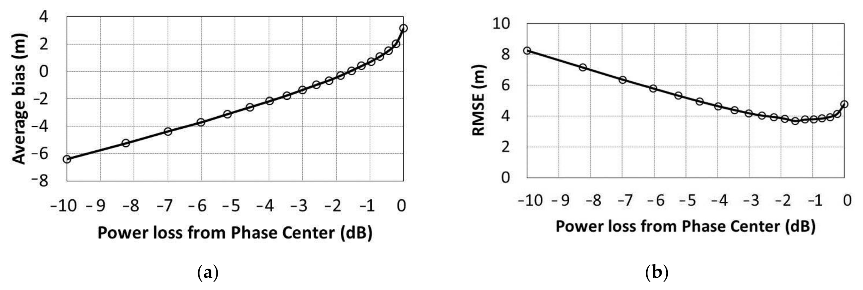
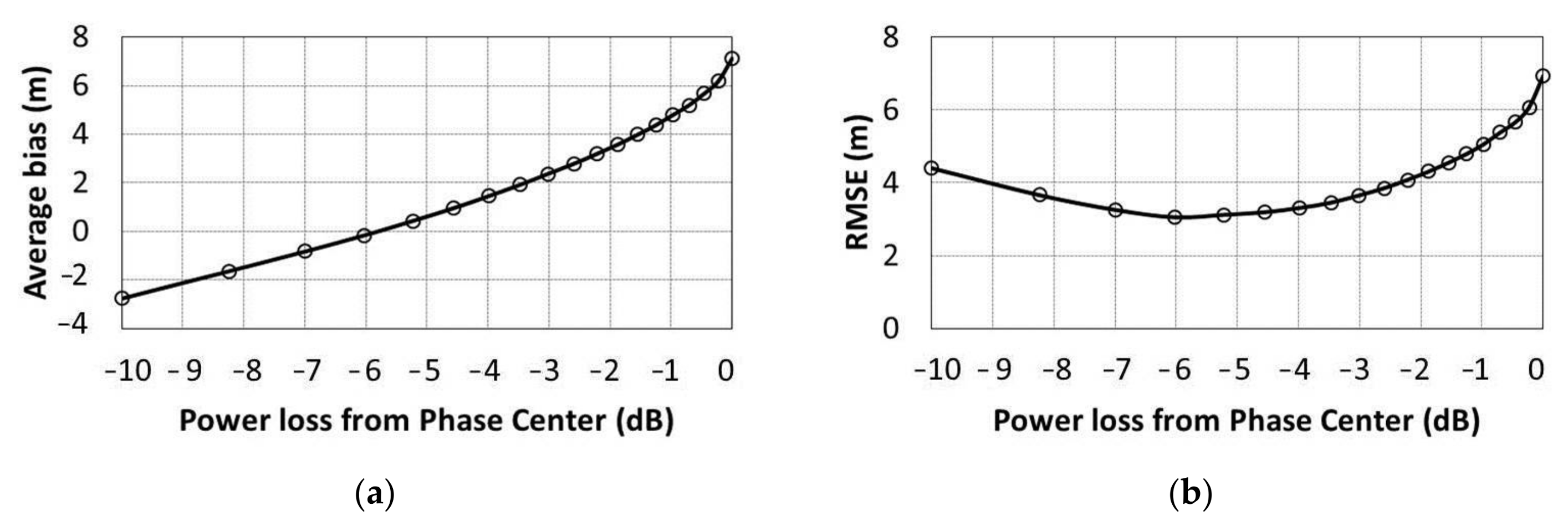
According to the method described in Section 3.2, we retrieve the new parameter of average canopy height Hac from the average tomographic profile of each stand (Figure 4). Using the top-of-canopy height LiDAR model [51], we can get the parameter’s location corresponding to a power loss value in each stand, with respect to the stand canopy phase center, ranging from −10 dB to 0 dB. Figure 6 and Figure 7 present the average bias of the stand height and the root mean square error (RMSE) with respect to the LiDAR measurements in different flight tracks, respectively. In the power loss interval of the 314 deg. flight direction, the average bias of 27 forest stands reaches the maximum at the stand canopy phase center, which is 3.162 m. The minimum value is −6.409 m, and the overall trend increases with the power loss from the phase center, which is close to 0 m at −1.549 dB. The RMSE also reaches the maximum at the stand canopy phase center, which is 8.255 m, while the minimum RMSE is found at −1.549 dB. In the power loss interval of the 134 deg. flight direction, the average bias also reaches the maximum at the stand canopy phase center, which is 7.126 m. The minimum value is −2.765 m, and the overall trend is the same as the 314 deg. flight direction increasing with the power loss from the phase center, which is close to 0 m at −6.0206 dB (Figure 7a). The RMSE also reaches the maximum at the stand canopy phase center, which is 7.862 m, while the minimum RMSE is 2.954 at −6.0206 dB (Figure 7b). These results show that −1.549 dB and −6.0206 dB are the optimal power loss values for retrieving the new parameter Hac in the two different flight directions, respectively.
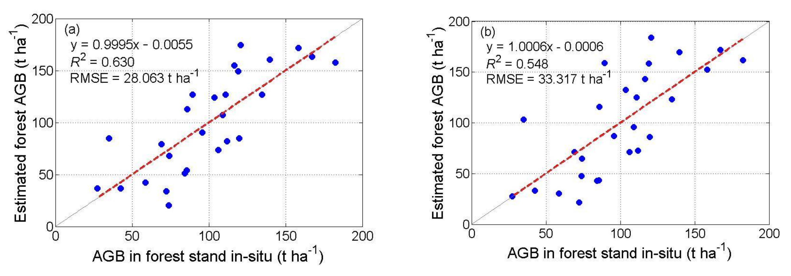
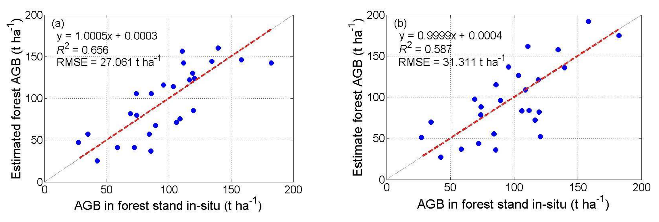
The forest heights corresponding to the power loss values of −1.549 dB and −6.0206 dB are extracted for each forest stand in different flight directions, respectively. We use TomoH [56] to evaluate the performance of parameter Hac in the estimation of AGB. In order to assess the sensitivity of the parameters Hac and TomoH to the forest biomass, respectively, the simple linear model is used to estimate the biomass of 27 forest stands. The estimated biomasses are tested with in situ AGB for each forest stand. As shown in Figure 8 and Figure 9, in the 314 deg. flight direction, the value of the correlation coefficient R2 using the parameter Hac is 0.630, which is much higher than that of TomoH (0.548). Also, the RMSEs obtained by Hac and TomoH are 28.063 t ha−1 and 33.317 t ha−1, respectively. In the 134 deg. flight direction, the RMSEs obtained by Hac and TomoH are 27.061 t ha−1 and 31.311 t ha−1, respectively. Obviously, the sensitivity and the accuracy of Hac inversion are higher than the values of the TomoH inversion in the two different flight directions, respectively, which means that Hac is more helpful for the estimation of forest biomass with P-band ESAR data in the test site.
4.3. Forest AGB Estimation
In this section, we construct a reasonable forest AGB estimation model in the test site using parameter Hac and the nine parameters (P1–P3 and P5–P10) described in [56]. Table 4 shows the results of estimation models obtained through the multiple linear stepwise regression method with the F test. Hac1 to Hac10 are the ten stepwise regression models with parameter Hac and the nine parameters (P1–P3 and P5–P10) in the 314 deg. flight direction. Based on different parameters, these models can be divided into two categories: one category includes parameters Hac and P6 (Hac1, Hac3, Hac5, Hac7, Hac9, Hac11, Hac13); and the other includes Hac, P6, and P7 (Hac2, Hac4, Hac6, Hac8, Hac10, Hac12, Hac14), which indicates that Hac, P6, and P7 are more sensitive to forest biomass than other parameters. According to these models, we can choose one of the best models for biomass estimation in the two categories, respectively. When using the same method to obtain estimation models with Li’s ten parameters (P1–P10), including TomoH, ten models are also obtained in the 314 deg. flight direction. However, based on the same rules, we only choose the best two models for comparison, namely TomoH1 and TomoH2. In addition, we also list the best models using different parameters in the 134 deg. flight direction, named Hac15, Hac16, TomoH3, and TomoH4 (Table 4).
According to Table 4, from models Hac1 to Hac14, considering only collinearity between variables cannot select the best models, because these parameters do not appear to have serious collinearity problems according to the tolerance and variance inflation factor. However, when we consider the correlation coefficient in this table, Hac3 and Hac8 will perform relatively better than other models, whose R2 values are 0.734 and 0.798, respectively. When considering the validated error, tolerance, and variance inflation factor together, we still find that Hac3 and Hac8 are more suitable for forest AGB estimation than other models in the two categories. Then, we choose these four models for analysis in the two different flight directions, respectively. Hac3, Hac8, TomoH1, and TomoH2 belong to the 314 deg. flight direction, whereas Hac15, Hac16, TomoH3, and TomoH4 belong to the 134 deg. flight direction.
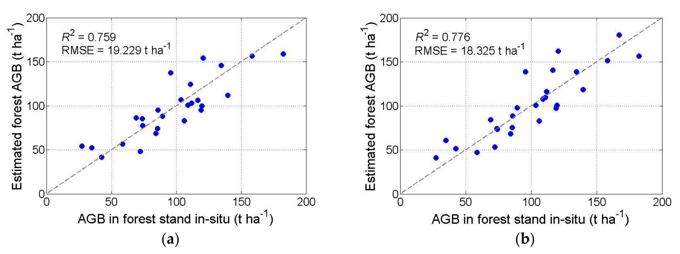
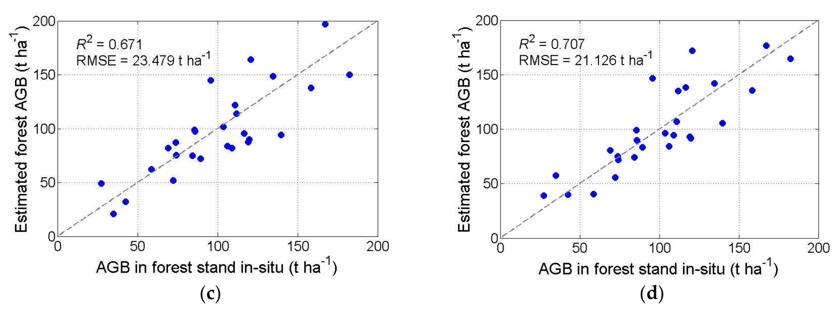
The comparison results with field data are showed in Figure 10 and Figure 11. In the 314 deg. flight direction (Figure 10), the correlation coefficient value between field data and AGB derived by Hac8 is 0.761, which is higher than the values obtained by Hac3, TomoH1, and TomoH2 (0.728, 0.573, and 0.687, respectively). Additionally, the RMSEs of Hac3 and Hac8 are 19.941 t ha−1 and 18.824 t ha−1, respectively, which are lower than those of TomoH1 (24.834 t ha−1) and TomoH2 (21.219 t ha−1). Obviously, the performance of Hac8-based inversion is better than that of other models. In the 134 deg. Flight direction (Figure 11), the performance of Hac16-based inversion is better than that of other models, whose correlation coefficient value is 0.776 and RMSE is 18.325 t ha−1.
5. Discussion
Traditional studies on the PCT technology usually focus on forest vertical profile generation [59,61], with rare consideration of the relationship between the vertical profile and the forest parameters. In this study, all the parameters for AGB inversion were extracted by analyzing the geometric characteristics of the average vertical profiles within the forest stand [55,56]. These parameters are mathematically defined without considering physical scattering mechanisms of forest. In references [55,56], TomoH (i.e., P4) is the most important parameter for the estimation of forest AGB. Nevertheless, TomoH only corresponds to the highest volume relative reflectivity, which is lower than the actual forest height, especially for long wavelengths (such as P-band) SAR data [55]. In this study, we use the PCT technique and P-band airborne PolInSAR data to generate the average vertical profile. A new parameter (i.e., Hac) for estimating forest AGB is retrieved through analyzing the variation of the vertical backscatter power, which considers the physical scattering attenuation when radar echo penetrates into the forest. The experiment results (Figure 8 and Figure 9) show that better accuracies are achieved for AGB inversion, which demonstrates that Hac performs relatively better than TomoH. Additionally, we combine Hac with Li’s nine parameters to construct the forest AGB estimation model by a multiple linear stepwise regression method. The results in Table 4, as well as Figure 10 and Figure 11, show that the combination has a better performance than only using Li’s ten parameters, which also indirectly verify the validity and reliability of the new parameter in estimating forest AGB.
Forest biomass estimation is a timely topic, and many scholars have used different data and methods to estimate biomass in different regions. In the test site of this paper (krycklan area), Ulander et al. [67] used a multiple linear regression model based on P-band multi-polarization backscatter to estimate biomass, and the RMSE varied in the range 29–42 t ha−1. Neumann et al. [44] used parametric (linear regression) and non-parametric (random forest, support vector machine) methods to assess biomass estimation performance with polarimetric interferometric synthetic aperture radar (PolInSAR) data at L- and P-band in this test area, and the cross-validated biomass RMSE was reduced to 23 t ha−1 in the best case at P-band. Compared with these methods, PCT technology can extract forest vertical structures from the vertical distribution of relative reflectivity and has the potential to improve biomass estimation. In addition, the potential of P-band TomoSAR to characterize forest structure was assessed in a number of studies relating forest vertical structure to forest biomass [50,51,52]. Compared with TomoSAR technology, the single baseline PCT reduces the amount of data, but it has the problem of inverting the instability of the vertical profile of relative reflectivity in some places (Figure 5) and multi-baseline PCT technology may improve the phenomenon. Moreover, we note that the optimal power loss value for forest parameter extraction in this test site is different at two different flight tracks, and the value also should be different for other test sites, since power loss is always related to the vertical resolution, forest types, density, etc. [58].
6. Conclusions
In this paper, we propose a method based on the polarimetric coherence tomography for forest AGB inversion. A new parameter of average canopy height (Hac) considering scattering attenuation is introduced for AGB inversion. Two pairs of P-band E-SAR full polarimetric SAR data covering the Krycklan river catchment in northern Sweden are selected for experiments. The results show that the tomographic profiles are greatly influenced by the polarimetric channels, and the PD algorithm can provide two more suitable polarimetric channels for the PCT technology. Referenced to the LiDAR forest height, in the 314 deg. flight direction, the power loss of −1.549 dB relative to the canopy phase center’s power is confirmed to be the optimal value and is used to retrieve the new parameter of average canopy height Hac with average bias and RMSE. In contrast with the tomographic height (TomoH), the new parameter Hac is shown to be closer to the top of the stands, and has more advantages for forest AGB inversion. Following this, a high performance and precision inversion model is constructed by combining parameter Hac with other parameters (Li’s parameters). The RMSE is 18.824 t ha−1 in the test area. The same conclusion is reached with the data we use in the other flight direction. The RMSE is 18.325 t ha−1. In this study, we try to introduce a parameter considering scattering characteristics, rather than just from geometric characteristics, for improving the accuracy of forest AGB inversion.
Acknowledgments
The work was supported by the National Natural Science Foundation of China (No. 41531068, 41671356 and 41371335), the Natural Science Foundation of Hunan Province, China (No. 2016JJ2141), and Innovation Foundation for Postgraduate of Central South University, China (No. 2017zzts179). Additionally, the experimental datasets are supported by PA-SB ESA EO Project Campaign (ID. 14655, 14751).
Author Contributions
Haibo Zhang conceived the idea, performed the experiments, and wrote and revised the paper; Changcheng Wang contributed some ideas, analyzed the experimental results, and revised the paper; Jianjun Zhu supervised the work and contributed some ideas; Haiqiang Fu, Qinghua Xie, and Peng Shen contributed to the discussion of the results.
Conflicts of Interest
The authors declare no conflict of interest.
References
- Bonan, G.B. Forests and climate change: Forcings, Feedbacks, and the Climate Benefits of Forests. Science 2008, 320, 1444–1449. [Google Scholar] [CrossRef] [PubMed]
- Kindermann, G.E.; McCallum, I.; Fritz, S.; Obersteiner, M. A global forest growing stock, biomass and carbon map based on FAO statistics. Silva Fenn. 2008, 42, 387–396. [Google Scholar] [CrossRef]
- Pan, Y.; Birdsey, R.A.; Houghton, R.; Kauppi, P.E.; Kurz, W.A.; Phillips, O.L.; Shvidenko, A.; Lewis, S.L.; Canadell, J.G.; Ciais, P.; et al. A Large and Persistent Carbon Sink in the World’s Forests. Science 2011, 333, 988–993. [Google Scholar] [CrossRef] [PubMed]
- Askne, J.I.H.; Fransson, J.E.S.; Santoro, M.; Soja, M.J.; Ulander, L.M.H. Model-based biomass estimation of a Hemi-Boreal forest from multitemporal TanDEM-X acquisitions. Remote Sens. 2013, 5, 5725–5756. [Google Scholar] [CrossRef]
- Houghton, R.A. Aboveground forest biomass and the global carbon balance. Glob. Chang. Biol. 2005, 11, 945–958. [Google Scholar] [CrossRef]
- Houghton, R.A.; Hall, F.; Goetz, S.J. Importance of biomass in the global carbon cycle. J. Geophys. Res. Biogeosci. 2009, 114. [Google Scholar] [CrossRef]
- Lu, D. The potential and challenge of remote sensing-based biomass estimation. Int. J. Remote Sens. 2006, 27, 1297–1328. [Google Scholar] [CrossRef]
- Powell, S.L.; Cohen, W.B.; Healey, S.P.; Kennedy, R.E.; Moisen, G.G.; Pierce, K.B.; Ohmann, J.L. Quantification of live aboveground forest biomass dynamics with Landsat time-series and field inventory data: A comparison of empirical modeling approaches. Remote Sens. Environ. 2010, 114, 1053–1068. [Google Scholar] [CrossRef]
- Gibbs, H.K.; Brown, S.; Niles, J.O.; Foley, J.A. Monitoring and estimating tropical forest carbon stocks: Making REDD a reality. Environ. Res. Lett. 2007, 2, 045023. [Google Scholar] [CrossRef]
- Uddin, K.; Gilani, H.; Murthy, M.S.R.; Kotru, R.; Qamer, F.M. Forest Condition monitoring using very-high-resolution satellite imagery in a remote mountain watershed in Nepal. Mt. Res. Dev. 2015, 35, 264–277. [Google Scholar] [CrossRef]
- Yu, Y.; Saatchi, S. Sensitivity of L-band SAR backscatter to aboveground biomass of global forests. Remote Sens. 2016, 8, 522. [Google Scholar] [CrossRef]
- Anderson, G.L.; Hanson, J.D.; Haas, R.H. Evaluating Landsat thematic mapper derived vegetation indices for estimating above-ground biomass on semiarid rangelands. Remote Sens. Environ. 1993, 45, 165–175. [Google Scholar] [CrossRef]
- Steininger, M.K. Satellite estimation of Tropical Sencondary forest above-ground biomass: Data from Brazil and Bolivia. Int. J. Remote Sens. 2000, 21, 1139–1157. [Google Scholar] [CrossRef]
- Baccini, A.; Laporte, N.; Goetz, S.J.; Sun, M.; Dong, H. A first map of tropical Africa’s above-ground biomass derived from satellite imagery. Environ. Res. Lett. 2008, 3, 45011–45019. [Google Scholar] [CrossRef]
- Sinha, S.; Jeganathan, C.; Sharma, L.K.; Nathawat, M.S. A review of radar remote sensing for biomass estimation. Int. J. Environ. Sci. Technol. 2015, 12, 1779–1792. [Google Scholar] [CrossRef]
- Su, Y.J.; Guo, Q.H.; Xue, B.L.; Hu, T.Y.; Alvarez, O.; Tao, S.L.; Fang, J.Y. Spatial distribution of forest aboveground biomass in China: Estimation through combination of spaceborne lidar, optical imagery, and forest inventory data. Remote Sens. Environ. 2016, 173, 197–199. [Google Scholar] [CrossRef]
- Funning, G.J.; Parsons, B.; Wright, T.J. Fault slip in the 1997 Manyi, Tibet earthquake from linear elastic modelling of InSAR displacements. Geophys. J. Int. 2007, 169, 988–1008. [Google Scholar] [CrossRef]
- Furuya, M.; Satyabala, S.P. Slow earthquake in Afghanistan detected by InSAR. Geophys. Res. Lett. 2008, 35, 160–162. [Google Scholar] [CrossRef]
- Schulz, W.H.; Kean, J.W.; Wang, G. Landslide movement in southwest Colorado triggered by atmospheric tides. Nat. Geosci. 2009, 2, 863–866. [Google Scholar] [CrossRef]
- Cai, J.; Wang, C.; Mao, X.; Wang, Q. An adaptive offset tracking method with SAR images for landslide displacement monitoring. Remote Sens. 2017, 9, 830–845. [Google Scholar] [CrossRef]
- Dowdeswell, J.A.; Unwin, B.; Nuttall, A.; Wingham, D.J. Velocity structure, flow instability and mass flux on a large Arctic ice cap from satellite radar interferometry. Earth Planet. Sci. Lett. 1999, 167, 131–140. [Google Scholar] [CrossRef]
- Goldstein, R.M.; Engelhardt, H.; Kamb, B.; Frolich, R.M. Satellite radar interferometry for monitoring ice sheet motion: Application to an antarctic ice stream. Science 1993, 262, 1525–1530. [Google Scholar] [CrossRef] [PubMed]
- Lopez-Sanchez, J.M.; Vicente-Guijalba, F.; Erten, E.; Campos-Taberner, M.; Garcia-Haro, F.J. Retrieval of vegetation height in rice fields using polarimetric sar interferometry with tandem-x data. Remote Sens. Environ. 2017, 192, 30–44. [Google Scholar] [CrossRef]
- Le Toan, T.; Beaudoin, A.; Riom, J.; Guyon, D. Relating forest biomass to SAR data. IEEE Trans. Geosci. Remote Sens. 1992, 30, 403–411. [Google Scholar] [CrossRef]
- Le Toan, T.; Quegan, S.; Woodward, I.; Lomas, M.; Delbart, N.; Picard, G. Relating radar remote sensing of biomass to modelling of forest carbon budgets. Clim. Chang. 2004, 67, 379–402. [Google Scholar] [CrossRef]
- Mermoz, S.; Réjou-Méchain, M.; Villard, L.; Le Toan, T.; Rossi, V.; Gourlet-Fleury, S. Decrease of L-band SAR backscatter with biomass of dense forests. Remote Sens. Environ. 2015, 159, 307–317. [Google Scholar] [CrossRef]
- Santos, J.; Lacruz, M.; Araujo, L.; Keil, M. Savanna and tropical rainforest biomass estimation and spatialization using JERS-1 data. Int. J. Remote Sens. 2002, 23, 1217–1229. [Google Scholar] [CrossRef]
- Saatchi, S.; Marlier, M.; Chazdon, R.; Clark, D.; Russell, A. Impact of spatial variability of tropical forest structure on radar estimation of aboveground biomass. Remote Sens. Environ. 2011, 115, 2836–2849. [Google Scholar] [CrossRef]
- Carreiras, J.; Melo, J.B.; Vasconcelos, M.J. Estimating the above-ground biomass in Miombo Savanna woodlands (Mozambique, East Africa) using L-band synthetic aperture radar data. Remote Sens. 2013, 5, 1524–1548. [Google Scholar] [CrossRef]
- Mermoz, S.; Le Toan, T.; Villard, L.; Réjou-Méchain, M.; Seifert-Granzin, J. Biomass assessment in the Cameroon savanna using ALOS PALSAR data. Remote Sens. Environ. 2014, 155, 109–119. [Google Scholar] [CrossRef]
- Sandberg, G.; Ulander, L.M.H.; Fransson, J.E.S.; Holmgren, J.; Le Toan, T. L- and P-band backscatter intensity of biomass retrieval in hemiboreal forest. Remote Sens. Environ. 2011, 115, 2874–2886. [Google Scholar] [CrossRef]
- Ranson, K.J.; Sun, G. Mapping biomass of a northern forest using multi-frequency SAR data. IEEE Trans. Geosci. Remote Sens. 1994, 32, 388–396. [Google Scholar] [CrossRef]
- Saatchi, S.; Halligan, K.; Despain, D.G.; Crabtree, R.L. Estimation of forest fuel load from radar remote sensing. IEEE Trans. Geosci. Remote Sens. 2007, 45, 1726–1740. [Google Scholar] [CrossRef]
- Robinson, C.; Saatchi, S.; Neumann, M.; Gillespie, T. Impacts of spatial variability on aboveground biomass estimation from L-band radar in a temperate forest. Remote Sens. 2013, 5, 1001–1023. [Google Scholar] [CrossRef]
- Ranson, K.J.; Sun, G. Effects of environmental conditions on boreal forest classification and biomass estimates with SAR. IEEE Trans. Geosci. Remote Sens. 2000, 38, 1242–1252. [Google Scholar] [CrossRef]
- Santos, J.R.; Freitas, C.C.; Araujo, L.S.; Dutra, L.V.; Mura, J.C.; Gama, F.F.; Soler, L.S.; SantAnna, S.J.S. Airborne P-band SAR applied to the aboveground biomass studies in the Brazilian tropical rainforest. Remote Sens. Environ. 2003, 87, 482–493. [Google Scholar] [CrossRef]
- Cartus, O.; Santoro, M.; Kellndorfer, J. Mapping forest aboveground biomass in the Northeastern United States with ALOS PALSAR dual-polarization L-band. Remote Sens. Environ. 2012, 124, 466–478. [Google Scholar] [CrossRef]
- Pulliainen, J.T.; Kurvonen, L.; Hallikainen, M.T. Multitemporal behavior of L- and C-band SAR observations of boreal forests. IEEE Trans. Geosci. Remote Sens. 1999, 37, 927–937. [Google Scholar] [CrossRef]
- Fu, H.; Wang, C.; Zhu, J.; Xie, Q.; Zhao, R. Inversion of vegetation height from PolInSAR using complex least squares adjustment method. Sci. China Earth Sci. 2015, 58, 1018–1031. [Google Scholar] [CrossRef]
- Wang, C.; Wang, L.; Fu, H.; Xie, Q.; Zhu, J. The impact of forest density on forest height inversion modeling from Polarimetric InSAR data. Remote Sens. 2016, 8, 291. [Google Scholar] [CrossRef]
- Fu, H.; Wang, C.; Zhu, J.; Xie, Q.; Zhang, B. Estimation of pine forest height and underlying dem using multi-baseline P-band PolInSAR data. Remote Sens. 2017, 9, 363. [Google Scholar] [CrossRef]
- Xie, Q.; Zhu, J.; Wang, C.; Fu, H.; Lopez-Sanchez, J.M.; Ballester-Berman, J.D. A modified Dual-Baseline PolInSAR method for forest height estimation. Remote Sens. 2017, 9, 819. [Google Scholar] [CrossRef]
- Le Toan, T.; Quegan, S.; Davidson, M.; Balzter, H.; Paillou, P.; Papathanassiou, K.; Plummer, S.; Rocca, F.; Saatchi, S.; Shugart, H.; et al. The BIOMASS mission: Mapping global forest biomass to better understand the terrestrial carbon cycle. Remote Sens. Environ. 2011, 115, 2850–2860. [Google Scholar] [CrossRef]
- Neumann, M.; Saatchi, S.S. Assessing performance of L- and P-band polarimetric interferometric SAR data in estimating boreal forest above-ground biomass. IEEE Trans. Geosci. Remote Sens. 2012, 50, 714–726. [Google Scholar] [CrossRef]
- Hansen, E.H.; Gobakken, T.; Solberg, S.; Kangas, A.; Ene, L.; Mauya, E.; Næssse, E. Relative efficiency of ALS and InSAR for biomass estimation in a Tanzanian Rainforest. Remote Sens. 2015, 7, 9865–9885. [Google Scholar] [CrossRef] [Green Version]
- Pardini, M.; Kugler, F.; Lee, S.K.; Sauer, S.; Torano-Caicoya, A.; Papathanassiou, K. Biomass estimation from forest vertical structure: Potentials and Challenges for multi-baselin Pol-InSAR techniques. In Proceedings of the European Conference on PolInSAR, Rome, Italy, 24–28 January 2011; ESA: Paris, France, 2011. [Google Scholar]
- Treuhaft, R.N.; Chapman, B.D.; Dos Santos, J.R.; Goncalves, F.G.; Dutra, L.V.; Graca, P.; Drake, J.B. Vegetation profiles in Tropical forests from multibaseline lnterferometric synthetic aperture radar, field and lidar measurements. J. Geophys. Res. 2009, 114, D23110. [Google Scholar] [CrossRef]
- Treuhaft, R.N.; Goncalves, F.G.; Drake, J.B.; Chapman, B.D.; Dos Santos, J.R.; Dutra, L.V.; Graca, P.M.L.A.; Purcell, G.H. Biomass estimation in a Tropical Wet forest using Fourier transforms of profiles from lidar or interferometric SAR. Geophys. Res. Lett. 2010, 37, L23403. [Google Scholar] [CrossRef]
- Tebaldini, S. Algebraic synthesis of forest scenarios from multibaseline PolInSAR data. IEEE Trans. Geosci. Remote Sens. 2009, 47, 4132–4144. [Google Scholar] [CrossRef]
- Tebaldini, S.; Rocca, F. Multibaseline polarimetric SAR tomography of a Boreal forest at P- and L-bands. IEEE Trans. Geosci. Remote Sens. 2012, 50, 232–246. [Google Scholar] [CrossRef]
- Minh, D.H.T.; Tebaldini, S.; Rocca, F.; Le Toan, T.; Villard, L.; Dubois-Femandez, P.C. Capabilities of BIOMASS Tomography for Investigating Tropical Forests. IEEE Trans. Geosci. Remote Sens. 2015, 53, 965–975. [Google Scholar] [CrossRef]
- Minh, D.H.T.; Le Toan, T.; Rocca, F.; Tebaldini, S.; Villard, L.; Réjou-Méchain, M.; Phillips, O.L.; Feldpausch, T.R.; Dubois-Fernandez, P.; Scipal, K.; et al. SAR tomography for the retrieval of forest biomass and height: Cross-validation at two tropical forest sites in French Guiana. Remote Sens. Environ. 2016, 175, 138–147. [Google Scholar] [CrossRef] [Green Version]
- Cloude, S.R. Polarization coherence tomography. Radio Sci. 2006, 41, RS4017. [Google Scholar] [CrossRef]
- Cloude, S.R. Polarisation: Applications in Remote Sensing; Oxford University Press: New York, NY, USA, 2010. [Google Scholar]
- Luo, H.M.; Chen, E.X.; Li, Z.Y.; Cao, C. Forest above ground biomass estimation methodology based on polarization coherence tomography. J. Remote Sens. 2011, 15, 1138–1155. [Google Scholar] [CrossRef]
- Li, W.M.; Chen, E.X.; Li, Z.Y.; Ke, Y.H.; Zhan, W.F. Forest aboveground biomass estimation using polarization coherence tomography and PolSAR segmentation. Int. J. Remote Sens. 2015, 36, 530–550. [Google Scholar] [CrossRef]
- Askne, J.I.H.; Soja, M.J.; Ulander, L.M.H. Biomass estimation in a boreal forest from TanDEM-X data, lidar DTM, and the interferometric water cloud model. Remote Sens. Environ. 2017, 196, 266–278. [Google Scholar] [CrossRef]
- DLR Microwaves and Radar Institute; Swedish Defense Research Agency; Politecnico di Milano POLIMI. BIOSAR 2008: Data Acquisition and Processing Report. 2008. Available online: https://earth.esa.int/c/document_library/get_file?folderId=21020&name=DLFE-903.pdf (accessed on 17 February 2017).
- Petersson, H. Biomassafunktioner för Trädfraktioner av Tall, Gran och Björk i Sverige (in Swedish with English Summary); Swedish University of Agrivlutural Sciences: Umeå, Sweden, 1999. [Google Scholar]
- Kugler, F.; Lee, S.K.; Hajnsek, I. Forest height estimation by means of Pol-InSAR data inversion: The role of the vertical wavenumber. IEEE Trans. Geosci. Remote Sens. 2015, 53, 5294–5311. [Google Scholar] [CrossRef]
- Luo, H.M.; Li, X.W.; Chen, E.X.; Cheng, J.; Cao, C.X. Analysis of forest backscattering characteristics based on polarization coherence tomography. Sci. China Technol. Sci. 2010, 53, 166–175. [Google Scholar] [CrossRef]
- Cloude, S.R.; Papathanassiou, K.P. Three-stage inversion process for polarimetric SAR interferometry. IEEE Proc. Radar Sonar Navig. 2003, 150, 125–134. [Google Scholar] [CrossRef]
- Tabb, M.; Orrey, J.; Flynn, T.; Carande, R. Phase diversity: A decomposition for vegetation parameter estimation using polarimetric SAR interferometry. In Proceedings of the 4th European Synthetic Aperture Radar Conference (EUSAR), Cologne, Germany, 4–6 June 2002; pp. 721–724. [Google Scholar]
- Albinet, C.; Borderies, P.; Hamadi, A.; Dubois-Fernandez, P.; Koleck, T.; Angelliaume, S. High-resolution vertical polarimetric imaging of pine forests. Radio Sci. 2014, 49, 231–241. [Google Scholar] [CrossRef]
- Luckman, A.; Baker, J.; Honzák, M.; Lucas, R. Tropical forest biomass density estimation using JERS-1 SAR: Seasonal variation, confidence limits, and application to image mosaics. Remote Sens. Environ. 1998, 63, 126–139. [Google Scholar] [CrossRef]
- O’Brien, R.M. A caution regarding rules of thumb for variance inflation factors. Qual. Quant. 2007, 41, 673–690. [Google Scholar] [CrossRef]
- Ulander, L.M.H.; Sandberg, G.; Soja, M.J. Biomass retrieval algorithm based on P-band biosar experiments of boreal forest. Presented at the IGARSS, Vancouver, BC, Canada, 24–29 July 2011. [Google Scholar]
Figure 1.
The test site: P-band synthetic aperture radar (SAR) image in the Pauli basis. The red polygons indicate the forest stands.
Figure 1.
The test site: P-band synthetic aperture radar (SAR) image in the Pauli basis. The red polygons indicate the forest stands.

Figure 2.
Flowchart of forest AGB estimation. AGB: above ground biomass; PCT: polarization coherence tomography; PolInSAR: Polarimetric SAR interferometry; P1–P10: parameters.
Figure 2.
Flowchart of forest AGB estimation. AGB: above ground biomass; PCT: polarization coherence tomography; PolInSAR: Polarimetric SAR interferometry; P1–P10: parameters.
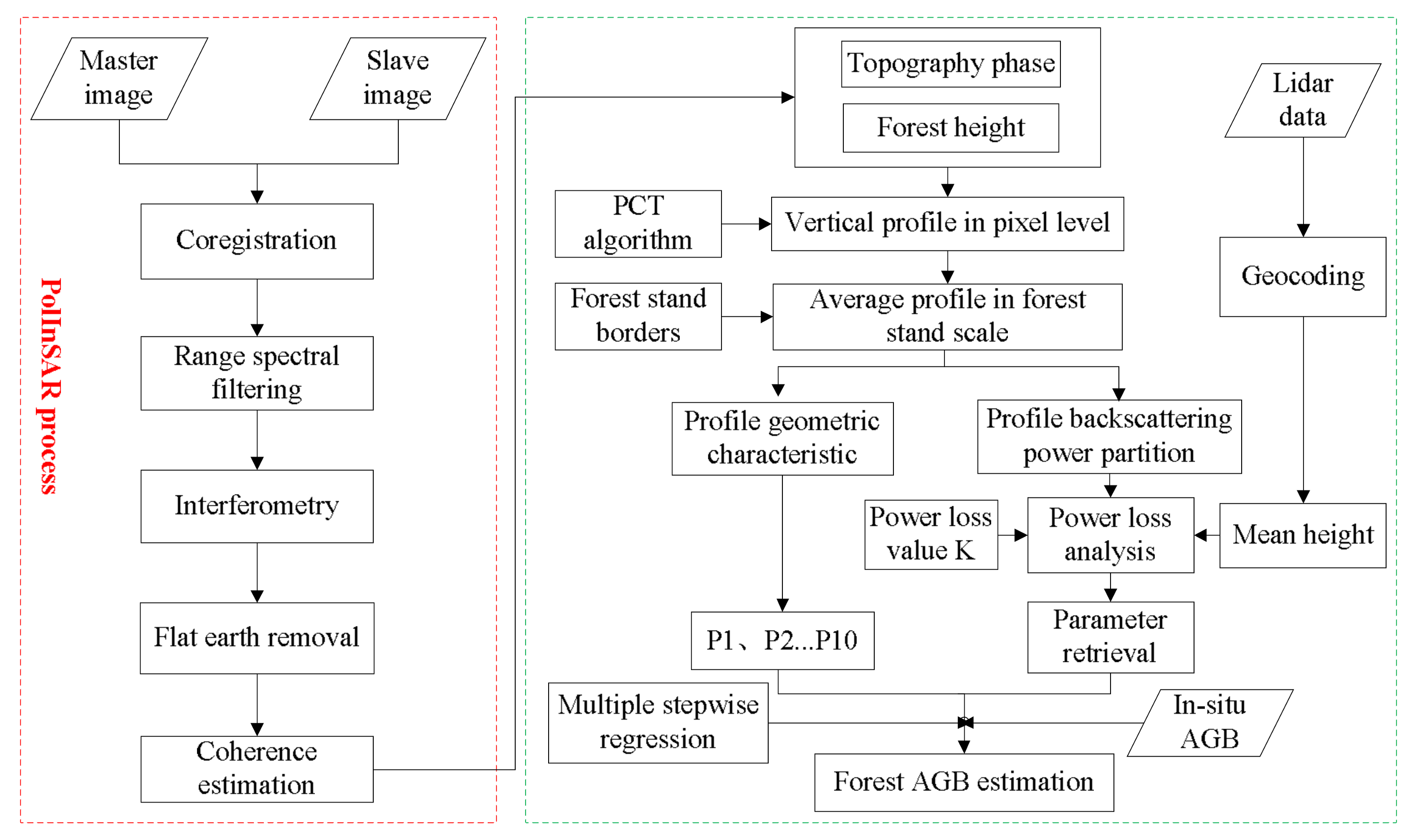
Figure 3.
Tomographic profiles of (a) stand No. 6 and (b) stand No. 13.

Figure 4.
The schematic view of the stand vertical backscatter distribution.

Figure 5.
Tomographic profiles for different polarimetric channels along the range direction in the line 2500, see the yellow dashed line in Figure 1. (a) HH-VV channel; (b) HV channel; (c) PDlow channel; (d) PDhigh channel. The green lines denote the LiDAR height. PD: phase diversity.
Figure 5.
Tomographic profiles for different polarimetric channels along the range direction in the line 2500, see the yellow dashed line in Figure 1. (a) HH-VV channel; (b) HV channel; (c) PDlow channel; (d) PDhigh channel. The green lines denote the LiDAR height. PD: phase diversity.

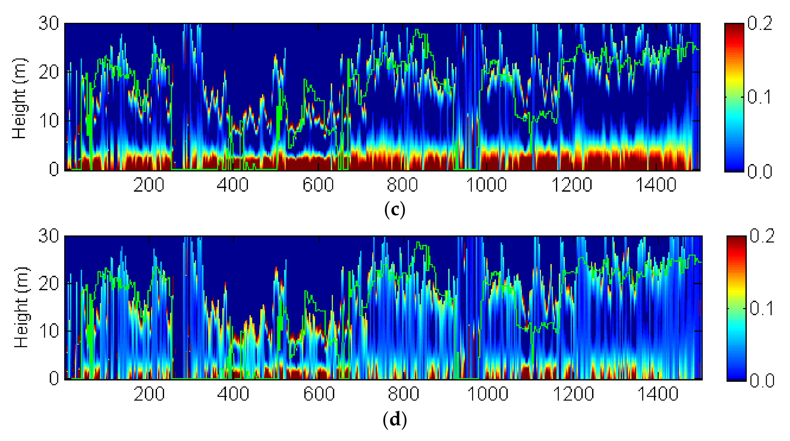
Figure 6.
Average bias and root mean square error (RMSE) in 314 deg. flight direction (a) Stand height average bias and (b) RMSE versus power loss with respect to stand average canopy phase center elevation.
Figure 6.
Average bias and root mean square error (RMSE) in 314 deg. flight direction (a) Stand height average bias and (b) RMSE versus power loss with respect to stand average canopy phase center elevation.

Figure 7.
Average bias and RMSE in 134 deg. flight direction (a) Stand height average bias and (b) RMSE versus power loss with respect to stand average canopy phase center elevation.
Figure 7.
Average bias and RMSE in 134 deg. flight direction (a) Stand height average bias and (b) RMSE versus power loss with respect to stand average canopy phase center elevation.

Figure 8.
Forest AGB estimation results using (a) Hac and (b) TomoH in 314 deg. flight direction.

Figure 9.
Forest AGB estimation results using (a) Hac and (b) TomoH in 134 deg. flight direction.

Figure 10.
Comparison between in-situ AGB and estimated forest AGB derived from model in 314 deg. flight direction (a) Hac3, (b) Hac8, (c) TomoH1, and (d) TomoH2.
Figure 10.
Comparison between in-situ AGB and estimated forest AGB derived from model in 314 deg. flight direction (a) Hac3, (b) Hac8, (c) TomoH1, and (d) TomoH2.
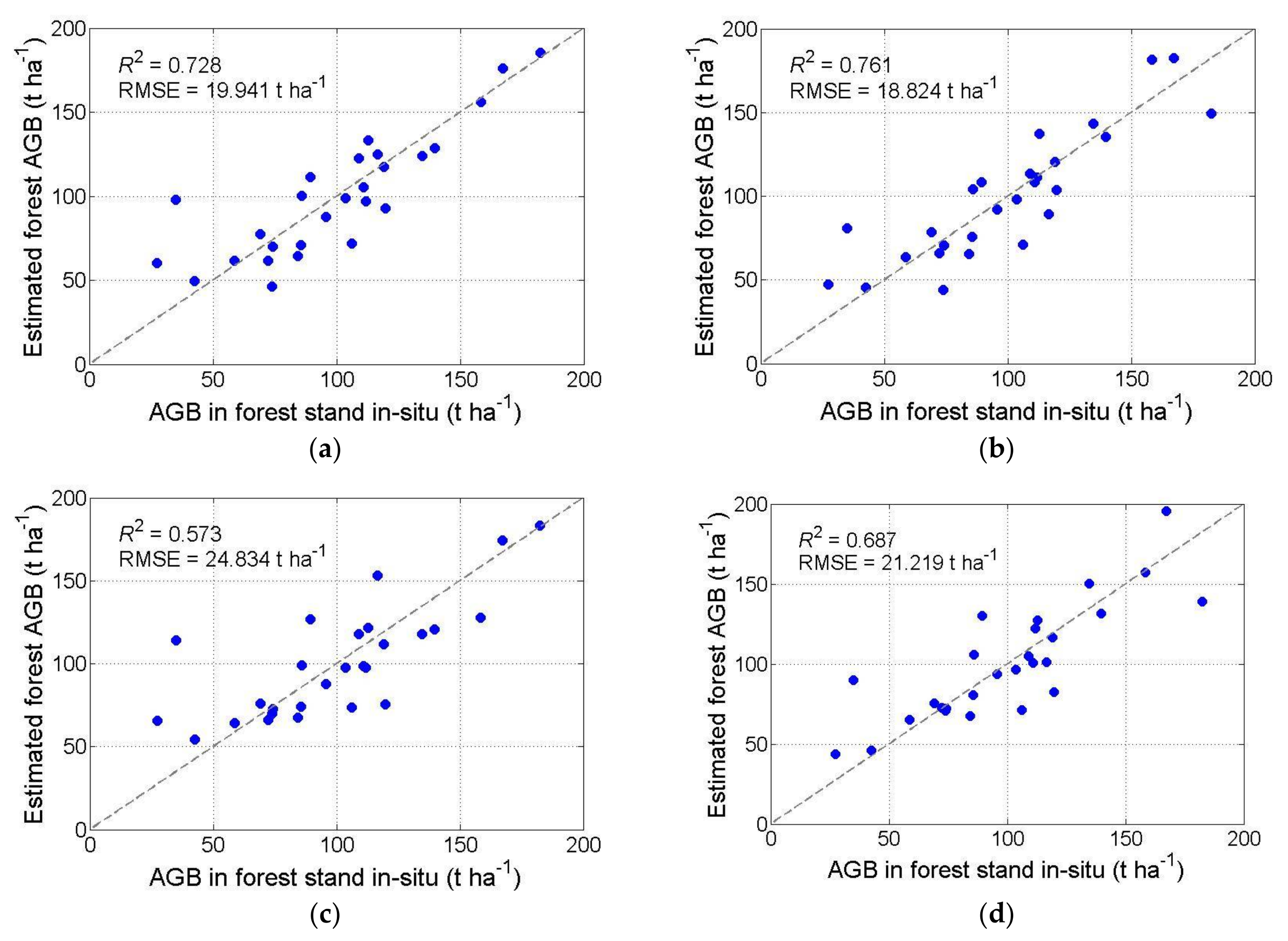
Figure 11.
Comparison between in-situ AGB and estimated forest AGB derived from model in 134 deg. flight direction (a) Hac15, (b) Hac16, (c) TomoH3, and (d) TomoH4.
Figure 11.
Comparison between in-situ AGB and estimated forest AGB derived from model in 134 deg. flight direction (a) Hac15, (b) Hac16, (c) TomoH3, and (d) TomoH4.


Table 1.
Main features of the in-situ data.
| ID | Mean DBH (cm) | Mean Height (m) | Mean Age (Year) | Biomass (t ha−1) |
|---|---|---|---|---|
| 1 | 17.6 | 13.07 | 77.45 | 72.39 |
| 2 | 20.8 | 14.08 | 61.22 | 69.22 |
| 3 | 17.11 | 13.12 | 57.05 | 58.56 |
| 4 | 23.76 | 16.94 | 107.46 | 103.68 |
| 5 | 23.1 | 17.69 | 11.28 | 134.51 |
| 6 | 28.35 | 21.41 | 12.24 | 182.54 |
| 7 | 26.54 | 18.06 | 131.92 | 119.13 |
| 8 | 16.95 | 15.41 | 57.38 | 106.24 |
| 9 | 28.31 | 19.59 | 143.72 | 139.76 |
| 10 | 28.84 | 20.15 | 140.52 | 167.11 |
| 11 | 26.37 | 17.36 | 157.15 | 116.46 |
| 12 | 21.41 | 15.39 | 63.09 | 74.28 |
| 13 | 22.67 | 17.13 | 127.8 | 86.03 |
| 14 | 25.64 | 18.81 | 114.4 | 158.23 |
| 15 | 17.34 | 12.31 | 52.99 | 35.08 |
| 16 | 18.28 | 13.23 | 83.72 | 85.6 |
| 17 | 21.32 | 15.77 | 124.83 | 89.31 |
| 18 | 21.36 | 15.73 | 124.87 | 108.99 |
| 19 | 18.76 | 14.26 | 90.67 | 119.8 |
| 20 | 19.17 | 13.87 | 86.88 | 84.45 |
| 21 | 12.02 | 9.56 | 34.85 | 42.71 |
| 22 | 21.01 | 16.58 | 76.19 | 95.75 |
| 23 | 27.53 | 17.37 | 144.12 | 111.96 |
| 24 | 20 | 13.93 | 117.7 | 110.78 |
| 25 | 23.6 | 15.99 | 93.27 | 73.8 |
| 26 | 8.65 | 7.51 | 30.62 | 27.46 |
| 27 | 22.01 | 15.77 | 101.06 | 112.82 |
DBH: diameter at breast height.
Table 2.
Parameters of the SAR data.
| Sensor | Band | Polarization | Flight Tracks | Purpose | Acquisition Time | Temporal Baseline | Kz |
|---|---|---|---|---|---|---|---|
| E-SAR | P | Full | 314° | Master | 2008-10-14 11:44:14 | 70 min | 0.05–0.24 |
| E-SAR | P | Full | 314° | Slave | 2008-10-14 12:55:21 | ||
| E-SAR | P | Full | 134° | Master | 2008-10-14 11:52:35 | 71 min | 0.02–0.26 |
| E-SAR | P | Full | 134° | Slave | 2008-10-14 13:03:38 |
Table 3.
Parameters of parameterizing average relative reflectivity.
| Parameter | Description |
|---|---|
| P1 | the ratio of the peak value to the first envelope span |
| P2 | the integral of the relative reflectivity multiplied with the height in the first envelope |
| P3 | the maximum probability of the fitted Gaussian function of the first envelope |
| P4 | the mean of the fitted Gaussian function of the first envelope |
| P5 | the standard deviation of the fitted Gaussian function of the first envelope |
| P6 | the reciprocal of the relative reflectivity summation of the first envelopes |
| P7 | the reciprocal of the relative reflectivity summation of the second envelopes |
| P8 | the ratio of P6 to P7 |
| P9 | the relative reflectivity summation between h1 and h2 multiplied by the relative reflectivity summation between h2 and h3 |
| P10 | the integral of the relative reflectivity multiplied by the corresponding height from 0 to h3 |
Table 4.
Models for forest AGB estimation.
| Models | Computing Formula | R2 | Tolerance | VIF | Validated Error |
|---|---|---|---|---|---|
| Hac1 | ln(B) = −3.797 + 1.866ln(Hac) − 2.977ln(P6) | 0.704 | 0.919, 0.919 | 1.088, 1.088 | 0.392, 0.138 |
| Hac2 | ln(B) = −9.363 + 2.414ln(Hac) − 6.276ln(P6) − 1.563ln(P7) | 0.769 | 0.668, 0.341, 0.363 | 1.497, 2.930, 2.757 | 0.397, 0.091 |
| Hac3 | ln(B) = −3.829 + 2.019ln(Hac) − 2.563ln(P6) | 0.734 | 0.904, 0.904 | 1.106, 1.106 | 0.163, 0.276 |
| Hac4 | ln(B) = −10.007 + 2.401ln(Hac) − 6.288ln(P6) − 1.671ln(P7) | 0.791 | 0.655, 0.299, 0.327 | 1.527, 3.342, 3.056 | 0.025, 0.524 |
| Hac5 | ln(B) = −3.899 + 2.034ln(Hac) − 2.586ln(P6) | 0.720 | 0.894, 0.894 | 1.118, 1.118 | 0.167, 0.485 |
| Hac6 | ln(B) = −10.072 + 2.414ln(Hac) − 6.319ln(P6) − 1.667ln(P7) | 0.789 | 0.656, 0.300, 0.333 | 1.526, 3.336, 3.007 | 0.061, 0.529 |
| Hac7 | ln(B) = −4.010 + 2.020ln(Hac) − 2.751ln(P6) | 0.720 | 0.898, 0.898 | 1.113, 1.113 | −1.025, 0.466 |
| Hac8 | ln(B) = −10.334 + 2.421ln(Hac) − 6.508ln(P6) − 1.746ln(P7) | 0.798 | 0.658, 0.311, 0.343 | 1.519, 3.214, 2.918 | 0.043, 0.515 |
| Hac9 | ln(B) = −3.307 + 1.887ln(Hac) − 2.422ln(P6) | 0.704 | 0.907, 0.907 | 1.102, 1.102 | 0.267, 0.257 |
| Hac10 | ln(B) = −8.508 + 2.195ln(Hac) − 5.567ln(P6) − 1.447ln(P7) | 0.756 | 0.667, 0.308, 0.336 | 1.498, 3.246, 2.979 | 0.171, 0.236 |
| Hac11 | ln(B) = −3.784 + 1.883ln(Hac) − 2.918ln(P6) | 0.708 | 0.917, 0.917 | 1.091, 1.091 | 0.055, 0.388 |
| Hac12 | ln(B) = −9.415 + 2.230ln(Hac) − 6.270ln(P6) − 1.580ln(P7) | 0.773 | 0.670, 0.344, 0.367 | 1.492, 2.908, 2.726 | 0.032, 0.395 |
| Hac13 | ln(B) = −4.081 + 2.033ln(Hac) − 2.777ln(P6) | 0.715 | 0.888, 0.888 | 1.127, 1.127 | 0.069, 0.478 |
| Hac14 | ln(B) = −10.166 + 2.418ln(Hac) − 6.387ln(P6) − 1.686ln(P7) | 0.790 | 0.661, 0.316, 0.353 | 1.513, 3.167, 2.831 | 0.061, 0.528 |
| TomoH1 | ln(B) = −3.544 + 1.789ln(TomoH) − 3.277ln(P6) | 0.615 | 0.840, 0.840 | 0.493, 0.233, 0.274 | 0.136, 0.055 |
| TomoH2 | ln(B) = −13.199 + 2.437ln(TomoH) − 9.115ln(P6) − 2.539ln(P7) | 0.723 | 0.502, 0.230, 0.266 | 1.992, 4.352, 3.758 | −0.087, 0.042 |
| Hac15 | ln(B) = 2.172 + 1.588ln(Hac) + 2.419ln(P6) | 0.744 | 0.954, 0.954 | 1.049, 1.049 | 0.165, 0.132 |
| Hac16 | ln(B) = 3.876 + 1.468ln(Hac) + 3.505ln(P6) + 0.417ln(P7) | 0.785 | 0.868, 0.592, 0.539 | 1.152, 1.689, 1.854 | 0.201, 0.023 |
| TomoH3 | ln(B) = 3.333 + 0.691ln(TomoH) + 2.951ln(P6) | 0.706 | 0.905, 0.905 | 1.105, 1.105 | −0.307, 0.216 |
| TomoH4 | ln(B) = 5.189 + 0.646ln(TomoH) + 4.736ln(P6) − 0.514ln(P7) | 0.730 | 0.880, 0.456, 0.426 | 1.136, 2.191, 2.347 | −0.353, 0.069 |
© 2018 by the authors. Licensee MDPI, Basel, Switzerland. This article is an open access article distributed under the terms and conditions of the Creative Commons Attribution (CC BY) license (http://creativecommons.org/licenses/by/4.0/).
Share and Cite
MDPI and ACS Style
Zhang, H.; Wang, C.; Zhu, J.; Fu, H.; Xie, Q.; Shen, P. Forest Above-Ground Biomass Estimation Using Single-Baseline Polarization Coherence Tomography with P-Band PolInSAR Data. Forests 2018, 9, 163. https://doi.org/10.3390/f9040163
AMA Style
Zhang H, Wang C, Zhu J, Fu H, Xie Q, Shen P. Forest Above-Ground Biomass Estimation Using Single-Baseline Polarization Coherence Tomography with P-Band PolInSAR Data. Forests. 2018; 9(4):163. https://doi.org/10.3390/f9040163
Chicago/Turabian StyleZhang, Haibo, Changcheng Wang, Jianjun Zhu, Haiqiang Fu, Qinghua Xie, and Peng Shen. 2018. "Forest Above-Ground Biomass Estimation Using Single-Baseline Polarization Coherence Tomography with P-Band PolInSAR Data" Forests 9, no. 4: 163. https://doi.org/10.3390/f9040163
Note that from the first issue of 2016, this journal uses article numbers instead of page numbers. See further details here.