Predicting Growing Stock Volume of Scots Pine Stands Using Sentinel-2 Satellite Imagery and Airborne Image-Derived Point Clouds

Abstract

Estimation of forest stand parameters using remotely sensed data has considerable significance for sustainable forest management. Wide and free access to the collection of medium-resolution optical multispectral Sentinel-2 satellite images is very important for the practical application of remote sensing technology in forestry. This study assessed the accuracy of Sentinel-2-based growing stock volume predictive models of single canopy layer Scots pine (Pinus sylvestris L.) stands. We also investigated whether the inclusion of Sentinel-2 data improved the accuracy of models based on airborne image-derived point cloud data (IPC). A multiple linear regression (LM) and random forest (RF) methods were tested for generating predictive models. The measurements from 94 circular field plots (400 m²) were used as reference data. In general, the LM method provided more accurate models than the RF method. Models created using only Sentinel-2A images had low prediction accuracy and were characterized by a high root mean square error (RMSE%) of 35.14% and a low coefficient of determination (R²) of 0.24. Fusion of IPC data with Sentinel-2 reflectance values provided the most accurate model: RMSE% = 16.95% and R² = 0.82. However, comparable accuracy was obtained using the IPC-based model: RMSE% = 17.26% and R² = 0.81. The results showed that for single canopy layer Scots pine dominated stands the incorporation of Sentinel-2 satellite images into IPC-based growing stock volume predictive models did not significantly improve the model accuracy. From an operational point of view, the additional utilization of Sentinel-2 data is not justified in this context.

1. Introduction

Remote sensing has many applications in the field of forestry. It supports activities related to forest inventory, planning, management and monitoring at a local, regional and up to a global scale. Many different applications are powered by remote sensing data. However, the widespread operational use of remote sensing-based methods for forest stand volume estimation has often been limited by the relatively high costs of Airborne Laser Scanning (ALS) data and commercial high-resolution satellite images. Despite this, measuring the volume of individual trees and growing stock volume of forest stands remains of great interest to researchers and practitioners [1,2].

The growing popularity of relatively low-cost airborne image-derived point clouds (IPC) and open access to medium-resolution multispectral Sentinel-2 satellite images have created an opportunity to make remote sensing-based inventory methods even more applicable in practice. The two twin optical satellites Sentinel-2A and Sentinel-2B developed by the European Space Agency (ESA) were launched in 2015 and 2017, respectively, as a part of Europe’s Global Monitoring for the Environment and Security (GMES) programme. Sentinel-2 provides images with 13 spectral bands spanning from the visible (VIS) and the near infra-red (NIR) to the short wave infra-red (SWIR) with different ground sampling distances (GSD) from 10 m to 60 m [3]. The spatial, spectral and radiometric characteristics of Sentinel-2 are expected to contribute to improved forest biophysical parameters estimates [4]. However very few researchers have addressed the question of the potential usefulness of Sentinel-2 data in this context [4,5,6]. Previous studies have shown that IPCs offer a cost-effective alternative to ALS data for estimating forest inventory attributes [7,8,9,10,11].

The topic of inclusion of satellite images into ALS-based predictive models of growing stock volume (V) and above ground biomass (AGB) is reported in the literature. Integration of Landsat ETM+ images and ALS data was used for timber volume estimation in the mixed forests of Baden-Württemberg [12]. For a selected region of Baden-Württemberg, it was found that Landsat TM data improved the predictive model of V by decreasing the RMSE% from 18.4% to 16.8% [13]. Adding the IRS 1C LISS III multispectral data to ALS-based predictive models of timber volume showed the potential for a slight increase in accuracy (an increase in adjusted-R² between 0.01 and 0.04) in complex forest areas of the Southern Alps [14]. The inclusion of Landsat ETM+ vegetation indices in stem volume predictive models of Pinus radiata D. Don stands in Spain increased the R² from 0.60 to 0.82 [15]. In contrast, little improvement in stem volume estimation was achieved through combining RapidEye (Planet) data with ALS metrics for Pinus radiata D. Don plantations in Australia [16]. It was also found that the synergistic use of Landsat 8 OLI and airborne LiDAR data significantly improved the AGB estimation of primary tropical rainforest [17]. On the other hand, in subtropical woody plant communities in Australia, incorporating Landsat ETM+ variables did not improve the AGB prediction models in terms of R² and the RMSE% was only slightly improved from 18.4% to 16.8%. There are also known examples of using medium-resolution satellite images for assessment of the characteristics of forest stands that influence the stock volume, such as stand age [18] and canopy cover [19].

Previous research shows that there is no clear answer to the question of whether the inclusion of medium-resolution satellite images improves ALS-based estimates of V or AGB. Often it seems to depend on the particular conditions of the evaluated forest stands. We supposed that this ambiguity would also apply to IPC-based predictive models, and therefore, in this study we chose to examine whether the inclusion of Seninel-2 data improves IPC-based predictive models of V in the case of Scots pine stands. To the best of our knowledge, and up until now, there are no other studies that deal with this topic. This study investigated the usefulness of Sentinel-2 satellite images and their inclusion in IPC-based predictive models for growing stock volume modeling of single canopy layer Scots pine (Pinus sylvestris L.) stands. The four main objectives of this research are: (1) to evaluate the accuracy of area-based approach (ABA) predictive models of growing stock volume of Scots pine stands based on Sentinel-2 reflectance values; (2) to evaluate whether Sentinel-2 data can improve the accuracy of IPC-based predictive models; (3) to compare the accuracy of predictive models created using multiple linear regression (LM) and random forest (RF) methods; and (4) to assess the robustness of predictor variables obtained from Sentinel-2 and IPC datasets in the context of growing stock volume modeling using different regression methods (LM and RF).

2. Materials and Methods

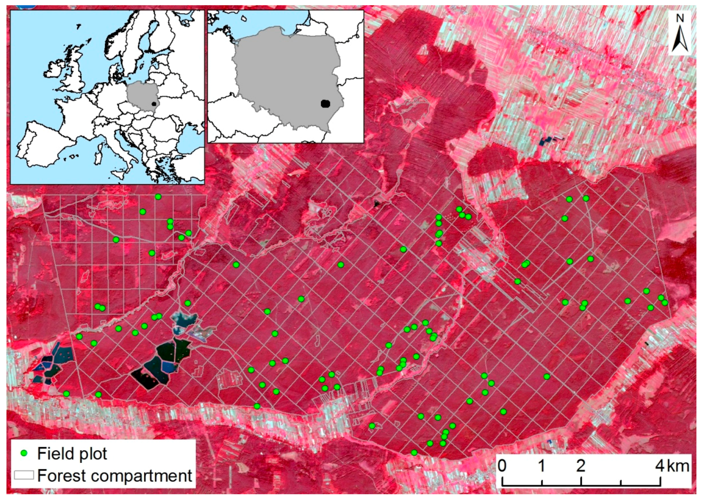
The study area is located in the South-Eastern Poland. The analyzed area of about 7800 ha of managed forest stands is owned by the Polish State Forest National Holding (Figure 1). The Scots pine (Pinus sylvestris L.) is the dominant tree species with a 95% share of the total stock. According to the forest inventory data provided by the Polish State Forest National Holding the average stand age is 67 years. The stands are generally even-aged and one layered.

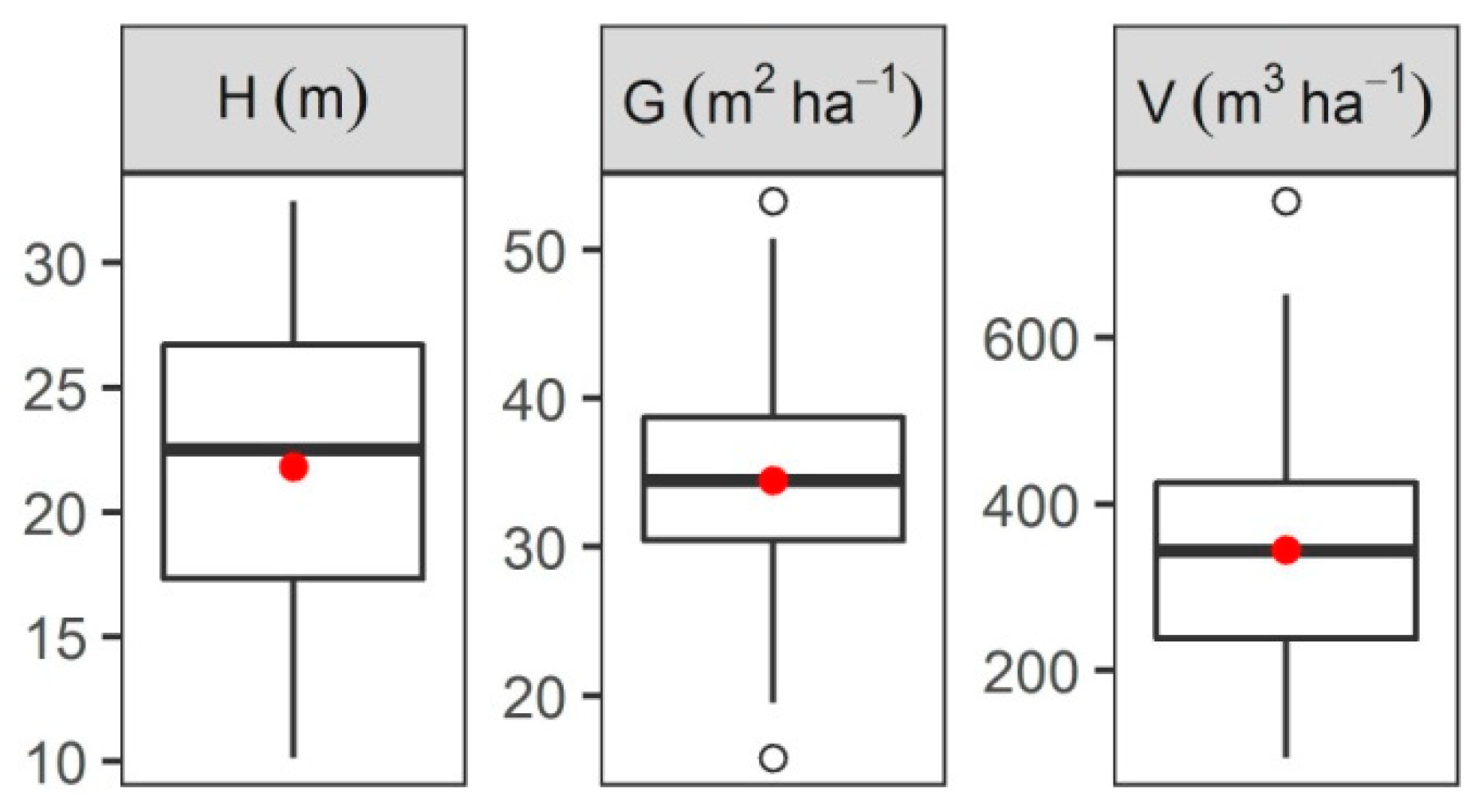
In order to capture the variability of the surveyed Scots pine stands, the field plot locations were selected via a pre-stratification method using three forest stand attributes: stand age, height and canopy cover. Stand age was obtained from an existing forest database. The ALS point clouds acquired on 19 October 2013 under leaf-on canopy conditions were used for stand height (95th percentile of normalized point heights) and canopy cover (percentage of first returns above 4 m) assessment. These two parameters were calculated with 20 m grid cells using FUSION (Version 3.42) software package [20]. Then, for the analyzed stand parameters the 20 m resolution raster layers were created with the following classes: four classes for stand age using a 25-year step and beginning at year 20; five classes for stand height using a 5 m step from a range of 10–35 m; and four classes for canopy cover using a 25% step. Then, a spatial combination of the three raster layers (age, height, canopy cover) was created giving the raster layer a value for each unique combination of input layers. Forest stands younger than 20 years and small strata with a total area <1.0 ha were excluded from analysis. This led to 47 unique strata. Finally, two plots were selected for each of the 47 strata using a stratified random sampling scheme that resulted in 94 field plots with an area of 400 m² (11.28 m radius). Field measurements were performed in August 2015. Plots were located in the field with sub-meter precision using a MobileMapper 120 (Spectra Precision) GNSS receiver. The diameter at breast height (DBH) and tree species on the plot were recorded for all standing trees with DBH ≥ 7.0 cm, whereas the height was measured only for three trees from the seven trees closest to the plot center at each inventory plot. The selected seven trees were ordered according to DBH, and the third, fourth and fifth trees were then measured for height. Subsequently, the height and volume for all DBH recorded trees were calculated based on empirical formula created for Scots pine in Poland [21]. Obtained measurements of Lorey’s mean height (H [m]), basal area (G [m²/ha]) and growing stock volume (V [m³/ha]) calculated from all trees at plot level are shown in Figure 2.

To achieve the intended research objectives three different types of remote sensing data were required: ALS point clouds, digital aerial images and Sentinel-2 satellite images.

The ALS point clouds acquired on 19 October 2013 under leaf-on canopy conditions were used for generating Digital Terrain Model (DTM_ALS) in the Polish coordinate system (PL-1992; EPSG-2180). The classified ALS point clouds (ver. 1.2; ASPRS, Bethesdan, MD, USA) with average density of 6.3 points·m⁻² were obtained from the Main Office of Geodesy and Cartography (GUGiK) in Warsaw (Poland). The 1.0 m spatial resolution DTM_ALS for the entire test area was generated using the FUSION (Version 3.42) software package [20].

Digital aerial images were collected with two separate flights performed on the 9 and 28 August 2015 using a UltraCamXp camera (Vexcel, Graz, Austria). The obtained Colour InfraRed (CIR) images had Ground Sampling Distance (GSD) of 0.25 m. In order to generate IPCs the PhotoScan Professional software package was used (version 1.3.4, Agisoft, Petersburg, Russia). The software exploits a computer vision Structure from Motion approach (SfM; [22]) for image matching and 3D point cloud generation [23,24]. The software parameters set for image processing in this study are given in

Table 1. Parameters used for processing of airborne images in Agisoft PhotoScan Professional software.

Processing Step	Parameter	Value
Align photos	Accuracy	High
	Pair pre-selection	Reference
	Key point limit	40,000
	Tie point limit	1000
Build dense cloud	Quality	High
	Depth filtering	Moderate

. The 11 Ground Control Points (GCPs) were used for calculation of external camera orientation (EO) and georeferencing. The coordinates of GCPs were obtained from an aerial orthophoto (2015) available through the Web Mapping Service: www.geoportal.gov.pl (XY coordinates; PL-1992 reference coordinate system) and from the DTM_ALS (Z coordinate; Kronsztadt 1986 elevation reference system). The achieved point cloud density amounted to 6.9 points/m². Subsequently, the IPCs were normalized using the DTM_ALS values by subtracting the point elevation from the ground elevation. In the next step, the IPCs were limited to the borders of each of the 94 inventory plot. Then, the selected point cloud metrics (

Table 2. Predictor variables obtained from image-derived point clouds (IPC).

Metric (Unit)	Description
Elev.mean (m)	Mean normalized height of points
Elev.mode (m)	Mode normalized height of points
Elev.stddev (m)	Standard deviation of normalized heights of points
Elev.CV	Coefficient of variation of normalized heights of points
Elev.IQ (m)	Interquartile distance of normalized heights of points
Elev.skewness	Skewness of normalized heights of points
Elev.kurtosis	Kurtosis of normalized heights of points
Elev.AAD (m)	Average absolute deviation from mean normalized height of points
Elev.P10, Elev.P25, Elev.P50, Elev.P75, Elev.P90, Elev.P95, Elev.P99 (m)	Percentiles of normalized heights of points: 10th, 25th, 50th, 75th, 90th, 95th, 99th
Canopy.relief.ratio	Canopy relief ratio = (Elev.mean − Elev.min)/(Elev.max − Elev.min)
Elev.L1, Elev.L2, Elev.L3, Elev.L4	L moments of normalized heights of points
Perc.all.ret.above.4.00 (%)	Percentage of points above 4 m above ground
Perc.all.ret.above.mean (%)	Percentage of points above mean normalized height
Perc.all.ret.above.mode (%)	Percentage of points above mode normalized height

) were calculated using FUSION software [20]. Only points with normalized height above the 1.0 m threshold were considered in the calculation in order to eliminate ground-related noise. Additionally, the 4.0 m height threshold was used for canopy density metrics calculation to select those points that represented the tree canopy heights only.

One cloud free Sentinel-2 scene acquired on 31th August (S2) was used in this study. The data were obtained from the Copernicus Open Access Hub (https://scihub.copernicus.eu/dhus/#/home) as Level-1C data with Top of Atmosphere (TOA) reflectance. Characteristics of the spectral bands of Sentinel-2 MSI (Multi-Spectral Instrument) sensor are presented in

Table 3. Spectral bands and resolutions of Sentinel-2 MSI sensor.

Band Number	Band Description	Wavelength Range (nm)	Resolution (m)
B1	Coastal aerosol	433–453	60
B2	Blue	458–523	10
B3	Green	543–578	10
B4	Red	650–680	10
B5	Red-edge 1	698–713	20
B6	Red-edge 2	733–748	20
B7	Red-edge	773–793	20
B8	Near infrared (NIR)	785–900	10
B8A	Near infrared narrow (NIRn)	855–875	20
B9	Water vapour	935–955	60
B10	Shortwave infrared/Cirrus	1360–1390	60
B11	Shortwave infrared 1 (SWIR1)	1565–1655	20
B12	Shortwave infrared 2 (SWIR2)	2100–2280	20

. The atmospheric correction of Level-1C input data was performed using the Sen2Cor plug-in for Sentinel-2 Toolbox and SNAP software provided by ESA (version 6.0.0, Brockmann Consult, Geesthacht, Germany). The obtained Bottom of Atmosphere (BOA) surface reflectance images were resampled to 10 m spatial resolution. In the case of B5, B6, B7 and B8A spectral bands this resulted in four identical surface reflectance values at 10 m pixel size. All spectral bands except B1, B9 and B10, were used for building the predictive models. Finally, the mean surface reflectance values for BOA bands were calculated for each inventory plot. The calculated mean value was weighted by the fraction of each pixel that was covered by the field plot. These mean values were subsequently used as predictor variables in regression models.

Multiple linear regression (LM) and random forest (RF; [25]) methods were used to create predictive models of growing stock volume (V). The models were created from three sets of predictor variables: reflectance values of Sentinel-2 images acquired in August 2015 (S2), IPC metrics (IPC), and a combination of selected IPC metrics and Sentinel-2 reflectance values (IPC.S2). To reduce the number of models for evaluation only those metrics selected in the final IPC.LM model were added to the IPC.S2 predictor set. First, the non-collinear variables were selected from each set of metrics separately. For a pair of analyzed predictors with a Spearman correlation higher than 0.9, the one with the lower correlation with V was dropped. Subsequently, a 2^k number of LM models were created for each predictor set, where k is the number of variables in a certain set. This enabled evaluation of LM models with all possible combinations of pre-selected predictor variables within one predictor set. The best model within each predictor set and regression method (LM, RF) was selected based on the lowest value of root mean squared error (RMSE). The RF approach has a tuning parameter called mtry which is the number of randomly selected predictors, to choose from at each split [25,26]. For the purpose of tuning the mtry parameter the sequence of integers across the range from 2 to the number of predictors in each predictor set was used. For each RF model all non-correlated variables within the variable set were used. The number of trees for the forest was set to 1000 in all models.

Models accuracy was assessed using a bootstrap method with 500 repetitions [27]. The observations not used in a certain repetition for model training were used for assessment of the model performance (hold-out set). Measures of the models’ accuracy were obtained using the R², RMSE and Bias. These were calculated using the following equations:

$${\mathrm{R}}^2=\frac{{\displaystyle \sum {({\widehat{y}}_i-\overline{y})}^2}}{{\displaystyle \sum {(y_i-\overline{y})}^2}}$$

(1)

$$\mathrm{RMSE}=\sqrt{\frac{{\displaystyle \sum {(y_i-{\widehat{y}}_i)}^2}}{n}}$$

(2)

$$\mathrm{Bias}=\frac{{\displaystyle \sum (y_i-{\widehat{y}}_i)}}{n}$$

(3)

where:

• $y_i$ = observed growing stock volume for the ith sample plot in a hold-out set,
• ${\widehat{y}}_i$ = predicted growing stock volume for the ith sample plot in the hold-out set,
• $\overline{y}$ = mean of n observed values in the hold-out set,
• n = number of observations in the hold-out set.

Obtained performance parameters were subsequently averaged over the 500 bootstrap iterations. The averaged RMSE and Bias were then divided by the mean value of V and multiplied by 100% to create RMSE% and Bias%, respectively. Additionally, an inferential assessment of model performance was performed using the “diff” function from the caret R package [28]. The ideas and method of this tool are based on benchmark experiment design [29,30]. Benchmark studies are aimed at comparing the performance of several competing algorithms for a certain learning problem. The general idea is that using a proper resampling scheme (e.g., bootstrap) the resulting performance observations are independent and identically distributed. Thus, the performance of predictive models can be compared using standard statistical test procedures to test hypotheses about the distribution of the performance measures. In our study, the pair-wise differences between the models’ RMSE and R² from 500 bootstrap runs were computed and tested with Paired Student’s t-test to assess if the difference is equal to zero (α = 0.05). For a single bootstrap run the same hold-out observations were used for each evaluated model.

To assess the robustness of predictor variables we used different approaches for LM and RF models. In the case of LM, the relative variable importance (RVI) was assessed based on Akaike weights [31]. The RVI was calculated as the sum of the Akaike weights in the subset of models including that predictor. The calculation was performed separately for each set of predictors (S2, IPC and IPC.S2) for all possible combinations of variables. Calculation of variable importance for LM was performed using the R “AICcmodavg” package [32].

For RF models, the RVI of variables was assessed using the approach implemented in the “randomForest” R package [33]. The calculation of variable importance was performed in each predictor set for the optimal model in terms of the mtry parameter. The idea behind this method is that the Mean Squared Error (MSE) calculated for a single tree on the out-of-bag portion of the data is compared to the MSE of the same tree obtained after permutation of each predictor variable. The difference between these two MSE values are subsequently averaged over all trees, and normalized by the standard error. For easier comparison between RVI values obtained for LM and RF methods the variable importance values from RF models were scaled to have a maximum value of 1.

3. Results

3.1. Predictor Variables Pre-Selection

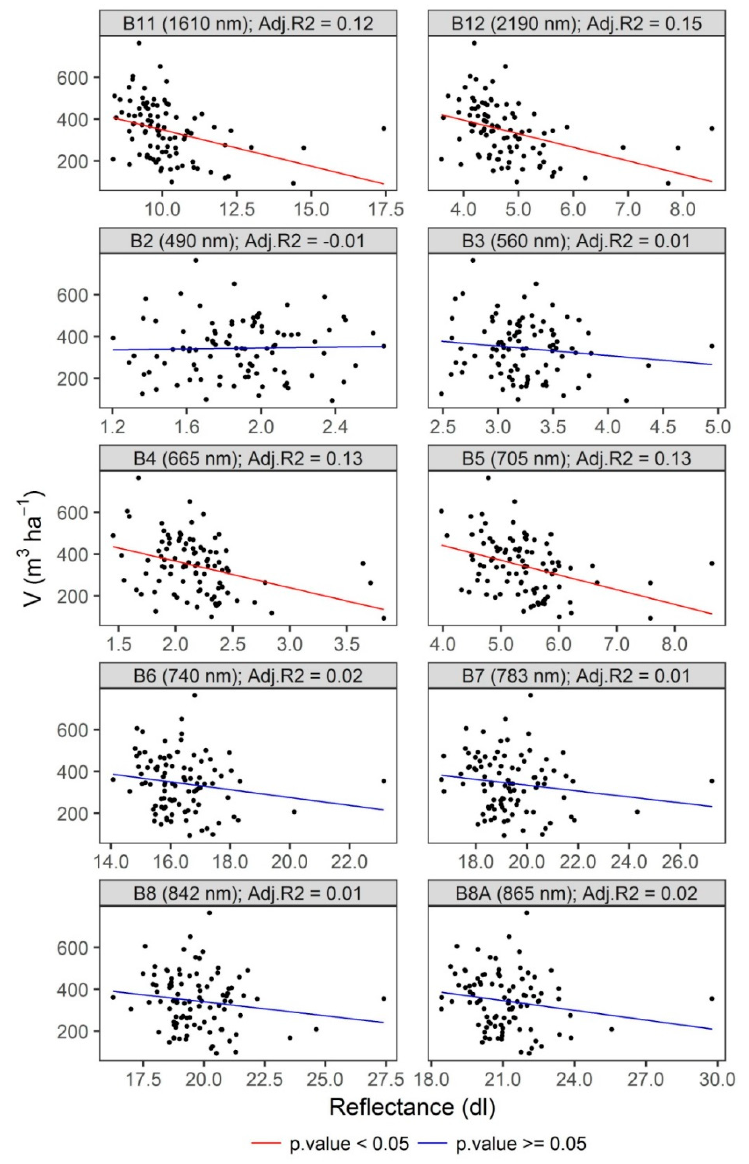
The Spearman correlation coefficient values describing the correlation between V and evaluated predictor variables are showed in

Table 4. The Spearman correlation coefficient (r_S) values between V and evaluated IPC metrics (* correlation is significant at the 0.05 level).

IPC Metrics	rS
Elev.mean	0.91 *
Elev.L1	0.91 *
Elev.P25	0.90 *
Elev.P50	0.89 *
Elev.mode	0.88 *
Elev.P75	0.87 *
Elev.P80	0.87 *
Elev.P10	0.86 *
Elev.P90	0.86 *
Elev.P95	0.86 *
Elev.P99	0.84 *
Elev.CV	−0.39 *
Perc.all.ret.above.4.00	0.24 *
Elev.L4	0.23 *
Elev.stddev	0.17
Elev.AAD	0.17
Elev.L2	0.17
Elev.IQ	0.14
Elev.kurtosis	0.12
Perc.all.ret.above.mode	0.08
Canopy.relief.ratio	0.07
Elev.L3	−0.04
Elev.skewness	−0.01
Perc.all.ret.above.mean	−0.01

and

Table 5. The Spearman correlation coefficient (r_S) values between V and evaluated Sentinel-2 spectral bands (* correlation is significant at the 0.05 level).

S2 Bands	rS
B12	−0.51 *
B11	−0.46 *
B5	−0.41 *
B4	−0.39 *
B8A	−0.24 *
B6	−0.21 *
B7	−0.20
B8	−0.17
B3	−0.10
B2	0.05

. The variable Elev.mean was found to have the highest correlation with V (r_S = 0.91). Also high correlations were found between V and elevation percentiles of point cloud. It is worth noting that the elevation percentiles were highly correlated with Elev.mean, therefore, they were not used in the next steps for creating predictive models. In the case of Sentinel-2 reflectance values, the highest correlations with V were observed for B12 (r_S = −0.51) and B11 (r_S = −0.46) bands while the lowest with B2 (r_S = 0.05). The scatterplots of growing stock volume (V) at plot level versus Sentinel-2 reflectance values are presented in Figure 3. For most Sentinel-2 spectral bands the relationship between V and reflectance values was negative (Figure 3; Table 5). Removing highly correlated predictors lead to a reduction in the number of models for evaluation. The highest number of models were evaluated for the IPC.S2 predictor set (512). The optimal value of the mtry tuning parameter varied from 2 for S2.RF to 8 for the IPC.RF model (

Table 6. Results of removing highly correlated predictors within variable sets. The number of evaluated models in each predictor set and final mtry values used in RF are also given (* predictors selected in the final LM models).

Predictor Variable Set	Predictors	Number of Evaluated LM Models	Number of Evaluated RF Models	mtry Value of the Final RF Model
S2	B2 *, B3, B4 *, B5, B8A, B12	64	5	2
IPC	Elev.mean *, Elev.stddev, Elev.CV, Elev.skewness, Elev.kurtosis, Elev.L4, Canopy.relief.ratio *, Perc.all.ret.above.mean, Perc.all.ret.above.mode	512	8	8
IPC.S2	Elev.mean *, Canopy.relief.ratio *, B2 *, B3 *, B4, B5, B8A *, B12	256	7	7

).

3.2. Performance of Predictive Models of Growing Stock Volume

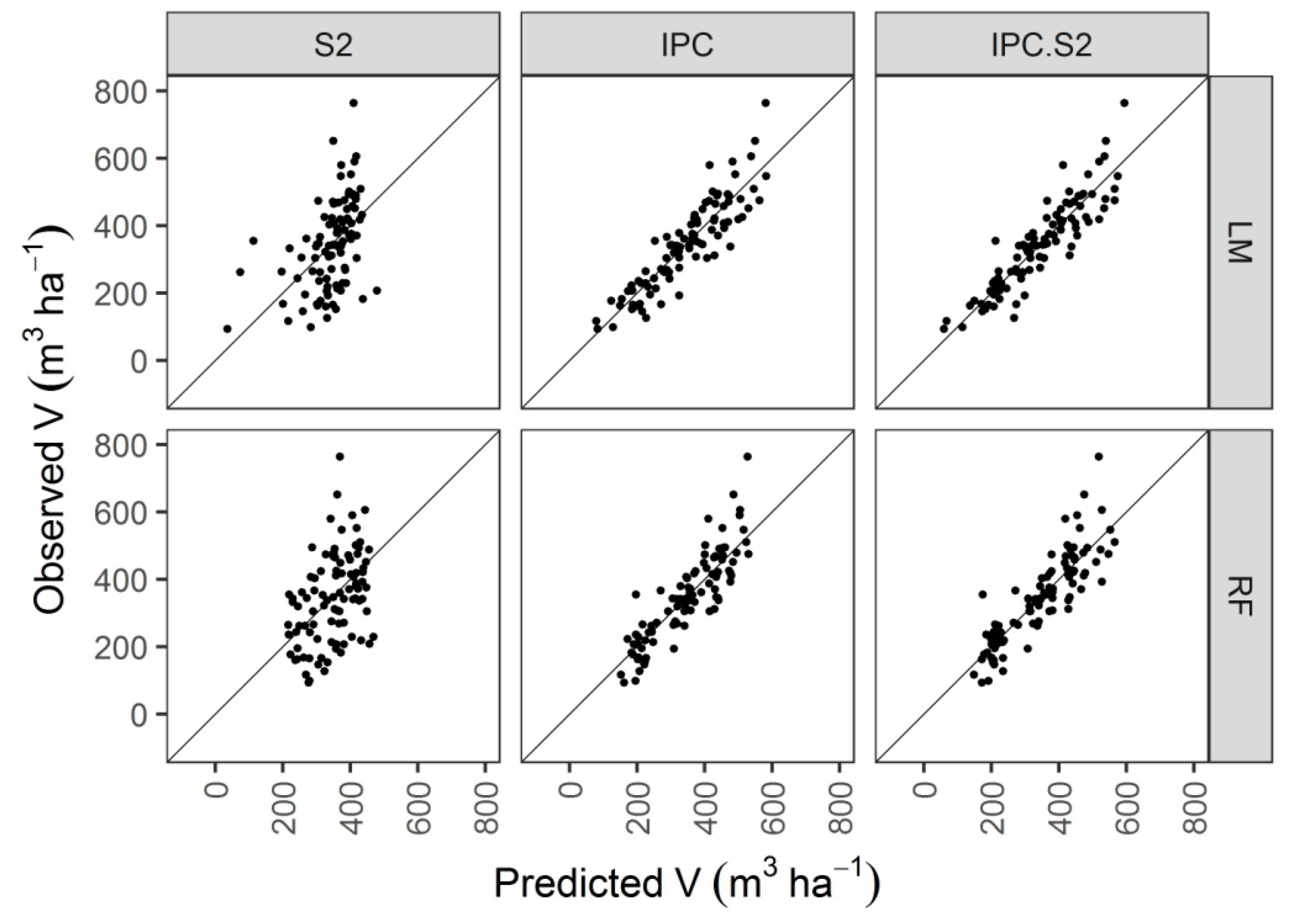
The 6 growing stock volume (V) predictive models were created based on predictor variables obtained from spectral bands of Sentinel-2 images and IPC metrics, using two regression methods (LM and RF). The relationships between observed and predicted values of V obtained from bootstrap resampling are presented in Figure 4.

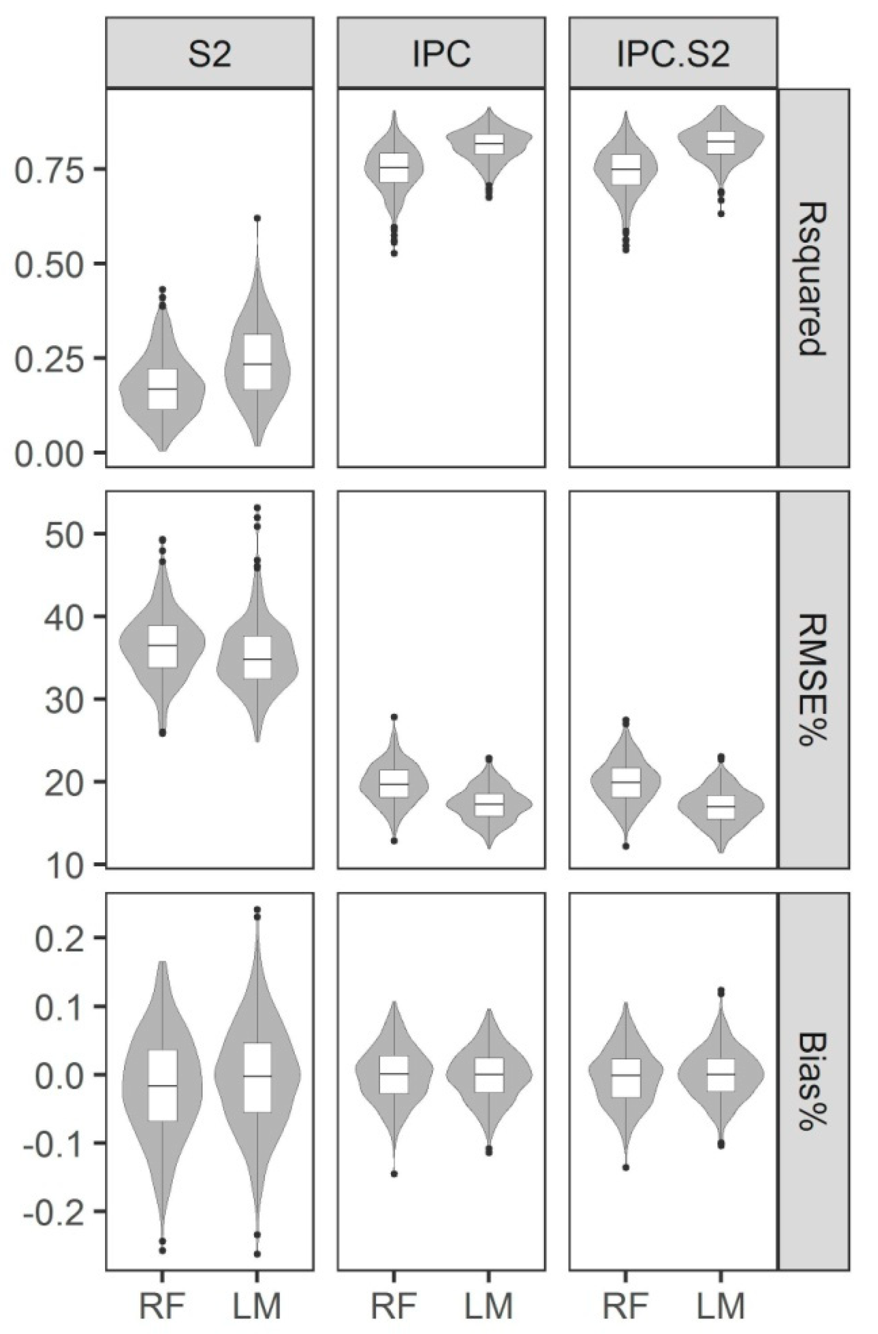
Averaged R², RMSE, RMSE%, Bias and Bias% values for the created predictive models are presented in

Table 7. Averaged R², RMSE, RMSE%, bias and bias% values for the analyzed models and regression method.

Metric	Model	Regression Method
		RF	LM
R2	S2	0.17	0.24
	IPC	0.75	0.81
	IPC.S2	0.75	0.82
RMSE	S2	124.89	120.37
	IPC	67.73	59.18
	IPC.S2	68.58	58.14
RMSE%	S2	36.46	35.14
	IPC	19.73	17.26
	IPC.S2	19.98	16.95
Bias	S2	−4.72	−0.10
	IPC	0.69	0.09
	IPC.S2	−0.72	0.33
Bias%	S2	−0.02	0.00
	IPC	0.00	0.00
	IPC.S2	0.00	0.00

. Additionally, the distribution of the selected performance metrics (R², RMSE%, Bias%) from the 500 bootstrap runs are presented in Figure 5. The best model was achieved using LM based on the IPC combined with the Sentinel-2 image, with RMSE%_IPC.S2.LM = 16.95% and R²_IPC.S2.LM = 0.82. The LM regression method created more accurate models than the RF method in all predictor variable sets. The bias was close to 0 for all constructed models. The poorest model was obtained with the RF method based on S2 data, with RMSE%_S2.RF = 36.46% and R²_S2.RF = 0.17. The largest difference in R² was observed between the IPC.S2.LM and the S2.RF models (0.65). The difference in RMSE was also highest for this pair of analyzed models. Inferential assessment of model performance showed that the differences in accuracy in terms of R² and RMSE were statistically significant (α = 0.05) for all pairs of models excepting the IPC.S2.RF and IPC.RF pair. The results of the inferential assessment of the models’ differences in terms of R² are presented in

Table 8. Results of inferential assessment of model performance differences in terms of R². The pair-wise differences between the models R² from 500 bootstrap runs were tested with Paired Student’s t-test (α = 0.05). The upper diagonal shows the estimates of the difference. The lower diagonal shows the p-value for H0: difference = 0.

Model	S2.LM	IPC.LM	IPC.S2.LM	S2.RF	IPC.RF	IPC.S2.RF
S2.LM		−0.573	−0.579	0.065	−0.510	−0.505
IPC.LM	<2.2 × 10−16		−0.007	0.638	0.062	0.067
IPC.S2.LM	<2.2 × 10−16	4.877 × 10−6		0.645	0.069	0.074
S2.RF	<2.2 × 10−16	<2.2 × 10−16	<2.2 × 10−16		−0.576	−0.570
IPC.RF	<2.2 × 10−16	<2.2 × 10−16	<2.2 × 10−16	<2.2 × 10−16		0.005
IPC.S2.RF	<2.2 × 10−16	<2.2 × 10−16	<2.2 × 10−16	<2.2 × 10−16	0.074

.

3.3. Relative Variable Importance

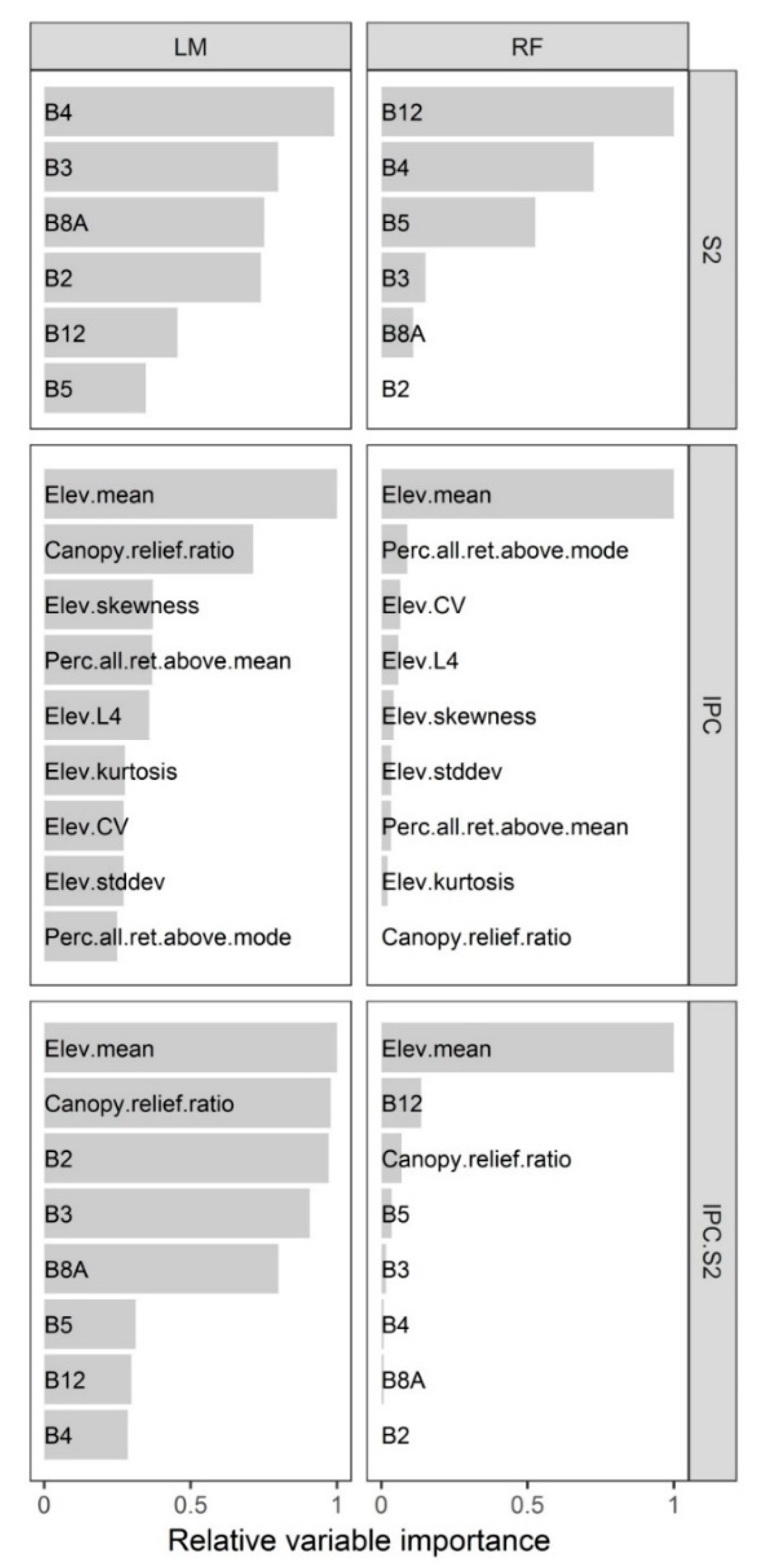
Analysis of relative variable importance showed that depending on the applied regression method, LM or RF, different predictor variables were found to be most robust (Figure 6). Only the Elev.mean variable showed the highest RVI value for both regression methods (IPC and IPC.S2 variable sets). In case of IPC-based models the Canopy.relief.ratio was found to be a robust predictor variable for the LM but not for the RF approach. In Sentinel-2-based models, B4 was shown to be an important predictor for both, the LM and the RF methods.

4. Discussion

The two main goals of this study were to evaluate the suitability of Sentinel-2 reflectance values for estimating the growing stock volume (V) of single layer Scots pine stands and to analyze whether the Sentinel-2 imagery can improve the accuracy of IPC-based predictive models. We also examined the accuracy of two different regression methods—multiple linear regression (LM) and random forest (RF) and analyzed the robustness of variables used in created predictive models. As far as we know, this is the first time that fusion of Sentinel-2 satellite images and IPC data has been examined in the context of growing stock volume estimation of Scots pine stands.

Our results indicate that Sentinel-2-based predictive models estimates the growing stock volume (V) of Scots pine stands with low accuracy. It is worth noting that although additional use of Sentinel-2 imagery in the IPC-based predictive model provided a statistically significant increase in accuracy, the increase was relatively low (0.01 increase in R² and 0.31% decrease in RMSE%). The obtained results show that a multiple linear (LM) regression approach provides a more accurate growing stock volume (V) estimation of single layer Scots pine stands than the random forest (RF) method when using IPC and Sentinel-2 datasets. The results show that different predictor variables may be optimal for constructing growing stock volume models of Scots pine stands depending on the applied regression method—LM or RF.

The results obtained for growing stock volume estimation using IPC data (RMSE%_IPC.LM = 17.26%) are consistent with our previous findings for the same reference dataset but with different aerial images (RMSE% = 17.0%; [34]). The obtained accuracies of IPC-based predictive models also concur well with findings from previous experiments performed by other authors in similar forest stand conditions [8,35]. Regarding the effectiveness of IPC metrics for V estimation using LM, the Elev.mean and Canopy.relief.ratio were found to be the most robust predictor variables which is consistent with previous results obtained for this study area [34].

Our results regarding the suitability of Sentinel-2 spectral bands for growing stock volume (V) estimation are similar to findings from a previous study on AGB estimation based on Seninel-2 simulated bands [5]. The relationships between all ratio vegetation indices (RVI) and normalized difference vegetation indices (NVI) and AGB were analyzed. It was also found that none of the band combinations showed strong relationships with AGB. The highest R² values were achieved using RVI band combination B6 (or B7, B8A, B8 or B9)/B11 (R² = 0.24) [5].

Sentinel-2-based predictive models of V had lower accuracy than those reported for Mediterranean forest ecosystems [4]. In our study the coefficient of determination of the best Sentinel-2-based model amounted to R²_S2.LM = 0.24, while authors studying Mediterranean forests achieved R² = 0.63 (RF method). In the above-mentioned study, bands B11 and B6 were found to be most effective in estimating V with R² = 0.46 and 0.38, respectively. In our study, in the case of two RF models, the SWIR bands (B11 and B12) were also found to be useful for V estimation. In contrast to previous studies [4] we did not use the B6 band, because it was correlated with the B8A band. Surprisingly, we found the B2 band to be a useful predictor of V in the case of the IPC.S2 variable set. This finding is in contrast with previous results reported in the literature [4,36]. There are also known results of using Sentinel-2 imagery for estimation of V in broadleaf forests in Italy. It was found that using k-NN imputation algorithm based on an RF distance matrix the V can be estimated with a relative root mean squared difference ranging from 11.36% to 26.05% for two different study areas [6]. These results are difficult to compare with those obtained in [4] and in this study since different modeling methods were used. There are also known results where different S2 bands were found to be most robust for two different study areas: B8, B11, B12 and B5, B6, B8 [6]. In our study different sets of best S2 bands were also identified depending on the regression method (LM, RF). This suggests that the robustness of S2 spectral bands in the estimation of V should always be analyzed for each particular case.

Another study evaluating the suitability of Sentinel-2 imagery for growing stock volume estimation was performed in Norway spruce (Picea abies (L.) H. Karst.) dominated stands in Germany [37]. In that study the high-resolution airborne hyperspectral HyMap dataset was used to simulate the Sentinel-2 satellite data. Using the K-nearest neighbor algorithm the authors created a V predictive model with an RMSE% = 21.58% at stand level.

Given that our study was performed on almost single species stands, the general conclusions about the relatively low usability of Sentinel-2 satellite imageries for growing stock volume (V) estimation of Scots pine stands are formulated with considerable caution. It is possible that in stands composed of more diverse tree species, the incorporation of Sentinel-2 reflectance values into IPC-based predictive models might lead to higher accuracy than was found in the present study. Our study might be limited because we did not report the predictive power of common Vegetation Indices (VI) for V estimation. However, there is evidence from previous studies [4,38] that VI may be less correlated to forest stand parameters compared to the original spectral bands. For that reason, and because we wanted to use a more straightforward approach, we decided not to analyze the usability of VI for growing stock volume estimation in this study.

Our findings suggest that multiple linear regression is a more powerful regression method than random forest for V estimation in Scots pine stands. However, it should be kept in mind that these findings apply only to the described study area and a specific set of predictor variables. Despite this, we believe that examining the performance of traditional statistical methods like linear regression before deciding to use more advanced methods such as random forest is important and worthwhile. We are aware that in more complex forest stands with a nonlinear relationship between growing stock volume and predictor variables, the RF method may surpass the LM approach.

5. Conclusions

The presented study investigated whether the reflectance values of Sentinel-2 satellite images can be used to estimate growing stock volume for single canopy layer Scots pine dominated stands. This is one of the first studies aimed at enhancing our understanding of the usability of Sentinel-2 satellite images for growing stock volume estimation. Our results indicate that Sentinel-2-based predictive models demonstrate low accuracy in estimating the growing stock volume of Scots pine stands. Inclusion of Sentinel-2 reflectance values into predictive models created from airborne image-derived point cloud metrics does not significantly improve the accuracy of the model. Our findings could be useful for practitioners to decide whether additional utilization of Sentinel-2 images into IPC-based models is justified from an operational point of view. This work shows that multiple linear regression methods may provide more accurate predictive models than random forest methods in the context of growing stock volume estimation of single layer Scots pine stands when using airborne image-derived point clouds and Sentinel-2 reflectance values.

References

- White, J.C.; Coops, N.C.; Wulder, M.A.; Vastaranta, M.; Hilker, T.; Tompalski, P. Remote Sensing Technologies for Enhancing Forest Inventories: A Review. Can. J. Remote Sens. 2016, 42, 619–641. [Google Scholar] [CrossRef]
- Maltamo, M.; Naesset, E.; Vauhkonen, J. Forestry Applications of Airborne Laser Scanning. Concepts and Case Studies; Maltamo, M., Naesset, E., Vauhkonen, J., Eds.; Springer: Berlin, Germany, 2014. [Google Scholar]
- Drusch, M.; Del Bello, U.; Carlier, S.; Colin, O.; Fernandez, V.; Gascon, F.; Hoersch, B.; Isola, C.; Laberinti, P.; Martimort, P.; et al. Sentinel-2: ESA’s Optical High-Resolution Mission for GMES Operational Services. Remote Sens. Environ. 2012, 120, 25–36. [Google Scholar] [CrossRef]
- Chrysafis, I.; Mallinis, G.; Siachalou, S.; Patias, P. Assessing the relationships between growing stock volume and Sentinel-2 imagery in a Mediterranean forest ecosystem. Remote Sens. Lett. 2017, 8, 508–517. [Google Scholar] [CrossRef]
- Majasalmi, T.; Rautiainen, M. The potential of Sentinel-2 data for estimating biophysical variables in a boreal forest: A simulation study. Remote Sens. Lett. 2016, 7, 427–436. [Google Scholar] [CrossRef]
- Mura, M.; Bottalico, F.; Giannetti, F.; Bertani, R.; Giannini, R.; Mancini, M.; Orlandini, S.; Travaglini, D.; Chirici, G. Exploiting the capabilities of the Sentinel-2 multi spectral instrument for predicting growing stock volume in forest ecosystems. Int. J. Appl. Earth Obs. Geoinf. 2018, 66, 126–134. [Google Scholar] [CrossRef]
- White, J.; Wulder, M.; Vastaranta, M.; Coops, N.; Pitt, D.; Woods, M. The Utility of Image-Based Point Clouds for Forest Inventory: A Comparison with Airborne Laser Scanning. Forests 2013, 4, 518–536. [Google Scholar] [CrossRef]
- Yu, X.; Hyyppä, J.; Karjalainen, M.; Nurminen, K.; Karila, K.; Vastaranta, M.; Kankare, V.; Kaartinen, H.; Holopainen, M.; Honkavaara, E.; et al. Comparison of laser and stereo optical, SAR and InSAR point clouds from air- and space-borne sources in the retrieval of forest inventory attributes. Remote Sens. 2015, 7, 15933–15954. [Google Scholar] [CrossRef]
- White, J.; Stepper, C.; Tompalski, P.; Coops, N.; Wulder, M. Comparing ALS and Image-Based Point Cloud Metrics and Modelled Forest Inventory Attributes in a Complex Coastal Forest Environment. Forests 2015, 6, 3704–3732. [Google Scholar] [CrossRef]
- Rahlf, J.; Breidenbach, J.; Solberg, S.; Næsset, E.; Astrup, R. Comparison of four types of 3D data for timber volume estimation. Remote Sens. Environ. 2014, 155, 325–333. [Google Scholar] [CrossRef]
- Pitt, D.G.; Woods, M.; Penner, M. A Comparison of Point Clouds Derived from Stereo Imagery and Airborne Laser Scanning for the Area-Based Estimation of Forest Inventory Attributes in Boreal Ontario. Can. J. Remote Sens. 2014, 40, 214–232. [Google Scholar] [CrossRef]
- Maack, J.; Lingenfelder, M.; Weinacker, H.; Koch, B. Modelling the standing timber volume of Baden-Württemberg—A large-scale approach using a fusion of Landsat, airborne LiDAR and National Forest Inventory data. Int. J. Appl. Earth Obs. Geoinf. 2016, 49, 107–116. [Google Scholar] [CrossRef]
- Shataee, S. Forest attributes estimation using aerial laser scanner and TM data. For. Syst. 2013, 22, 484–496. [Google Scholar] [CrossRef]
- Tonolli, S.; Dalponte, M.; Neteler, M.; Rodeghiero, M.; Vescovo, L.; Gianelle, D. Fusion of airborne LiDAR and satellite multispectral data for the estimation of timber volume in the Southern Alps. Remote Sens. Environ. 2011, 115, 2486–2498. [Google Scholar] [CrossRef]
- Jiménez, E.; Vega, J.A.; Fernández-Alonso, J.M.; Vega-Nieva, D.; Ortiz, L.; Lopez-Serrano, P.M.; López-Sánchez, C.A. Estimation of aboveground forest biomass in Galicia (NW Spain) by the combined use of LiDAR, LANDSAT ETM+ and national forest inventory data. IForest 2017, 10, 590–596. [Google Scholar] [CrossRef]
- Dash, J.P.; Watt, M.S.; Bhandari, S.; Watt, P. Characterising forest structure using combinations of airborne laser scanning data, RapidEye satellite imagery and environmental variables. Forestry 2016, 89, 159–169. [Google Scholar] [CrossRef]
- Phua, M.H.; Johari, S.A.; Wong, O.C.; Ioki, K.; Mahali, M.; Nilus, R.; Coomes, D.A.; Maycock, C.R.; Hashim, M. Synergistic use of Landsat 8 OLI image and airborne LiDAR data for above-ground biomass estimation in tropical lowland rainforests. For. Ecol. Manag. 2017, 406, 163–171. [Google Scholar] [CrossRef]
- Sivanpillai, R.; Smith, C.T.; Srinivasan, R.; Messina, M.G.; Wu, X. Ben Estimation of managed loblolly pine stand age and density with Landsat ETM+ data. For. Ecol. Manag. 2006, 223, 247–254. [Google Scholar] [CrossRef]
- Korhonen, L.; Hadi; Packalen, P.; Rautiainen, M. Comparison of Sentinel-2 and Landsat 8 in the estimation of boreal forest canopy cover and leaf area index. Remote Sens. Environ. 2017, 195, 259–274. [Google Scholar] [CrossRef]
- McGaughey, R.J. FUSION/LDV: Software for LIDAR Data Analysis and Visualization; USDA Forest Service, Pacific Northwest Research Station: Seattle, WA, USA, 2015. [Google Scholar]
- Bruchwald, A.; Rymer-Dudzińska, T.; Dudek, A.; Michalak, K.; Wróblewski, L.; Zasada, M. Wzory empiryczne do określania wysokości i pierśnicowej liczby kształtu grubizny drzewa. Sylwan 2000, 144, 5–12. [Google Scholar]
- Turner, D.; Lucieer, A.; Watson, C. An automated technique for generating georectified mosaics from ultra-high resolution Unmanned Aerial Vehicle (UAV) imagery, based on Structure from Motion (SFM) point clouds. Remote Sens. 2012, 4, 1392–1410. [Google Scholar] [CrossRef]
- Dandois, J.P.; Ellis, E.C. High spatial resolution three-dimensional mapping of vegetation spectral dynamics using computer vision. Remote Sens. Environ. 2013, 136, 259–276. [Google Scholar] [CrossRef]
- Turner, D.; Lucieer, A.; Wallace, L. Direct Georeferencing of Ultrahigh-Resolution UAV Imagery. IEEE Trans. Geosci. Remote Sens. 2014, 52, 2738–2745. [Google Scholar] [CrossRef]
- Breiman, L. Random Forests. Mach. Learn. 2001, 45, 5–32. [Google Scholar] [CrossRef]
- Kuhn, M.; Johnson, K. Applied Predictive Modeling; Springer: New York, NY, USA, 2013; ISBN 1461468485. [Google Scholar]
- Efron, B.; Tibshirani, R. Bootstrap Methods for Standard Errors, Confidence Intervals, and Other Measures of Statistical Accuracy. Stat. Sci. 1986, 1, 54–75. [Google Scholar] [CrossRef]
- Caret: Classification and Regression Training. Available online: https://cran.r-project.org/web/packages/caret/index.html (accessed on 29 March 2018).
- Hothorn, T.; Leisch, F.; Zeileis, A.; Hornik, K. The Design and Analysis of Benchmark Experiments. J. Comput. Graph. Stat. 2005, 14, 675–699. [Google Scholar] [CrossRef]
- Eugster, M.J.A.; Hothorn, T.; Leisch, F. Exploratory and Inferential Analysis of Benchmark Experiments; Technical Report, Number 030 2008; Department of Statistic, Ludwigs-Maximilians-Universitat Munchen: Munich, Germany, 2008. [Google Scholar]
- Burnham, K.P.; Anderson, D.R. Model Selection and Multimodel Inference, 2nd ed.; A Practical Information-Theoretic Approach; Springer: Berlin, Germany, 2002. [Google Scholar]
- AICcmodavg: Model Selection and Multimodel Inference Based on (Q)AIC(c). Available online: https://cran.r-project.org/web/packages/AICcmodavg/index.html (accessed on 30 March 2018).
- Liaw, A.; Wiener, M. Classification and Regression by randomForest. R News 2002, 2, 18–22. [Google Scholar]
- Hawryło, P.; Tompalski, P.; Wężyk, P. Area-based estimation of growing stock volume in Scots pine stands using ALS and airborne image-based point clouds. Forestry 2017, 90, 686–696. [Google Scholar] [CrossRef]
- Vastaranta, M.; Wulder, M.A.; White, J.C.; Pekkarinen, A.; Tuominen, S.; Ginzler, C.; Kankare, V.; Holopainen, M.; Hyyppä, J.; Hyyppä, H. Airborne laser scanning and digital stereo imagery measures of forest structure: Comparative results and implications to forest mapping and inventory update. Can. J. Remote Sens. 2013, 39, 382–395. [Google Scholar] [CrossRef]
- Mallinis, G.; Koutsias, N.; Makras, A.; Karteris, M. Forest parameters estimation in a European Mediterranean landscape using remotely sensed data. For. Sci. 2004, 50, 450–460. [Google Scholar]
- Nink, S.; Hill, J.; Buddenbaum, H.; Stoffels, J.; Sachtleber, T.; Langshausen, J. Assessing the suitability of future multi- and hyperspectral satellite systems for mapping the spatial distribution of norway spruce timber volume. Remote Sens. 2015, 7, 12009–12040. [Google Scholar] [CrossRef]
- Lu, D.; Mausel, P.; Brondízio, E.; Moran, E. Relationships between forest stand parameters and Landsat TM spectral responses in the Brazilian Amazon Basin. For. Ecol. Manag. 2004, 198, 149–167. [Google Scholar] [CrossRef]
Figure 1.
Location of the study area with 94 field plots established using stratified random sampling.
Figure 2.
Obtained measurements of H, G and V at plot level (minimum, first quartile, median, third quartile, and maximum; mean value is marked as the red point).
Figure 3.
Relationships between growing stock volume (V) at plot level and Sentinel-2 surface reflectance dimensionless (dl) values used as predictor variables (band center wavelength in nm is given in brackets). Adj.R2 is the Adjusted R-squared.
Figure 4.
Observed versus predicted growing stock volume for different predictor variable sets and regression methods. Predicted values are averaged from 500 bootstrap runs.
Figure 5.
Accuracies of the growing stock volume models created using RF and LM in terms of R2, RMSE% and Bias%. Violin- and box-plots display distribution of the results from the 500 bootstrap runs.
Figure 6.
Relative variable importance obtained for LM and RF regression methods within each predictor set.