Design-Unbiased Estimation and Alternatives for Sampling Trees on Plantation Rows

Abstract

Recently, methods for inventories of forest plantations have been proposed based on the use of remote sensing to estimate total row length, followed by the estimation of plantation row attributes, such as number and volume or weight of trees, at randomly selected field locations on the ground within a forest plantation of interest. While we are aware of instances in which such inventories have been performed, to our knowledge, no scientific studies of this approach have previously appeared. Many plantation inventories have been performed by traditional methods, such as Bitterlich (point) sampling and fixed-size plot sampling. Random plot sizes including a fixed number of rows are possible but the resulting estimators are typically not unbiased. Plot sampling and Bitterlich sampling can be problematic in plantations because inventory crews may gravitate towards the establishment of sample points in similar locations relative to row spacing, e.g., midway between rows, compromising the assumption of random point location in the tract area. We propose and test five novel estimators which are based on sampling a fixed number of trees at random sample locations on rows. The methods we propose can be used to estimate tract-level quantities of any tree attribute, including the number of trees, total volume, basal area, and others. Fixed row lengths may be sampled at randomly determined field locations on rows. Alternatively, distance sampling methods can be used to sample a fixed number of trees subsequent to, or nearest to, a randomly located point on a plantation row. Ducey’s recently-developed estimator for point-to-particle sampling on lines can be applied to sampling on rows. A “mean of ratios” (MR) estimator can be based on the average ratio of the sum of the sample trees’ attributes divided by the length of line occupied by the sample trees. A “ratio of means” (RM) estimator can be based on the ratio of the mean of the sample trees’ attributes for all random points divided by the mean sample line length for all random points. For either of these ratio estimators, the line length may be chosen to include the gap between trees into which the random sample point falls (G-MR, mean of ratios including the sample gap and G-RM, ratio of means estimator including the sample gap), or it may be chosen to begin subsequent to that gap (NG-MR, mean of ratios not including the sample gap and NG-RM, ratio of means not including the sample gap). A simulation was used to test each of these techniques on typical plantation row populations. Two row populations were used in the simulation. One had relatively uniform spacing between trees on a row, which resembles the characteristics of young plantations. The second population contained numerous gaps, typical of more mature plantations that have been thinned and may be experiencing mortality. In the simulations, the estimators were used to estimate the number of trees in each population. Trends in other variables, such as volume or basal area, were similar to those for te estimated number of trees in the populations. The simulation results showed that the G-MR method had the smallest root mean square error followed by the NG-RM. Ducey’s method and the fixed-length row plot were both design-unbiased. Both the latter methods had low root mean square errors but these were slightly higher than some of the other methods. In contrast to the other methods tested, the NG-MR and G-RM methods were both substantially biased on a simulated row population containing large gaps which might occur due to mortality or thinning. The estimators which had good performance in simulations—Ducey’s method, G-MR, NG-RM, and fixed-length row sampling—are viable alternatives to traditional methods of sampling plantations, such as Bitterlich sampling and fixed-size plot sampling, if accurate plantation row lengths can be measured.

1. Introduction

A design-unbiased point-to-particle sampling estimator recently proposed by Ducey [1,2] can easily be applied to sampling plantation forests. The method is easily adapted to aerial surveys, such as those common in ecology and forestry, by the use of variable area transects [1]. Ducey [1] also explained how his estimator can be adapted to other ecological sampling frameworks, such as sector sampling. The Ducey [1] approach appears to be unique in that it provides a design-unbiased estimator (see Gregoire [3]) regarding design-unbiasedness) for distance sampling which is practical for implementation in the field and which does not require information regarding the location or other attributes of non-sample particles. Ducey’s estimator is based on distances measured on lines that could be the centerlines of fixed-width strips located in naturally-occurring forests. However, plantation forest populations are already located in rows. Thus, these populations appear to be especially well adapted to the use of Ducey’s estimator.

Recently, Borders et al. [4] described a method of plantation row sampling in which plantation row lengths are determined with remote sensing techniques, and this information is combined with a ground-based sample of trees selected from plantation rows. Borders et al. [4] presented at least two alternative estimators. One estimator was based on the selection of a fixed number of fixed-length samples, randomly located within rows. This would be analogous to a fixed-size plot in a traditional forest inventory and would lead to design-unbiased estimators for tree numbers and sums of tree attributes, such as the volume or weight of wood. Borders et al. [4] also suggested an estimator in which a fixed number of trees is selected from rows at each sample location, with the linear distance containing the number of trees being as a measured random variable. This led to ratio estimation for forest attributes. Generally, ratio estimators are not design-unbiased, although they may have low bias in applications. We intend to test this through simulation. The technique suggested by Ducey [1] appears to be a viable alternative for these ratio estimators, since it also provides a fixed number of sample trees at each ground sample location and has design-unbiased estimators for the number of trees and sum of tree attributes within the forested area of interest. Because Ducey’s estimators are design-unbiased, unbiasedness does not depend on an assumed spatial distribution of trees along a row, as do some k-tree distance sampling estimators (e.g., [5,6,7]).

Previous and widely-used estimators for ecological distance sampling have often been based on the assumption of a spatial distribution model, such as the Poisson distribution (e.g., [6,7,8,9,10]). The Moore [6] estimator utilized a “plot size”, based on the kth closest particle (e.g., tree or plant) to a randomly located plot center containing the k nearest particles. He derived a factor of (k − 1)/k to obtain an estimator of particle density that was unbiased under the assumption of a random (Poisson) spatial distribution. Eberhart [5] demonstrated that the Moore [6] estimator was unbiased under the assumption of a Poisson distribution or a negative binomial (clumped) distribution. However, many plant spatial distributions encountered by ecologists and foresters are not Poisson distributed. Furthermore, it may be inconvenient to verify the existence of a Poisson or other spatial distribution prior to the design of a field survey. Instead of having a Poisson spatial distribution of tree locations, plantation forests are established in an approximately uniform spatial pattern. However, due to to mortality and thinning, spatial distributions within rows may no longer be uniform at older ages.

In applications to naturally-occurring forests, it is often found that many have a clumped spatial distribution rather than a Poisson distribution. As a result, a variety of results have been reported from k-tree sampling in forests. Estimators using the traditional Moore [6] correction factor worked well for Lessard et al. [11] in Northern hardwood forests. Jonsson et al. [12] also adapted k-tree sampling to forest inventory. However, when using a Moore [6] estimator Lynch and Rusydi [13] obtained underestimates of density and cubic volume in Indonesian teak plantations. An alternate estimator developed by Prodan [14] had negligible bias for these Indonesian teak plantations [13]. However, the question arises as to how one would haveprior knowledge when designing a sampling procedure for plantations to decide whether the Moore [6] or the Prodan [14] estimator would be better. It is not evident from the construction of the Prodan [14] estimator that it would necessarily be better for plantations. Schreuder [15] indicated many of the potential problems with respect to biases that could occur using standard forms of distance sampling from a forestry perspective. Kleinn and Vilčko [16] utilized the average distance between the kth and (k + 1)th trees to develop a density estimator. Recently, Haxtema et al. [17] employed simulation techniques on mapped forest stands, typical of Oregon headwater riparian forests, to compare the performance of some k-tree sampling estimators. For k ≥ 6, their study indicated a low level of bias for the estimation of the basal area and density for at least one of the estimators. But for clumped spatial distributions, k-tree sampling had biases that were significant. Results of this kind have stimulated the development of more complex estimators by authors such as Magnussen et al. [18], Magnussen et al. [19], Magnussen [20] and others. While many of these estimators show improvements, it is not clear that any particular estimator can guarantee a negligible bias for all spatial distributions that could be encountered in the field.

As Ducey [1] pointed out, it is possible in principle to develop a Horvitz–Thompson [21] estimator based on the Voronoi polygon for an object being sampled by a randomly-located point, since the probability of sampling the object is proportional to the area of its Voronoi polygon ([22,23,24]). Kleinn and Vilčko [25] demonstrated that a kth-order Voronoi polygon is proportional to the probability of including an object when the k objects nearest to a randomly located point (on a plane) are to be sampled. However, mapping the areas of these Voronoi polygons could require measurements on a large number of objects that are not samples. The number of such measurements can be considerably reduced by using the triangulation-based probabilities proposed by Fehrmann et al. [26]. Even so, the measurements required may mitigate against the widespread use of the method [26]. Working from a design-based perspective, Barabesi [27] and Barabesi and Marcheselli [28] developed a kernel-based approach to a distance estimator, but it has not achieved widespread practical application. Most of the approaches to estimation based on sampling a fixed number of k particles or objects have been based on the selection of the nearest k particles to a randomly-located point on the plane. However, the variable area transects initially proposed by Parker [29] have also been used. Generally estimators for variable area transects have been model-based ([29,30]) assuming a Poisson spatial distribution. The method suggested by Borders et al. [4] of sampling a fixed number of trees along a variable section of a plantation row may be similar in principle to a variable-length transect. Several simulation studies indicated positive results from variable area transect sampling ([31,32,33]). However, variable area transects were found to have significant bias towards a clustered spatial distribution by Engman et al. [34].

Ducey [1] has recently taken a new approach to distance sampling by considering a population of particles located on a line, in contrast to the more typical approach of considering a population of particles in a two-dimensional plane. This fits well with plantation row sampling, since the population of a forest plantation is already located in rows. Ducey’s estimator is based on the location of a random sample point on a line containing a population of N particles. His estimator is based on a sample of the $\kappa$ particles nearest to the sample point in opposite directions on the line so that the total fixed number of particles sampled is 2$\kappa$. With this sample, Ducey [1] has constructed a design-unbiased estimator of the population total for an arbitrary particle attribute, y. He has shown how the line sampling model can be adapted to aerial sampling systems such as variable area transects. The purpose of this article is to adapt Ducey’s method to sampling on plantation rows and to use a simulation to compare the performance of this estimator to alternatives, including the Borders et al. [4] ratio of means estimator, a new mean of ratios estimator which we propose, and a fixed-length row-plot estimation.

2. Methods

2.1. Ducey’s Estimator

Plantation row sampling is accomplished by locating a point at random on the total plantation row with a given length, L. Typically, every location on the total row length would be equally likely to be chosen, leading to a uniform distribution for location, although unequal probability sampling is also possible [1]. Randomly selected positions on the total length of plantation row would be located in the field by using Global Positioning System (GPS) technology to navigate to those positions. The Ducey [1] estimator for a random location, z, chosen from a uniform distribution on the interval $(0,L)$ where L is the total plantation row length is

$$\begin{array}{cc}\hfill {\widehat{Y}}_D& =\sum _{i=1}^N\left[w_i^{+\kappa }{\delta }_i^{+\kappa }\left(z\right)+w_i^{-\kappa }{\delta }_i^{-\kappa }\left(z\right)\right]y_i,\hfill \end{array}$$

(1)

where

$$\begin{array}{cc}\hfill w_i^{+\kappa }& =\left\{\begin{array}{cc}\frac{L}{2\left(x_i-x_{i-l}\right)}if\hfill & x_i<L\hfill \\ \frac{L}{L-x_{i-\kappa }}if\hfill & x_i=L\hfill \end{array}\right.\hfill \\ \hfill w_i^{-\kappa }& =\left\{\begin{array}{cc}\frac{L}{2\left(x_{i+\kappa }-x_i\right)}if\hfill & x_i>0\hfill \\ \frac{L}{x_{i+\kappa }}if\hfill & x_i=0\hfill \end{array}\right.\hfill \\ \hfill {\delta }_i^{+\kappa }\left(z\right)& =\left\{\begin{array}{cc}1if\hfill & x_{i-\kappa }\le z<x_i\hfill \\ 0otherwise\hfill \end{array}\right.\hfill \\ \hfill {\delta }_i^{-\kappa }\left(z\right)& =\left\{\begin{array}{cc}1if\hfill & x_i\le z<x_{i+\kappa }\hfill \\ 0otherwise\hfill \end{array}\right.\hfill \\ \hfill N& =\mathrm{number}\mathrm{of}\mathrm{trees}\mathrm{on}\mathrm{the}\mathrm{row}\mathrm{of}\mathrm{length}L,\hfill \\ \hfill x_0& =0,y_0=0,\hfill \\ \hfill x_i& =\mathrm{distance}\mathrm{from}{x}_0\mathrm{to}\mathrm{particle}i,\hfill \\ \hfill y_i& =\mathrm{value}\mathrm{of}\mathrm{attribute}y\mathrm{for}\mathrm{particle}i,\hfill \\ \hfill x_{N+1}& =L,y_{N+1}=0.\hfill \end{array}$$

Ducey [1] showed that Equation (1) is an unbiased estimator of Y which is true population total for y. The structure of the estimator is similar to the point sampling (Bitterlich sampling) estimator presented by Palley and Horwitz [35] in that it is a sum over all the trees in the population, in which each tree is multiplied by indicator variables. which are 1 if the tree is included in the sample and 0 if the tree is not included in the sample. The values of the indicator variables depend on the location of the random sample point on the plantation row length, L. This estimator and the others that follow can be viewed as random sampling without replacement in the same sense in which point sampling can be viewed as random sampling without replacement. Whereas point sampling randomly selects sample points on a 2-dimensional plane, row sampling methods randomly assign sample points on a 1-dimensional line. Thus, it is possible to select the same tree multiple times with either point sampling, Ducey’s method, or the other row sampling estimators presented below, although that would probably be rather rare in practice. An evaluation of estimator (1) for one randomly located point, z, such that $x_r$ is the location of a tree immediately to the right of sample point z is

$${\widehat{Y}}_{D,r}=\sum _{i=r-\kappa }^{r-1}{w}_i^{-\kappa }{y}_i+\sum _{i=r}^{r+\kappa -1}{w}_i^{+\kappa }{y}_i.$$

(2)

Using this evaluation, it is possible to derive a formula for the variance of estimator (1). Because this evaluation of the location of the random point, z, is such that $x_r$ is the location of the particle (tree) immediately to the right of sample point z, then this evaluation can occur if, and only if, $x_{r-1}<z\le x_r$. Thus, the probability of a particular evaluation of estimator (1) is $P(x_{r-1}<z<x_r)$. From this, we can compute the following expectation:

$$E\left({\widehat{Y}}_D^2\right)=\sum _{r=1}^{N+1}{\widehat{Y}}_{D,r}^2\times P\left(x_{r-1}<z<x_r\right)=\sum _{r=1}^{N+1}{\widehat{Y}}_{D,r}^2\frac{x_r-x_{r-1}}{L}.$$

(3)

Because Ducey [1] has demonstrated that $E\left({\widehat{Y}}_D\right)=Y$, the variance of Ducey’s estimator can be expressed as follows:

$$var\left({\widehat{Y}}_D\right)=\frac{1}{L}\sum _{r=1}^{N+1}{\widehat{Y}}_{D,r}^2\times \left(x_r-x_{r-1}\right)-Y^2.$$

(4)

This formula is useful for computing the exact variance of Ducey’s estimator on real or simulated mapped plantation row populations. For a given simulated row population, there are only a finite number of “gaps” into which the sample point may fall, so the sum in Equation (4) above may easily be computed by a computer program, resulting in the exact variance (Equation (4)) for estimator (1) on that simulated row population. However, it will not normally be possible to use this formula to find the exact variances of real plantation populations because one does not know all the inter-tree gap sizes in the population. In actual field sampling, variances can be estimated using simple random sampling formulae, where Equation (1) provides an unbiased estimate associated with each randomly located point.

It is important to note that the $\kappa$ in Ducey’s estimator, Equation (1), is different from “k”, as typically used in the literature of “k-tree sampling’,’ because in Ducey’s method, $\kappa$ refers to the number of trees sampled on either side of the random sample point, z, while in the “k-tree sampling” literature, k refers to the total number of trees sampled at each random sample location in the field. We will distinguish them by always using the Greek letter for Ducey’s $\kappa$, while “k” refers to the number of sample trees per field location as is customary for “k-tree sampling”. Using these notations, k = $2\kappa$.

The mechanics of Ducey’s estimator (1) are illustrated in Figure 1.

The illustration in Figure 1 depicts the simplest form of the estimator, in which the randomly located point z selects two trees, one on each side of the gap in the plantation row into which z falls. For the case illustrated in Figure 1, the estimator becomes

$${\widehat{Y}}_D=L\frac{y_4+y_5}{2(x_5-x_4)}.$$

(5)

Note that for $\kappa$ = 1, the estimator could be formulated as an inverse probability estimator. If we let $y_{4,5}=(y_4+y_5)/2$, we find that this variable is selected with a probability of $\left(x_5-x_4\right)/L$. This estimator is a Hansen–Hurwitz [36] estimator. However, estimator (1) cannot be viewed as a Hansen–Hurwitz estimator for $\kappa$ > 1.

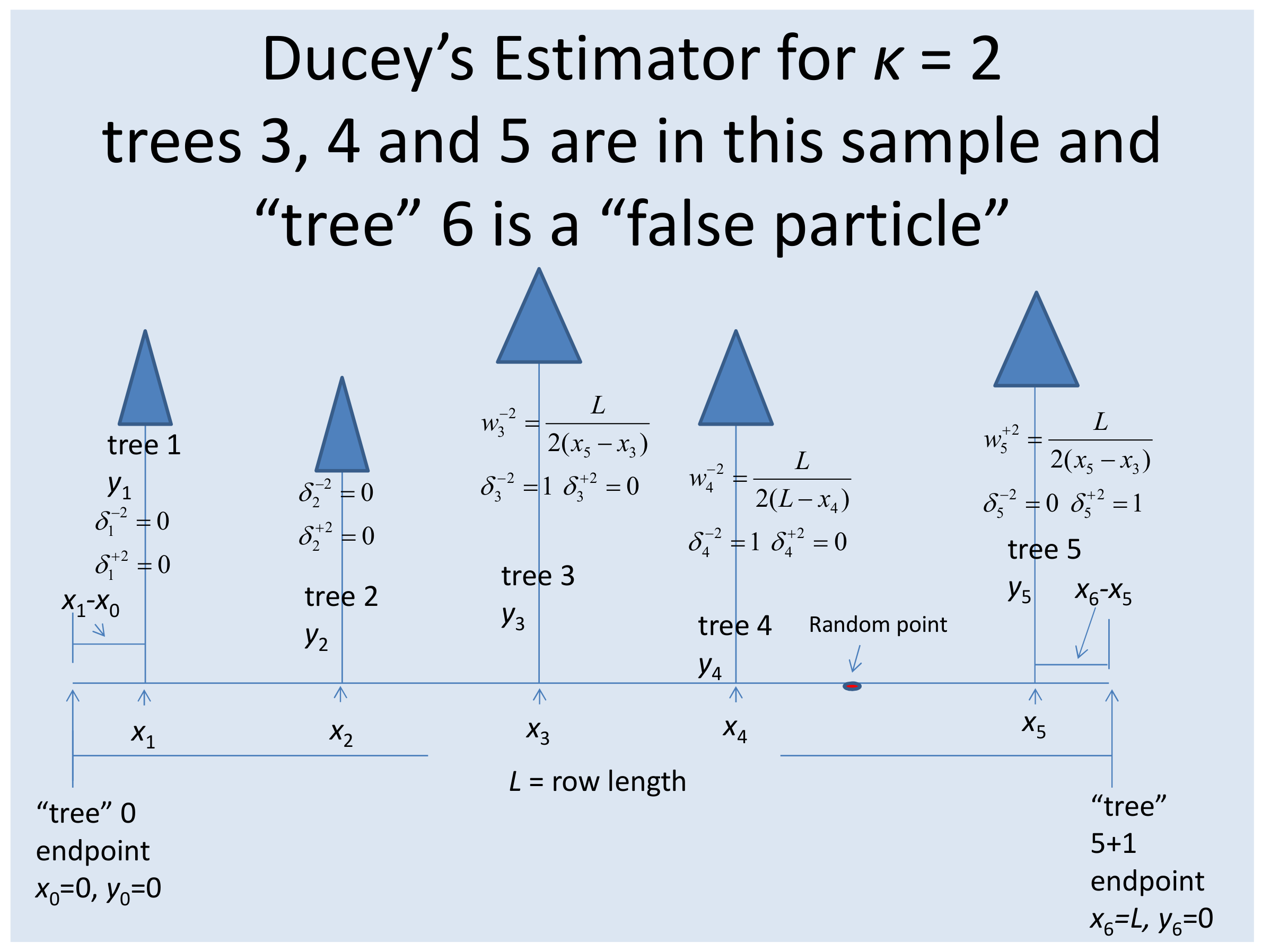
Figure 2 illustrates a more complex example of estimator (1), in which $\kappa$ = 2 so that two trees are selected on either side of the sample gap.

When the randomly located point, z, falls near one of the plantation row endpoints, it is possible that there may not be two trees on either side of the gap into which z falls. This is illustrated in Figure 2, where the second “tree” to the right of the randomly located point z is actually the row end point. In this case, Ducey [1] refers to the sample “tree” as a “false particle”. The attributes of false particles are normally zero. This is shown in Figure 2 by $y_6=0$, because it is the value of an attribute for a “false particle”. For the sample in Figure 2, note that the attribute value for the “false particle” is $y_6=0$, and the location of the “false particle” is $x_6=L$. Thus, Ducey’s estimator becomes:

$${\widehat{Y}}_D=\frac{L\times y_3}{2\left(x_5-x_3\right)}+\frac{L\times y_4}{2\left(L-x_4\right)}+\frac{L\times y_5}{2\left(x_5-x_3\right)}.$$

(6)

Equation (6) only has three additive terms because $y_6=0$ in what would have been the fourth additive term, because “tree” 6 is a “false particle” in this example. If “tree” 6 is not a “false particle”, then Ducey’s estimator (1) with $\kappa =2$ will have four additive terms when evaluated for a particular location of the randomly located point, z.

We sometimes need to consider the mean of $n>1$ independent evaluations of Ducey’s estimator corresponding to n randomly located points $z_i$ on the row populations. This can be expressed as follows:

$${\overline{\widehat{Y}}}_D=\frac{1}{n}\sum _{i=1}^n{\widehat{Y}}_{D,i},$$

(7)

where ${\overline{\widehat{Y}}}_D$ is the mean of n evaluations of Ducey’s estimator corresponding to n randomly located sample points, and ${\widehat{Y}}_{D,i}$ is an evaluation of Ducey’s estimator, Equation (1), associated with a randomly located point, $z_i$. Clearly, Equation (7) is also an unbiased estimator because it is the sum of independent unbiased estimators, and its variance can be easily obtained by standard methods for computing the variance of a linear combination of independent, identically distributed random variables using Equation (4), resulting in

$$var\left({\overline{\widehat{Y}}}_D\right)=\frac{1}{n}var\left({\widehat{Y}}_D\right).$$

(8)

A design-unbiased estimator of the variance (8) where $n\ge 2$ is

$$\widehat{var}\left({\overline{\widehat{Y}}}_D\right)=\frac{1}{n(n-1)}\sum _{i=1}^n{({\widehat{Y}}_{D,i}-{\overline{\widehat{Y}}}_D)}^2,$$

(9)

as indicated by Ducey [1] in Equations (4) and (5). It should be noted that the variance in Equation (8) and the variance estimator (9) are valid for the simple random sampling with replacement scheme developed here, but not for other designs, such as systematic sampling.

2.2. Ratio of Means Estimators

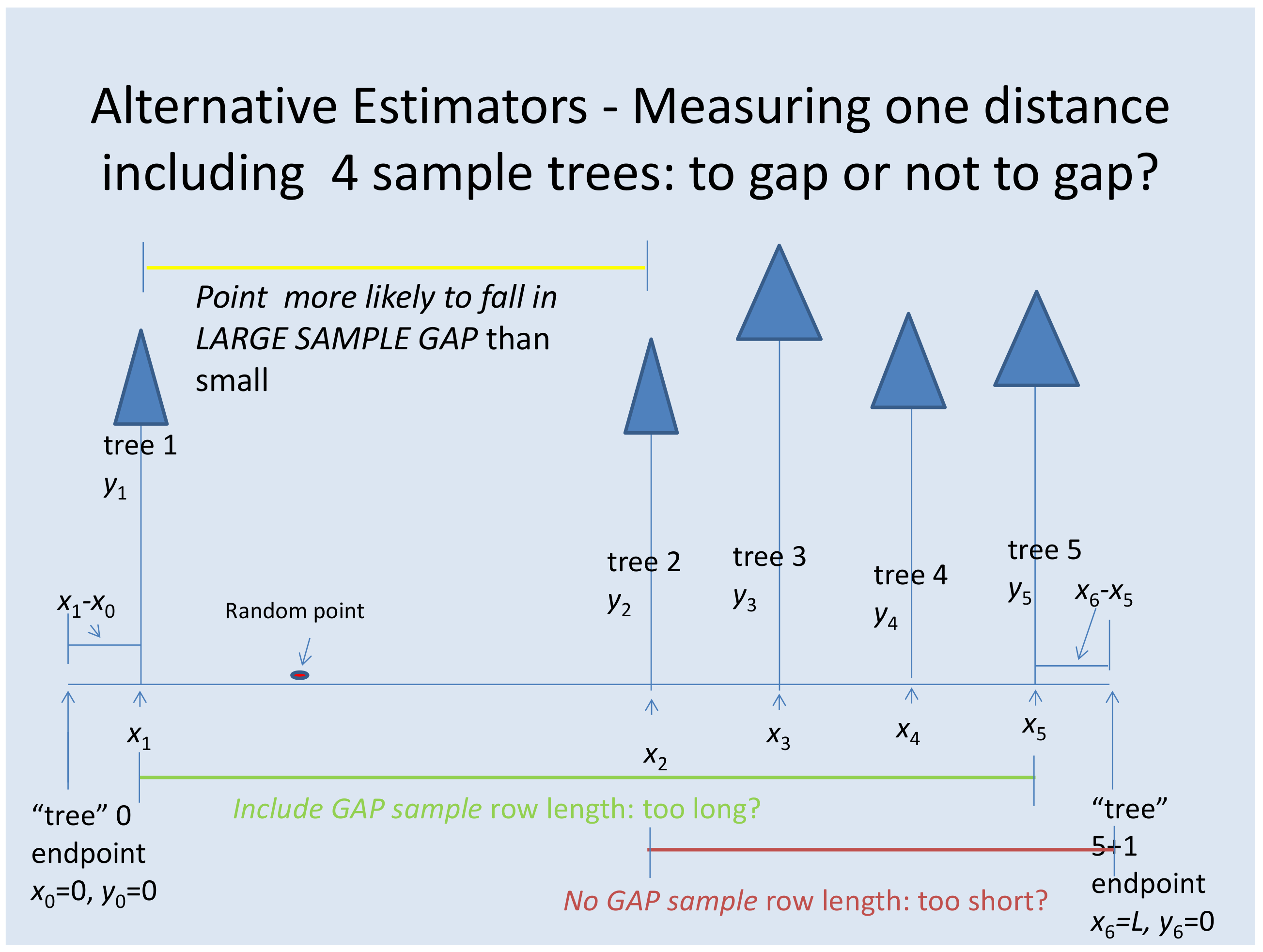
Ratio estimators for plantation row sampling are distinctly different from Ducey’s method because they employ ratios of sums of sample tree attributes, divided by sample row lengths. An important question in formulating these ratio estimators is where to begin the sample row length relative to the location of the random sample point on the population row length, L. Because random sample points are more likely to fall in large gaps between trees on a row, including this gap in the row length may make the sample row length “too large”, meaning that it tends to be larger than average, so that the row length sample segments associated with the sample trees are biased upward. On the other hand, excluding the sample gap in which the random point falls could make the row length sample segments “too small” or biased downwards.

When implementing ratio estimation in the field, a random number, z, is located based on uniform distribution of the interval $\left(0,L\right)$ as with Ducey’s estimator. Point z will fall into a “gap” on the plantation row in between two trees. The main two approaches would be to sample 2$\kappa$ trees including the gap, so that trees on both sides of the sample gap are included in the sample, or to sample 2$\kappa$ trees just following the gap so that the first tree is to the “right” of the gap, and the tree to the left of the gap is not included in the sample. These alternatives are illustrated in Figure 3.

If the sample gap is included, the row measurement will extend from row locations $x_1$ to $x_5$ for sample tree attributes $y_1,y_2,y_3,y_4$. If the sample gap is not included, then the row measurement will be from row locations $x_2$ to $x_6$ for sample tree attributes $y_2,y_3,y_4,y_5$ The “trade-offs” between the two alternative methods of sample row segment selection are illustrated in Figure 3. It is more likely that the randomly located point, z, will fall into a large gap, such as the gap between trees 1 and 2 in Figure 3, than into a small gap. So, it might be that including that gap in the sample row segment will tend to make the sample row segments “too large”. On the other hand, it may be that exclusion of the gap into which z falls could tend to make the sample rows “too short”. Because the choice is not obvious, we evaluate these alternatives using simulated sample row populations. The Ducey [1] estimator, Equation (1), is not subject to this dilemma and has been proven to be design-unbiased.

The ratio of means estimator that includes trees on both sides of the sample gap into which the randomly located point z falls is

$${\widehat{Y}}_{G-RM}=L\frac{\frac{1}{n}{\sum }_{h=1}^n{\sum }_{i=h-1}^{h+2\kappa -1}{y}_i}{\frac{1}{n}{\sum }_{h=1}^n\left(x_{h-1}^{*}-x_{h+2\kappa }^{*}\right)},$$

(10)

where $x_{h-1}^{*}$ is the distance on the row to the position of the tree just to the left of the location of the random sample point, z; $y_i$ is an attribute of tree i; n is the number of sample points, $z_i$, in the sample; $2\kappa$ is a fixed number of sample trees to be used to determine the sample line distance at each sample location; and ${\widehat{Y}}_{G-RM}$ is the mean of ratios estimator for the total of the attribute, y, that includes the sample gap.

The ratio of means estimator that does not include any trees to the left of the sample gap into which the randomly located point z falls is

$${\widehat{Y}}_{NG-RM}=L\frac{\frac{1}{n}{\sum }_{h=1}^n{\sum }_{i=h}^{h+2\kappa }{y}_i}{\frac{1}{n}{\sum }_{h=1}^n\left(x_h^{*}-x_{h+2\kappa +1}^{*}\right)},$$

(11)

where $x_h^{*}$ is the distance on the row to the position of the tree just to the right of the location of the random sample point, z, and ${\widehat{Y}}_{NG-RM}$ is the mean of ratios estimator for the total of attribute y that does not include the sample gap. Borders et al. [4] originally formulated and tested the ratio of means estimator, Equation (10). Ratio estimators have intuitive appeal for the estimation of tree attributes using a fixed number of trees sampled at random locations on plantation rows. The ratio of means approach simply divides the sample mean sum of tree attributes by the sample mean distance occupied by a fixed number of trees at each sample location, z. However, there are technical differences between the ratio of means estimator described here and the classic ratio of means estimator described in Cochran [37] (pp. 150–151) and other standard statistical sampling references. The classical ratio of means estimator [37] (pp. 150–151) is based on sampling two variables, x and y, in each sample unit, where the units are drawn from a population of non-overlapping units comprising a population. So, the application to plantation rows does not exactly correspond to this situation. Also, in the current application to plantation rows, the sample means in the numerator and denominator of the ratio are not known to be unbiased estimators of any population attributes, as would be the case for the ratio of means estimators [37] (pp. 150–151). Therefore, it is not clear that standard statistical results for the ratio of means estimation would apply to the estimators developed for plantation rows. In particular, the ratio of means estimator [37] (pp. 150–151) has a bias of order $1/n$ which tends to be negligible as n becomes large, but this may not be true for the current application to plantation row sampling.

Unfortunately, there is no simple computational expression for the true variances of estimators, (10) or (11). This is the case because the numerator and denominator are both means of n selections of random sample locations, z. Therefore, to approximate the variance of estimators, (10) and (11), for a given sample size, n, we simulated a large number of samples of size n at each given simulated sample row population, as described below.

2.3. Mean of Ratios Estimators

As above, with the ratio of means estimator, the main two possibilities are estimators that include trees on both sides of the sample gap or estimators that include only trees on one side of the sample gap. The mean of ratios estimator that includes trees on both sides of the sample gap into which the randomly located point, z, falls is

$${\widehat{Y}}_{G-MR}=\frac{L}{n}\sum _{h=1}^n{R}_{G-MR,h}=\frac{L}{n}\sum _{h=1}^n\frac{{\sum }_{i=h-1}^{h+2\kappa -1}{y}_i}{x_{h-1}^{*}-x_{h+2\kappa }^{*}},$$

(12)

where $x_{h-1}^{*}$ is the distance on the row to the position of the tree just to the left of the location of the random sample point, z; $y_i$ is an attribute of tree i; n is the number of sample points, $z_i$, in the sample; $2\kappa$ is a fixed number of sample trees to be used to determine the sample line distance at each sample location, $R_{G-MR,i}=\frac{{\sum }_{i=h-1}^{h+2\kappa -1}{y}_i}{x_{h-1}^{*}-x_{h+2\kappa }^{*}}$; and ${\widehat{Y}}_{G-MR}$ is the mean of ratios estimator for the total of attribute y that includes the sample gap.

Because all possible sample gap locations into which the randomly located point, z, may fall can theoretically be enumerated (and in simulated row populations will actually be known) an expression for the true variance of the ratio of means estimator (12) including the sample gap is

$$var\left({\widehat{Y}}_{G-MR}\right)=\frac{L^2}{n}var\left(R_{G-MR,r}\right)=\frac{L}{n}\sum _{r=1}^{N+1}{R}_{G-MR,r}^2\times \left(x_r-x_{r-1}\right)-\frac{L^2}{n}{\left(E\left[R_{G-MR}\right]\right)}^2,$$

(13)

where

$$E\left(R_{G-MR,r}\right)=\frac{1}{L}\sum _{r=1}^{N+1}{R}_{G-MR,r}\times \left(x_r-x_{r-1}\right).$$

(14)

Mean of ratio estimators are not generally unbiased, so it may not be surprising that we cannot prove that $E\left({\widehat{Y}}_{G-MR}\right)$ is necessarily equal to Y. We evaluated the magnitude of the bias in this estimator through simulation studies.

Because the summed terms in estimator (12) are independent and identically distributed, by logic, they are similar to that used for the variance estimation in Ducey’s equation. Thus, the estimate of the variance of the mean of ratios estimator is

$$\widehat{var}\left({\widehat{Y}}_{G-MR}\right)=\frac{L^2}{n(n-1)}\sum _{h=1}^n{(R_{G-MR,h}-{\overline{R}}_{G-MR})}^2,$$

(15)

where

$${\overline{R}}_{G-MR}=\frac{1}{n}\sum _{h=1}^n{R}_{G-MR,h}.$$

(16)

However, because, as has been noted above, the mean of ratios estimator is not unbiased, this variance estimator is not unbiased for the Mean Square Error (MSE) of estimator (12). However, if the estimation bias is small for estimator (12), the bias in the variance estimation in Equation (15) for MSE should be small as well.

The mean of ratios estimator that does not include trees on both sides of the sample gap into which the randomly located point, z falls, but only includes trees in the direction of travel (the “right side” in Figure 3) is

$${\widehat{Y}}_{NG-MR}=\frac{L}{n}\sum _{h=1}^n{R}_{NG-MR,h}=\frac{L}{n}\sum _{h=1}^n\frac{{\sum }_{i=h}^{h+2\kappa }{y}_i}{x_h^{*}-x_{h+2\kappa +1}^{*}},$$

(17)

where ${\widehat{Y}}_{NG-MR}$ is the mean of ratios estimator for the total of attribute y that does not include the sample gap; $x_h^{*}$ is the distance on the row to the position of the tree just to the right of the location of the random sample point, z; and $R_{NG-MR,h}=\frac{{\sum }_{i=h}^{h+2\kappa }{y}_i}{x_h^{*}-x_{h+2\kappa +1}^{*}}$.

As with the variance of estimator (14) above, all possible sample gap locations into which the randomly located point, z, may fall can theoretically be enumerated, leading to the following expression for the true variance of the ratio of means estimator, not including the sample gap (17):

$$var\left({\widehat{Y}}_{NG-MR}\right)=\frac{L^2}{n}var\left(R_{NG-MR,r}\right)=\frac{L}{n}\sum _{r=1}^{N+1}{R}_{NG-MR,r}^2\times \left(x_r-x_{r-1}\right)-\frac{L^2}{n}{\left(E\left[R_{NG-MR,r}\right]\right)}^2,$$

(18)

where

$$E\left(R_{NG-MR,r}\right)=\frac{1}{L}\sum _{r=1}^{N+1}{R}_{NG-MR,r}\left(x_r-x_{r-1}\right).$$

(19)

As was the case for estimator (12), we cannot prove that $E\left({\widehat{Y}}_{NG-MR}\right)$ is necessarily equal to Y. In fact, because the mean of ratios estimator is not consistent, its bias does not decrease with an increase in sample size [38] (pp. 89–90), so often, the ratio of means estimator is preferred. The magnitude of the bias in estimator ${\widehat{Y}}_{NG-MR}$ was evaluated through simulation studies. It is noted that, in most applications of the mean of ratios estimator, the expected values of the variables in the numerators and denominators of the ratios are means of important population attributes. It is not clear that this would be the case for Equations (12) and (17) in the current application.

2.4. Fixed-Length Row Sampling

We also evaluated fixed-length row sampling in which the trees within a fixed row length following the position of the randomly located point, z, were used as sample trees. Using simulations, we adjusted row lengths so that the expected number of trees sampled on each sample row segment would be equal to the number of trees sampled by Ducey’s method (Equation (1)), the ratio of means estimators (Equations (10) and (11)) and the mean of ratios estimators (Equations (12) and (17)). In the simulations described below, the performance of each of these estimators was evaluated for several values of $2\kappa$, the number of trees sampled at each random point location.

2.5. Simulated Plantation Row Sampling

We evaluated the plantation row sampling estimators above using two simulated plantation rows. One population contained a substantial number of gaps between trees on rows that would be typical of the results of thinning and/or mortality. This population will hereafter be referred to as GAPPY. The other population, hereafter referenced as NOT GAPPY, did not contain many large gaps between trees on a row and was representative of populations that may be found in younger plantations prior to thinning and substantial mortality. The NOT GAPPY population included a small amount of “error” in tree spatial locations on rows so that the spacing was not exactly equal and moderately-sized gaps did occur.

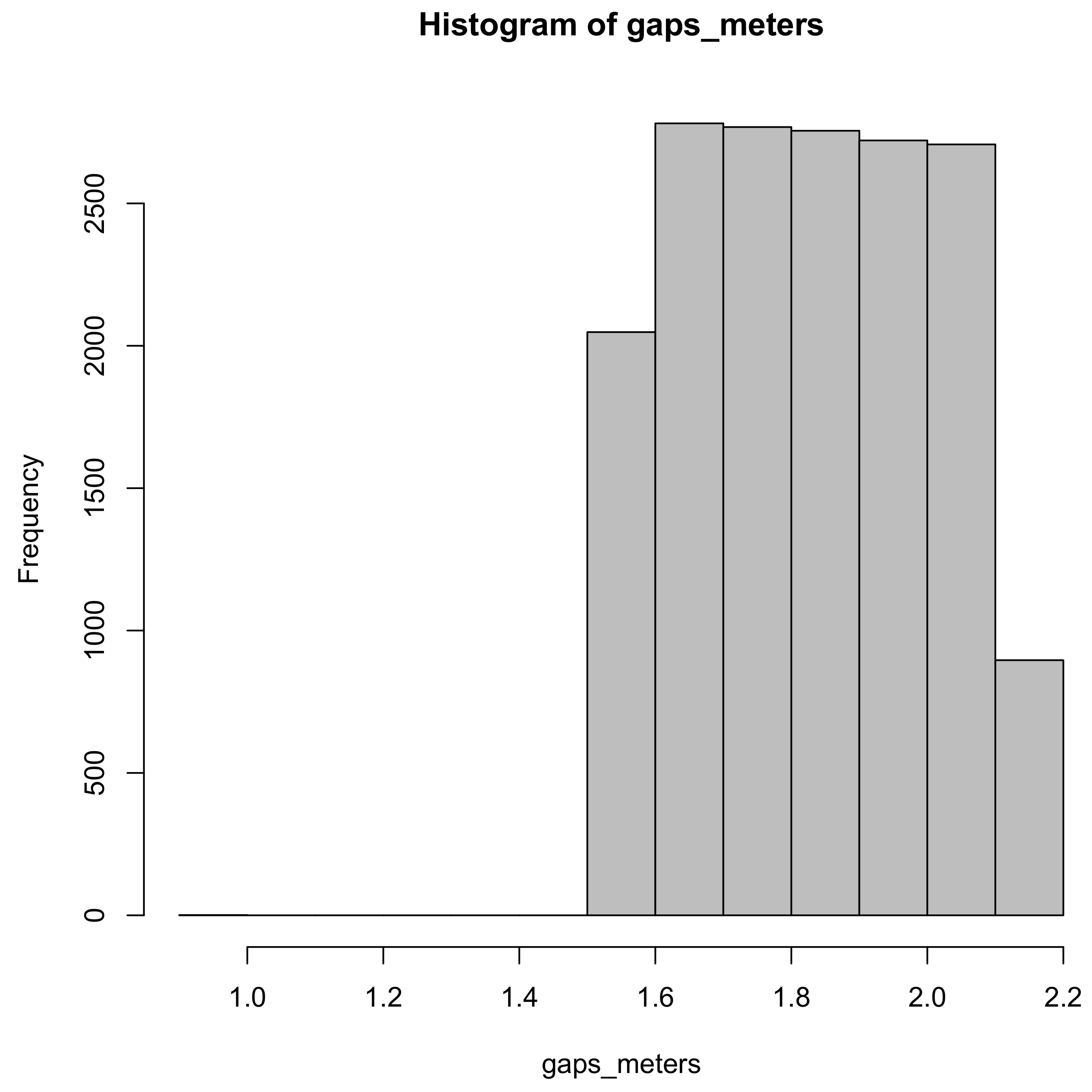
The NOT GAPPY population was constructed with a target row length of 30,408 m, with a mean inter-tree distance of 1.83 m, and a standard deviation of inter-tree distance of 0.18 m. The minimum inter-tree distance was 1.10 m, and the maximum inter-tree distance was 2.13 m. The total number of trees on the NOT GAPPY row was 16,667. A histogram indicating the distribution of inter-tree distances on the NOT GAPPY row is illustrated in Figure 4.

The mid-ranges of this histogram are roughly uniform, with smaller numbers of inter-tree gaps at the large and small classes in the histogram.

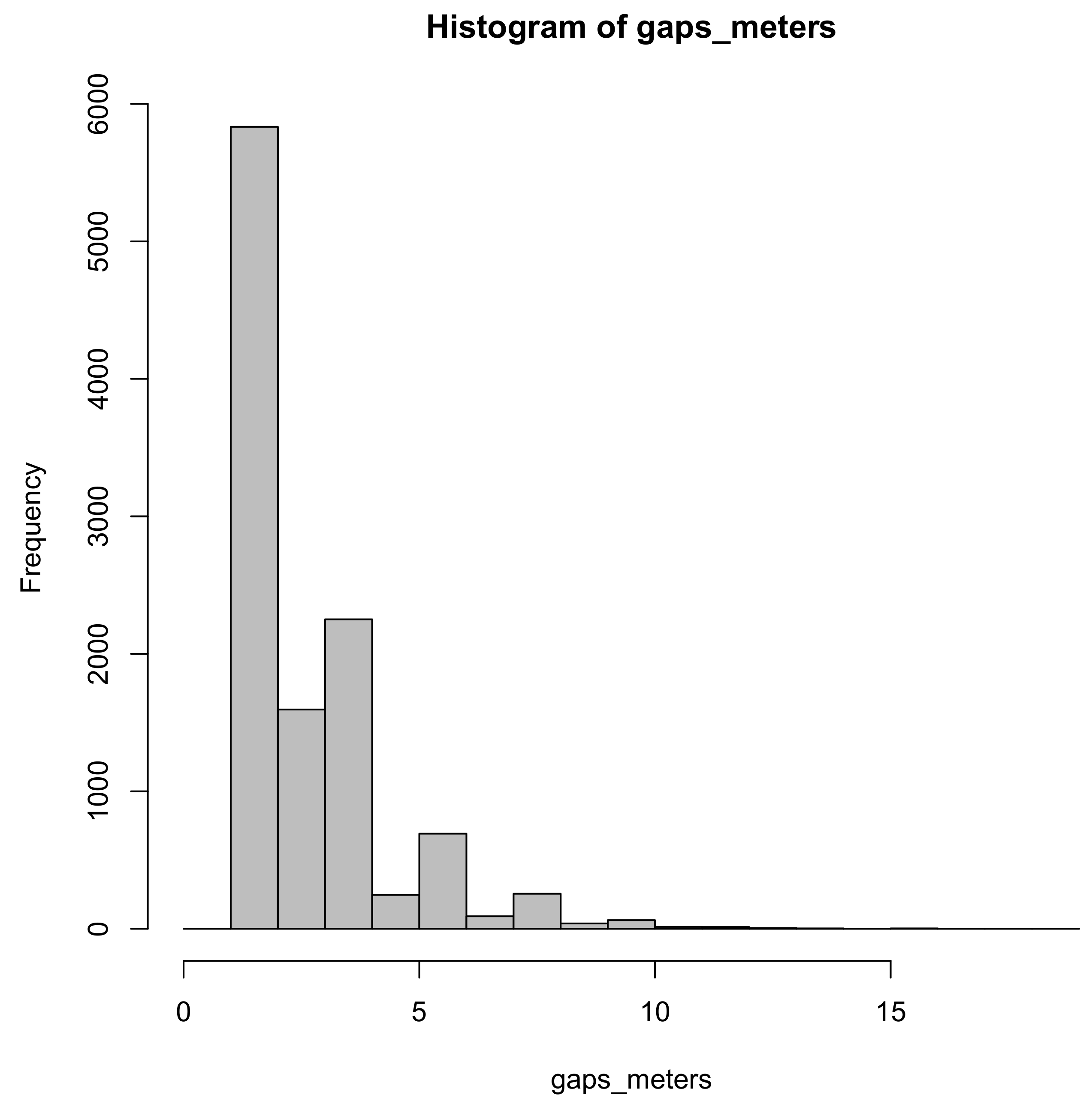
The GAPPY row population also had a target length of 30,408 m. The mean inter-tree distance on the GAPPY row was 2.74 m, with a standard deviation of 2.26 m. The GAPPY row population had a minimum inter-tree distance of 1.10 m and a maximum inter-tree distance of 18.26 m. There were a total of 11,109 trees on the GAPPY population row. The histogram shown in Figure 5 illustrates the distribution of inter-tree gap distances for the GAPPY row.

As might be expected, the histogram is roughly inverse-J shaped with a larger number of small inter-tree gaps and a smaller number of large inter-tree gaps.

Using Ducey’s estimator, Equation (7), and the mean of ratios estimators (Equations (12) and (17)), exact values of bias, variance and mean square error were computed using the variance and expected value formulas indicated above for a sample size of n randomly located points, $z_i$, on the GAPPY and NOT GAPPY simulated row populations. It was not possible to compute exact variances for the ratio of means estimators (Equations (10) and (11)) or for the fixed length row estimator, so a simulation script was written in R [39], and 1 million simulated samples of size $n=10$ were performed on the GAPPY and NOT GAPPY populations in order to closely approximate the true bias and variance associated with the ratio of means estimators. In each case, the estimators were used to estimate the total numbers of trees in the GAPPY and NOT GAPPY simulated row populations, so that the variable $y_i=1$ for all trees included in the sample and $y_i=0$ for $i=0$, and $i=N+1$ at the endpoint locations $x_0=0$ and $x_{N+1}=L$. Simulations were conducted for values of $\kappa$ ranging from 1 to 6 (2 to 12 trees per sample row) on both the GAPPY and NOT GAPPY populations. Simulations for odd tree numbers were not conducted, because Ducey’s method requires even numbers of trees per each sample location. The other methods can accommodate odd numbers of trees per sample row; however, while simulations using the odd tree numbers 3, 5, 7, 9 and 11 trees per sample row were not conducted, it is very likely they would be quite close to results interpolated between adjacent simulations using even tree numbers as will be seen on examination of the simulation results below.

3. Results

3.1. NOT GAPPY Simulation

Figure 6 illustrates the results of the simulation on the NOT GAPPY population row for $n=10$ randomly located sample points, $z_i$, on the NOT GAPPY row.

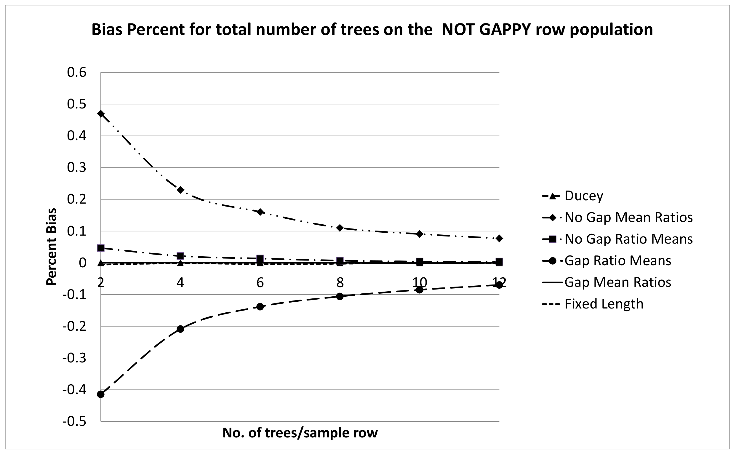
For this population, which does not contain many large gaps, the bias for all of the estimators was less that 0.5 percent in absolute value, even for $\kappa =1$ (two trees per sample row). These biases were computed as the average difference between the estimated total number of trees and the actual total number of trees. Ducey’s estimator, ${\overline{\widehat{Y}}}_D$, shown in Equation (7), is design-unbiased, and therefore, a bias of zero is indicated on Figure 6 for all values of $\kappa$ ranging from 1 to 6 (two to 12 trees per sample row). The fixed-length row estimator is also design-unbiased, although we plotted the extremely small amounts of bias seen in 1 million simulation trials in Figure 6, so that in the figure, the results are not distinguishable from those of Ducey’s estimator. Although none of the ratio estimators are design-unbiased, some of them showed extremely small biases in the simulation trials. In particular, the bias from the mean of ratios estimator, including the gap, ${\widehat{Y}}_{G-MR}$, from Equation (12), was so small for this simulation that it is not distinguishable from zero in Figure 6, and its performance in terms of bias on the NOT GAPPY population was, for all practical purposes, the same as Ducey’s estimator and the fixed-length row estimator which are design-unbiased. The ratio of means estimator that does not include the sample gap, ${\widehat{Y}}_{NG-RM}$, shown in Equation (11) does show a very small amount of bias—less than 0.1 percent for $\kappa =1$ (two trees per sample row) and decreasing to an even smaller and more negligible amount as $\kappa$ increases in Figure 6. The positive bias, ${\widehat{Y}}_{NG-RM}$, shown in Equation (11), though small, is consistent with the idea that excluding the sample gaps (which tend to be larger than typical because the random points are more likely to fall into large gaps) may tend to make the sample row lengths somewhat “too small”. Because the average of the sample row lengths is in the denominator of the estimator, ${\widehat{Y}}_{NG-RM}$, shown in Equation (11), a positive bias is expected if these lengths tend to be somewhat too small.

A bias that was substantially larger in magnitude was indicated for the ratio of means estimator that included the sample gap, ${\widehat{Y}}_{G-RM}$, shown in Equation (10). In this case, the fact that the randomly located point tends to fall in larger gaps tends to make the average sample row length too large in regard to the denominator of (10), which results in underestimation (and recall the biases here are based on the estimated value minus the actual values). Nevertheless, the biases associated with this estimator are smaller than 0.5 percent in absolute value, even for $\kappa =1$ (two trees per sample row) and decline to even more negligible values as $\kappa$ increases, becoming near or less than 0.1 percent for $\kappa \ge 4$ (more than or equal to eight trees per sample row).

The trends in bias for the mean of ratios estimator not including the sample gap, ${\widehat{Y}}_{NG-MR}$, shown in Equation (17), indicate a positive bias, ranging from just less that 0.5 percent for two trees per sample row ,to near or less than 0.1 percent for eight or more trees per sample row. The biases for ${\widehat{Y}}_{NG-MR}$ and ${\widehat{Y}}_{NG-RM}$ are similar in absolute value, but opposite in sign for the number of trees per sample row, ranging from two to 12, and decline substantially as the number of trees per sample row increases. These two estimators, ${\widehat{Y}}_{NG-MR}$ and ${\widehat{Y}}_{NG-RM}$, show the greatest magnitudes of bias among the estimators tested. However, in the NOT GAPPY population row, even these estimators show amounts of bias that are probably negligible, especially since it is very likely that practical applications of plantation row sampling would sample at least four trees per sample row and more likely six to 10. When six trees per row segment are sampled, the magnitudes of bias in these two methods drops to about a third of the biases associated with sampling two trees per sample row segment.

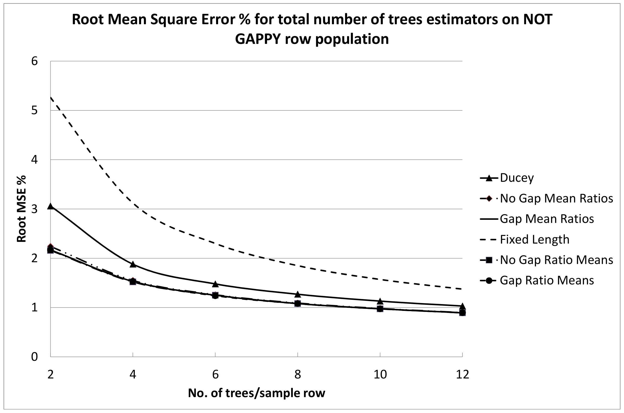
The Root Mean Square Error percentages (RMSE%) for each of the estimators tested on the NOT GAPPY row are illustrated in Figure 7 for two to 12 trees per sample row. When evaluating RMSE performance, it should be recalled that MSE = ((Bias)${}^2$ + Variance), and RMSE is the square root of the MSE. Thus, for methods that show large biases on the GAPPY plantation row especially, this contributes substantially to increased RMSE compared to methods that are unbiased or have small biases.

All of the estimators that sample fixed numbers of trees per random sample location were superior to fixed-length row segment sampling in terms of RMSE%. Ducey’s estimator, ${\overline{\widehat{Y}}}_D$, shown in Equation (7), showed RMSE% values that were only slightly higher than the other methods, and they were especially close when six trees or more weare sampled per sample row segment, so that the difference between them shown in this simulated row population is negligible for practical purposes. The performances of the ratio estimators, ${\widehat{Y}}_{NG-MR}$, shown in Equation (17), ${\widehat{Y}}_{G-MR}$, shown in Equation (12), ${\widehat{Y}}_{NG-RM}$, shown in Equation (11), and ${\widehat{Y}}_{G-RM}$, shown in Equation (10) are so similar in Figure 7 for two to 12 trees per sample row segment that they are virtually indistinguishable. Inspection of Figure 7 indicates that for most of these estimators, the RMSE% with six trees per sample row segment was nearly half of the RMSE% for two trees per row segment. As the number of trees per sample row segment increased from eight to 12, there was very little decrease in RMSE%. This suggests that sampling with six to eight trees per sample row segment for plantation row populations is preferable . The low values of RMSE% in Figure 7 are indicative of the fact that it is comparatively easy to estimate the total tree number if the row length is known and gaps between trees are fairly consistent. Indeed if there was absolutely no variation in gap widths, knowing the gap width and row length would be sufficient to estimate the total tree number exactly.

3.2. GAPPY Simulation

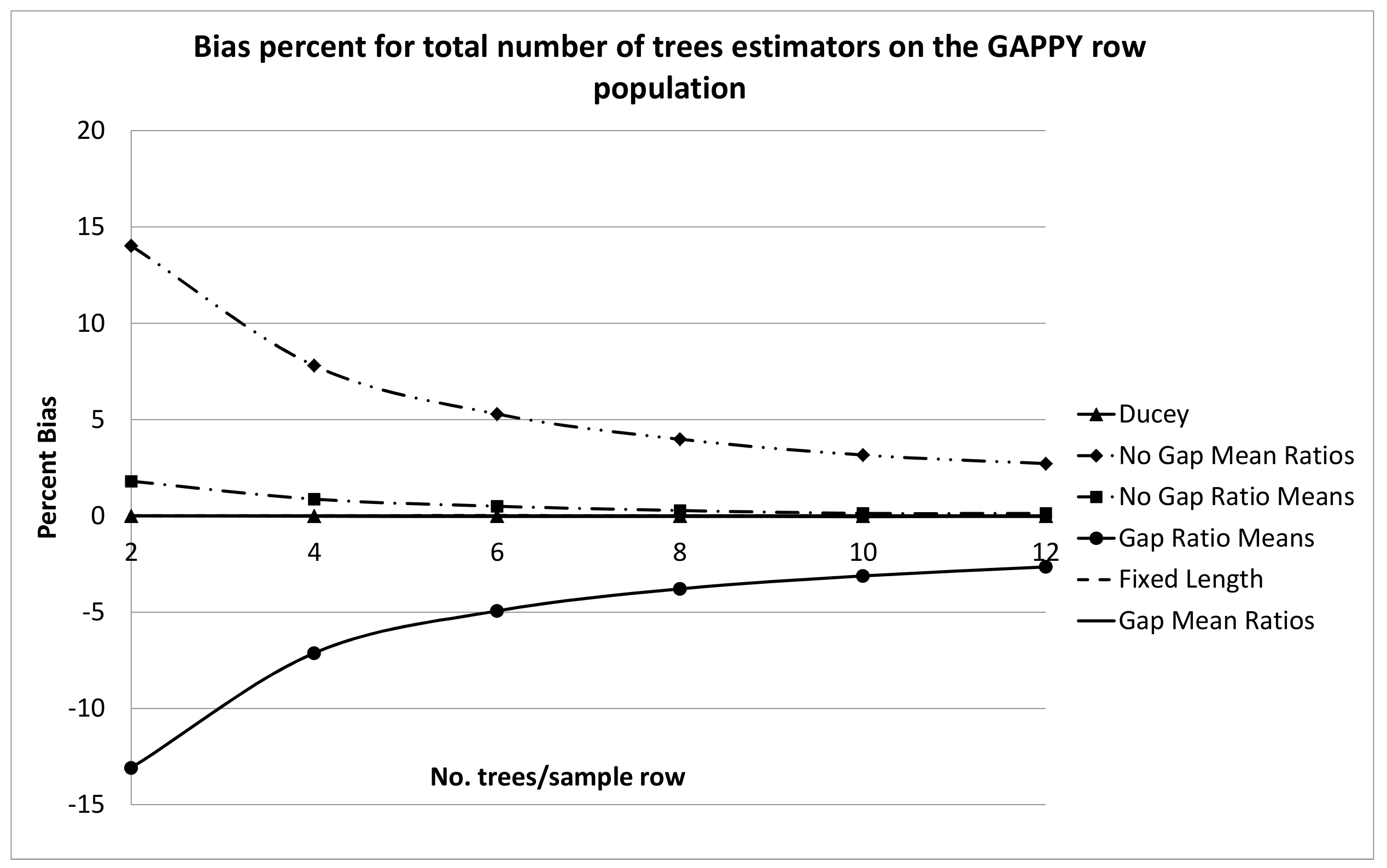
The bias percentages for the GAPPY simulated row population are illustrated in Figure 8.

As in Figure 6, there was no bias in Ducey’s estimator, ${\overline{\widehat{Y}}}_D$ (Equation (7)), and the biases in the fixed row length estimator and the mean of ratios estimator, including the sample gap, ${\widehat{Y}}_{G-MR}$, (Equation (12)) were so small that they cannot be distinguished from zero in Figure 8. As indicated above, the fixed row length estimator and Ducey’s estimator are design-unbiased. Very small biases due to simulation are too small to discern visually in Figure 8 for the fixed-row length estimator, whose performance was evaluated based on 1 million simulation trials. Bias percentages associated with the ratio of means estimator, not including the sample gap, ${\widehat{Y}}_{NG-RM}$ (Equation (11)), are visible in Figure 8, but are negligible for practical purposes and very close to nil for six or more sample trees per sample row segment. However, substantial biases are evident for the GAPPY population with the ratio of means estimator that includes the sample gap, ${\widehat{Y}}_{G-RM}$ (Equation (10)), and the mean of ratios estimator that does not include the sample gap, ${\widehat{Y}}_{NG-MR}$ (Equation (17)), especially for eight or fewer trees per sample row, where biases ranged from about 4 percent to 14 percent for two trees per sample row. Once again, the ratio of means estimator including the sample gap, ${\widehat{Y}}_{G-RM}$ (Equation (10)) showed a negative bias (based on estimated minus actual tree numbers), possibly because the average sample row length in the denominator of the estimator was “too large”, as random sample points, z, were more likely to fall in large gaps. The performance of the mean of ratios estimator not including the sample gap, ${\widehat{Y}}_{NG-MR}$ (Equation (17)) showed a positive bias which was nearly a “mirror image” of ${\widehat{Y}}_{NG-RM}$, ranging from about 14 percent for two trees per sample row segment to around 3 percent with 12 trees per sample row segment.

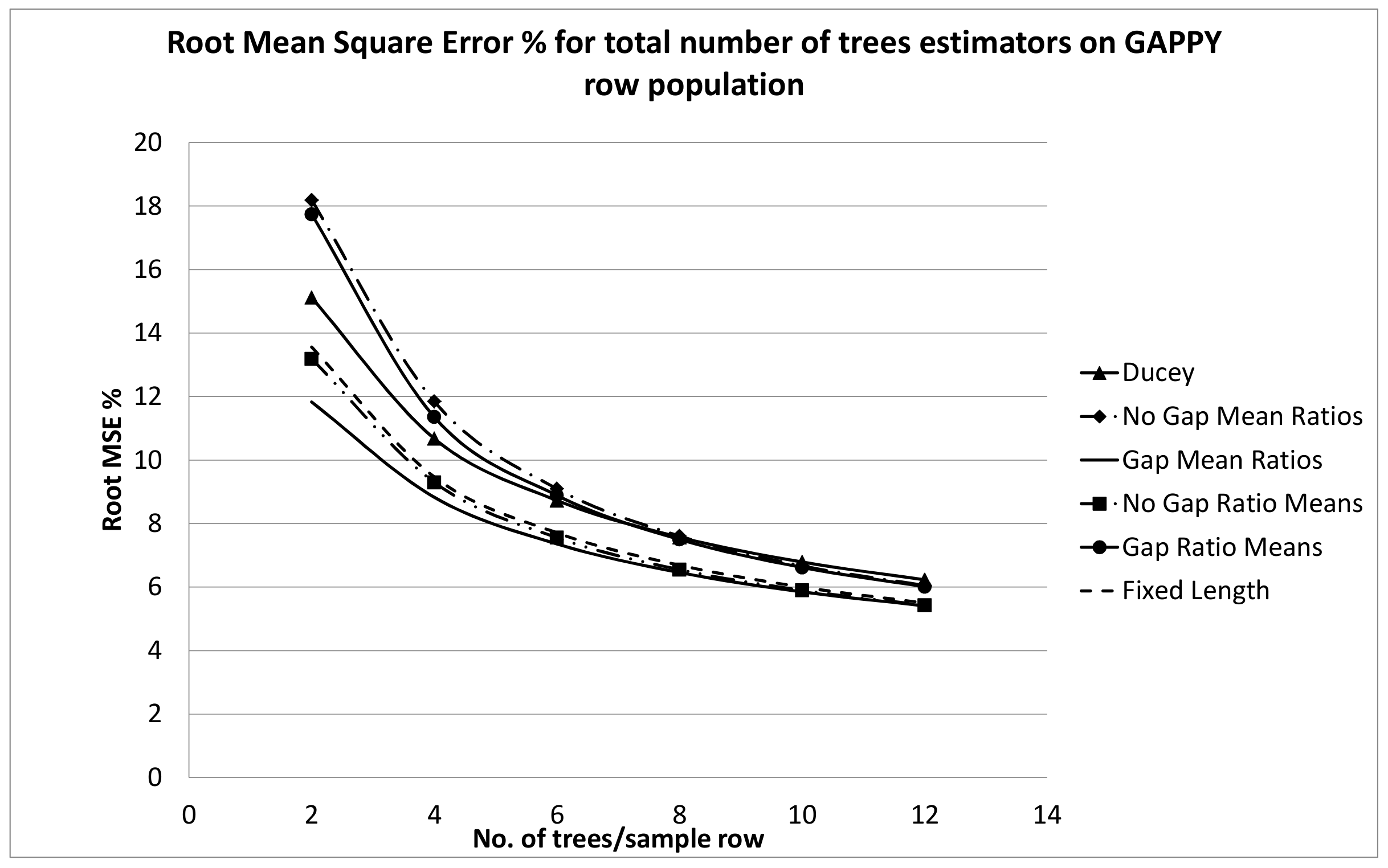
The levels of RMSE% indicated for the GAPPY simulated row population in Figure 9 were substantially higher than for the NOT GAPPY population, indicating the greater difficulty in estimation on sample rows that contain large gaps, possibly due to thinning and/or mortality mixed with much smaller gaps associated with the original spacing at the time of planting.

This resulted in a much more diverse row population than the NOT GAPPY population. The best RMSE% performance was associated with the mean of ratios estimator, including the sample gap ${\widehat{Y}}_{G-MR}$ (Equation (12)). However the fixed length sample row and the ratio of means not including the sample gap, ${\widehat{Y}}_{NG-RM}$ (Equation (11)) were quite close especially for six or more trees per sample row segment. Ducey’s estimator, ${\widehat{Y}}_{NG-RM}$ (Equation (11)) had a somewhat higher RMSE% than the latter two estimators, but the difference is probably not practically significant. The highest RMSE% values were associated with the mean of ratios not including the sample gap, ${\widehat{Y}}_{NG-MR}$ (Equation (17)), and the ratio of means, including the sample gap, ${\widehat{Y}}_{G-RM}$ (Equation (10)). This could be partially due to the fact that they also had the highest levels of bias in Figure 8, and bias is included in the calculation of RMSE% . For situations with six or more trees per sample row segment, the RMSE% values for these latter two estimators became very close to that of Ducey’s method and fairly close to the methods with the lowest RMSE% values. As expected, all methods showed trends of decreasing a RMSE% with an increasing number of trees per sample row segment, so that the RMSE% with 12 trees per sample row segment converged to around 6 percent for all methods, which is a half to a third of the RMSE% values associated with two trees per sample row segment, depending on the estimation method.

4. Discussion

There was very little practical difference between the row sampling estimators tested on the NOT GAPPY row population. This is probably due to the substantially lower variation in gap sizes compared to the GAPPY population. Practically significant differences between the methods emerged in the simulations on the GAPPY row population. There is probably no good reason to use the ratio of means estimator including the sample gap, ${\widehat{Y}}_{G-RM}$ (Equation (10)) or the mean of ratios estimator not including the gap, ${\widehat{Y}}_{NG-MR}$ (Equation (17)) due to the possibility of substantial bias, as illustrated in Figure 8 for the GAPPY row population, and the fact that it is no easier to collect data for the latter two estimators than for alternative estimators that show zero or negligible bias on both the GAPPY and NOT GAPPY row populations.

The ratio of means estimator not including the sample gap, ${\widehat{Y}}_{NG-RM}$, performed well on both the GAPPY and NOT GAPPY row populations. It displayed somewhat more bias in the GAPPY simulation for lower numbers of trees per sample row segment than ${\widehat{Y}}_{G-MR}$ (Equation (12)), Ducey’s estimator, ${\overline{\widehat{Y}}}_D$ (Equation (7)), or the fixed-length sample row, but that bias would not be practically significant especially when six or more trees per random sample location are used. This ratio estimator was the estimator first proposed by Borders et al. [4]. It should be recalled (as indicated above where the ratio of means estimators were introduced) that the ratio of means estimators presented in this article differ from the classical ratio of means estimators discussed in standard sampling references, such as Cochran [37] (pp. 150–151). Therefore, it is not clear that theorems which show that ratio of means estimators can be consistently applied to the estimators used here. This is one reason why we evaluated these estimators using simulations.

The superior performance of the mean of ratios estimator, including the sample gap, ${\widehat{Y}}_{G-MR}$ (Equation (12)), is likely to be due to the fact that the randomly located point, z, falls into a gap with probability proportional to its size. Because the sample gap is part of the sample row length, this makes ${\widehat{Y}}_{G-MR}$ roughly similar to an inverse probability estimator, as the denominators of the ratios become roughly (but not exactly) proportional to the probability that that particular row segment is selected as a sample segment. Schreuder et al. [38] (p. 90) pointed out that if the denominators of the ratios for the mean of ratios estimator are proportional to the probability of sample selection, then the mean of ratios estimator is unbiased. However, the ${\widehat{Y}}_{G-MR}$ estimator is not mathematically unbiased because the proportion is not exact. Nevertheless, this latter estimator showed extremely small biases in simulations on the GAPPY and NOT GAPPY row populations, which were practically negligible.

For the mean of ratios estimator that does not include the sample gap, ${\widehat{Y}}_{NG-MR}$ (Equation (17)) the similarity to an inverse probability estimator was completely lost, resulting in poor bias performance on the GAPPY row population. As indicated above, the ratio of means estimator that does not include the sample gap, ${\widehat{Y}}_{NG-RM}$ (Equation (11)) is probably superior to ${\widehat{Y}}_{G-RM}$ (Equation (10)) because the mean row length in the latter estimator tends to be too large, since the random point, z, tends to select larger sample gaps. Because of their algebraic formulation, the ratio of means estimators cannot be formulated to be similar to inverse probability estimators. The inclusion of the sample gap was beneficial to the mean of ratios estimator (decreased bias), but detrimental to the ratio of means estimator (increased bias).

The fixed length plot sample performed well, although it clearly had a higher RMSE% for the NOT GAPPY population than for the other row sampling estimators. This may be due to the fact that the number of trees per fixed length row can still vary due to random starting points while the number of trees per sample location is, of course, the same for the fixed number of trees estimators, and in the NOT GAPPY simulation there is less variation in sample segment length for these estimators. For the GAPPY simulation, much of the RMSE% advantage of the fixed number of trees estimators was lost, because in this population, there was much more variation in sample segment row lengths for these estimators. There are practical advantages to the estimators that use a fixed number of trees per plot. To be design-unbiased, the beginning point for the fixed-length row estimator is assumed be assigned randomly along the plantation row length. This means the beginning point should be located where it falls within the gap between the two trees where it is located. This may be difficult to actually do in the field, and crews may tend to gravitate to a consistent location within sample gaps, such as the middle of the gap or either end of the gap. With Ducey’s method and the ratio estimators tested here which select a fixed number of trees associated with each randomly located point, z, it is only necessary for crews to locate the gap into which the random point falls, because the location of the sample point within the gap does not affect the fixed number of trees per sample segment estimators.

In particular, when six or more trees per sample row segment were used, Ducey’s estimator, ${\overline{\widehat{Y}}}_D$ (Equation (7)) performed quite well, with an RMSE% that was not substantially worse than the best RMSE% performers. Ducey’s method is design-unbiased so it will be mathematically guaranteed to be unbiased for any sample row population. Although we tried to select two populations that would span a wide range of likely possibilities for gap distributions on plantation rows, it was impossible to test every possible gap distribution by simulation methods. Considering this fact, Ducey’s estimator becomes quite attractive.

In the field, it will be necessary to measure the location of each tree in the sample row segment if Ducey’s estimator, ${\overline{\widehat{Y}}}_D$ (Equation (7)) is used. In particular, for sample row segments with smaller fixed numbers of trees, such as 4 to 6, a tape could be stretched along the row between the trees on the ends of the row segment, and the position of each tree recorded, along with measurements of tree attributes, such as dbh and height, that may be desired. This information could be used to accomplish estimation with Ducey’s method in a software routine.

The RMSE% results in Figure 7 and Figure 9 tended to indicate that six to eight trees per sample segment should probably be sampled, because this provides a definite gain in RMSE% compared to sampling four or fewer trees. For the NOT GAPPY population especially, there seems to be little advantage to sampling more than eight trees per sample row segment, but RMSE% is substantially reduced by sampling at least six trees per sample row segment. This is fairly similar to guidelines that are often given for selection of the number of trees per point when choosing an angle gauge for horizontal point sampling. Iles [40] (p. 526) stated that the best balances of cost for point sampling happen with an average of 4–8 trees per point.

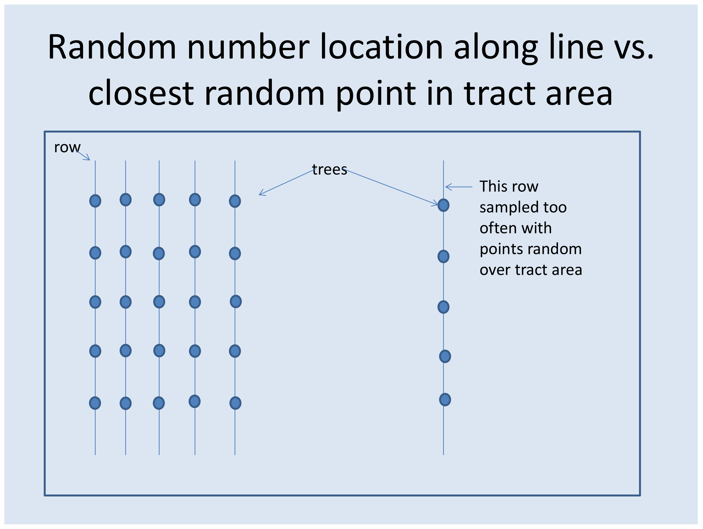
Figure 10 illustrates why it is important in plantation row sampling that the randomly located point, z, is placed with uniform probability over the plantation row length, L, rather than with uniform probability over a two-dimensional land area.

Clearly, if the point is distributed randomly over a two dimensional land area, and then the “closest gap” in plantation rows is selected, the isolated plantation row segment on the right side of Figure 10 will be sampled more intensely than the remainder of the plantation row population. Although Figure 10 is an extreme example, row removal thinning (removing all the trees in selected rows, such as every third row) is very common in plantations in Southeastern USA, and if the randomly-located sample point, z, was distributed over a 2-dimensional land area, next to rows removed by thinning, it would be sampled more intensely than “interior rows” not adjacent to rows removed by thinning. This could have important consequences as it might be expected that trees on rows adjacent to removed rows may experience more diameter growth in years subsequent to thinning than “interior rows” that are not adjacent to removal rows.

In field applications, one will find the value of a random distance, z, with uniform probability for the interval $\left(0,L\right)$, where L is the total row length. We envision that a plantation population can be treated as one long row of length L by joining the ends of adjacent rows in the field. Then, the two dimensional location (e.g., latitude and longitude) of this row distance would need to be determined, most likely in a GIS environment. Field crews would then use a GPS receiver to locate the sample point in the field. Because of possible error in the GPS location, the GPS field location may not always fall exactly on a row. In this case, we recommend choosing the gap between trees that has the closest perpendicular distance to the sample GPS coordinate in the field. A random-start, systematic sampling procedure would be also be possible with field crews locating sample gaps at fixed intervals along plantation rows; however, this would require the total plantation row length to be traversed.

It is important to recognize that accurate estimation of the total row length, L, is vital for the accuracy of the row sampling estimators presented here. Let us formulate a general row sampling estimator as a product of an estimator per unit of row length multiplied by row length:

$$\widehat{Y}=\widehat{L}\times {\widehat{Y}}_{unit/L},$$

(20)

where $Y_{unit/L}$ is the row sampling estimator per unit of L using any of the row sampling estimators above. This could be obtained by setting $L=1$ in any of the estimators above, and $\widehat{L}$ is the estimated row length with $E(\widehat{L})=L$.

Clearly any substantial underestimation or overestimation of L will have a major impact on the estimator, just as errors in the estimation of the total land area can have a large impact on more traditional estimators of forest volume and other attributes. It may be more difficult to accurately identify rows in very old plantations. Merging of multiple rows into one row may cause confusion. There is likely to be some error in the remote sensing technology used to estimate row lengths. It is likely that we can consider row length estimates, $\widehat{L}$, to be scholastically independent of ${\widehat{Y}}_{unit/L}$, because they are estimated by different procedures. In that case, we can apply the formula of Goodman [41] to compute the variance of a product of independent random variables:

$$var\left(\widehat{L}\times {\widehat{Y}}_{unit/L}\right)={\left(E\left[\widehat{L}\right]\right)}^{2}var\left({\widehat{Y}}_{unit/L}\right)+{\left(E\left[{\widehat{Y}}_{unit/L}\right]\right)}^{2}var(\widehat{L})+var\left({\widehat{Y}}_{unit/L}\right)var\left(\widehat{L}\right).$$

(21)

If $var(L)=0$, then Equation (18) trivially reduces to

$$var\left(L\times {\widehat{Y}}_{unit/L}\right)=L^{2}var\left({\widehat{Y}}_{unit/L}\right).$$

(22)

According to Equation (5) in [41], an unbiased estimate of the variance given by Equation (21) is

$$\widehat{var}\left(\widehat{L}\times {\widehat{Y}}_{unit/L}\right)={\left(\widehat{L}\right)}^2\widehat{var}\left({\widehat{Y}}_{unit/L}\right)+{\left({\widehat{Y}}_{unit/L}\right)}^2\widehat{var}(\widehat{L})-\widehat{var}\left({\widehat{Y}}_{unit/L}\right)\widehat{var}\left(\widehat{L}\right),$$

(23)

where $\widehat{var}(\widehat{L})$ is an unbiased estimate of $var(\widehat{L})$, $\widehat{var}({\widehat{Y}}_{unit/L})$ is an unbiased estimate of $var({\widehat{Y}}_{unit/L})$, $\widehat{L}$ is an unbiased estimate of L, and ${\widehat{Y}}_{unit/L}$ is an unbiased estimate of $Y_{unit/L}$. It should be noted that according to [41], the sign on the final term in Equation (23) is negative, rather than the positive sign used for the final term in (21). If unbiased estimators for L and $var(\widehat{L})$ are available, Ducey’s estimator (1) and its associated variance estimator (8) would fit these requirements.

The fact that Ducey’s estimator has a simple variance estimator that is unbiased for its true variance is a major advantage for Ducey’s method. As indicated above, the ratio estimators tested here do not exactly fit the paradigm for ratio estimators developed in standard sampling texts, such as [37], so it is not clear how well approximations traditionally used to estimate the variances of the ratio of means estimators will work in the plantation row sampling application. However, as indicated above, we did present a variance estimator for the mean of ratios estimator including the sample gap, which should work well if the estimation bias is small as it was in our simulations. It may be that bootstrap methods could be employed to estimate variance in the ratio of means estimator if closed-form approximation formulas do not work well. However, we did not test variance estimation methods for the ratio of means estimators in this study.

When the measurement or estimation of row length, L, is problematic, a possible solution is to develop row plots by measuring the distance between the middle of the spaces between rows on either side of the sample row segment, $w_h$, and using this to form a rectangular plot. This may permit one to use the tract area, $\mathcal{A}$, to expand the estimate to tract level. As an example, consider the following adjustment to the Borders et al. (2012) ratio of means estimator (11):

$${\widehat{Y}}_{NG-RM}=\mathcal{A}\frac{\frac{1}{n}{\sum }_{h=1}^n{\sum }_{i=h}^{h+2\kappa }{y}_i}{\frac{1}{n}{\sum }_{h=1}^n{w}_h\left(x_h^{*}-x_{h+2\kappa +1}^{*}\right)}.$$

(24)

This formulation permits the expansion of the sample using the tract area, $\mathcal{A}$, which is generally known even when the total plantation row length may be difficult to measure or estimate. Similar adjustments could be made to the other row sampling estimators presented above.

5. Conclusions

In comparisons among plantation row sampling estimators that select a fixed number of trees per sample row segment using GAPPY and NOT GAPPY simulated row populations, a mean of ratios estimator including the sample gap, ${\widehat{Y}}_{G-MR}$ (Equation 12) and a ratio of means estimator that does not include the sample gap, ${\widehat{Y}}_{NG-RM}$ (Equation (11)) had the best performances in terms of RMSE%. The mean of ratios estimator, ${\widehat{Y}}_{G-MR}$, indicated less bias than ${\widehat{Y}}_{NG-RM}$, although the bias was practically negligible for both estimators.

Ducey’s estimator, ${\overline{\widehat{Y}}}_D$ (Equation (7)) had a slightly higher RMSE% than the latter two ratio estimators but is design-unbiased, so unlike the ratio estimators, Ducey’s estimator is guaranteed to be unbiased for any spatial distribution of trees along plantation rows. This is a substantial advantage because it is impossible to test every possible plantation row’s spatial distribution using simulation methods, and older plantations can display considerable variability in the distribution of gaps between trees on plantation rows due to thinning operations and mortality. Compared with point or plot sampling, these novel row sampling estimators eliminate the need for the problematic location of plot centers and sample points in a tree population with a highly structured spatial distribution. When the best of these row sampling estimators are combined with plantation row lengths measured by remote sensing methods, plantation row sampling may present a viable alternative to more traditional forest sampling techniques, such as point sampling or fixed-radius plot sampling, for forest plantation populations.

References

- Ducey, M.J. Design-unbiased point-to-particle sampling on lines, with applications to areal sampling. Eur. J. For. Res. 2018, 1–17. [Google Scholar] [CrossRef]
- Ducey, M.J. Simple, Design-Unbiased Areal Sampling with Nearest Neighbor Methods. Presented at the 2012 Northeast Mensurationists Meeting, Pennsylvannia State University, State College, PA, USA, 1–2 October 2012. Unpublished Report. [Google Scholar]
- Gregoire, T.G. Design-based and model-based inference in survey sampling: Appreciating the difference. Can. J. For. Res. 1998, 28, 1429–1447. [Google Scholar] [CrossRef]
- Borders, B.E.; Shriver, B.; Cass, R. Row sampling in planted stands. Presented at the 2012 Southern Mensurationists Meeting, Jacksonville, FL, USA, 7–9 October 2012. Unpublished Report. [Google Scholar]
- Eberhart, L.L. Some developments in ‘distance sampling’. Biometrics 1967, 23, 207–216. [Google Scholar] [CrossRef]
- Moore, P.G. Spacing in plant populations. Ecology 1954, 35, 222–227. [Google Scholar] [CrossRef]
- Thompson, H.R. Distribution of distance to the nth neighbor in a population of randomly distributed individuals. Ecology 1956, 37, 391–394. [Google Scholar] [CrossRef]
- Cottam, G. A point method for making rapid surveys of woodlands. Bull. Ecol. Soc. Am. 1947, 28, 60. [Google Scholar]
- Cottam, G.; Curtis, J.T. The use of distance measures in phytosociological sampling. Ecology 1956, 37, 451–460. [Google Scholar] [CrossRef]
- Pollard, J.H. On distance estimators of density in randomly distributed forests. Biometrics 1971, 27, 991–1002. [Google Scholar] [CrossRef]
- Lessard, V.; Reed, D.D.; Monkevich, N. Comparing n-tree distance sampling with point and plot sampling in northern Michigan forest types. North. J. Appl. For. 1994, 11, 12–16. [Google Scholar]
- Jonsson, B.; Holm, S.; Kallur, H. A forest inventory method based on density-adapted circular plot size. Scand. J. For. Res. 1992, 7, 405–421. [Google Scholar] [CrossRef]
- Lynch, T.B.; Rusydi, R. Distance sampling for forest inventory in Indonesian teak plantations. For. Ecol. Manag. 1999, 1999, 215–221. [Google Scholar] [CrossRef]
- Prodan, M. Punkstichprobe für die forsteinrichtung. Forst und Holzwirt 1968, 23, 225–226. (In Germany) [Google Scholar]
- Schreuder, H.T. Sampling Using a Fixed Number of Trees Per Plot; Research Note RMRS-RN-17; USDA Forest Service Southern Rocky Mountain Experiment Station: Fort Collins, CO, USA, 2004.
- Kleinn, C.; Vilčko, F. A new empirical approach for estimation in k-tree sampling. For. Ecol. Manag. 2006, 237, 522–533. [Google Scholar] [CrossRef]
- Haxtema, A.Z.; Temesgen, H.; Marquardt, T. Evaluation of n-tree distance sampling for inventory of headwater riparian forests of western Oregon. West. J. Appl. For. 2012, 27, 109–117. [Google Scholar] [CrossRef]
- Magnussen, S.; Kleinn, C.; Picard, N. Two new density estimators for distance sampling. Eur. J. For. Res. 2008, 127, 213–224. [Google Scholar] [CrossRef]
- Magnussen, S.; Fehrmann, L.; Platt, W.J. An adaptive composite density estimator for k-tree sampling. Eur. J. For. Res. 2012, 131, 307–320. [Google Scholar] [CrossRef]
- Magnussen, S. A new composite k-tree estimator of stem density. Eur. J. For. Res. 2012, 131, 1513–1527. [Google Scholar] [CrossRef]
- Horvitz, D.G.; Thompson, D.J. A generalization of sampling without replacement from a finite universe. J. Am. Stat. Assoc. 1952, 47, 663–685. [Google Scholar] [CrossRef]
- Delincé, J. Robust density estimation through distance measurements. Ecology 1986, 67, 1576–1581. [Google Scholar] [CrossRef]
- Overton, W.S.; Stehman, S.V. The Horvitz-Thompson theorem as a unifying principle for probability sampling: With examples from natural resource sampling. Am. Stat. 1996, 49, 261–268. [Google Scholar]
- Barabesi, L.; Fattorini, L. The use of replicated plot, line, and point sampling for estimating species abundance and ecological diversity. Environ. Ecol. Stat. 1998, 5, 353–370. [Google Scholar] [CrossRef]
- Kleinn, C.; Vilčko, F. Design-unbiased estimation for point-to-tree distance sampling. Can. J. For. Res. 2006, 36, 1407–1414. [Google Scholar] [CrossRef]
- Fehrmann, L.; Gregoire, T.G.; Kleinn, C. Triangulation based inclusion probabilities: A design-based sampling approach density. Environ. Ecol. Stat. 2012, 19, 107–123. [Google Scholar] [CrossRef]
- Barabesi, L. A design-based approach to the estimation of plant density using point-to-plant sampling. J. Agric. Biol. Environ. Stat. 2001, 6, 89–98. [Google Scholar] [CrossRef]
- Barabesi, L.; Marcheselli, M. Species abundance estimation using point-to-plant sampling in a design-based context. Environ. Ecol. Stat. 2002, 9, 393–403. [Google Scholar] [CrossRef]
- Parker, K.R. Density estimation by variable area transect. J. Wildl. Manag. 1979, 43, 484–492. [Google Scholar] [CrossRef]
- Sheil, D.; Ducey, M.J.; Sidivasa, K.; Samsoedin, I. A new type of sample unit for the efficient assessment of diverse tree communities in complex forest landscapes. J. Trop. For. Sci. 2003, 15, 117–135. [Google Scholar]
- Engman, R.M.; Sugihara, R.T. Optimization of variable area transect sampling using Monte Carlo simulation. Ecology 1998, 79, 1425–1434. [Google Scholar] [CrossRef]
- Engman, R.M.; Neilson, R.M.; Sugihara, R.T. Evaluation of optimized variable area transect sampling using totally enumerated field data sets. Environmetics 2005, 16, 767–772. [Google Scholar] [CrossRef] [Green Version]
- Dobrowski, S.Z.; Murphy, S.K. A practical look at variable area transect. Ecology 2006, 87, 1856–1860. [Google Scholar] [CrossRef]
- Engman, R.M.; Maedke, B.K.; Beckerman, S.F. Estimating deer losses in cabbage. Int. Biodeterior. Biodegredation 2002, 49, 205–207. [Google Scholar] [CrossRef]
- Palley, M.N.; Horwitz, L.G. Properties of some random and systematic point sampling estimators. For. Sci. 1961, 7, 52–65. [Google Scholar]
- Hansen, M.H.; Hurwitz, W.N. On the theory of sampling from finite populations. Ann. Math. Stat. 1943, 14, 333–362. [Google Scholar] [CrossRef]
- Cochran, W.G. Sampling Techniques; John Wiley and Sons: New York, NY, USA, 1977; 428p. [Google Scholar]
- Schreuder, H.T.; Gregoire, T.G.; Wood, G. Sampling Methods for Mulitresource Inventory; John Wiley and Sons: New York, NY, USA, 1993. [Google Scholar]
- R Core Team. R: A language and environment for statistical computing. In R Foundation for Statistical Computing; R Development Core Team: Vienna, Austria, 2014. [Google Scholar]
- Iles, K. A Sampler of Inventory Topics; Kim Iles & Associates, Ltd.: Nanaimo, BC, Canada, 2014; 870p. [Google Scholar]
- Goodman, L.A. On the exact variance of products. J. Am. Stat. Assoc. 1960, 55, 708–713. [Google Scholar] [CrossRef]
Figure 1.
Ducey’s unbiased row sampling estimator with = 1, . Equation (5) is used to select the two trees on either side of the gap into which the randomly located point, z, falls.
Figure 2.
Ducey’s unbiased row sampling estimator with = 2, with . Equation (6) is used to select two trees on each side of the gap into which the randomly located point, z, falls, one of which is a “false particle” at the line endpoint.
Figure 3.
Illustration of the trade-offs for ratio estimators (Equations (10)–(12) and (17)) between selecting a sample row segment that does or does not include the gap between trees on a row into which a randomly located point, z, falls.
Figure 4.
Histogram showing the distribution of gap sizes in the simulated “NOT GAPPY” row population (maximum gap size = 2.1 m).
Figure 5.
Histogram showing the distribution of gap sizes in the simulated “GAPPY” row population (maximum gap size = 18.3 m).
Figure 6.
Bias percentages on the NOT GAPPY row population for the total number of trees estimated by Ducey’s estimator, shown in Equation (7); the “No Gap Mean Ratios” estimator, , shown in Equation (17); the “Gap Mean Ratios” estimator, , shown in Equation (12); the “No Gap Ratio Means” estimator, , shown in Equation (11); the “Gap Ratio Means” estimator, , shown in Equation (10); and fixed length row sampling for 10 random sample locations and numbers of trees per sample, ranging from 2 to 12.
Figure 7.
Root mean square error percentages for the NOT GAPPY row population for the total number of trees estimated by Ducey’s estimator, , shown in Equation (7); the “No Gap Mean Ratios” estimator, , shown in Equation (17); the “Gap Mean Ratios” estimator, , shown in Equation (12); the “No Gap Ratio Means” estimator, , shown in Equation (11); the “Gap Ratio Means” estimator, , shown in Equation (10); and fixed length row sampling for 10 random sample locations and numbers of trees per sample, ranging from two to 12.
Figure 8.
Bias percentages on the GAPPY row population for the total number of trees estimated by Ducey’s estimator, , shown in Equation (7); the “No Gap Mean Ratios” estimator, , shown in Equation (17); the “Gap Mean Ratios” estimator, , shown in Equation (12); the “No Gap Ratio Means” estimator, , shown in Equation (11); the “Gap Ratio Means” estimator, , shown in Equation (10); and fixed length row sampling for 10 random sample locations and numbers of trees per sample, ranging from two to 12.
Figure 9.
Root mean square error percents for the GAPPY row population for the total number of trees estimated by Ducey’s estimator, , shown in Equation (7); the “No Gap Mean Ratios” estimator, , shown in Equation (17); the “Gap Mean Ratios” estimator, , shown in Equation (12); the “No Gap Ratio Means” estimator, , shown in Equation (11); the “Gap Ratio Means” estimator, , shown in Equation (10); and fixed length row sampling for 10 random sample locations and numbers of trees per sample, ranging from 2 to 12.
Figure 10.
Illustration of a row population for which biases would occur if the random sample point is placed with uniform probability over a two dimensional land area rather than along the length of the plantation row.
© 2018 by the authors. Licensee MDPI, Basel, Switzerland. This article is an open access article distributed under the terms and conditions of the Creative Commons Attribution (CC BY) license (http://creativecommons.org/licenses/by/4.0/).
Share and Cite
MDPI and ACS Style
Lynch, T.B.; Hamlin, D.; Ducey, M.J.; Borders, B.E. Design-Unbiased Estimation and Alternatives for Sampling Trees on Plantation Rows. Forests 2018, 9, 362. https://doi.org/10.3390/f9060362
AMA Style
Lynch TB, Hamlin D, Ducey MJ, Borders BE. Design-Unbiased Estimation and Alternatives for Sampling Trees on Plantation Rows. Forests. 2018; 9(6):362. https://doi.org/10.3390/f9060362
Chicago/Turabian StyleLynch, Thomas B., David Hamlin, Mark J. Ducey, and Bruce E. Borders. 2018. "Design-Unbiased Estimation and Alternatives for Sampling Trees on Plantation Rows" Forests 9, no. 6: 362. https://doi.org/10.3390/f9060362
Note that from the first issue of 2016, this journal uses article numbers instead of page numbers. See further details here.