Composite Estimators for Growth Derived from Repeated Plot Measurements of Positively-Asymmetric Interval Lengths

Southern Research Station, USDA Forest Service, 200 WT Weaver Blvd., Asheville, NC 28804, USA
Forests 2018, 9(7), 427; https://doi.org/10.3390/f9070427
Submission received: 5 June 2018
/
Revised: 11 July 2018
/
Accepted: 16 July 2018
/
Published: 17 July 2018
(This article belongs to the Section Forest Ecology and Management)
Abstract
:The statistical properties of candidate methods to adjust for the bias in growth estimates obtained from observations on increasing interval lengths are compared and contrasted against a standard set of estimands. This standard set of estimands is offered here as a solution to a varying set of user expectations that can arise from the jargon surrounding a particular data aggregation procedure developed within the USDA’s Forest Inventory and Analysis Program, specifically the term “average annual” growth. The definition of a standard set of estimands also allows estimators to be defined and the statistical properties of those estimators to be evaluated. The estimators are evaluated in a simulation for their effectiveness in the presence of a simple distribution of positively-asymmetric measurement intervals, such as what might arise subsequent to a reduction in budget being applied to a national forest inventory.
1. Introduction
The USDA’s Forest Inventory and Analysis (FIA) Program is a large government program that is charged with estimating the state of, and rate (and nature) of changes in, the forested resources of the United States. Large government programs usually involve many complex and inter-related sub-systems. The development of these highly technical sub-systems can become the center of focus, to the extent that the overall goal can become forgotten if the program’s trustees do not ensure that this does not happen. As such, the institutional memory of FIA must contain the realization that the ultimate goal of estimation in general is to estimate specific population parameters. (A particularly accessible discussion of this point can be found in Chapter 4 of Ott, [1] pp. 70–99). Although FIA literature is replete with mathematical constructs called “estimators”, often these constructs are not actually estimators, but rather a complete and accurate description of how FIA either does, or intends to, aggregate data. These constructs, or “pseudo-estimators”, are not truly estimators in the usual sense because the estimand (the population parameter to be estimated) is either not defined or is ill-defined. This can be seen, for example, when contrasting the expressions described as estimators in Chapter 4 of Bechtold and Patterson [2] (pp. 43–67) with the usual requirements for describing estimators found in Chapters VII and VIII of Mood et al. [3] (pp. 271–400). For the most part, these pseudo-estimators involve quantities that change through time. Unfortunately, time is ill-defined in the development in that chapter of Bechtold and Patterson [2], and significant change can occur through each period defined as a single “time.” This will be especially obvious to the reader of Section 4.3.6, in the cited chapter, when the reader considers the effect of the definitions on the (unstated) estimands associated with successive cycles and successive panels. A cycle consists of one complete sample of ground plots, and a cycle length is the intended time it takes to observe a complete sample, which, in a continuous inventory, also equals the average time between plot measurements. The cycles are claimed to be mutually exclusive; however, there is not a single point in time that separates the cycles, with respect to growth or change measurements. Once one does choose a single point in time and reviews how plot estimates are combined, one realizes that the observations attributed to successive cycles and individual panels often overlap with the chosen point in time.
The unfortunate result is that users are left to infer an appropriate estimand based on a description of the data aggregation procedures and the user’s own expectations. The problem can be unintentionally amplified in the presence of a fairly robust continuous-improvement process, such as exists within FIA and other NFI systems, that can often result in well-documented, but otherwise intractable changes to the aggregation procedures within publically-available databases. These users may not have knowledge of changes to the database in order to evaluate how these changes might influence their internal systems. This user’s dilemma can be alleviated through the provision of a set of well-defined target estimands for each pseudo-estimator. An additional important benefit of this effort is that clarity in the definition of the estimand is necessary in order to evaluate the statistical properties of an estimator.
Here, I focus on the group of pseudo-estimators of the components of change that rely on the concept of “average annual change.” Although a particular user’s expectation when encountering this concept is not always known, past experience has shown that at least three general categories of expectations exist, which are:
- The historic average annual for a long time period (say 10 years or greater);
- The average annual value for the current cycle length (this varies, but say five years);
- The average for each year estimated.
The three expectations above may correspond to more than three different population parameters, each with a different basis. A basis is the time period over which an average is to be taken. That is, an average over a 10-year period (or basis) in Expectation (1) is a different population parameter than an average over a five-year period in Expectation (2), etc. In this paper, I concentrate on Expectations (2) and (3) above in a discussion augmented by a series of sampling simulations utilizing both existing and proposed estimation systems. I also explore two viewpoints for Expectation (2): a Centralized viewpoint (MidYear) and an end of period viewpoint (EoP).
Currently, FIA growth data are combined under an assumption that was termed the REMPER (Re-measurement Period) assumption in Roesch and Van Deusen [4]. The REMPER assumption posits that variation in the re-measurement period lengths between individual plots in successive areal samples is ignorable. They found the REMPER assumption to be invalid and that it seemed to contribute more to bias than to variance. Their results did show that the problem is reduced greatly as the distribution of temporal interval lengths becomes more restricted. They concluded that further research was needed to determine what restrictions should be placed on the distribution of temporal intervals to achieve specific objectives. Although this paper does not completely address that goal, it does further the discussion by comparing the effects of different distributions of temporal intervals realized by the FIA Program in several States on various estimation systems.
First, I acknowledge that the data in hand has been gleaned from re-measurement intervals of apparently arbitrarily varying interval lengths. The deviance of any specific interval length from the intended cycle length is the result of an intractable (or practically intractable) series of decisions. That is, the varying interval lengths did not occur as a result of the application of a probabilistic mechanism in the sample design. This violates one of the most basic assumptions in (frequentist) sampling. What practitioners tend to do when faced with the realization that this situation exists is either ignore the violation or “assume it away.” Unfortunately, when a practitioner assumes that a violation of an assumption does not matter in a particular case, an evaluation of the validity of the assumption is often impossible or simply not undertaken.
The reason that knowing the effects of alternative interval lengths is important is that often there are too few observations of the exact length corresponding to any basis of interest to consistently make estimates with a high degree of confidence, using only those intervals. Therefore, estimates from these varying interval lengths must be combined in some fashion. The practice of combining estimates from different sources or estimators is typically referred to as composite estimation. Additionally, the relationships of alternative interval lengths to the basis of interest changes through time as the growth trajectory changes. Keeping that in mind, I explore a number of composite estimators for combining growth estimates derived from repeated plot measurements of varying interval lengths and test those estimators for efficacy when the varying interval lengths are positively-asymmetric.
2. Materials and Methods
2.1. Exploratory Data Analysis
Initially, I put the problem into perspective using re-measured FIA plot data from the 34 States in the United States listed in Table 1. The interested reader will find the data available in a public database known as the FIADB at: https://apps.fs.usda.gov/fia/datamart/CSV/datamart_csv.html.
I limited the data to those collected under the annual panel design in States with a target cycle length of five years or less. Due to decisions made during the transition between designs, the data did contain some measurement intervals of less than one year. I eliminated these intervals from this study, because they were not originally intended to be analyzed as growth intervals. Figure 1 shows the interval length distributions in one-year categories for the data with ending year measurements made between 1998 and 2016, inclusive. It is discernable from this figure that the five-year category had the greatest number of observations, but the vast majority of observations fell outside of this category. This gives one a hint that a complicating factor exists, but the true devil lurks within the details. A major contributing factor to the large number of observations in categories greater than the six-year category is that in the early years of this study, there was a transition from previous inventory designs with longer cycle lengths. This can be seen in Figure 2. In Figure 2, I present the interval length distributions by MidYear, defined as the year in which the center of the re-measurement interval falls. Roesch [5] pointed out that an annual growth estimate derived from a multi-year interval observation was best applied to a year at the center of the interval. This corresponds to an assumption of near-linear growth (for a specific observation) within the observation interval.
This figure also shows that, as the annual inventory design matured, these distributions coalesced toward the five-year category, although this trend appears to be disrupted in more recent years. Another significant factor contributing to differences in these distributions is that the National annual design for FIA was implemented in each State in a cost effective manner with respect to completion of the last complete measurement of the previous design. This resulted in different rates of convergence toward the target five-year re-measurement interval. Figure 3 gives the interval length distributions by State Code, with State Codes given in Table 1.
2.2. From Pseudo-Estimators to Estimators
Let represent a sample estimate of growth or change over a specific interval length or basis b, in a population variable such as basal area per hectare or cubic meter volume per hectare, derived from an observation interval of length m, either centered on year i (the MidYear viewpoint) or ending in year i (the EoP viewpoint). (In the data used above, observation interval length ranged from 1.0 to 12.8.) It is of interest to seek a composite estimator of minimum mean squared error (MSE) to combine the estimates for every m. Often, it is not possible to find an estimator of uniformly minimum MSE, so we must choose one that either often (or usually) has a small MSE or satisfies some other desirable criterion, such as unbiasedness. Only when the basis interval length b is equal to the observation interval length m, and growth is linear under the MidYear viewpoint, will a possibility exist for to be unbiased. Even when those conditions do hold, many low-variance estimators will not be unbiased; hence the focus here is on MSE as a primary selection criterion.
A composite estimator is used to combine several estimators, and is formulated by applying a weight to each component estimator corresponding to a “degree of belief” in that estimator’s applicability to the desired estimand. When the component estimators are unbiased, the usual practice is to base one’s degree of belief on the inverse of the variance of each estimator. In the case at hand, most of the component estimators are biased. Green and Strawderman [6] point out that when the component estimators might be biased, and the bias is unaccounted for, then the risk of the variance-weighted composite estimator can be greater than the risk of the sample mean. Usually, when the component estimators might be biased, the variance-weighted composite estimator is replaced with a Mean Squared Error (MSE) weighted composite estimator.
2.3. MSE-Weighted Composite Estimator
For any basis b, the MSE-weighted composite estimator would be:
where
Estimates of the bias and variance (and therefore the MSE) might be obtained either a priori or through the current sample.
Bias-Adjusted MSE-weighted composite estimator
If prior information is available on the magnitude of the expected bias, then one might attempt to adjust for the bias prior to forming the composite estimator. Bias adjustments for alternative measurement intervals could be estimated under a wide range of models. Both prior to and subsequent to attempts at bias adjustment, I present three levels of modelling effort: a ratio estimator, a linear regression estimator, and a log-linear regression estimator. For each of these, I assume that there are data, some of which has been observed by an interval of length m, also centered on year i, and the remainder of which has been observed at other interval lengths. To facilitate discussion, but without loss of generality, I mainly focus on a five-year period (or b = 5) to illustrate my concerns.
2.3.1. Ratio Estimator
For each year i, the data could be grouped into re-measurement period categories to make estimates of the mean bias in each category. The categories should be large enough that one would expect each to contain a reasonable number of observations, yet small enough for the categorical bias estimates to be relatively close to the bias of the component intervals. For a basis of five years in the application of interest, one could first collect the varying interval lengths into adequately-sized categories. For example, let:
The bias ratio estimator in each category, relative to the basis of five years, would then be:
where , as above, is the sample mean annual cubic meter volume growth per hectare for a period of length 5, centered on year i, and is the sample mean annual cubic meter volume growth per hectare for all observations from intervals within rcat, centered on year i.
Once is estimated from an adequately sized sample, it could be used in similar samples to adjust alternative results for measurement intervals within interval category rcat to its target-length (m = 5) equivalent:
Substituting into Equation (1) results in:
On occasion, approximate weights will be available from an earlier sample or a “fit” data set. When the weights are developed a priori (that is from the earlier sample or “fit” data), I use the designation of , and when they are developed from the current sample (or “test” data), I use the designation of . This leads to three potential estimators when the bias ratio adjustments from fit data have been applied to the test data. First, the unweighted bias-adjusted mean:
where n(m) indicates the number of categories. Then, the a priori-weighted estimator:
and finally:
2.3.2. Regression Estimators
Bias estimates from the categorical ratio estimator above would be rather coarse, or, if the categories are made too fine, then some categories might be under-represented in the sample. I might, therefore, attempt to obtain the bias estimates through the use of an assumed regression model. For instance, suppose I assumed that the bias had a linear relationship to the deviation of the interval length from the interval length of the basis. Then, for each year i, I would run a regression under a model, the simplest of which would be the simple linear model:
For the basis of five years:
Therefore and the bias for any other measurement interval length would be estimated by:
That is, the intercept and slope estimates are used to back-solve for every m, and the bias is estimated by differencing the results from the sum of a0 plus a1 (i.e., the result for m = 5).
The mean of the bias-adjusted means would provide a simple estimate of the overall mean growth at year i for basis b:
Alternatively, we might have weights that had been developed from a previous or alternative sampling effort, such as the fit data set described above. For an MSE-weighted composite estimator, I could use the weights from the fit data after linear regression bias adjustment from the fit data has been applied to test data:
If the bias adjustments were large, it would be better to recalculate the weights from test data after linear regression bias adjustment from fit data applied to test data to obtain:
Below, I report on the results obtained using a log-linear model. The natural log transformation was chosen after an examination of plots of the residuals against the predicted values and the independent variable for the fit data sets. Specifically, the model was:
I investigated both the simple combination of the log-linear adjusted estimates:
and the corresponding composite estimator. In this case, since ln(1) = 0, , and the estimate of bias would be:
I subsequently used weights calculated from the test data after the log-linear regression bias adjustment from the fit data had been applied to the test data to obtain:
2.4. Simulation
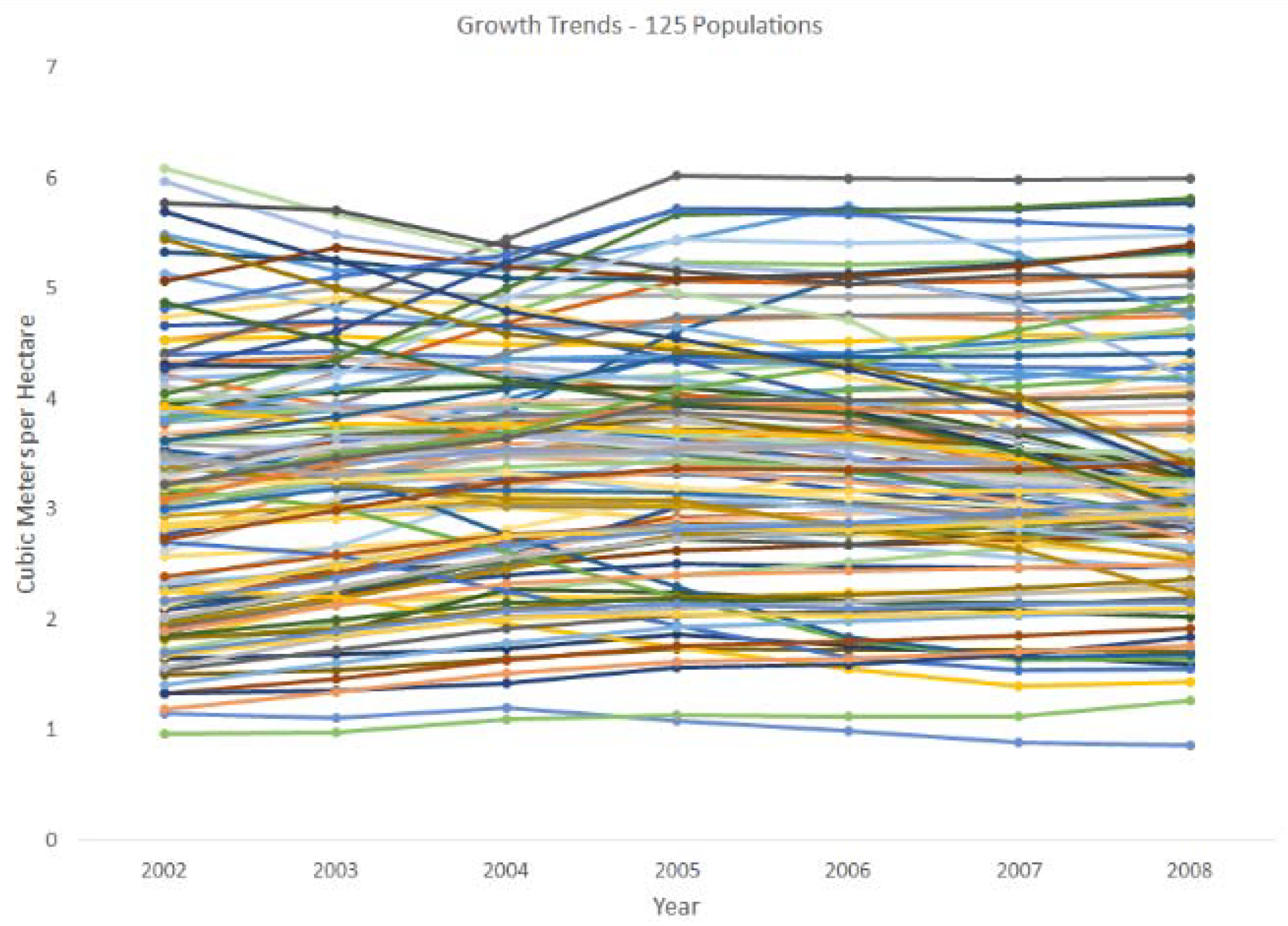
To create a set of populations to test the effects of interval length on the estimates for an intended target length of five years, I expanded the Live growth matrices of 125 of the 152 populations, first described in Roesch et al. [7], and available on DVD from the author upon request. In each population matrix of cubic meter volume growth, each row represents a hectare of land, while each column represents one year, with 21 columns for consecutive years 1995 through 2015. The distribution of population sizes is given in Figure 4, in categories rounded up to the nearest 10,000 hectares. The original matrices were expanded by distributing the annual growth from the original population in a manner intended to mimic intra-annual growth. Each year was split into 10 equal-length segments or decimal years (dy). The actual apportionment of growth to dy within each of the original populations for each year is unknown. Therefore, for simulation purposes, the annual growth was apportioned to dy 1 through 10 of each year in the proportions of 0, 0.05, 0.1, 0.2, 0.2, 0.18, 0.12, 0.1, 0.05, 0. This created 210 columns within each row from the 21 years available (from 1995 through 2015). These populations are being used to examine the effects of many different distributions of interval lengths. In this paper, I discuss the results for a specific set of positively-asymmetric distributions, utilizing five interval lengths of five, six, seven, eight, and nine years, which were sampled in equal proportions in each of the 125 populations. Overall, the combination of these samples is asymmetric from the target interval length of five years. Positively-asymmetric distributions of samples are likely to arise during periods of budget shortfalls if observations are delayed, and are also likely to be problematic for growth estimation. For each interval length, a sample of 1000 rows was taken within each of the 125 populations. This was done for 100 iterations. Five years of observed annualized means from each observation interval length were kept for each expectation viewpoint. For all interval lengths, the annualized means (the mean of the corresponding number of decimal year values times 10) were centralized for the years from 2002 through 2006, and applied to the end of the period for the years 2004 through 2008. The particular years were chosen to accommodate all possible combinations of bases and observation intervals while allowing for the combination of five consecutive panels. In order to give the reader an idea of the diversity of these populations, the true mean trends in cubic meter growth per hectare for the 125 populations over the period of interest (2002–2008) are shown in Figure 5.
Additionally two “fit” datasets were developed using the same methods, one intending to provide weak prior information and one intending to provide strong prior information. The weak fit dataset comprised of a random sample of 100 rows from each population and the strong fit dataset comprised of 5000 rows from each population (five iterations of samples without replacement of 1000 rows each).
Initially, I present the simulation results that are obtained from the treatment of the sample of each interval length as a stand-alone sample. Following that, I combine the samples of the five interval lengths within each population into a single sample for each population in each iteration. I compare the results with respect to three estimands. Estimand 1 corresponds to Expectation (2) with a five-year MidYear basis, Estimand 2 corresponds to Expectation (2) with a five-year EoP basis, and Estimand 3 corresponds to Expectation (3) with a one-year basis.
3. Results
First, I give the simulation results arising from the samples of each interval length, unaided by the prior information. Figure 6 and Figure 7 show the mean bias and mean of the mean squared errors, respectively, for the MidYear means (for years 2002 through 2006) and EoP means (for years 2004–2008) after 100 iterations of samples of size 1000 for each of the five observation interval lengths of five, six, seven, eight, and nine years, within the 125 populations, for Estimands 1 through 3. The values in these figures were developed hierarchically, as simple means of the base statistics. That is, both the simulation bias and MSE were calculated from each sample of size 1000 for each estimate. Then, the means of both statistics were calculated over the 100 iterations for each population. Finally, the means of the population mean bias and mean MSE over the 125 populations were calculated. That is, the mean bias is calculated as:
where nPop is the number of populations (125); nIter is the number of iterations; and is the simulation sample outcome of Estimator E for the variable, X, in population j in a particular year t for iterate i. Similarly, the mean MSE is calculated as:
In Figure 6, it is important to note that the bias of the EoP mean is affected to a much greater extent than that of the MidYear mean, as observation interval length increases from the target interval length. Also, note in the upper right-hand graph, that the least bias is observed for the five-year EoP mean when the observation interval length is exactly five years and Estimand 2, corresponding to a five-year EoP basis. Figure 7 shows that regardless of basis, the MidYear mean results in lower MSEs relative to the EoP mean.
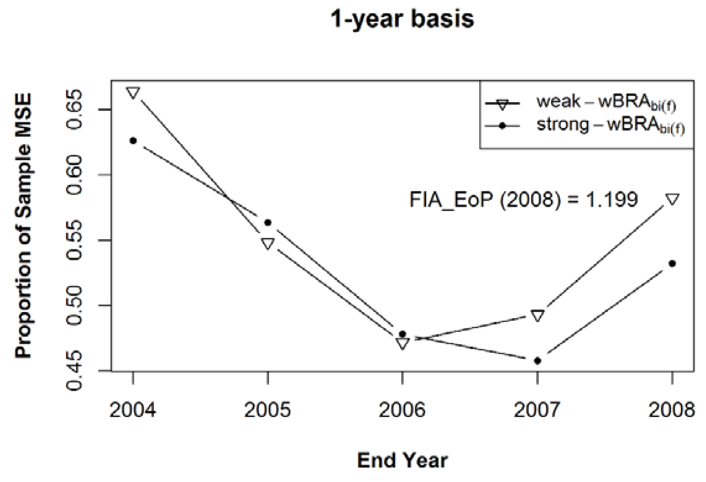
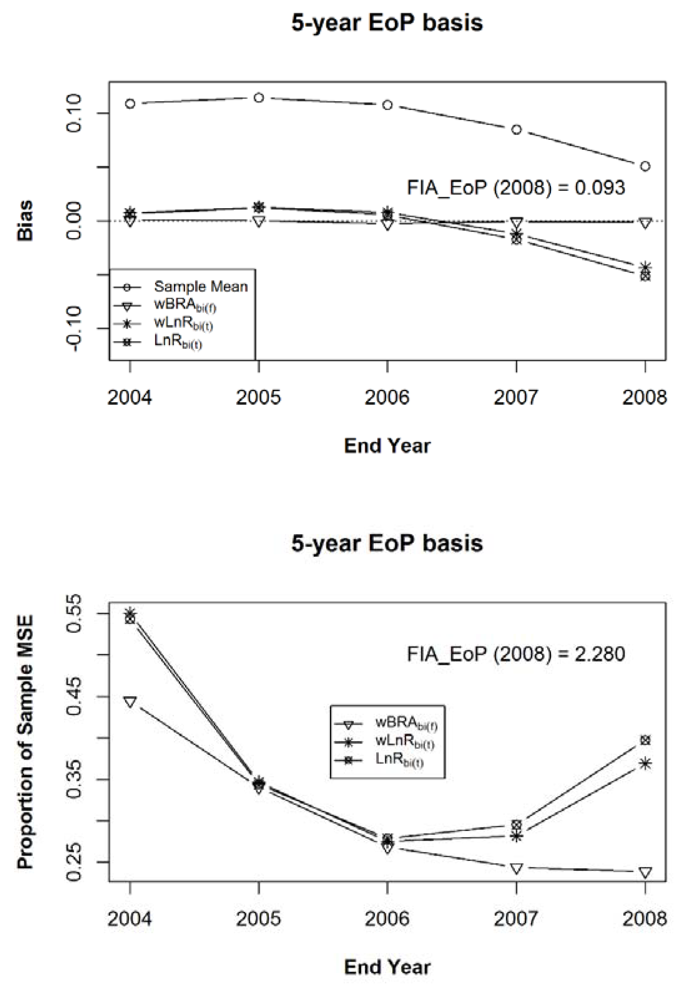
As mentioned above, to compare the various approaches to composite estimator development, I combine the samples of the five interval lengths within each population into a single sample in each iteration. Figure 8, Figure 9 and Figure 10 show, for Estimands 1, 2, and 3, respectively, the simulation mean bias in the top graph and the simulation mean of Mean Squared Errors as a proportion of the MSE of the sample mean in the bottom graph for the bias-adjusted EoP estimator in Equation (8), for years 2004–2008, after adjustment by estimates from the weak and strong prior samples. The methods used to calculate the final values for the simulation mean bias and mean MSE were the same as those used in Figure 6 and Figure 7, except that the initial value for each sample in each population was calculated from the combined sample from all five interval lengths. That is, in contrast to Figure 6 and Figure 7, the summary statistics were compiled after 100 iterations of composite samples, of each of the five (size 1000) samples from each observation length of five, six, seven, eight, and nine years, within each of the 125 populations. The estimand in Figure 8 is Estimand 1, the population’s five-year annualized mean centered on each year of interest, corresponding to Expectation (2) above with a five-year MidYear basis, while the estimand in Figure 9 is Estimand 2, the population’s five-year annualized mean ending on each year of interest, corresponding to Expectation (2) with a five-year EoP basis, and the estimand in Figure 10 is Estimand 3, the population’s annual average for each year of interest, corresponding to Expectation (3). Noteworthy in the bottom graph of all three figures is the significant reduction in MSE achieved by the bias-adjusted estimator under both weak and strong prior information. Figure 9, of course, shows the statistics for the estimator that best matches the pseudo-estimator to the estimand. In the lower graph of that figure, the MSE in the presence of stronger prior information is always lower than it is in the presence of the weaker prior information. The same is not true for Figure 8 and Figure 10, in which the estimator is based on estimands that are not as well matched to the pseudo-estimator. In those same three figures, I also list the simulation mean bias and mean of the mean squared errors (for 2008) for the FIA_EoP estimator, given in Roesch et al. [7], which, in this case, is the mean of five consecutive EoP estimators. The year 2008 is the only year for which the FIA_EoP estimator could be calculated, given the kept simulation results. It is important to note that in all three figures FIA_EoP is more biased and has a higher MSE than the sample mean, due to the known lag bias inherent to that estimator. In this comparison, the sample mean could be viewed as being derived from a single panel, while the FIA_EoP estimator is derived from five consecutive panels. In Figure 9, for 2008, the mean MSE for FIA_EoP is shown to be about seven times higher than under weak prior information and about 10 times higher under strong prior information.
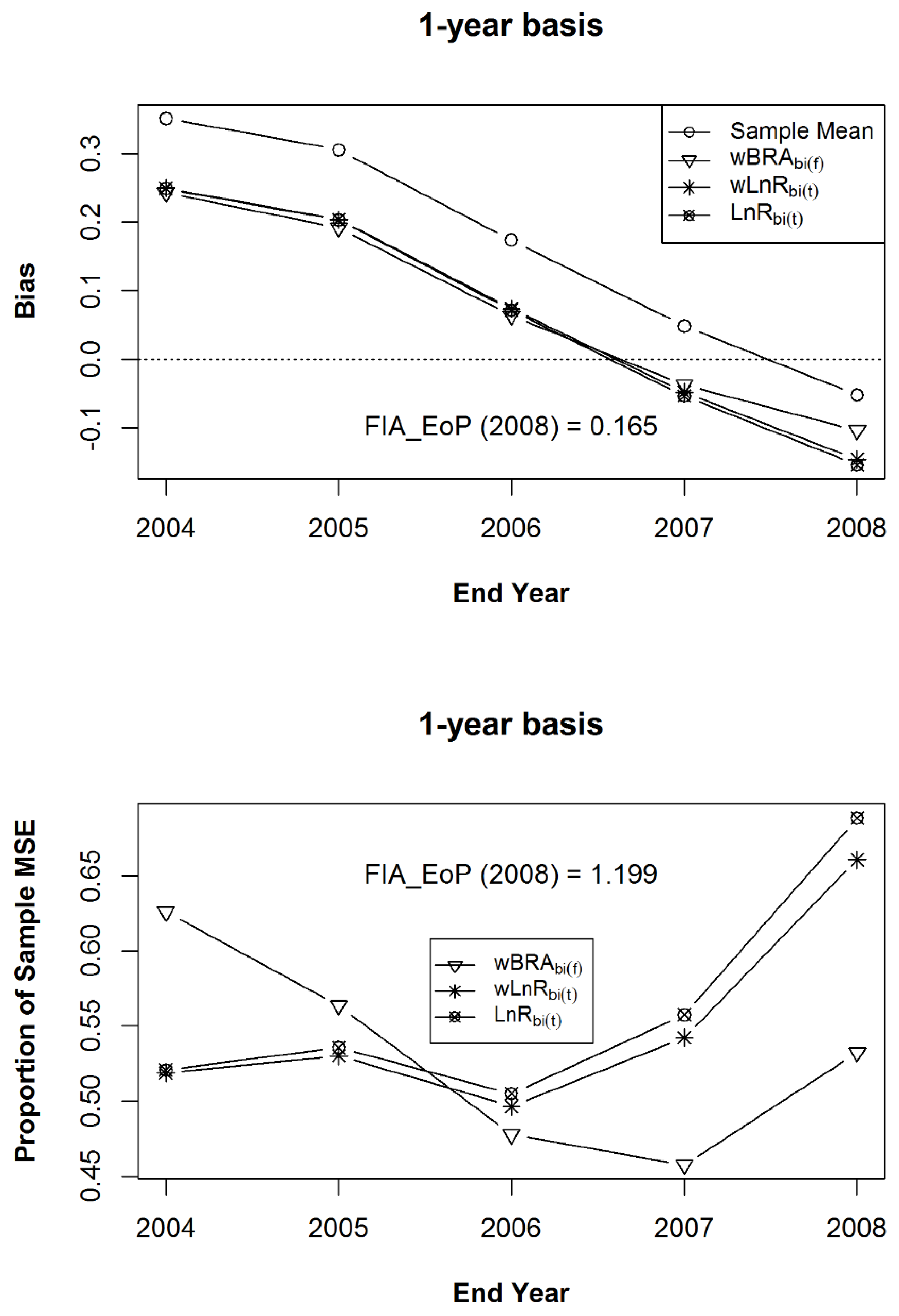
The simulation statistics for the sample mean, (Equation (8)), (Equation (17)), and (Equation (19)), for Estimands 1 through 3, are given in Figure 11, Figure 12 and Figure 13, respectively. The mean bias (a) and the mean of Mean Squared Errors ((b), expressed as a proportion of the MSE of the sample mean) for the bias-adjusted EoP Estimators (for years 2004–2008), using the strong prior sample, after 100 iterations of samples within the 125 populations of a composite sample of sample observation lengths of five, six, seven, eight, and nine years, in equally-sized samples of 1000 rows each. Figure 11 gives the results for Estimand 1, the population’s five-year annualized mean centered on each year of interest which addresses Expectation (2) with a five-year MidYear basis. The results for Estimand 2, the population’s five-year annualized mean ending on each year of interest, are given in Figure 12. Figure 13 presents the results for Estimand 3, the population’s annual average for each year of interest, addressing Expectation (3) with a one-year basis.
4. Discussion
Although I have shown several methods one could use to adjust for the bias in the estimates from alternative interval lengths, I cannot universally claim that the resulting estimators are unbiased. The intent is for them to be less biased. Admittedly, these methods are coarse. However, in the simulation above, they are shown to be useful. Estimation of the bias can be problematic because sometimes there are very few observations on interval lengths that equal the basis of interest, so often there is no low-variance estimate of the target mean. Additionally, I note several related points made in a series of papers (Green and Strawderman [6,8,9]): the first being that often (as is the case here for alternative interval lengths), there is not an optimal way to estimate the bias (and therefore the MSE), and the second being that as the bias increases, the risk of the Composite estimator, under squared-error loss, increases and is unbounded.
A major problem that is being addressed here is not rare: a user of any publicly available data or analysis must often assume an estimand based on a governmental entity’s description of its data aggregation procedures. In the case of FIA data, I have shown that this user’s dilemma can be, at least partially, addressed through the provision of a set of well-defined target estimands. What I am suggesting, but have not shown (because it is an immediate result in statistical theory), is that if a user can establish a theoretical population link between their own estimand of choice and one previously provided, then there is a chance of developing an estimator with acceptable statistical properties. As mentioned earlier, clarity in the definition of the estimand is necessary in order for one to have defined an estimator, and to evaluate the statistical properties of that estimator. The establishment of a set of target estimands at least provides a user with a method to evaluate the relationship between the user’s expectations and the information being provided by the public entity.
5. Conclusions
The positively-asymmetric measurement intervals simulated here represent a potential effect of an unplanned reduction of sampling effort, such as what might be necessitated by a reduction in budget being applied to a national forest inventory. This is a complicating factor, but it is the definition of the estimand that lends clarity to exactly what is being complicated. For instance, observing a growth rate over a series of seven-year intervals as opposed to a series of five-year intervals obviously does not change the growth rate with respect to a five-year basis, but it does complicate one’s attempt to estimate the growth rate with respect to a five-year basis. If we frame all discussions and analyses simply in terms of an “average annual growth,” we lose that clarity. What has been shown here are a few of the many approaches that could be used to both maintain that clarity and still fully utilize an extremely rich but somewhat recalcitrant data set.
Funding
Funding for this research was provided by the author’s employer, the USDA Forest Service, Southern Research Station, Forest Inventory and Analysis Unit, Knoxville, TN, USA.
Acknowledgments
This manuscript was improved through the incorporation of review comments offered by Kathryne Roesch, William G. Burkman, and two anonymous reviewers.
Conflicts of Interest
The author declares no conflict of interest. The funders had no role in the design of the study; in the collection, analyses, or interpretation of data; in the writing of the manuscript, and in the decision to publish the results.
References
- Ott, L. An Introduction to Statistical Methods and Data Analysis; Duxbury Press: North Scituate, MA, USA, 1977; 730p. [Google Scholar]
- Bechtold, W.A.; Patterson, P.L. The Enhanced Forest Inventory and Analysis Program-National Sampling Design and Estimation Procedures; U.S. Department of Agriculture Forest Service, Southern Research Station: Asheville, NC, USA, 2005. Available online: http://www.srs.fs.fed.us/pubs/20371 (accessed on 1 February 2018).
- Mood, A.M.; Graybill, F.A.; Boes, D.C. Introduction to the Theory of Statistics, 3rd ed.; McGraw-Hill, Inc.: New York, NY, USA, 1974; 564p. [Google Scholar]
- Roesch, F.A.; Van Deusen, P.C. Time as a Dimension of the Sample Design in National Scale Forest Inventories. For. Sci. 2013, 59, 610–622. [Google Scholar] [CrossRef]
- Roesch, F.A. The components of change for an annual forest inventory design. For. Sci. 2007, 53, 406–413. [Google Scholar]
- Green, E.J.; Strawderman, W.E. Combining inventory estimates with possibly biased auxiliary information. For. Sci. 1990, 36, 693–704. [Google Scholar]
- Roesch, F.A.; Schroeder, T.C.; Vogt, J.T. Effects of Cycle Length and Plot Density on Estimators for a National-Scale Forest Monitoring Sample Design. Forests 2017, 8, 325. [Google Scholar] [CrossRef]
- Green, E.J.; Strawderman, W.E. Combining Inventory Data with Model Predictions. In Proceedings of the Forest Growth Modelling and Prediction Conference, Minneapolis, MN, USA, 23–27 August 1987; pp. 676–682. [Google Scholar]
- Green, E.J.; Strawderman, W.E. A James-Stein type estimator for combining unbiased and possibly-biased estimators. JASA 1991, 86, 1000–1006. [Google Scholar] [CrossRef]
Figure 1.
The interval length distribution of one-year categories in FIADB for 34 States in the United States, with the end-of-interval measurement made between 1998 and 2016.
Figure 1.
The interval length distribution of one-year categories in FIADB for 34 States in the United States, with the end-of-interval measurement made between 1998 and 2016.
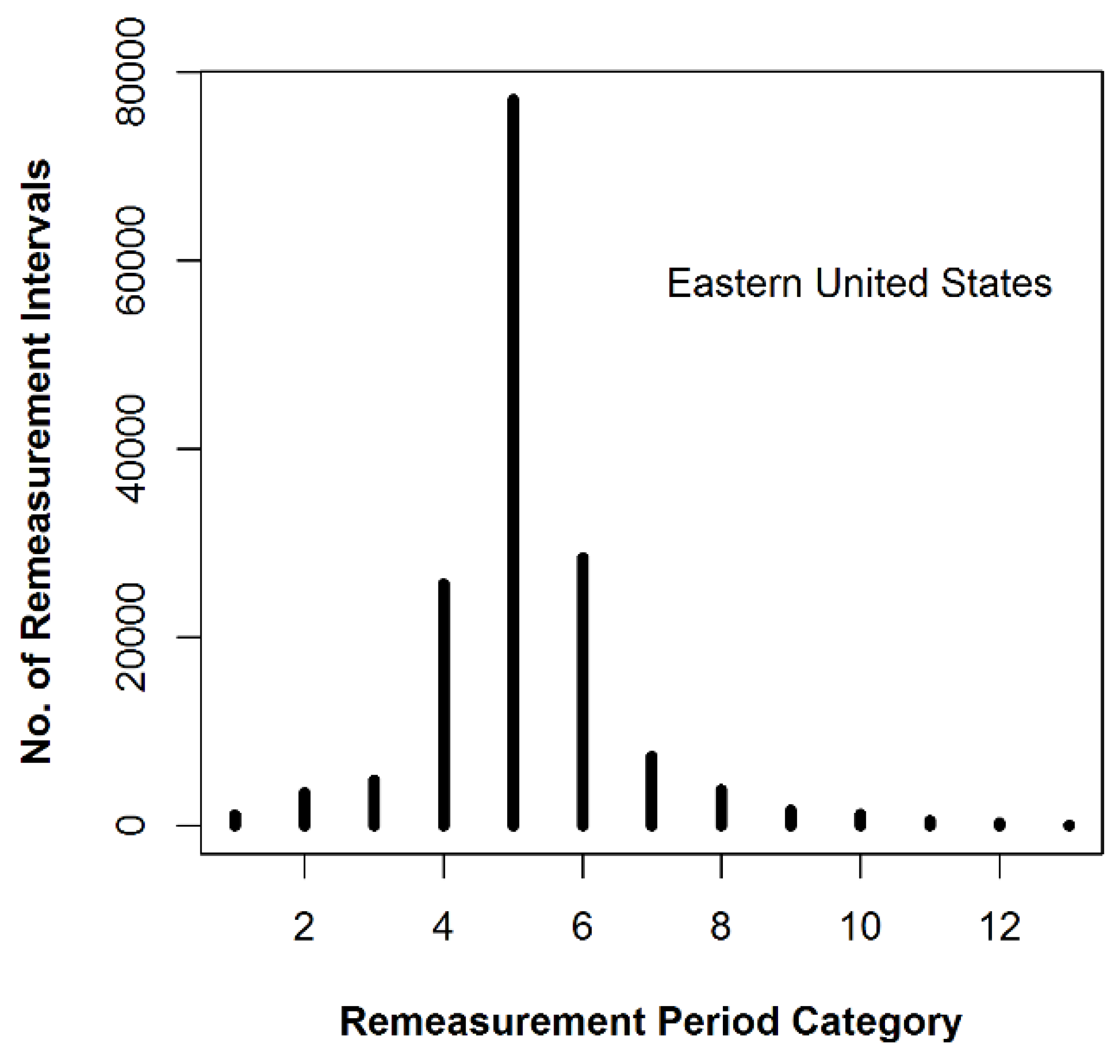
Figure 2.
The interval length distribution of one-year categories (of one to 13 years) in FIADB for 34 States in the United States, by MidYear ranging from 1996 to 2014.
Figure 2.
The interval length distribution of one-year categories (of one to 13 years) in FIADB for 34 States in the United States, by MidYear ranging from 1996 to 2014.

Figure 3.
The interval length one-year categorical distributions in FIADB for 34 States in the United States, listed by the two digit State Codes given in Table 1, for MidYears ranging from 1996 to 2014.
Figure 3.
The interval length one-year categorical distributions in FIADB for 34 States in the United States, listed by the two digit State Codes given in Table 1, for MidYears ranging from 1996 to 2014.
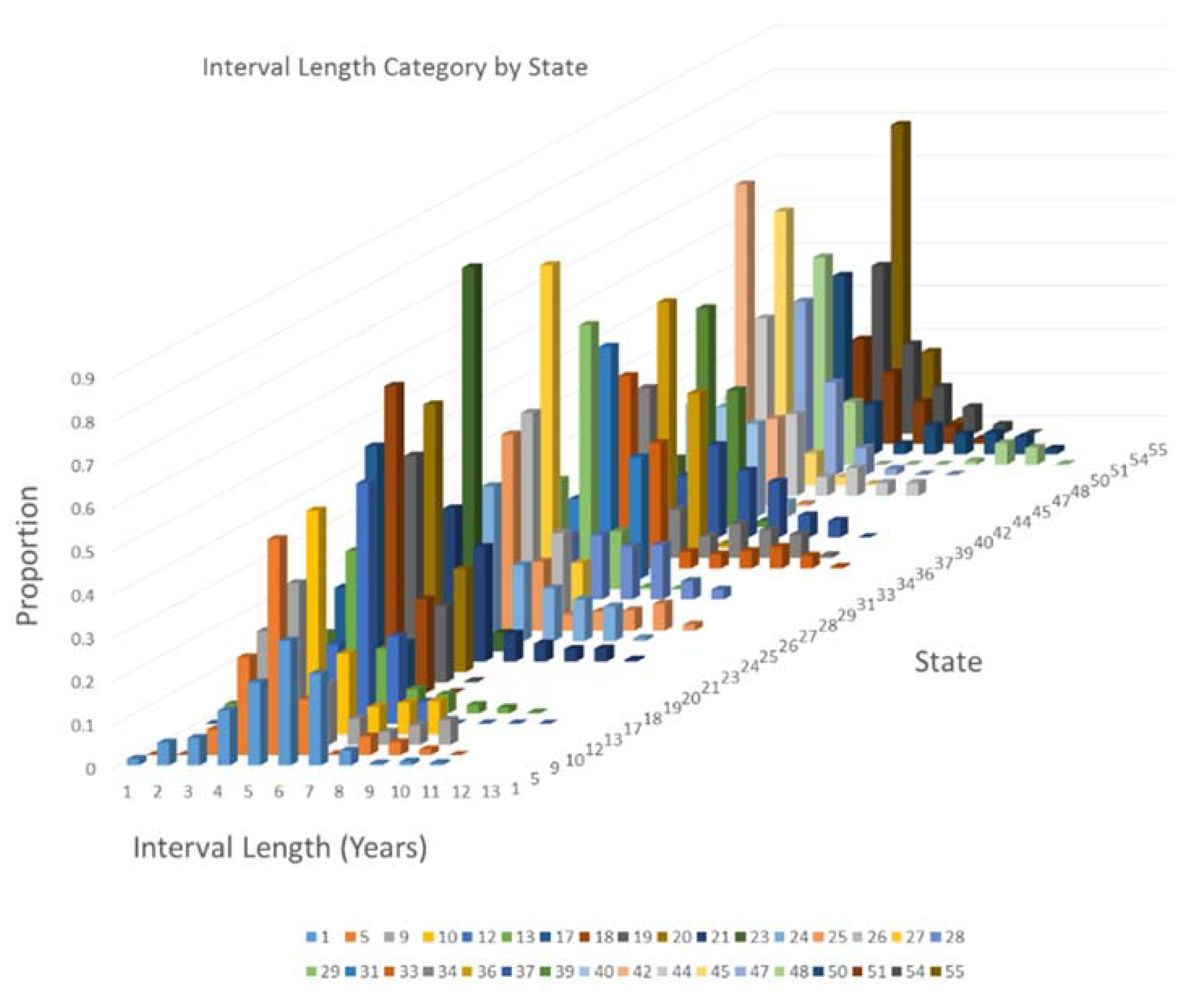
Figure 4.
The distribution of population sizes for the 125 populations in the simulation in categories rounded up to the nearest 10,000 Hectares.
Figure 4.
The distribution of population sizes for the 125 populations in the simulation in categories rounded up to the nearest 10,000 Hectares.

Figure 5.
The mean trend in cubic meter growth per hectare per year for each of the 125 populations over the period of 2002 through 2008.
Figure 5.
The mean trend in cubic meter growth per hectare per year for each of the 125 populations over the period of 2002 through 2008.

Figure 6.
The mean bias for the MidYear annual mean (for years 2002 through 2006) and the EoP annual mean Estimators (for years 2004–2008) after 100 iterations of samples of size 1000 within the 125 populations, for sample observation lengths of five, six, seven, eight, and nine years, respectively. Each graph is relative to a unique estimand: (a) Estimand 1 with a five-year MidYear basis; (b) Estimand 2 with a five-year EoP basis; (c) Estimand 3 with a one-year basis.
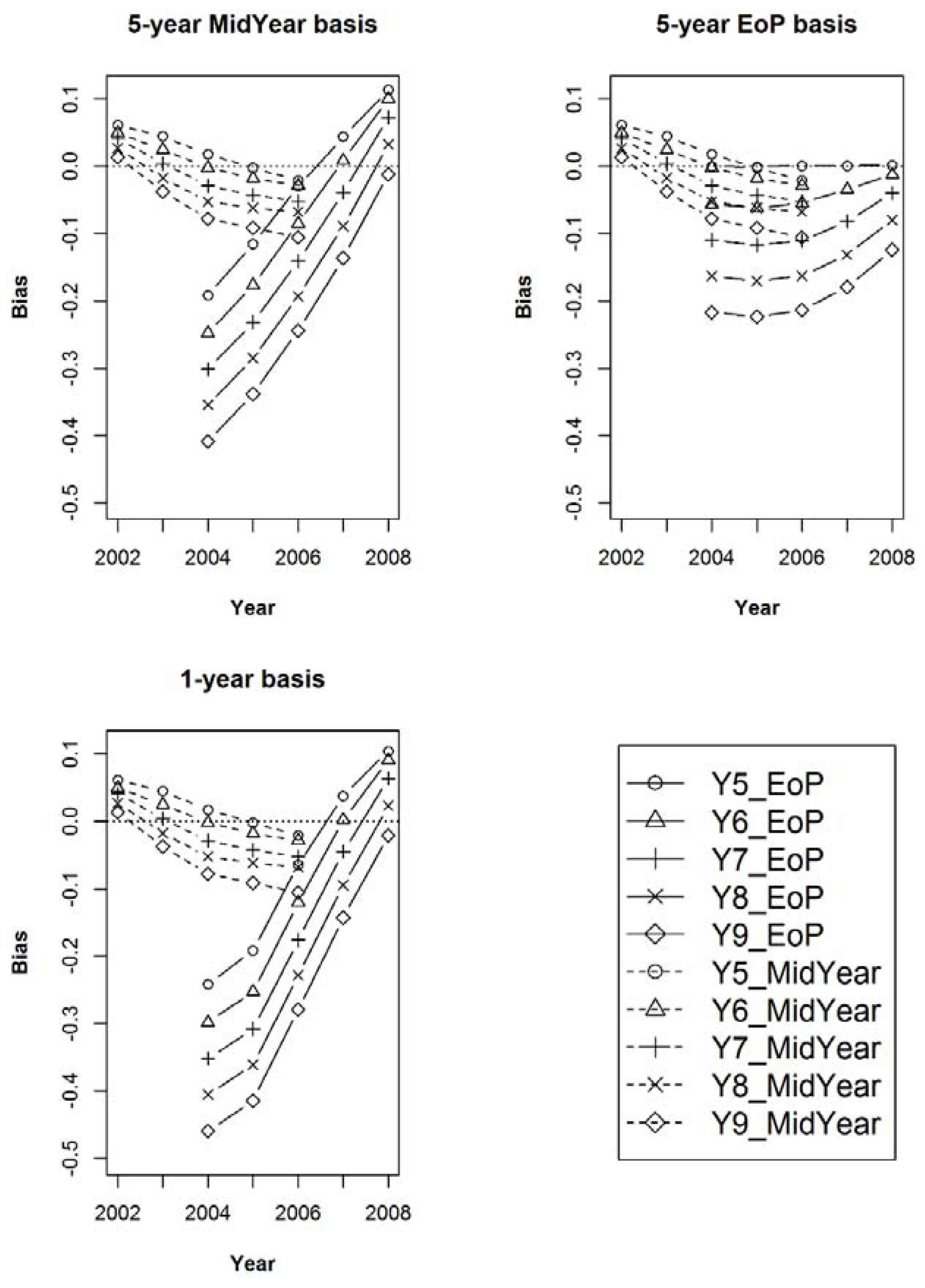
Figure 7.
The mean of the Mean Squared Errors (MSE) for the MidYear annual mean (for years 2002 through 2006) and the EoP annual mean Estimators (for years 2004–2008) after 100 iterations of samples of size 1000 within the 125 populations, for sample observation lengths of five, six, seven, eight, and nine years, or deviations (from 50 dy) of 0, 10, 20, 30, and 40, respectively. As in Figure 6, each graph is relative to a unique estimand: (a) Estimand 1 with a five-year MidYear basis; (b) Estimand 2 with a five-year EoP basis; (c) Estimand 3 with a one-year basis.
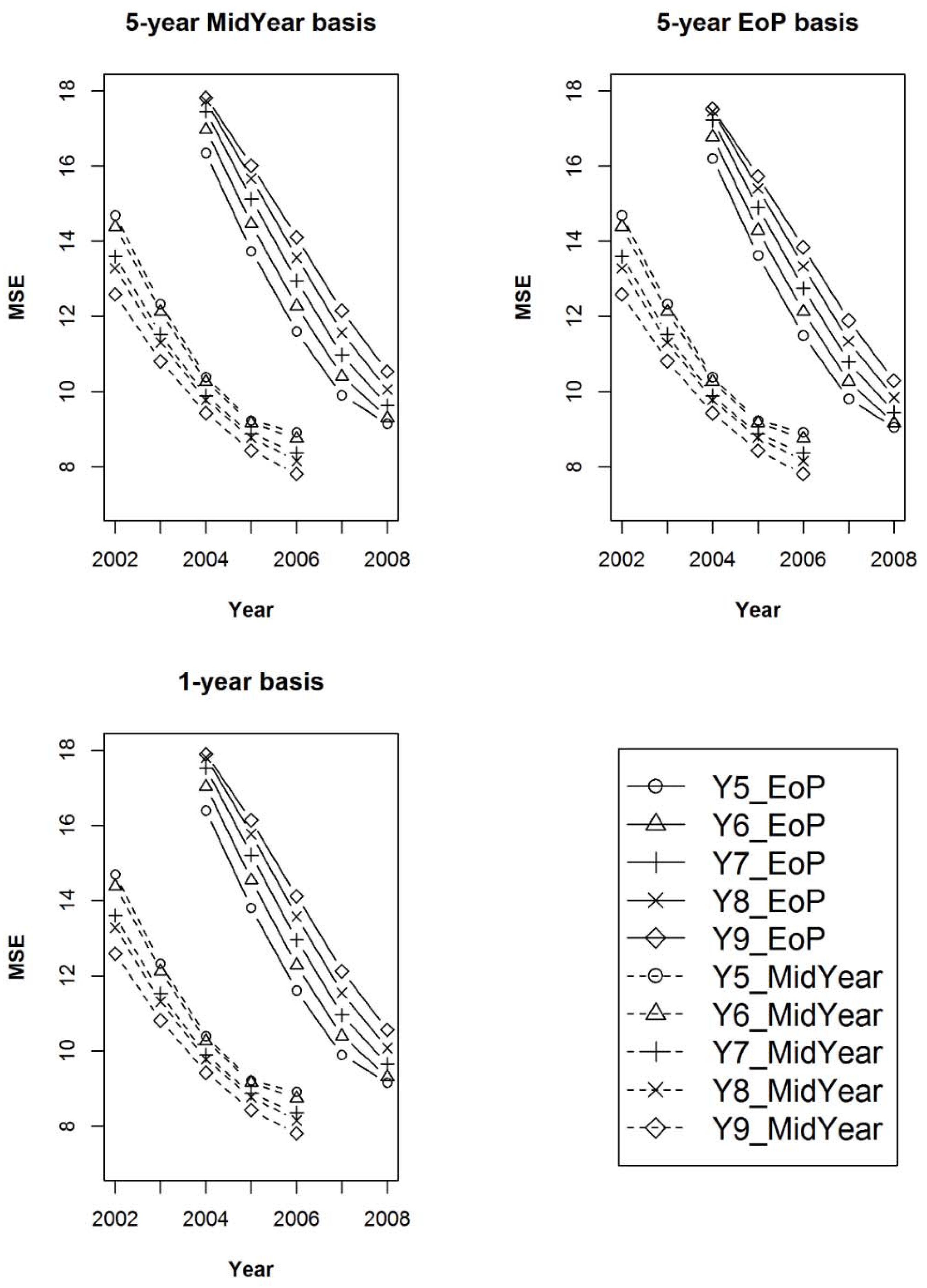
Figure 8.
The mean bias (a) and the mean of Mean Squared Errors ((b), expressed as a proportion of the MSE of the sample mean), relative to Estimand 1, for the bias-adjusted EoP Estimator (for years 2004–2008), using the weak and strong prior samples, as described in the text, after 100 iterations of samples of size 1000 within the 125 populations of a composite sample of sample observation lengths of five, six, seven, eight, and nine years, in equal proportions.
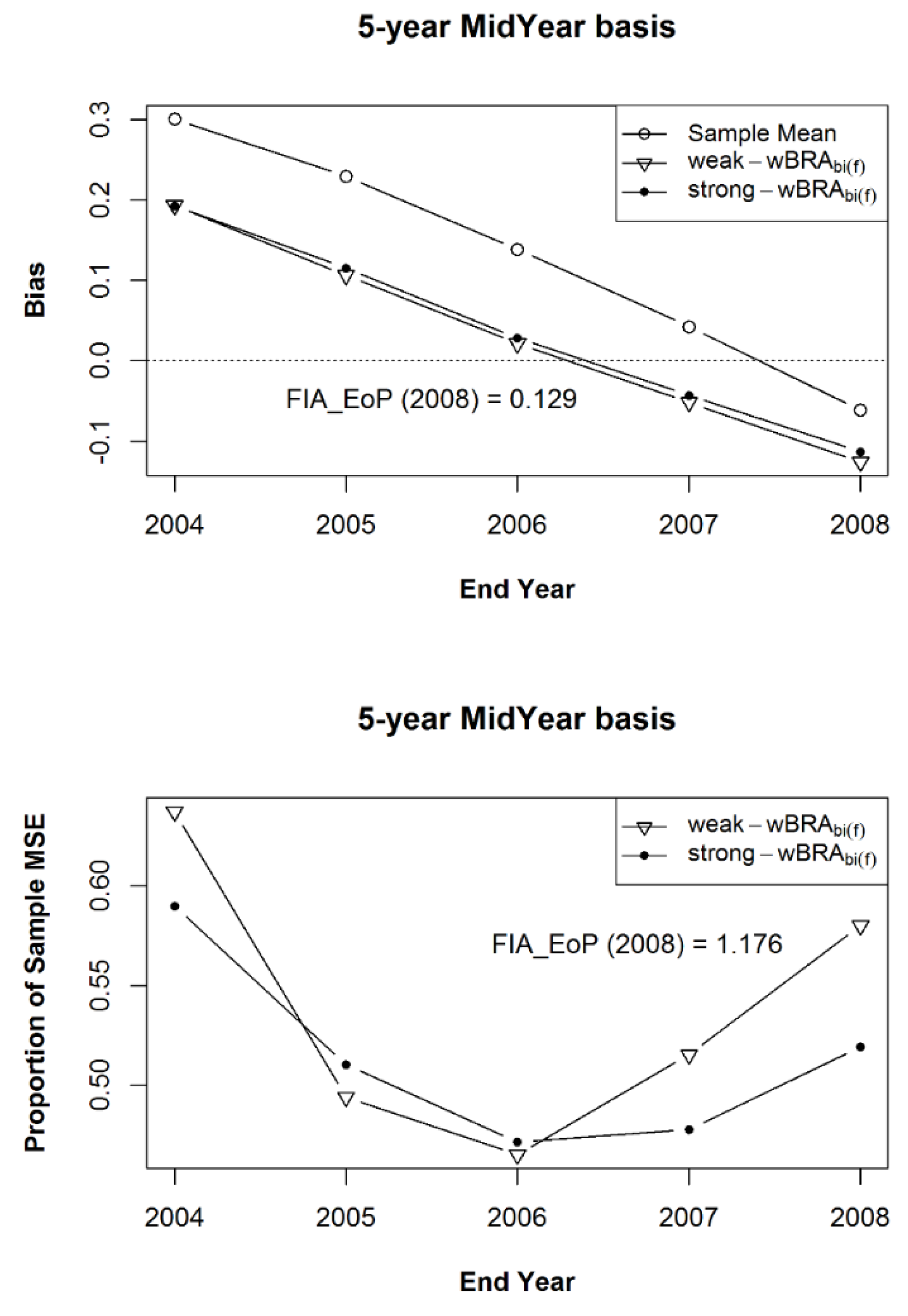
Figure 9.
The simulation mean bias (a) and the mean of Mean Squared Errors ((b), expressed as a proportion of the MSE of the sample mean) for Estimand 2 and the bias-adjusted EoP Estimator (for years 2004–2008), using the weak and strong prior samples after 100 iterations of samples of size 1000 within the 125 populations of a composite sample of sample observation lengths of five, six, seven, eight, and nine years, in equal proportions.
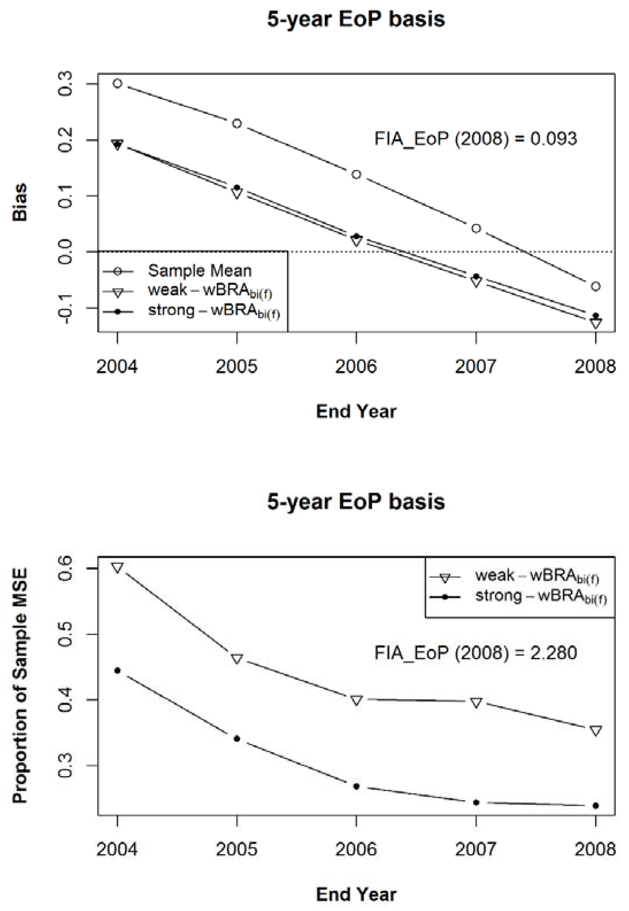
Figure 10.
The mean bias (a) and the mean of Mean Squared Errors ((b), expressed as a proportion of the MSE of the sample mean) for the bias-adjusted EoP Estimator (for years 2004–2008), relative to Estimand 3, using the weak and strong prior samples, after 100 iterations of samples of size 1000 within the 125 populations of a composite sample of sample observation lengths of five, six, seven, eight, and nine years, in equal proportions.
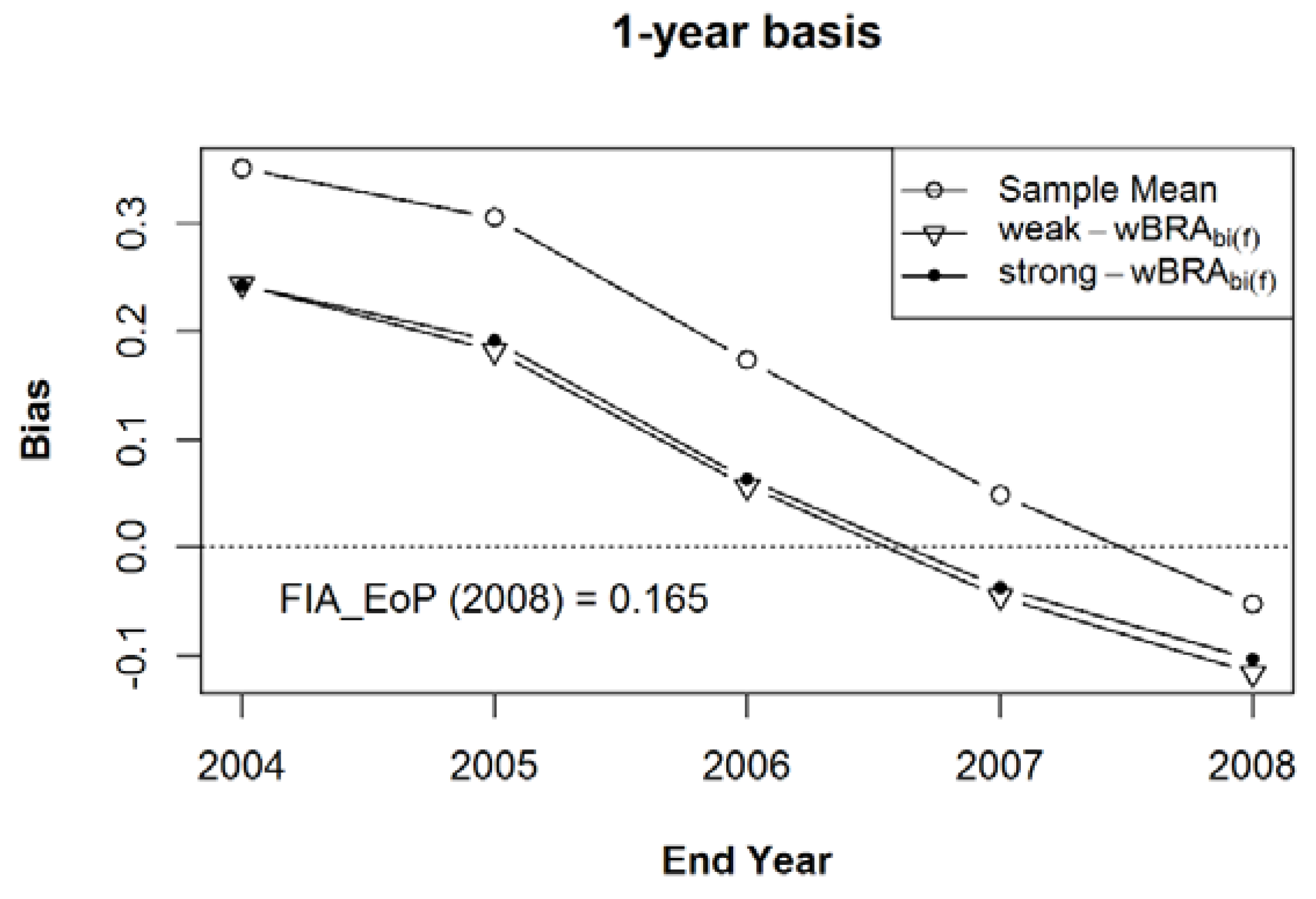

Figure 11.
The mean bias (a) and the mean of Mean Squared Errors ((b), expressed as a proportion of the MSE of the sample mean), relative to Estimand 1, for the bias-adjusted EoP estimators (for years 2004–2008), using the strong prior sample, after 100 iterations of samples of size 1000 within the 125 populations of a composite sample of sample observation lengths of five, six, seven, eight, and nine years, in equal proportions.
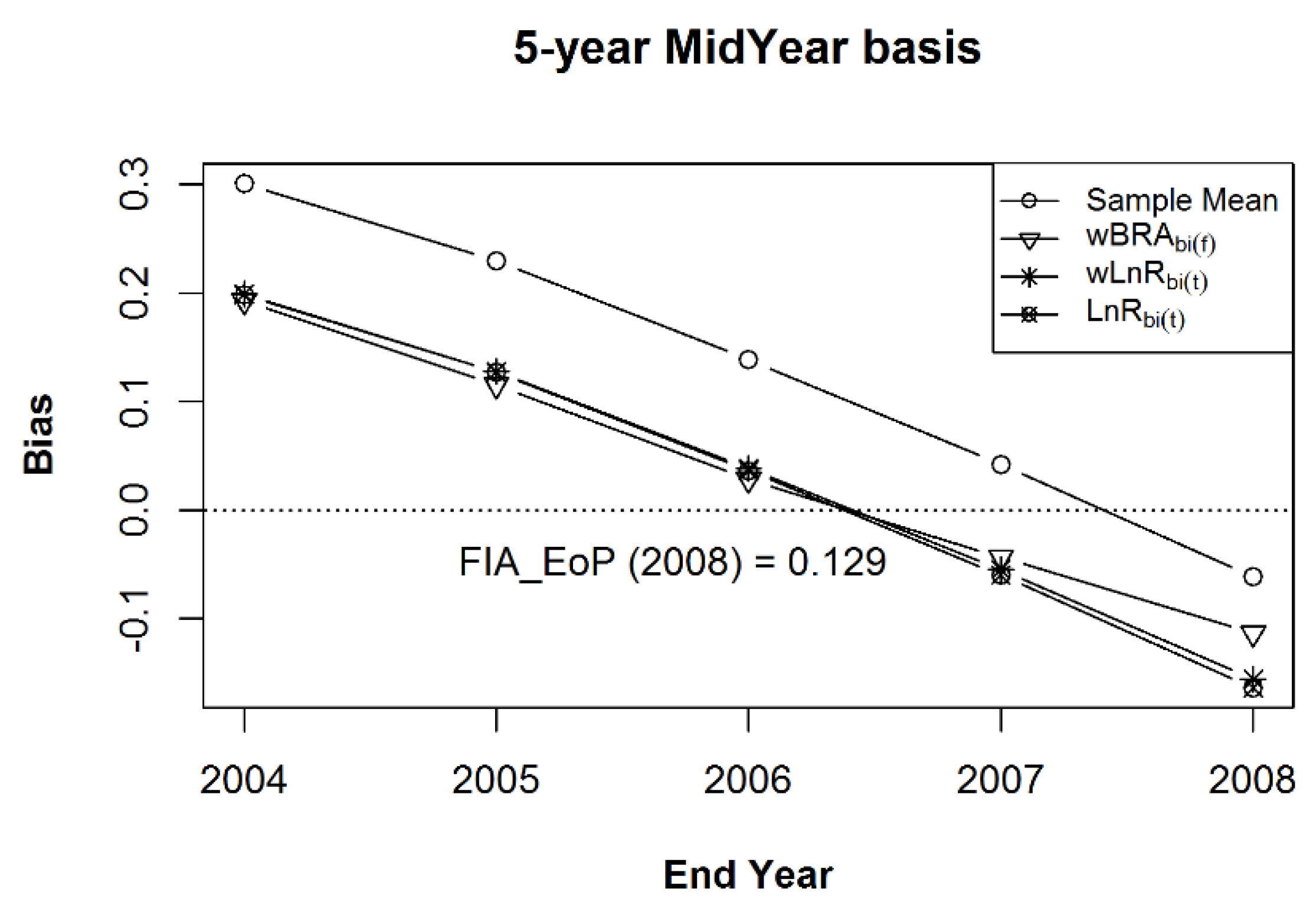
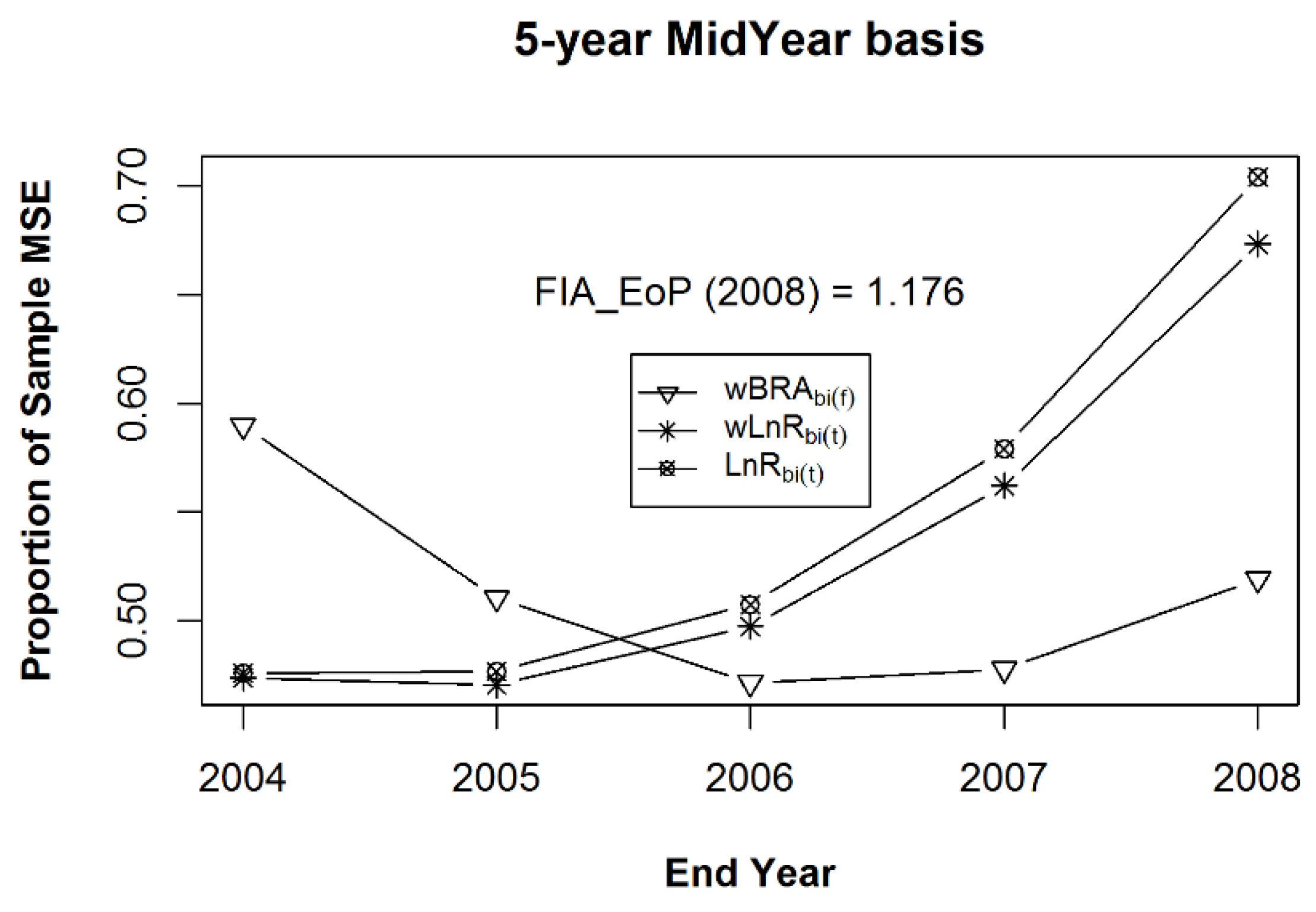
Figure 12.
For Estimand 2, the mean bias (a) and the mean of Mean Squared Errors ((b), expressed as a proportion of the MSE of the sample mean) for the bias-adjusted EoP estimators (for years 2004–2008), using the strong prior sample, after 100 iterations of samples of size 1000 within the 125 populations of a composite sample of sample observation lengths of five, six, seven, eight, and nine years, in equal proportions.

Figure 13.
The mean bias (a) and the mean of Mean Squared Errors ((b), expressed as a proportion of the MSE of the sample mean), relative to Estimand 3, for the bias-adjusted EoP estimators (for years 2004–2008), using the strong prior sample, after 100 iterations of samples of size 1000 within the 125 populations of a composite sample of sample observation lengths of five, six, seven, eight, and nine years, in equal proportions.


Table 1.
State Codes in the USDA Forest Service Forest Inventory and Analysis Database (FIADB) for the States used in this study.
Table 1.
State Codes in the USDA Forest Service Forest Inventory and Analysis Database (FIADB) for the States used in this study.
| State Code | State Name | Abbreviation |
|---|---|---|
| 1 | Alabama | AL |
| 5 | Arkansas | AR |
| 9 | Connecticut | CT |
| 10 | Delaware | DE |
| 12 | Florida | FL |
| 13 | Georgia | GA |
| 17 | Illinois | IL |
| 18 | Indiana | IN |
| 19 | Iowa | IA |
| 20 | Kansas | KS |
| 21 | Kentucky | KY |
| 23 | Maine | ME |
| 24 | Maryland | MD |
| 25 | Massachusetts | MA |
| 26 | Michigan | MI |
| 27 | Minnesota | MN |
| 28 | Mississippi | MS |
| 29 | Missouri | MO |
| 31 | Nebraska | NE |
| 33 | New Hampshire | NH |
| 34 | New Jersey | NJ |
| 36 | New York | NY |
| 37 | North Carolina | NC |
| 39 | Ohio | OH |
| 40 | Oklahoma | OK |
| 42 | Pennsylvania | PA |
| 44 | Rhode Island | RI |
| 45 | South Carolina | SC |
| 47 | Tennessee | TN |
| 48 | Texas | TX |
| 50 | Vermont | VT |
| 51 | Virginia | VA |
| 54 | West Virginia | WV |
| 55 | Wisconsin | WI |
© 2018 by the author. Licensee MDPI, Basel, Switzerland. This article is an open access article distributed under the terms and conditions of the Creative Commons Attribution (CC BY) license (http://creativecommons.org/licenses/by/4.0/).
Share and Cite
MDPI and ACS Style
Roesch, F.A. Composite Estimators for Growth Derived from Repeated Plot Measurements of Positively-Asymmetric Interval Lengths. Forests 2018, 9, 427. https://doi.org/10.3390/f9070427
AMA Style
Roesch FA. Composite Estimators for Growth Derived from Repeated Plot Measurements of Positively-Asymmetric Interval Lengths. Forests. 2018; 9(7):427. https://doi.org/10.3390/f9070427
Chicago/Turabian StyleRoesch, Francis A. 2018. "Composite Estimators for Growth Derived from Repeated Plot Measurements of Positively-Asymmetric Interval Lengths" Forests 9, no. 7: 427. https://doi.org/10.3390/f9070427
Note that from the first issue of 2016, this journal uses article numbers instead of page numbers. See further details here.