Modeling Burned Areas in Indonesia: The FLAM Approach
by
 , , , and
Andrey Krasovskii
* ,
,
Nikolay Khabarov
,
Johannes Pirker
,
Florian Kraxner
,
Ping Yowargana
,
Dmitry Schepaschenko
 and
and
Michael Obersteiner
Ecosystems Services & Management (ESM) Program, International Institute for Applied Systems Analysis (IIASA), Schlossplatz 1, A-2361 Laxenburg, Austria
*
Author to whom correspondence should be addressed.
Forests 2018, 9(7), 437; https://doi.org/10.3390/f9070437
Submission received: 20 June 2018
/
Revised: 16 July 2018
/
Accepted: 18 July 2018
/
Published: 20 July 2018
(This article belongs to the Special Issue Managing Wildfires in Changing Climates: History, Current Practice, and Challenges)
Abstract
:Large-scale wildfires affect millions of hectares of land in Indonesia annually and produce severe smoke haze pollution and carbon emissions, with negative impacts on climate change, health, the economy and biodiversity. In this study, we apply a mechanistic fire model to estimate burned area in Indonesia for the first time. We use the Wildfire Climate Impacts and Adaptation Model (FLAM) that operates with a daily time step on the grid cell of 0.25 arc degrees, the same spatio-temporal resolution as in the Global Fire Emissions Database v4 (GFED). GFED data accumulated from 2000–2009 are used for calibrating spatially-explicit suppression efficiency in FLAM. Very low suppression levels are found in peatland of Kalimantan and Sumatra, where individual fires can burn for very long periods of time despite extensive rains and fire-fighting attempts. For 2010–2016, we validate FLAM estimated burned area temporally and spatially using annual GFED observations. From the validation for burned areas aggregated over Indonesia, we obtain Pearson’s correlation coefficient separately for wildfires and peat fires, which equals 0.988 in both cases. Spatial correlation analysis shows that in areas where around 70% is burned, the correlation coefficients are above 0.6, and in those where 30% is burned, above 0.9.
1. Introduction
Fires affect terrestrial ecosystems and have profound consequences on global climate, air quality and vegetation [1,2]. Fire regimes are determined by climate variability, vegetation and direct human influence. Seasonal weather is the most variable factor and has the greatest effect on regional burned area [3,4]. Climate change lengthens fire seasons, with an associated trend towards increasing extent, frequency and severity of fires, as well as the global occurrence of extreme (mega) fire events [5] in many regions of the Earth (e.g., in the Mediterranean [6] and boreal [7] regions). At the same time, human activity is the primary source of ignition in global forest, savanna and agricultural regions. Indonesia is one of the countries that has experienced particularly large-scale peatland and forest fire disasters [8]. According to the World Bank [9], 2.6 million hectares of Indonesian land burned between June and October 2015, costing Indonesia USD 16.1 billion.
Most fires in Indonesia are induced by human activity [9]. Forest and land clearing for plantations and agriculture have been cited by various researchers as the major causes of these fires [10]. Indonesia contains 47% of the global area of tropical peatland, located mostly in peat swamp forest [11]. Large peatland areas have been converted to agriculture, initially under the Indonesian Government’s transmigration program, and later for commercial oil palm and paper pulp tree plantations, especially in Sumatra and Kalimantan [12,13]. Draining and conversion of peatland, driven largely by palm oil production, contributes to the intensity of haze from fire [9]. Peatlands account for about one-third of the area burned, but are responsible for the vast majority of the haze and CO emissions from the fires [9].
Fires have a large disruptive impact in Indonesia, affecting millions of hectares of land, producing severe smoke haze pollution. There are multiple negative effects of wildfires in Indonesia on climate change [14], health [15], the economy [8,9] and biodiversity (http://fires.globalforestwatch.org/about/). Indonesia’s biomass burning emissions are comparable to the annual fossil fuel CO emissions of countries such as Japan and India [16,17].
The overall fire situation in Indonesia is described in various papers [18,19]. In this study, we apply a mechanistic wildfire model to estimate burned area in Indonesia. Fire models are developed for hazard assessment, as well as forest and fuel management planning, including prescribed burning and suppression efforts. The paper led by Herawati [20] reviewed available fire models (e.g., the Risco de Queimada/fire risk model (RisQue), Coupled Atmosphere-Wildland Fire-Environment (CAWFE) and FireFamilyPlus), which could be potentially used in Indonesia. However, we have not come across a mechanistic model that specifically focuses on modeling burned areas in the forest and peatland of Indonesia in the literature. This motivated us to apply the Wildfire Climate Impacts and Adaptation Model (FLAM) to modeling burned areas in Indonesia, as described in this paper.
There have been studies from different territories where historical climate data in combination with Moderate Resolution Imaging Spectroradiometer (MODIS) satellite data were used in fire mapping [21,22]. However, they did not deal with explicit modeling of burned areas. At the same time, area burned is the most commonly-used indicator when fire trends are being examined [23], and the assessment of burned area is an important step in estimating the cost of fire [9], as well as the air quality impacts [24]. Previously in studies led by Khabarov [25] and Krasovskii [26], FLAM (formerly known as the Standalone Fire Model (SFM)) was applied to modeling burned areas in Europe. In this study, we enhance the model by estimating several wildfire process parameters to better fit regional conditions in Indonesia. For the purposes of this paper, we separate peat fires from wildfires.
Methodologically, our paper contributes to the development of the original algorithm by Arora and Boer [27]. In a recent study, Arora and Melton [28] linked fire extinguishing probability with population density. We demonstrate that this simplified approach can be improved by an explicit calibration of suppression efficiency.
In this paper, we test the following hypotheses: (1) the observed burned area in Indonesia reported by the Global Fire Emission Dataset (GFED) [29] (which is based on satellite observations) can be modeled independently by FLAM; (2) the approach integrating the Canadian Fire Weather Index (FWI) [30,31,32] into a mechanistic fire model provides good accuracy in assessment of burned area; (3) the spatial suppression efficiency calibrated using observed burned area improves the original fire algorithm for area burned by wildfires and peat fires.
2. Materials and Methods
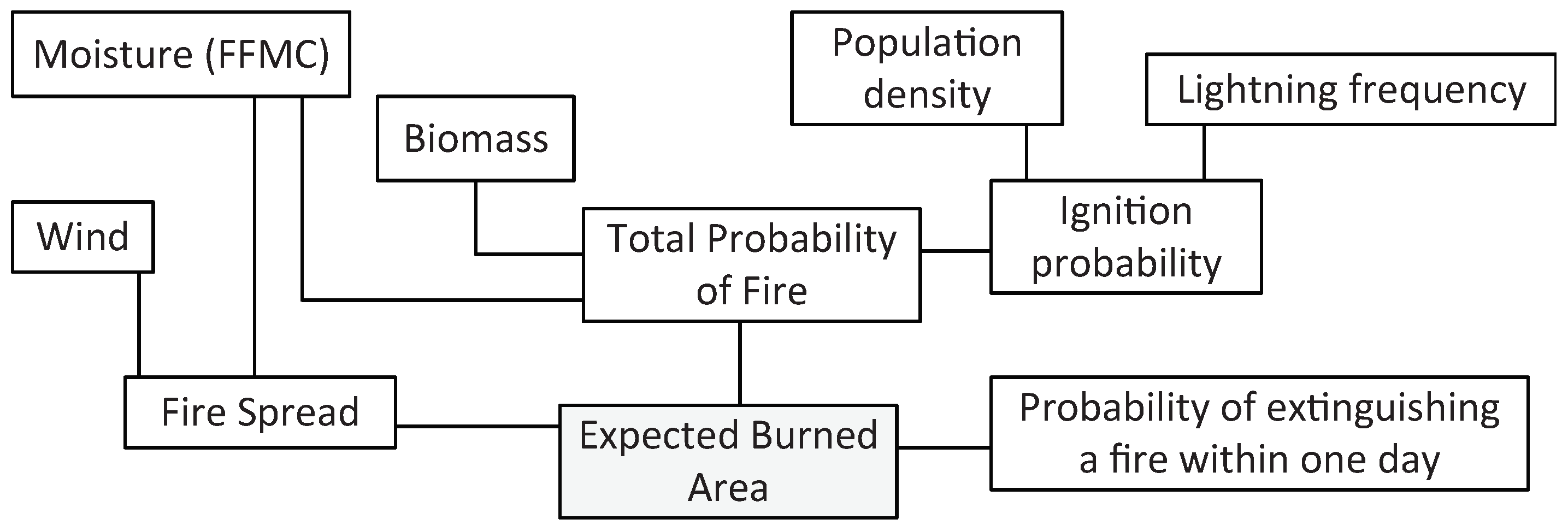
FLAM is used to reproduce historical and to project future burned area, as well as to assess climate change impacts and adaptation options (http://www.iiasa.ac.at/flam). FLAM is able to capture impacts of climate, human activity and fuel availability on burned areas. It uses a process-based fire parametrization algorithm that was developed to link a fire model with the Dynamic Global Vegetation Models (DGVMs) in the literature [27,28,33,34,35,36]. FLAM is a standalone fire model based on the Arora and Boer [27] algorithm, being decoupled from DGVM. This allows for faster running times and application of the calibration approach, described below. The key features implemented in FLAM include fuel moisture computation based on the Fine Fuel Moisture Code (FFMC) of the Canadian FWI [30] and a procedure to calibrate regional fire suppression efficiency as proposed in previous studies [25,26].
The FLAM flowchart is depicted in Figure 1. The model operates with a daily time-step at 0.25-arc degree spatial resolution. All inputs were re-sampled to fit the model resolution, using the resample and aggregate functions of the raster package [37] in the R software; we used the country shape of Indonesia from the wrld_simpl dataset available in R.
To model daily fire occurrences, FLAM computes three conditional probabilities of fire:
- probability of ignition depending on natural and human sources
- probability of ignition subject to fuel availability
- probability of ignition depending on weather
2.1. Ignition Probability
There are two causes of ignition: (i) natural and (ii) human activity. Natural ignition is represented in the model by lightning frequency. Our approach to modeling human ignition and suppression consists of two steps. Firstly, we use a standard procedure, where population density is transformed into probability functions of human ignition and simultaneously suppression [35], i.e., “unsuppressed ignition”. Secondly, we apply a calibration procedure that identifies pixels with higher or lower suppression efficiency [26], i.e., probability of extinguishing a fire within one day, based on observed burned areas. In the case when the calibrated probability in a pixel equals one, the fire is suppressed “immediately”. Thus, observations help us to additionally identify the human activity impact independently from population density.
In this study, population density was taken from the dynamic maps of the Gridded Population of the World, v4 [38]. We used maps for the years 2000, 2005, 2010 and 2015, inside the modeling interval 2000–2016. Original data were averaged using the mean function excluding empty data cells. The corresponding human ignition probability () is implemented in FLAM using the equation that relates fire occurrence to population density :
where a threshold value () was set to 300 inhabitants/km [35]. The suppression probability () depends on the population density in the following manner. More likely, fire suppression is provided in densely-populated areas, where typically high property values are at risk and more resources and infrastructures are available for suppression [35,36]. The probability function is parameterized as follows [39]:
Equation (2) assumes that fire suppression increases for low values of , and then declines, reflecting the fact that in more densely-populated areas, 90% of the fires are almost immediately suppressed [35].
Lightning represents a natural ignition source in the model. Here, we use monthly climatology averaged from 1995–2014 at 0.5-degree resolution from LIS/OTD Gridded Lightning Climatology Data Collection Version 2.3.2015 [40]. According to a recent study [41], excluding the inter-annual variability of monthly lightning forcing has only a minor affect on simulated burned area. The LIS/OTD 0.5 Degree High Resolution Monthly Climatology (HRMC) contains gridded data of total lightning flash rates obtained from two lightning detection sensors: the spaceborne Optical Transient Detector (OTD) on Orbview-1 and the Lightning Imaging Sensor (LIS) onboard the Tropical Rainfall Measuring Mission (TRMM) satellite. The long LIS (equatorward of about 38 degree) record makes the merged climatology most robust in the tropics and subtropics. Data were resampled to 0.25-arc degree resolution.
The algorithm used in FLAM is based on the assumption that cloud-to-ground lightning frequency ( [flashes/km/month]) varies from a specified lower value of essentially no lightning ( flashes/km/month) to an upper value close to the maximum observed ( flashes/km/month) [27]. Therefore, the lightning frequency can be transformed to a value from 0–1 according to the equation:
The probability of lightning ignition () is modeled using the function:
2.2. Fuel Availability and Weather
In this study, we used the tropical biomass map of [42], providing the Aboveground Biomass (AGB) density of vegetation in units of Mg/ha with the cell size of 0.008 arc degrees, corresponding to around one kilometer. The value for each pixel of the map was converted to gC/m by multiplying the original values by 50 [43] and aggregated using the R’s mean function under the exclusion of no available data cells.
To model fuel available for burning, we need information about litter and Coarse Woody Debris (CWD). We used the data from the Global Forest Resources Assessment 2015 (FRA 2015) of the Food and Agriculture Organization of the United Nations to obtain the shares of these components in the above-ground biomass (AGB). As these values were not available for Indonesia, we used the values reported for neighboring tropical countries. The dead wood information was available for Philippines, where the ratio of dead wood to AGB was . The litter fraction in AGB was also not available for Indonesia; therefore, an average of the neighboring countries (Laos, Malaysia, Myanmar, Philippines) was calculated, resulting in a litter-to-biomass ratio of . Biomass available for burning (B), which is the sum of litter and CWD, was transformed to the ignition probability conditional on fuel availability () according to the equation:
where and are constants set to 200 gC × m and 1000 gC × m, respectively [36].
Climate is one of the main drivers of fire dynamics in FLAM. Climate change effects on wildfire risk are discussed in many studies [17,25,44,45]. A well-established Fire Weather Index (FWI), initially developed for Canada by Van Wagner and Pickett [30], is used to assess fire danger in many regions of the world, outside of Canada. The applications of FWI include European countries [46], as well as Indonesia and Malaysia [47]. Daily Fine Fuel Moisture Code (FFMC) values from the Global Fire WEather Database (GWFED) [48] were used as FLAM inputs in the period 2000–2016. GFWED is comprised of eight different sets of FWI calculations, all using temperature, relative humidity, wind speed and snow depth estimates from the NASA Modern Era Retrospective Analysis for Research and Applications Version 2 (MERRA-2) [49]. We used the version based on the observation-corrected precipitations [50]. The data are available from 1981 globally at a resolution of arc degrees. We used the data till 2016 for our modeling, as there was no complete data for 2017 in the dataset. The FFMC values were resampled to 0.25-arc degree resolution and converted to moisture content values, used in FLAM. Here, we applied the transformation derived from the FWI equation [30]:
where is the FFMC value and m is the fuel moisture content (ratio between 0 and 1). The daily probability () of ignition is calculated as:
where is the moisture of extinction (ratio between 0 and 1) [33,35,51]. Note that corresponds to .
2.3. Fire Spread Rate and Expected Burned Area
Fire spread rate is limited by the moisture content and wind speed. The daily wind speed data were taken from the MERRA-2 dataset and resampled to 0.25-arc degree resolution. Fire spread rate in (km/h) in the downwind direction is calculated using the equation [35]:
where w is wind speed (km/h) and km/h is the maximum spread rate. Here, function g describes the dependence on the wind speed:
while function h, the dependence on moisture content:
The total area burned is calculated as follows:
where is the length to breath ratio of an ellipse approximating burned area:
Assuming that a particular fire is put out on a given day with probability q, the expected area burned within one day can be calculated as follows:
where is the probability of extinguishing a fire in one day and P is the total probability of fire (Equation (7)).
2.4. Calibration Procedure Implemented in FLAM
In FLAM as in the original fire algorithm [27], the efficiency of fire suppression is defined as the probability q of extinguishing a fire within one given day (see Figure 1). Potential area burned within one day (Equation (9)) and the cumulative burned area over any time period of N days for a grid pixel are calculated as follows:
where coefficient reflects the availability of fuel, ignition sources and weather conditions, but is not a function of q [27,35], is probability (7) for a particular day j and is calculated for the same day j using Equation (8). In our calibration procedure, we find a value of the variable such that , where is the observed cumulative burned area in a grid cell over a given time period [25,26]. Based on a non-calibrated model run with an arbitrary value of () delivering accumulated burned area for a time period for a given grid cell, the calibrated value is defined by the following equation:
here:
Substituting the value (10) into Equation (11), we get that parameter equals , and therefore, the calibrated value of suppression efficiency does not depend on the arbitrary selected value . Nevertheless, model runs with a determinate (place-holding) value for (e.g., 0.5) are necessary to obtain the value of . We apply this calibration procedure at the pixel level, forcing the model to fit the total accumulated burned area (as reported in GFED datasets) over the calibration period, which is long enough relative to the model’s operating daily time step. Let us note that calibrated values are sometimes considerably lower than the threshold, discussed by Arora and Melton [28], corresponding to the average duration of fire in the absence of human influence as 1 day. The expected fire duration is calculated according to the equation [28]:
Below, we will show that in peatland, the values of could be below 0.2, meaning that in these areas, average fire duration, , could be much longer than 1 day, i.e., up to 173 days depending on the location (see the modeling results in Section 3.2).
The calibrated values of are then used in FLAM for calculating daily burned areas, i.e., (9) is modified as:
Below, we describe three special cases arising during the calibration procedure.
2.4.1. Case I: Probability of Suppression Equals One
In the case when the accumulated burned area in a grid cell modeled by FLAM during the calibration period is above zero and, at the same time, the accumulated burned area reported in GFED in the same grid cell is zero, the value of parameter . This means that although in this pixel, the total probability of fire (Equation (7)) is positive and results in modeled burned area, the calibration procedure identified that in this pixel, fire is not possible, i.e., the fire was never observed during the calibration period. In terms of modeling, this means that the fire is suppressed immediately after ignition. This fact could have different interpretations: firstly, this could be a correcting factor to the probability of human ignition discussed in Section 2.1; secondly, this could also be a proxy of a change in land cover, zeroing the probability conditional on biomass, which in turn is also a result of human activity, decreasing fire occurrence [52].
2.4.2. Case II: No Burned Area in Both GFED and FLAM
In the case when in a grid cell, both GFED and FLAM report zero burned area, the calibration procedure is not able to set a value of for this grid cell. To avoid indifference in choosing , we keep the value of in those pixels in order to validate FLAM in the validation period. Note that this case is rare for Indonesia.
2.4.3. Case III: Not Feasible for Calibration
During the calibration procedure, there could be pixels where GFED reports burned area, while FLAM does not. In this case, the calibration procedure is not feasible mathematically. We identify those pixels during the calibration procedure, explain the reasons for their occurrence and exclude them from analysis as described in Section 3.2.
2.5. GFED Data Used in the Study
By applying historical climate data, we compare FLAM results with observed burned areas from the most recent Global Fire Emission Database GFEDv4 [29] for the period 2000–2016. The starting year 2000 is chosen due to the MODIS era starting in GFED in 2000, and the end year is determined by the availability of GFED data. In the study, the time period is divided into two intervals: the period 2000–2009 is used for FLAM calibration, while the period 2010–2016 is used for FLAM validation. In the calibration period, we use GFED data accumulated from 2000–2009. It is important to note that calibration and validation are two independent processes: for the period 2010–2016, FLAM is not calibrated against data or information from GFED; rather, GFED is used only for validation purposes, i.e., the comparison of burned area and location with the output of FLAM.
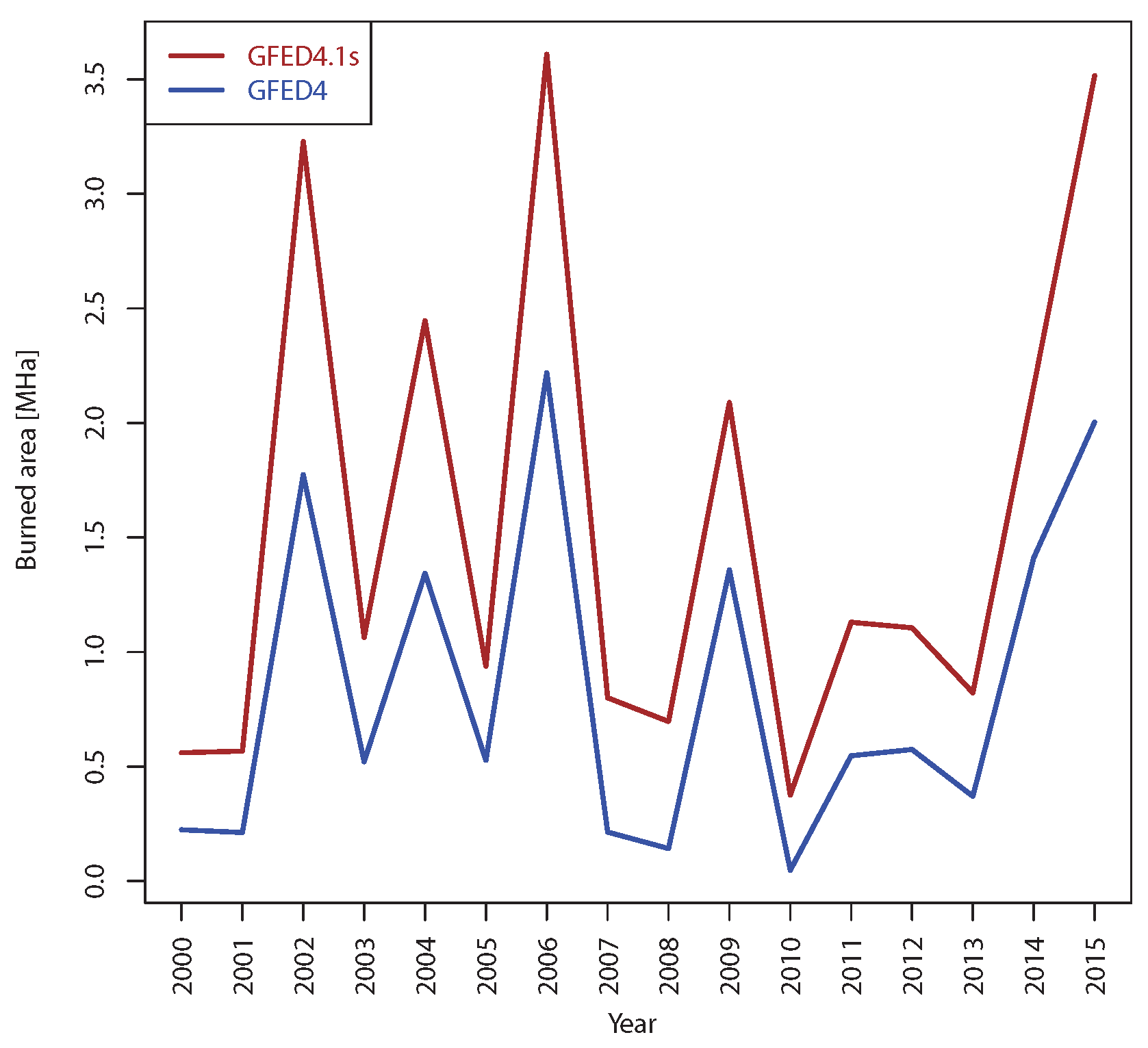
Currently, two versions of GFED are available: the one that includes small fires and another one that does not include them [53]; these are compared for Indonesia in Figure A1. One can see that small fires considerably increased the reported burned area, while the shape of the inter-annual variability stayed similar to the version without small fires. In this study, we use the version without small fires for the following reasons. Firstly, it includes the year 2016 (Version 4.1s is till 2015). Secondly, it contains information from the University of Maryland (UMD) land cover classification scheme applied to burned area and provides ratios of area burned in each of those classes, as well as the ratios of area burned in peatland. Note that GFED4.1s contains a split only for emissions. In our study, we model wildfires, and therefore, we choose burned area in the following 10 classes (out of 18): evergreen needleleaf forest, evergreen broadleaf forest, deciduous needleleaf forest, deciduous broadleaf forest, mixed forests, closed shrublands, open shrubland, woody savannas, savannas, grasslands [54]. Additionally, we use information on uncertainty intervals provided in GFED4, referred to as GFED in this paper.
A schematic illustration of how burned area is presented in GFED is shown in Figure 2a. Each grid cell contains information about total burned area. Additionally, we use the information of the fraction of area of wildfire (10 UMD land classes as mentioned above) and the fraction of area allocated to peat fire. Those fractions are independent, meaning that area burned by wildfire and peat fire can intersect in some areas, as indicated in the figure. Figure 2b shows actual data extracted for Indonesia from GFED separately for the total area burned, in wildland and peatland. The sum of areas burned in peatland and wildland is higher than the total burned area.
In our modeling, we use a similar approach. FLAM is calibrated separately for wildfire and peat fire, i.e., there are different suppression efficiencies. This approach allows us to distinguish between smoldering fires in peatland and flaming fires in forest.
2.6. Peatland Ratio Map
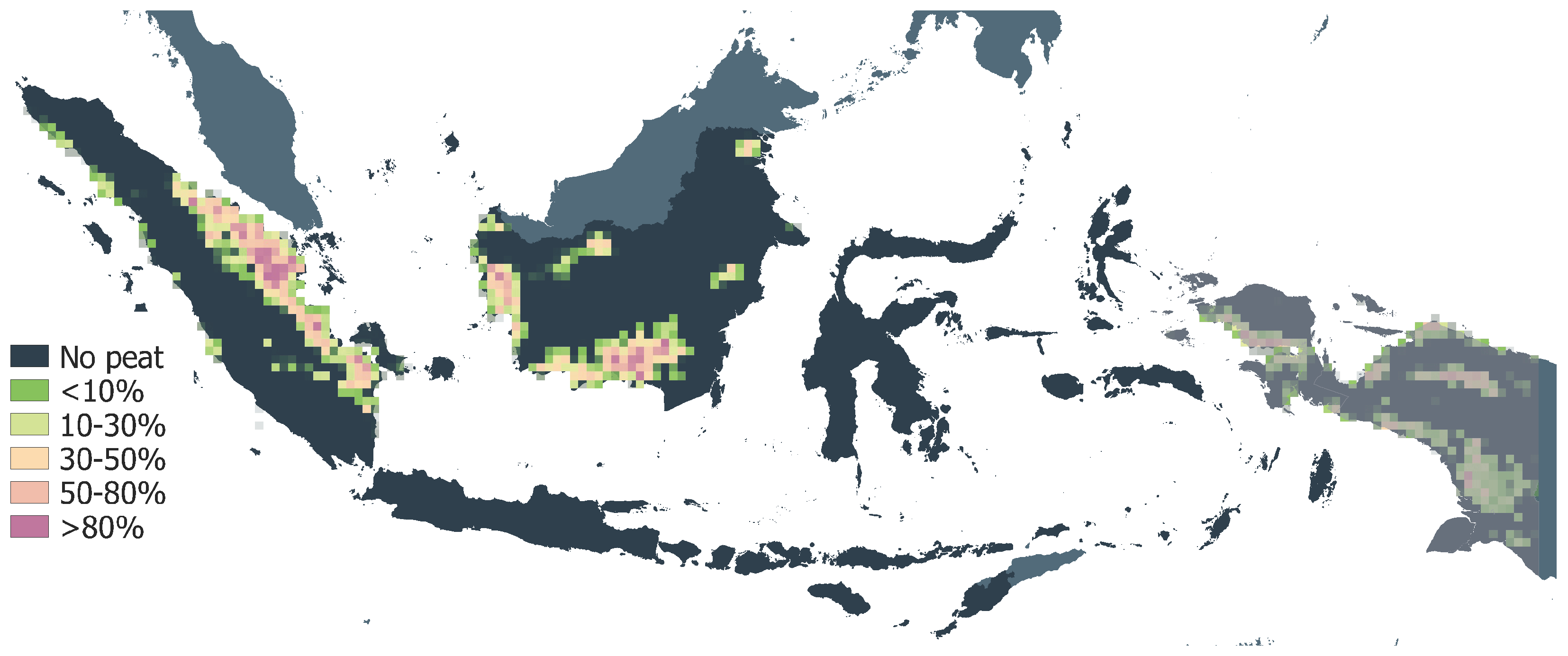
To calculate the fraction of area burned in peatland, we use a map produced by the Indonesian Ministry of Agriculture [55]. This map provides information on total share of peat in a grid cell in addition to burned peat within total burned area available in GFED. Original map indicated values of 1 for peat and 0 for no peat in each pixel at 30-m resolution. Based on these data, we calculated the ratio of peatland in each pixel at the 0.25-arc degree resolution as shown in Figure 3. The GFED dataset contains information on peat fires for Kalimantan and Sumatra. Therefore, in our analysis, we use the peatland map only for these islands. Nevertheless, we show the entire map with Papua greyed out.
3. Results
In this section we present the results of the FLAM model applied to Indonesia in their temporal and spatial dimensions. This is comprised of results for the model calibration and validation.
3.1. Temporal Validation of FLAM Modeling Results
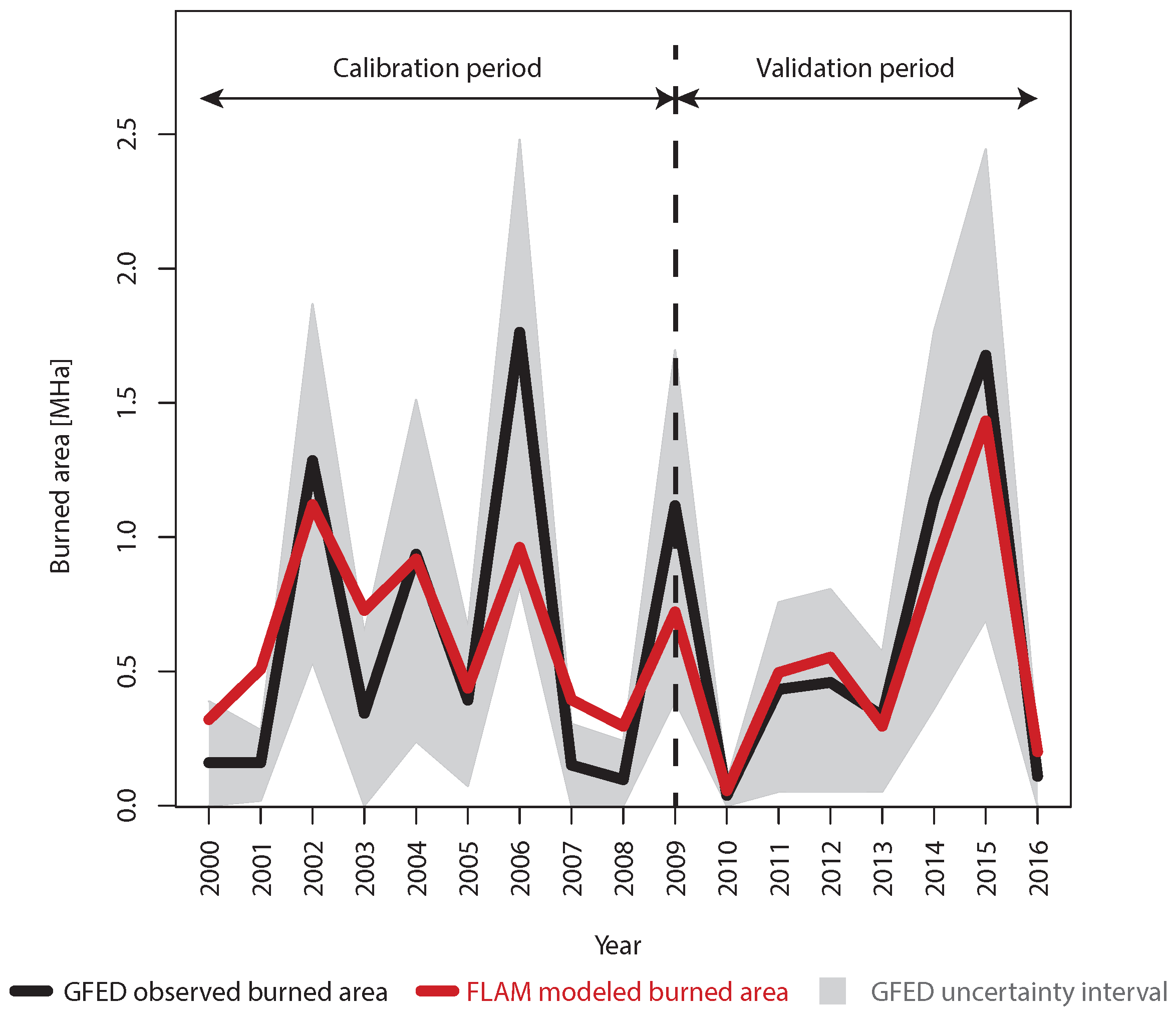
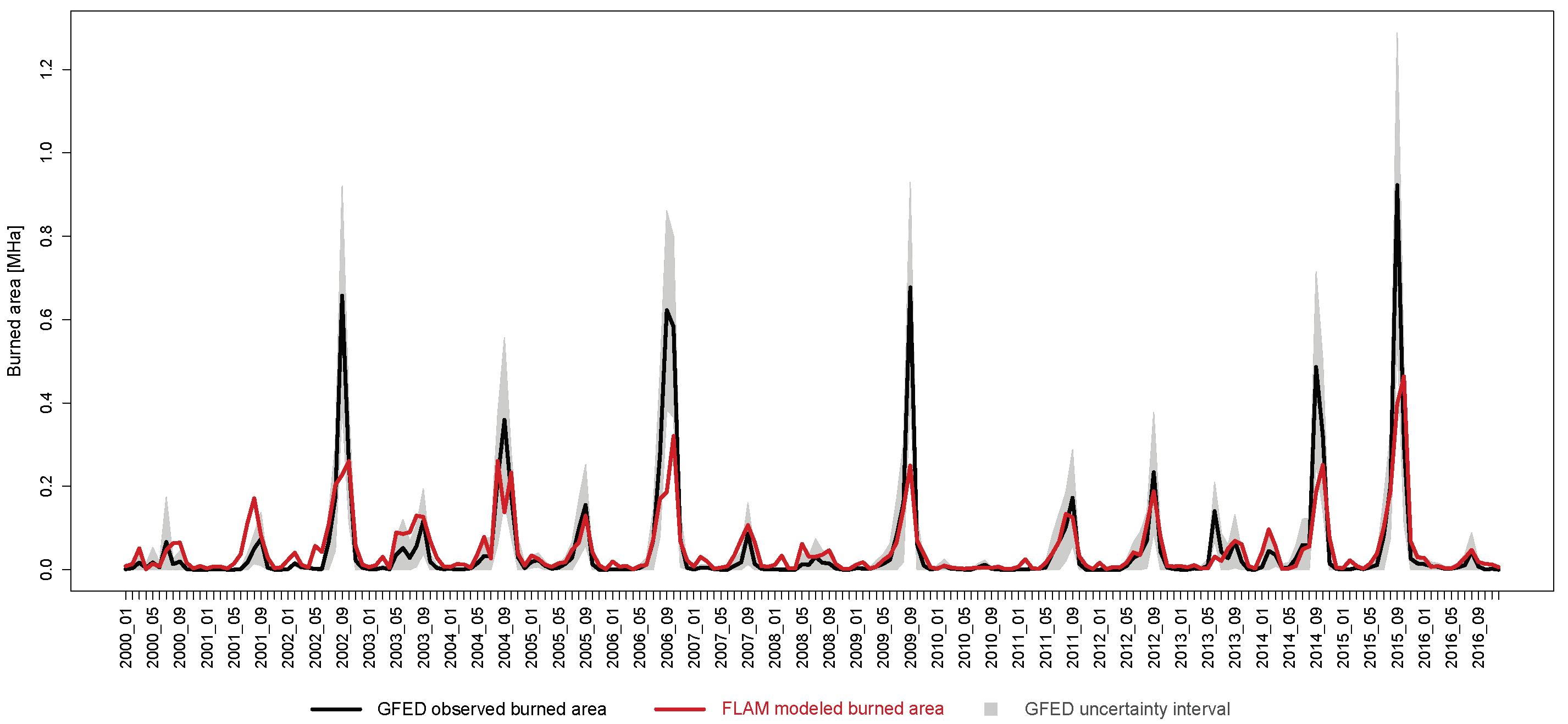
Figure 4 shows the fit of annual burned area during wildfires over the entirety of Indonesia. In the calibration period, observed burned area in GFED (black line), accumulated from 2000–2009, was used for FLAM calibration (see Section 2.4). In the period 2010–2016, annual GFED data were used for validation of the burned area estimated by FLAM (red line). The figure demonstrates that FLAM fit actual observations quite well. The red line follows the black line and usually is in the range of indicative uncertainty intervals of GFED. Here, we used burned area uncertainty (in ha) reported in GFED [29].
We compared burned areas modeled by FLAM and reported by GFED using two indicators: Pearson’s correlation coefficient (r) and Mean Absolute Error (MAE). The corresponding values of MAE and Pearson’s r are provided in Table 1 separately for calibration and validation periods. For the validation period, we obtained very high values of Pearson’s , both for wildfires and peat fires. MAE values were 106.71 and 35.56 thousands hectares, respectively, for wild- and peat fires (19% and 11% relative to the average annual burned area). Lower values of Pearson’s r, 0.857 and 0.865, respectively, were obtained in the calibration period, which can be explained by the extreme fires in 2006 reported by GFED, but not entirely captured by FLAM (see Figure 4 and Figure 5). This could also explain the higher values of MAE in the calibration period compared to the validation period. The ability to capture large fires in 2015 by FLAM in the validation period was high. Here, no information from GFED was used, and the model was running only with updated input data in the period 2010–2016.
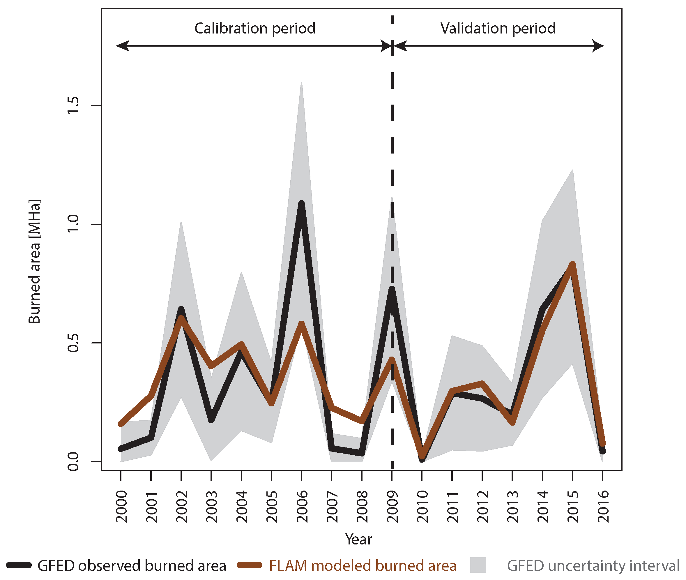
In order to compare modeled areas burned by peat fires with the data reported by GFED, we used the peatland mask as described in Section 2.6. The corresponding dynamics of burned area in peatland of Sumatra and Kalimantan is shown in Figure 5. Accumulated burned areas for Figure 4 and Figure 5 can be found in Table 4 below.
3.2. Analysis of the Calibrated Suppression Efficiency Maps
Here, we present detailed results of the calibration procedure (see Section 2.4) that was applied in the validation period. The suppression efficiency maps were obtained using GFED observations, accumulated over 2000–2009, separately for wildfires and peat fires. These maps were used by FLAM for estimation of the spatial and temporal dynamics of burned area in the calibration and validation periods.
3.2.1. Spatial Distribution of Suppression Efficiency for Wildfire
During the calibration procedure, 6% of area in GFED burned in pixels that could not be calibrated in FLAM due to the absence of climate data (see Section 2.4.3). The problem was that the country mask used in the climatic data of GWFED did not coincide with the country mask used by GFED (see Figure A2). For this reason, we excluded those pixels (where climate data were not available) from the analysis. We removed from our consideration about 1% of pixels marked as having any burned area in GFED (totaling about 1% of all burned area), where FLAM was not able to reproduce any fire due to various reasons (e.g., no fuel, no ignition source).
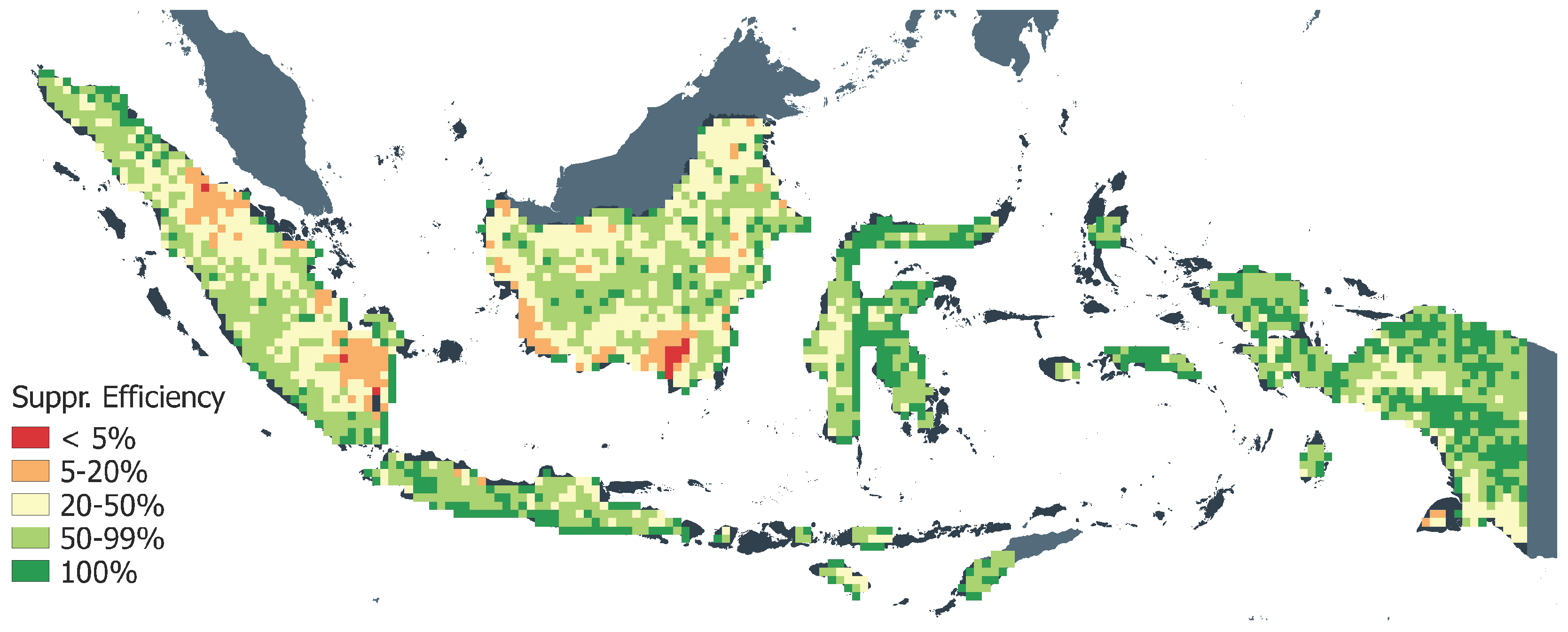
Figure 6 shows how calibrated suppression efficiency varies across Indonesia. Areas with high values of parameter are colored in green. The dark green color is attached to pixels with , where fire occurrence was excluded by the calibration procedure (see Section 2.4.1). Statistical analysis of ratios of pixels with various thresholds for suppression efficiency, as well as the ratio of accumulated area burned in those pixels are provided in Table 2. We also present the ratio of accumulated burned area in the same pixels for the original fire algorithm without the application of the calibration procedure and with the fixed parameter for the entirety of Indonesia. Note that 0.5 was also the smallest value in the study by Arora and Melton [28]. Actually, there was a substantial amount of pixels in diapason , i.e., 42% of all pixels. However, only 5% of the total burned area was attributed to these pixels (both in GFED and FLAM) versus 35% in the original algorithm. Note that as FLAM was calibrated using accumulated GFED, their accumulated areas coincided in the calibration period in each pixel, while there was annual variability in burned areas driven by FLAM inputs. The original algorithm models 46% of area burned in pixels, where , meaning that in fact, according to GFED, there were no fires in those pixels (0% of area burned in FLAM). This illustrates a considerable improvement in spatial accuracy by application of the calibration procedure realized in this study.
Note that according to Table 2, 95% of area burned in pixels where , and 63% of area burned in pixels where (orange and red areas in Figure 6). This analysis shows that considerable area burned in a small amount of pixels with a very low suppression efficiency. For instance, 35% of area burned in 2% of pixels within threshold . Figure 3 and Figure 6 show that pixels with low suppression efficiency were mostly located in peatland areas. The pixel with the lowest value of is located in Borneo swamp forest. According to Equation (12), this value corresponds to the average fire duration of 47 days.
3.2.2. Spatial Distribution of Suppression Efficiency for Peat Fire
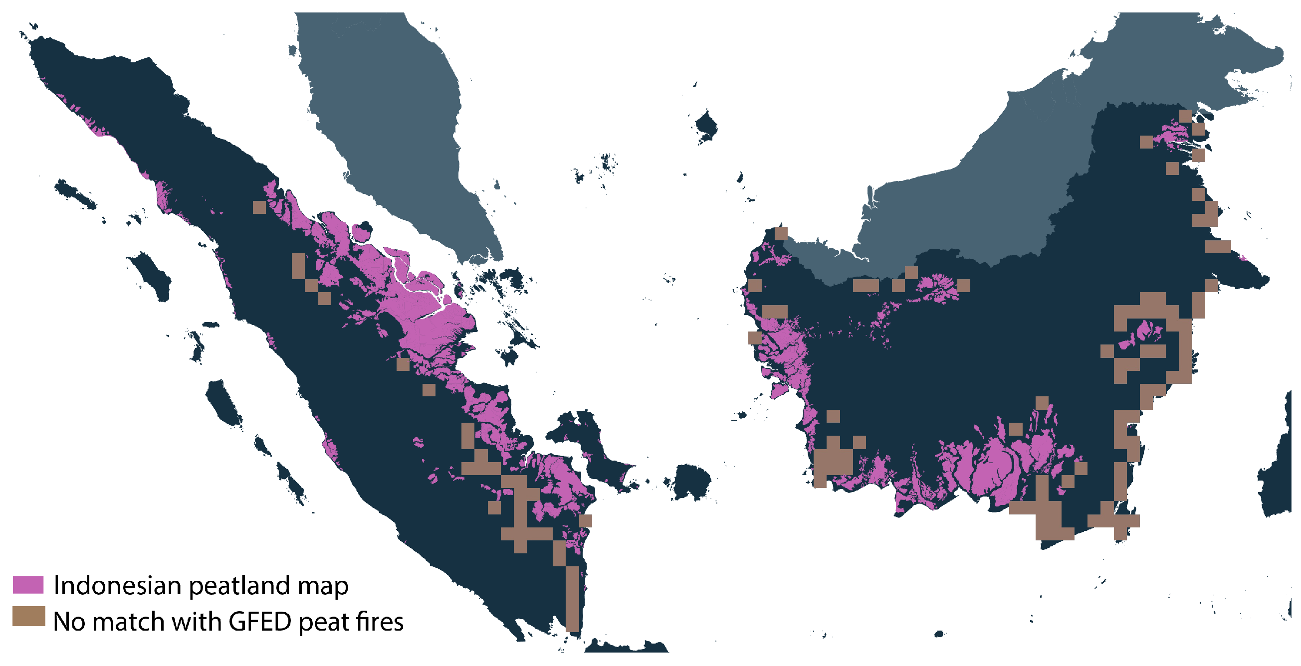
During the calibration procedure, we found out that 20% of area burned in peatland in GFED was located in pixels where there were no peat fires according to FLAM. This can be explained by the difference in peatland masks used in GFED and FLAM. It seems that GFED allocated peatland to a wider class of land than actual peatland. Our understanding from the publication describing GFED [54] is that the Terrestrial Ecosystems of the World map [56] was used as the source for peatland data. It seems that all types of swamp forests according to the map were considered as peatland. For this reason, we removed those pixels, which were outside of the peatland mask (see Section 2.6) in our analysis, from the GFED data (see Figure A3). We removed from our consideration about 1% of pixels marked as having any burned area in GFED (totaling about 1% of all burned area), where FLAM was not able to reproduce any fire due to various reasons (e.g., no fuel, no ignition source).
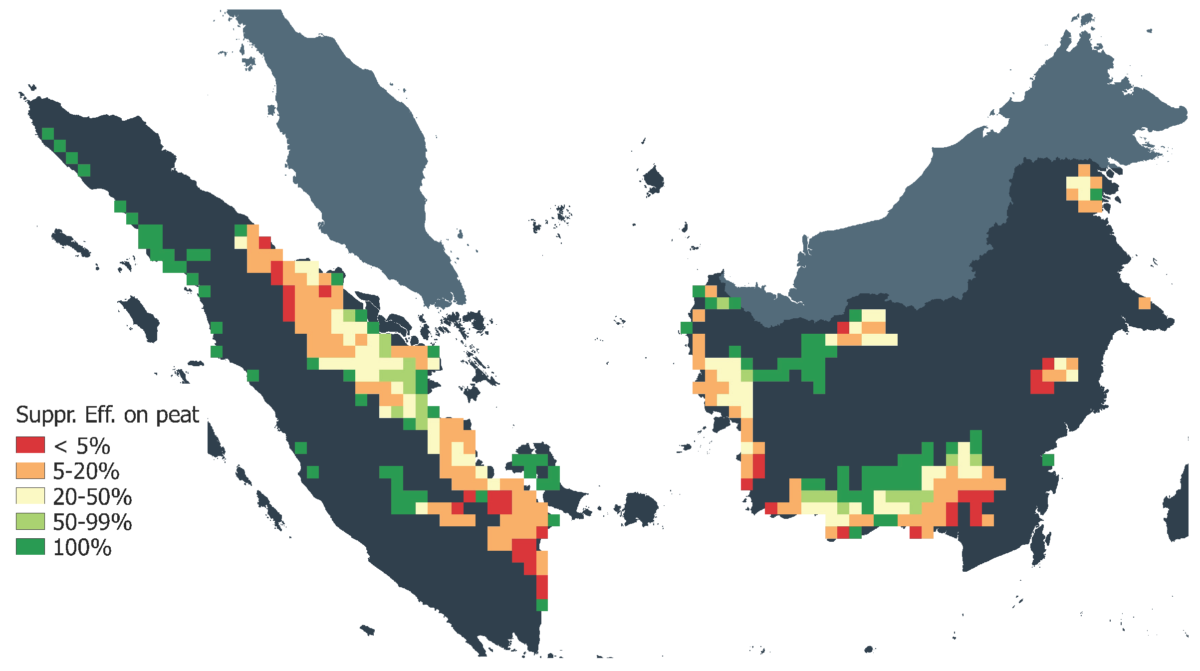
Spatial distribution of suppression efficiency in peatland is shown in Figure 7. Again, we outline the pixels, where the probability of extinguishing a fire equals one. The statistics of pixels with various thresholds for in peatland, as well as information for corresponding areas burned in FLAM and the original algorithm are given in Table 3. Interestingly, 94% of area burned in pixels with very low suppression efficiency, i.e., . The minimum value of was 0.00574, which according to Equation (12), corresponds to the average duration of 173 days. This reflects the actual situation in Southeast Asia, where once established, peat fires may burn for months and are very difficult to control; in particular, when they occur in remote, off-road locations where they are difficult to extinguish using conventional fire-fighting techniques [57].
Identifying pixels with very low suppression efficiency, FLAM is able to capture the phenomena of smoldering fires, the most difficult types of fires to extinguish [58]. Comparing Figure 7 for peat fire and Figure 6 for wildfire, one can see that the areas with low suppression efficiency (red and orange colored areas) often coincide. This observation may indicate possible transition from flaming fires (in forest) to smoldering fires (in peatland). The opposite direction, from smoldering to flaming fires, could also happen in rare cases [58].
3.2.3. Bimodal Density Functions of Suppression Efficiency
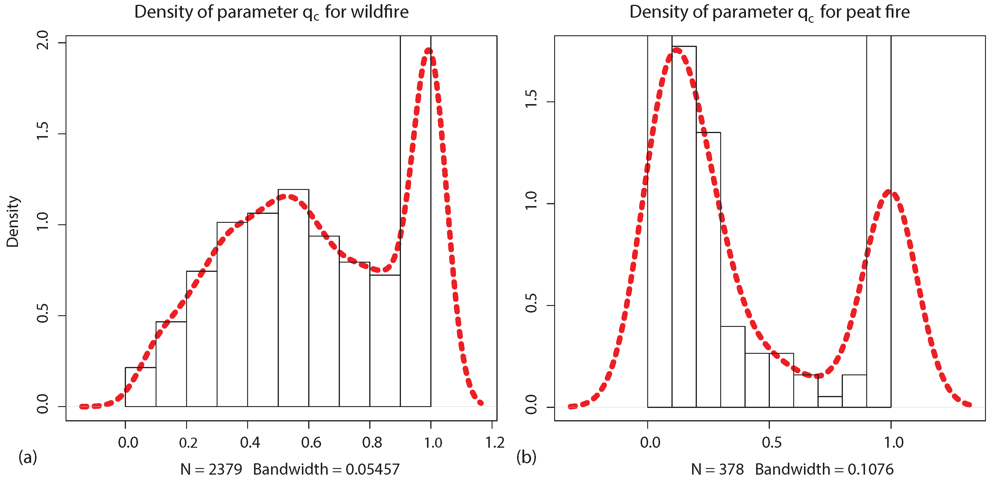
To summarize the previous sub-subsection, we have produced histograms and smoothing density functions in R for calibrated suppression efficiency maps. They are presented in Figure 8 for (a) wildfire and (b) peat fire. Both distributions have a bimodal shape, which shows that calibration procedure corrects the areas estimated by the original algorithm in both directions. It removes the areas where the fires could not occur according to observations. Where the observed areas are underestimated, suppression efficiency is adjusted to lower values.
Although mean values of the density functions in Figure 8 (0.64 for wildfire and 0.42 for peat fire) are close to 0.5 (the minimum value in [28]), our analysis above shows that most of the area burned in pixels with very low suppression efficiency. Lower suppression efficiency corresponds to longer fire duration. According to our calibration procedure (see Table 2 and Table 3) and Equation (12), for wildfires, 63% of area burned in pixels where the average duration of fire was more than four days, and in peatland, 77% of area burned in pixels with an average fire duration of more than nine days.
3.3. FLAM vs. Original Fire Algorithm
Finally, we show how the calibration of suppression efficiency improves the agreement between modeled and observed total burned areas, as well as the ratio of peat fire to wildfire in FLAM, as compared to the original fire algorithm. Table 4 shows the corresponding burned areas for two periods for GFED, FLAM and the original fire algorithm ( uniformly). In the calibration period, accumulated GFED and FLAM areas coincided due to the calibration procedure (see Section 2.4). Note, that inter-annual dynamics of burned area was not forced to coincide and was driven by FLAM inputs (mostly weather) in the calibration and validation periods (see Figure 4 and Figure 5). The ratio of peat fire to wildfire was 59% in the calibration period. The original algorithm underestimated burned area by wildfire reported in GFED by around 2.74 million ha and very significantly underestimated area burned in peatland (only 0.12 vs. 3.59 mln.ha). This led to an unrealistic ratio of 4% of peat to wildfire areas. This is another illustration of how much the calibration procedure proposed in FLAM improves model performance compared to using a fixed value of .
Moreover, Table 4 shows that in the validation period, where areas estimated by FLAM and observed by GFED did not necessary coincide, FLAM kept good track of GFED observations. In particular, total areas burned in peatland were almost the same and in wildland were very close. This demonstrates a good temporal fit as reported in previous Section 3.1 for the validation period. Table 4 indicates that the original fire algorithm considerably underestimated burned area in the validation period similar to the calibration period.
3.4. Spatial Validation of Estimated Burned Area
Here, we present the results of the spatial validation of the estimated burned area for the period 2010–2016. We calculated Pearson’s correlation coefficients r based on annual dynamics of burned area (in GFED and FLAM) in each grid cell separately for wildfires and fires in peatland.
3.4.1. Spatial Correlation for Peat Fire
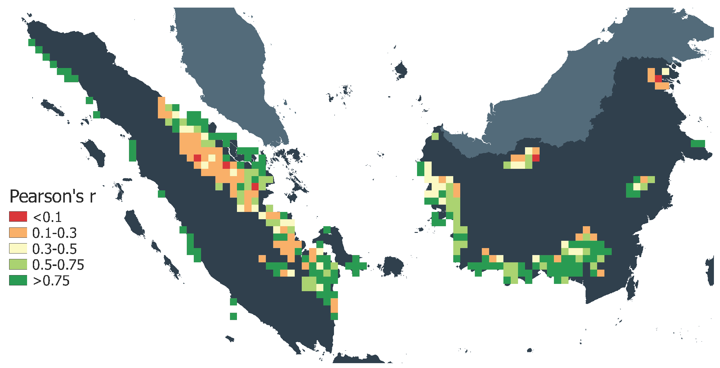
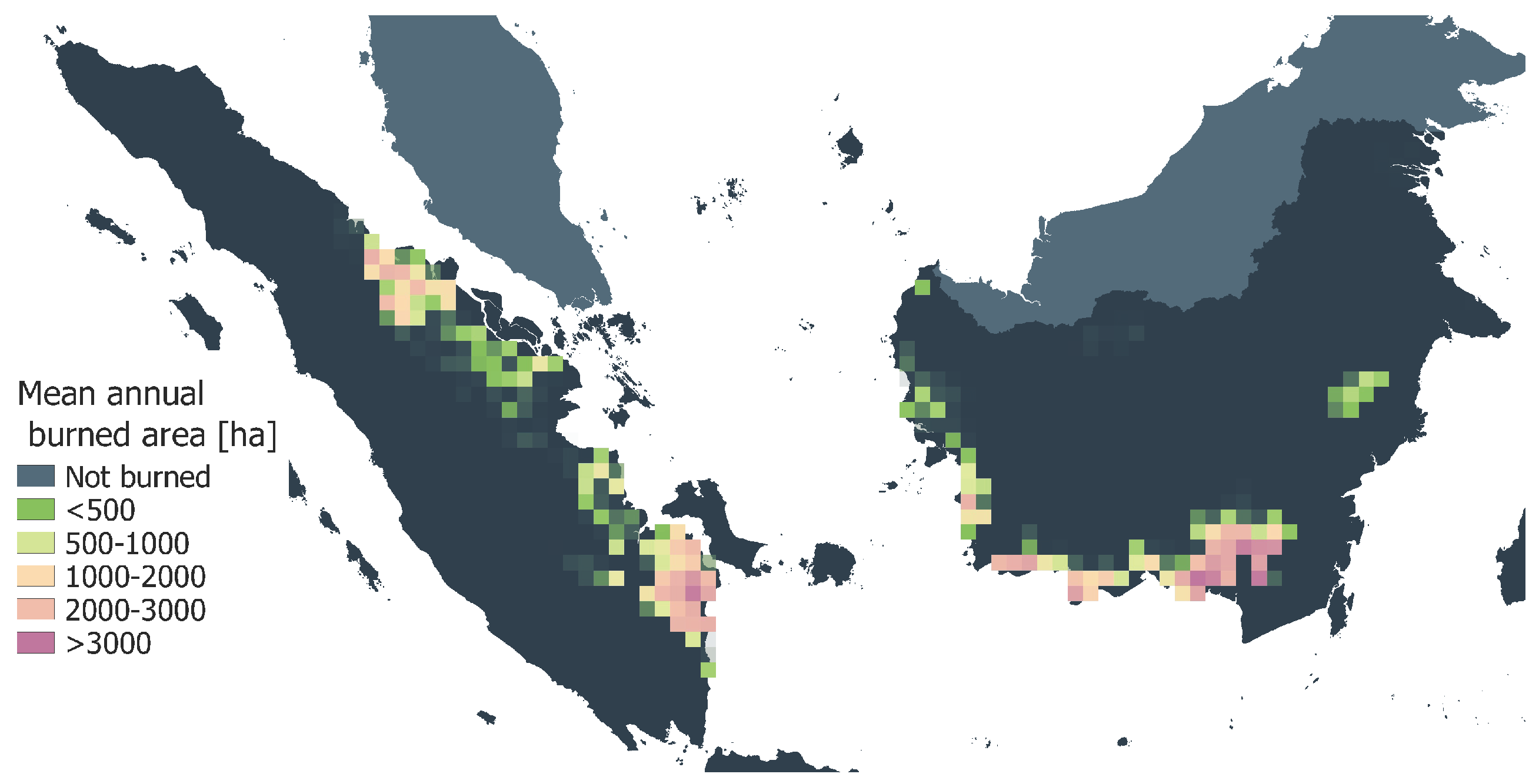
Results in Table 5 show the ratio of pixels with various correlation thresholds, as well as the ratio of aggregated burned area with respect to burned area in all pixels in FLAM and GFED, respectively. One can see that positive values of Pearson’s r were achieved in 90% of pixels, and at the same time, 98% of area was burned in these pixels during the entire time interval (2010–2016). In pixels where 75% of total area was burned in GFED, the correlation is above 0.6. Figure 9 shows the distribution of Pearson’s r across peatland area, and Figure 10 shows the mean annual burned area in each pixel. Comparing those figures, we see that higher correlation coefficients (green-colored pixels in Figure 9) often corresponded to the area where there was high burned area values (purple pixels in Figure 10). At the same time, pixels with a low correlation (orange and red in Figure 9) often coincided with pixels where burned area was relatively small.
3.4.2. Spatial Correlation for Wildfire
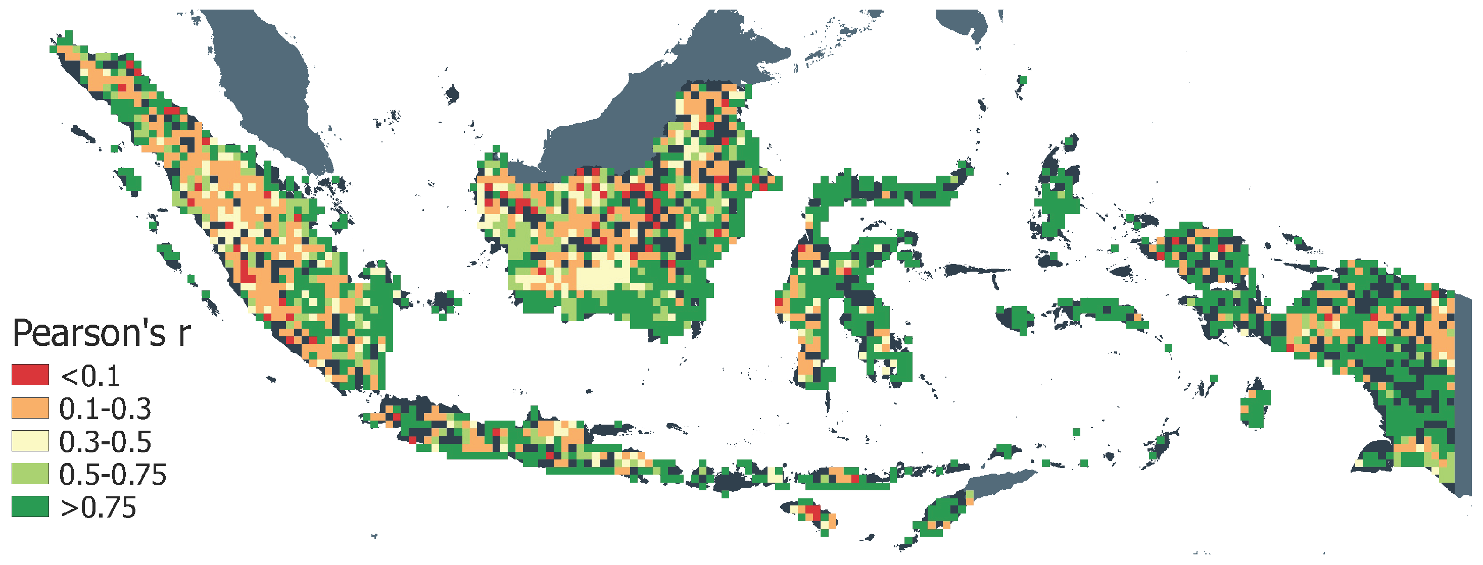
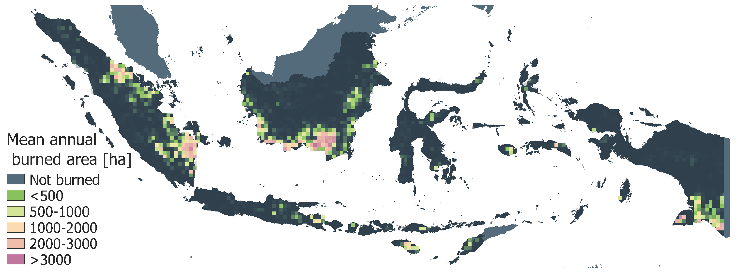
Similar to burned area in peatland, we present correlation results for wildfire. As follows from Table 6, in pixels where 76% of area burned, the Pearson’s correlation coefficient was above 0.5. Remarkably in 40% of pixels, the correlation was above 0.9. We present the spatial distribution of Pearson’s r in wildfires in Figure 11 and mean annual burned area in GFED in Figure 12. They show that a high correlation was achieved in areas with large fires, i.e., in Sumatra and Kalimantan, while lower correlation coefficients were often in the areas with relatively small fires.
4. Discussion
In this study, we applied FLAM to the assessment of burned areas in Indonesia. The model was calibrated in the 10-year period (2000–2009) and validated over the seven-year period (2010–2016) using GFED observed burned area. In order to check how results would change with respect to different calibration/validation periods, we considered an alternative split of the historical period into two intervals: seven years for calibration (2000–2006) and 10 years for validation (2007–2016). The corresponding modeling results are given in Table A1. The results show that because of a shorter calibration period, the values of the Pearson’s r are lower compared to those in Table 1. Nevertheless, the correlation with GFED is still very good in the extended validation period (2007–2016): 0.914 for peat fire and 0.956 for wildfire. The corresponding MAE values are 87.65 and 154.9 thousands ha (38% and 36% with respect to average annual burned area). This increase in MAE compared to that of the 10-year calibration period is due to the fact that years 2007–2009, where FLAM is challenged in reproducing burned areas, are now included in the validation period. Experiments with shorter calibration periods provide a decrease in Pearson’s r in validation periods as the model requires sufficient number of years with “peaks” (2002, 2004, 2006) for calibration. In our view, the 10-year calibration period is sufficient for calibrating FLAM.
Calibration of the spatial suppression efficiency performed in this study provides an important development in the methodology of the application of the original Arora and Boer [27] algorithm. Our findings show that the distribution of suppression efficiency has a bimodal density function. A recent publication [28] applying the same core algorithm by Arora and Boer [27] for fire modeling states that in the absence of any human influence, the probability of extinguishing a fire within one day equals 0.5 and corresponds to an average fire duration of one day; the extinguishing probability increases with population density. We show that this global value is unrealistic for tropical forests using the example of Indonesia. The results of model calibration using historical GFED data [29] show that in Indonesia, 95% of area burned by wildfire is located in pixels where the extinguishing probability is below 0.5. It could be as low as 0.0057 in the peatland of the Borneo swamp forest, where the Mega Rice project [59] took place, corresponding to an average fire duration of 173 days. This reflects the actual situation in Southeast Asia, where once established, peat fires may burn for months and are very difficult to extinguish [57]. We show that the application of the algorithm without calibration considerably underestimated burned area, particularly in peatland. Our conclusion is that the approach proposed by Arora and Melton [28] may help to fit a decreasing trend in global burned area, but at the price of considerably underestimating regional burned area, e.g., in Indonesia, which produces a great deal of global CO emissions. Underestimation of burned area by the original fire algorithm with could also be the reason why the majority of global fire models underestimate the global burned area, as reported in the study led by Andela [52].
Validation results on a pixel scale show that in pixels where around 70% of area is burned, the correlation coefficients are above 0.6 and in those where around 30% of area is burned, above 0.9, both for peat and wildfire. We show figures for the spatial distribution of correlation coefficients and compare them with the maps of mean annual burned area. The comparison of maps shows that high correlation is often achieved in the pixels with a large burned area, mostly located in the peatland of Sumatra and Kalimantan. At the same time, lower correlation coefficients are often in the pixels with small burned area. Capturing pixels with small fires could be a potential direction for spatial improvement of FLAM modeling, where the GFED version with small fires can be used [53].
We would like to emphasize that the simplified approach used for modeling peat fires produced good results. It is also interesting to mention that areas with large wildfires and peat fires often coincide. Our analysis of the spatial variability of the suppression efficiency for wildfires and peat fires can potentially allow one to find the areas where smoldering and flaming fires are tightly related [58]. However, further analysis has to be carried out in this direction.
FLAM was able to correctly estimate extreme burned area in 2015, which caused a lot of damage in Indonesia [9]. While the calibration procedure uses only accumulated burned area from GFED, the good inter-annual variability is due to adequate representation of daily weather dynamics in FLAM. An interesting observation is that FLAM was not able to capture 2006 in the calibration period. This could indicate an uncertainty in the GFED dataset, bias in climate data or an increase of ignition potential, e.g., due to human activity. Finally, we explored the fire dynamics at a finer temporal scale and showed a comparison of monthly dynamics between GFED and FLAM areas burned by wildfires in Figure A4. Preliminary analysis based on the figure shows that FLAM is not always capturing the highest burned area in September. Potentially, seasonal calibration of the suppression efficiency could lead to the improvement of FLAM monthly estimates, and consequently better spatial and temporal results. A promising direction for future research would be the assessment of greenhouse gases emissions based on burned areas modeled by FLAM.
Current peat fires and wildfires can affect future fires in two main areas. On the non-anthropogenic side, current fires will highly affect soil moisture and the water content of biomass. This will increase the likelihood of fire occurrence within a relatively short period until adequate rainfall compensates the loss of soil moisture and water content. From the anthropogenic perspective, physical alteration of the environment such as canal drainage in peat areas or land clearance for crop production can have an effect. If no restoration activities are carried out, peat fire is likely to reoccur.
5. Conclusions
In this study, we applied FLAM to estimate burned area in Indonesia and validated these results independently of the model calibration for the first time. For burned areas aggregated over Indonesia, we obtained Pearson’s correlation coefficient separately for wildfires and peat fires, which turns out to be equal to 0.988 in both cases. Spatial correlation analysis showed that in pixels where around 70% of area is burned, the correlation coefficients are above 0.6, and in those, where 30% of area is burned, above 0.9. We showed that FLAM is capable of capturing not only flaming, but also smoldering peat fires, which are crucially important for Indonesia.
The suggested approach for the spatial calibration of the probability of extinguishing a fire improves the results of the original Arora and Boer fire algorithm. We showed that the calibrated parameter has a bimodal distribution over Indonesia; in areas where the probability is found to be close to one, the fire occurrence could be diminished due to human activity; at the same time, in areas where this parameter is found to be close to zero, human activity, on the contrary, leads to extensive fire, for example due to slash and burn agriculture or peatland drainage. Very low suppression levels are found in the peatland of Kalimantan and Sumatra, where fire can burn for very long periods of time despite extensive rains, weather changes and fire-fighting attempts.
The results presented in this paper are a prerequisite for estimating future burned area under projected climate change and for modeling adaptation options. Modeling burned area in Indonesia and an assessment of corresponding impacts, e.g., CO emissions, can be potentially used for climate/economic damage assessments. This could also help to adequately represent the risks of wildland fires in REDD+ programs [60,61]. Modeling fire ignition and suppression can also help the implementation of fire prevention policies and provide important information for building adequate and cost-efficient fire response infrastructure.
Author Contributions
A.K., N.K., J.P., F.K., P.Y., D.S. and M.O. designed the study. A.K. and N.K. coded the FLAM model. A.K. performed the FLAM runs, calibration and validation. A.K., J.P. and D.S. preprocessed the data. J.P. prepared the maps. A.K., N.K., J.P. and P.Y. wrote the paper.
Funding
This work was supported by the RESTORE+project (www.restoreplus.org), which is part of the International Climate Initiative (IKI), supported by the Federal Ministry for the Environment, Nature Conservation and Nuclear Safety (BMU) based on a decision adopted by the German Bundestag. It received support from the project ”Delivering Incentives to End Deforestation: Global Ambition, Private/Public Finance, and Zero-Deforestation Supply Chains” funded by the Norwegian Agency for Development Cooperation under Agreement Number QZA-0464 QZA-16/0218. Furthermore, the work has been funded by IIASA’s Tropical Futures Initiative (TFI).
Acknowledgments
We would like to thank Sandy Harrison, Anatoly Shvidenko, Daniel Murdiyarso and Sergey Venevsky for valuable comments and suggestions.
Conflicts of Interest
The authors declare no conflict of interest. The founding sponsors had no role in the design of the study; in the collection, analyses or interpretation of data; in the writing of the manuscript; nor in the decision to publish the results.
Abbreviations
The following abbreviations are used in this manuscript:
| FLAM | wildFire cLimate impacts and Adaptation Model |
| GFED | Global Fire Emissions Database |
| MODIS | Moderate Resolution Imaging Spectroradiometer |
| SFM | Standalone Fire Model |
| FWI | Fire Weather Index |
| DGVM | Dynamic Global Vegetation Model |
| FFMC | Fine Fuel Moisture Code |
| GPW | Gridded Population of the World |
| HRMC | High Resolution Monthly Climatology |
| OTD | Optical Transient Detector |
| LIS | Lightning Imaging Sensor |
| TRMM | Tropical Rainfall Measuring Mission |
| ABG | Above-Ground Biomass |
| CWD | Coarse Woody Debris |
| GFWED | Global Fire WEather Database |
| MERRA | Modern Era Retrospective Analysis for Research and Applications |
| NASA | National Aeronautics and Space Administration |
| REDD | Reduce Emissions from Deforestation and Forest Degradation |
Appendix A. Supplementary Figures
Figure A1.
Annual dynamics of total burned area, extracted for Indonesia from two versions of GFED: GFED4 and GFED4.1s. The addition of small fires considerably increased the reported burned area.
Figure A1.
Annual dynamics of total burned area, extracted for Indonesia from two versions of GFED: GFED4 and GFED4.1s. The addition of small fires considerably increased the reported burned area.

Figure A2.
Pixels (orange) with positive burned area reported by GFED for the calibration period (2000–2009), where FLAM does not model burned area due to the missing climate data.
Figure A2.
Pixels (orange) with positive burned area reported by GFED for the calibration period (2000–2009), where FLAM does not model burned area due to the missing climate data.

Figure A3.
Pixels with positive burned area reported by GFED for the calibration period (2000–2009) in peatland, which are located outside of the peatland map used in the study.
Figure A3.
Pixels with positive burned area reported by GFED for the calibration period (2000–2009) in peatland, which are located outside of the peatland map used in the study.

Figure A4.
Monthly dynamics of area burned by wildfires.


Table A1.
Mean absolute error (MAE) and Pearson’s r for annual country level burned areas reported in GFED and modeled in FLAM for the calibration period 2000–2006 and the validation period 2007–2016.
Table A1.
Mean absolute error (MAE) and Pearson’s r for annual country level burned areas reported in GFED and modeled in FLAM for the calibration period 2000–2006 and the validation period 2007–2016.
| Period | Calibration Period (2000–2006) | Validation Period (2007–2016) | ||
|---|---|---|---|---|
| Type of Fire | Peat Fire | Wildfire | Peat Fire | Wildfire |
| Pearson’s r | 0.838 | 0.85 | 0.914 | 0.956 |
| MAE (thousands of ha) | 155.7 | 257.51 | 87.65 | 154.9 |
| MAE relative to average burned area | 46% | 43% | 38% | 36% |
References
- Bowman, D.M.; Balch, J.K.; Artaxo, P.; Bond, W.J.; Carlson, J.M.; Cochrane, M.A.; D’Antonio, C.M.; DeFries, R.S.; Doyle, J.C.; Harrison, S.P.; et al. Fire in the Earth system. Science 2009, 324, 481–484. [Google Scholar] [CrossRef] [PubMed]
- Marlier, M.E.; DeFries, R.S.; Voulgarakis, A.; Kinney, P.L.; Randerson, J.T.; Shindell, D.T.; Chen, Y.; Faluvegi, G. El Niño and health risks from landscape fire emissions in southeast Asia. Nat. Clim. Chang. 2013, 3, 131. [Google Scholar] [CrossRef] [PubMed]
- Jolly, W.M.; Cochrane, M.A.; Freeborn, P.H.; Holden, Z.A.; Brown, T.J.; Williamson, G.J.; Bowman, D.M. Climate-induced variations in global wildfire danger from 1979 to 2013. Nat. Commun. 2015, 6, 7537. [Google Scholar] [CrossRef] [PubMed] [Green Version]
- Flannigan, M.; Cantin, A.S.; De Groot, W.J.; Wotton, M.; Newbery, A.; Gowman, L.M. Global wildland fire season severity in the 21st century. For. Ecol. Manag. 2013, 294, 54–61. [Google Scholar] [CrossRef]
- Bowman, D.M.; Williamson, G.J.; Abatzoglou, J.T.; Kolden, C.A.; Cochrane, M.A.; Smith, A.M. Human exposure and sensitivity to globally extreme wildfire events. Nat. Ecol. Evol. 2017, 1, 0058. [Google Scholar] [CrossRef] [PubMed]
- San-Miguel-Ayanz, J.; Moreno, J.M.; Camia, A. Analysis of large fires in European Mediterranean landscapes: lessons learned and perspectives. For. Ecol. Manag. 2013, 294, 11–22. [Google Scholar] [CrossRef]
- Shvidenko, A.; Schepaschenko, D. Climate change and wildfires in Russia. Contemp. Probl. Ecol. 2013, 6, 683–692. [Google Scholar] [CrossRef]
- Herawati, H.; Santoso, H. Tropical forest susceptibility to and risk of fire under changing climate: A review of fire nature, policy and institutions in Indonesia. For. Policy Econ. 2011, 13, 227–233. [Google Scholar] [CrossRef]
- World Bank. The Cost of Fire: An Economic Analysis of Indonesia’s 2015 Fire Crisis; Technical Report, Indonesia Sustainable Landscapes Knowledge; note no. 1.; World Bank Group: Washington, DC, USA, 2016. [Google Scholar]
- Nurhidayah, L.; Djalante, R. Examining the Adequacy of Legal and Institutional Frameworks of Land and Forest Fire Management from National to Community Levels in Indonesia. In Disaster Risk Reduction in Indonesia; Springer: Cham, Switzerland, 2017; pp. 157–187. [Google Scholar]
- Page, S.E.; Rieley, J.O.; Banks, C.J. Global and regional importance of the tropical peatland carbon pool. Glob. Chang. Biol. 2011, 17, 798–818. [Google Scholar] [CrossRef] [Green Version]
- Hooijer, A.; Page, S.; Canadell, J.; Silvius, M.; Kwadijk, J.; Wösten, H.; Jauhiainen, J. Current and future CO2 emissions from drained peatlands in Southeast Asia. Biogeosciences 2010, 7, 1505–1514. [Google Scholar] [CrossRef]
- Rieley, J.; Page, S. Tropical Peatland of the World. In Tropical Peatland Ecosystems; Springer: Tokyo, Japan, 2016; pp. 3–32. [Google Scholar]
- Page, S.E.; Siegert, F.; Rieley, J.O.; Boehm, H.D.V.; Jaya, A.; Limin, S. The amount of carbon released from peat and forest fires in Indonesia during 1997. Nature 2002, 420, 61. [Google Scholar] [CrossRef] [PubMed]
- Harrison, M.E.; Page, S.E.; Limin, S.H. The global impact of Indonesian forest fires. Biologist 2009, 56, 156–163. [Google Scholar]
- Tacconi, L. Fires in Indonesia: Causes, Costs and Policy Implications; Technical Report; CIFOR: Bogor, Indonesia, 2003. [Google Scholar]
- Field, R.D.; van der Werf, G.R.; Fanin, T.; Fetzer, E.J.; Fuller, R.; Jethva, H.; Levy, R.; Livesey, N.J.; Luo, M.; Torres, O.; et al. Indonesian fire activity and smoke pollution in 2015 show persistent nonlinear sensitivity to El Niño-induced drought. Proc. Natl. Acad. Sci. USA 2016, 113, 9204–9209. [Google Scholar] [CrossRef] [PubMed]
- Murdiyarso, D.; Lebel, L. Local to global perspectives on forest and land fires in Southeast Asia. Mitig. Adapt. Strat. Glob. Chang. 2007, 12, 3–11. [Google Scholar] [CrossRef]
- Albar, I.; Jaya, I.N.S.; Saharjo, B.H.; Kuncahyo, B. Spatio-Temporal Typology of Land and Forest Fire in Sumatra. Ind. J. Electr. Eng. Comput. Sci. 2016, 4, 83–90. [Google Scholar] [CrossRef]
- Herawati, H.; González-Olabarria, J.R.; Wijaya, A.; Martius, C.; Purnomo, H.; Andriani, R. Tools for assessing the impacts of climate variability and change on wildfire regimes in forests. Forests 2015, 6, 1476–1499. [Google Scholar] [CrossRef]
- Dutta, R.; Aryal, J.; Das, A.; Kirkpatrick, J.B. Deep cognitive imaging systems enable estimation of continental-scale fire incidence from climate data. Sci. Rep. 2013, 3, 3188. [Google Scholar] [CrossRef] [PubMed]
- Dutta, R.; Das, A.; Aryal, J. Big data integration shows Australian bush-fire frequency is increasing significantly. R. Soc. Open Sci. 2016, 3, 150241. [Google Scholar] [CrossRef] [PubMed] [Green Version]
- Doerr, S.H.; Santín, C. Global trends in wildfire and its impacts: perceptions versus realities in a changing world. Phil. Trans. R. Soc. B 2016, 371, 20150345. [Google Scholar] [CrossRef] [PubMed] [Green Version]
- Marlier, M.E.; DeFries, R.S.; Kim, P.S.; Gaveau, D.L.; Koplitz, S.N.; Jacob, D.J.; Mickley, L.J.; Margono, B.A.; Myers, S.S. Regional air quality impacts of future fire emissions in Sumatra and Kalimantan. Environ. Res. Lett. 2015, 10, 054010. [Google Scholar] [CrossRef] [Green Version]
- Khabarov, N.; Krasovskii, A.; Obersteiner, M.; Swart, R.; Dosio, A.; San-Miguel-Ayanz, J.; Durrant, T.; Camia, A.; Migliavacca, M. Forest fires and adaptation options in Europe. Reg. Environ. Chang. 2016, 16, 21–30. [Google Scholar] [CrossRef] [Green Version]
- Krasovskii, A.; Khabarov, N.; Migliavacca, M.; Kraxner, F.; Obersteiner, M. Regional aspects of modeling burned areas in Europe. Int. J. Wildland Fire 2016, 25, 811–818. [Google Scholar] [CrossRef]
- Arora, V.K.; Boer, G.J. Fire as an interactive component of dynamic vegetation models. J. Geophys. Res. Biogeosci. 2005, 110. [Google Scholar] [CrossRef] [Green Version]
- Arora, V.K.; Melton, J.R. Reduction in global area burned and wildfire emissions since 1930s enhances carbon uptake by land. Nat. Commun. 2018, 9, 1326. [Google Scholar] [CrossRef] [PubMed]
- Giglio, L.; Randerson, J.T.; Werf, G.R. Analysis of daily, monthly, and annual burned area using the fourth-generation global fire emissions database (GFED4). J. Geophys. Res. Biogeosci. 2013, 118, 317–328. [Google Scholar] [CrossRef] [Green Version]
- Van Wagner, C.; Pickett, T. Equations and FORTRAN Program for the Canadian Forest Fire Weather Index System; Technical Report 33; Canadian Forestry Service: Ottawa, ON, Canada, 1985.
- De Groot, W.J. Interpreting the Canadian forest fire weather index (FWI) system. In Proceedings: Fourth Central Regional Fire Weather Committee Scientific and Technical Seminar; Northern Forestry Centre: Edmonton, AB, Canada, 1987; pp. 3–14. [Google Scholar]
- Lawson, B.D.; Armitage, O. Weather Guide for the Canadian Forest Fire Danger Rating System; Her Majesty the Queen in Right of Canada: Edmonton, AB, Canada, 2008.
- Thonicke, K.; Venevsky, S.; Sitch, S.; Cramer, W. The role of fire disturbance for global vegetation dynamics: coupling fire into a Dynamic Global Vegetation Model. Glob. Ecol. Biogeogr. 2001, 10, 661–677. [Google Scholar] [CrossRef]
- Venevsky, S.; Thonicke, K.; Sitch, S.; Cramer, W. Simulating fire regimes in human–dominated ecosystems: Iberian Peninsula case study. Glob. Chang. Biol. 2002, 8, 984–998. [Google Scholar] [CrossRef]
- Kloster, S.; Mahowald, N.M.; Randerson, J.T.; Thornton, P.E.; Hoffman, F.M.; Levis, S.; Lawrence, P.J.; Feddema, J.J.; Oleson, K.W.; Lawrence, D.M. Fire dynamics during the 20th century simulated by the Community Land Model. Biogeosciences 2010, 7. [Google Scholar] [CrossRef]
- Migliavacca, M.; Dosio, A.; Kloster, S.; Ward, D.; Camia, A.; Houborg, R.; Houston Durrant, T.; Khabarov, N.; Krasovskii, A.; Miguel-Ayanz, S.; Cescatti, A. Modeling burned area in Europe with the Community Land Model. J. Geophys. Res. Biogeosci. 2013, 118, 265–279. [Google Scholar] [CrossRef] [Green Version]
- Hijmans, R.J.; van Etten, J.; Cheng, J.; Mattiuzzi, M.; Sumner, M.; Greenberg, J.A.; Lamigueiro, O.P.; Bevan, A.; Racine, E.B.; Shortridge, A.; et al. Package ‘Raster’. 2017. Available online: https://cran.r-project.org/web/packages/raster/raster.pdf (accessed on 19 July 2018).
- CIESIN. Documentation for the Gridded Population of the World; Version 4 (GPWv4); Revision 10 Data Sets; CIESIN: Palisades, NY, USA, 2017. [Google Scholar]
- Pechony, O.; Shindell, D.T. Fire parameterization on a global scale. J. Geophys. Res. Atmos. 2009, 114, D16115. [Google Scholar] [CrossRef]
- Cecil, D.J. LIS/OTD 0.5 Degree High Resolution Monthly Climatology (HRMC) [HRMC_COM_FR]; NASA Global Hydrology Center DAAC: Huntsville, AL, USA, 2006. Available online: https://ghrc.nsstc.nasa.gov/hydro/details/lohrfc (accessed on 19 July 2018).
- Felsberg, A.; Kloster, S.; Wilkenskjeld, S.; Krause, A.; Lasslop, G. Lightning Forcing in Global Fire Models: The Importance of Temporal Resolution. J. Geophys. Res. Biogeosci. 2017, 123, 168–177. [Google Scholar] [CrossRef]
- Avitabile, V.; Herold, M.; Heuvelink, G.B.M.; Lewis, S.L.; Phillips, O.L.; Asner, G.P.; Armston, J.; Ashton, P.S.; Banin, L.; Bayol, N.; et al. An integrated pan-tropical biomass map using multiple reference datasets. Glob. Chang. Biol. 2016, 22, 1406–1420. [Google Scholar] [CrossRef] [PubMed] [Green Version]
- Schlesinger, W. Biogeochemistry: An Analysis of Global Change; Academic Press: San Diego, CA, USA, 1991. [Google Scholar]
- Flannigan, M.D.; Krawchuk, M.A.; de Groot, W.J.; Wotton, B.M.; Gowman, L.M. Implications of changing climate for global wildland fire. Int. J. Wildland Fire 2009, 18, 483–507. [Google Scholar] [CrossRef]
- Kerr, G.H.; DeGaetano, A.T.; Stoof, C.R.; Ward, D. Climate change effects on wildland fire risk in the Northeastern and Great Lakes states predicted by a downscaled multi-model ensemble. Theor. Appl. Climatol. 2018, 131, 625–639. [Google Scholar] [CrossRef]
- San-Miguel-Ayanz, J.; Schulte, E.; Schmuck, G.; Camia, A.; Strobl, P.; Liberta, G.; Giovando, C.; Boca, R.; Sedano, F.; Kempeneers, P.; et al. Comprehensive monitoring of wildfires in Europe: the European forest fire information system (EFFIS). In Approaches to Managing Disaster-Assessing Hazards, Emergencies and Disaster Impacts; InTech: London, UK, 2012. [Google Scholar]
- De Groot, W.J.; Field, R.D.; Brady, M.A.; Roswintiarti, O.; Mohamad, M. Development of the Indonesian and Malaysian fire danger rating systems. Mitig. Adapt. Strat. Glob. Chang. 2007, 12, 165–180. [Google Scholar] [CrossRef]
- Field, R.D.; Spessa, A.C.; Aziz, N.A.; Camia, A.; Cantin, A.; Carr, R.; de Groot, W.J.; Dowdy, A.J.; Flannigan, M.D.; Manomaiphiboon, K.; et al. Development of a global fire weather database. Nat. Hazards Earth Syst. Sci. 2015, 15, 1407–1423. [Google Scholar] [CrossRef] [Green Version]
- Rienecker, M.M.; Suarez, M.J.; Gelaro, R.; Todling, R.; Bacmeister, J.; Liu, E.; Bosilovich, M.G.; Schubert, S.D.; Takacs, L.; Kim, G.K.; et al. MERRA: NASA’s Modern-Era Retrospective Analysis for Research and Applications. J. Clim. 2011, 24, 3624–3648. [Google Scholar] [CrossRef]
- Reichle, R.H.; Liu, Q.; Koster, R.D.; Draper, C.S.; Mahanama, S.P.P.; Partyka, G.S. Land Surface Precipitation in MERRA-2. J. Clim. 2017, 30, 1643–1664. [Google Scholar] [CrossRef]
- Albini, F.A. Estimating wildfire behavior and effects. In General Technical Reports, INT-GTR-30; US Department of Agriculture, Forest Service, Intermountain Forest and Range Experiment Station: Ogden, UT, USA, 1976; Volume 30, 92p. [Google Scholar]
- Andela, N.; Morton, D.; Giglio, L.; Chen, Y.; van der Werf, G.; Kasibhatla, P.; DeFries, R.; Collatz, G.; Hantson, S.; Kloster, S.; et al. A human-driven decline in global burned area. Science 2017, 356, 1356–1362. [Google Scholar] [CrossRef] [PubMed] [Green Version]
- Van Der Werf, G.R.; Randerson, J.T.; Giglio, L.; Van Leeuwen, T.T.; Chen, Y.; Rogers, B.M.; Mu, M.; Van Marle, M.J.; Morton, D.C.; Collatz, G.J.; et al. Global fire emissions estimates during 1997–2016. Earth Syst. Sci. Data 2017, 9, 697. [Google Scholar] [CrossRef]
- Van der Werf, G.R.; Randerson, J.T.; Giglio, L.; Collatz, G.; Mu, M.; Kasibhatla, P.S.; Morton, D.C.; DeFries, R.; Jin, Y.V.; van Leeuwen, T.T. Global fire emissions and the contribution of deforestation, savanna, forest, agricultural, and peat fires (1997–2009). Atmos. Chem. Phys. 2010, 10, 11707–11735. [Google Scholar] [CrossRef] [Green Version]
- Ritung, S.; Wahyunto, N.K.; Sukarman, H.; Suparto, T.C. Peta Lahan Gambut Indonesia skala 1:250.000. In Balai Besar Penelitian dan Pengembangan Sumberdaya Lahan Pertanian; Badan Penelitian dan Pengembangan Pertanian: Bogor, Indonesia, 2011. [Google Scholar]
- Olson, D.M.; Dinerstein, E.; Wikramanayake, E.D.; Burgess, N.D.; Powell, G.V.; Underwood, E.C.; D’amico, J.A.; Itoua, I.; Strand, H.E.; Morrison, J.C.; et al. Terrestrial Ecoregions of the World: A New Map of Life on Earth: A new global map of terrestrial ecoregions provides an innovative tool for conserving biodiversity. BioScience 2001, 51, 933–938. [Google Scholar] [CrossRef]
- Page, S.; Hooijer, A. In the line of fire: the peatlands of Southeast Asia. Philos. Trans. R. Soc. B 2016, 371, 20150176. [Google Scholar] [CrossRef] [PubMed] [Green Version]
- Rein, G. Smouldering Fires and Natural Fuels. In Fire Phenomena and the Earth System; John Wiley & Sons, Ltd.: Chichester, UK, 2013; Chapter 2; pp. 15–33. [Google Scholar]
- Goldstein, J. Carbon Bomb: Indonesia’s Failed Mega Rice Project. In Environment & Society Portal, Arcadia (Spring 2016); No. 6.; Rachel Carson Center for Environment and Society: Munich, Germany, 2016; Available online: https://doi.org/10.5282/rcc/7474 (accessed on 19 July 2018).
- Barlow, J.; Parry, L.; Gardner, T.A.; Ferreira, J.; Aragão, L.E.; Carmenta, R.; Berenguer, E.; Vieira, I.C.; Souza, C.; Cochrane, M.A. The critical importance of considering fire in REDD+ programs. Biol. Conserv. 2012, 154, 1–8. [Google Scholar] [CrossRef]
- Graham, V.; Laurance, S.G.; Grech, A.; McGregor, A.; Venter, O. A comparative assessment of the financial costs and carbon benefits of REDD+ strategies in Southeast Asia. Environ. Res. Lett. 2016, 11, 114022. [Google Scholar] [CrossRef] [Green Version]
Figure 1.
The FLAM flowchart.

Figure 2.
(a) Schematic illustration of burned area provided in GFED. Each grid cell contains information about total burned area. Additionally, there is information on the fraction of area in wildland (10 University of Maryland (UMD) land classes) and the fraction of area allocated to peat fire. Areas corresponding to those fractions can intersect, as illustrated in the figure. (b) Annual burned areas extracted for Indonesia from GFED for total area, wildland and peatland.

Figure 3.
Peat fraction aggregated from the data of the Indonesian Ministry of Agriculture. Each pixel contains a fraction of peatland area. In the paper, only peatland information for Kalimantan and Sumatra is used to be consistent with GFED.
Figure 3.
Peat fraction aggregated from the data of the Indonesian Ministry of Agriculture. Each pixel contains a fraction of peatland area. In the paper, only peatland information for Kalimantan and Sumatra is used to be consistent with GFED.

Figure 4.
Annual dynamics of burned area (wildfire) in Indonesia (MHa). In the calibration period, GFED burned area (black line), accumulated from 2000–2009, was used for FLAM calibration. The 2010–2016 GFED data were used for the validation of the burned area estimated by FLAM (red line). Grey area indicates GFED uncertainty.

Figure 5.
Annual dynamics of burned area in peatland modeled by FLAM (brown line) and reported in GFED (black line) according to the peatland mask used in the study. Grey area indicates GFED uncertainty.
Figure 5.
Annual dynamics of burned area in peatland modeled by FLAM (brown line) and reported in GFED (black line) according to the peatland mask used in the study. Grey area indicates GFED uncertainty.

Figure 6.
Spatial suppression efficiency calibrated in FLAM using burned area reported by GFED for wildfire in Indonesia, accumulated from 2000–2009.
Figure 6.
Spatial suppression efficiency calibrated in FLAM using burned area reported by GFED for wildfire in Indonesia, accumulated from 2000–2009.

Figure 7.
Spatial suppression efficiency calibrated in FLAM using burned areas reported by GFED for peatland in Indonesia, accumulated from 2000–2009.
Figure 7.
Spatial suppression efficiency calibrated in FLAM using burned areas reported by GFED for peatland in Indonesia, accumulated from 2000–2009.

Figure 8.
Density of values of suppression efficiency calibrated using GFED data for the period 2000–2009 for (a) wildfire and (b) peat fire.
Figure 8.
Density of values of suppression efficiency calibrated using GFED data for the period 2000–2009 for (a) wildfire and (b) peat fire.

Figure 9.
Spatial Pearson’s correlation coefficient r for the validation period 2010–2016 between burned areas modeled by FLAM and reported by GFED in peatland.
Figure 9.
Spatial Pearson’s correlation coefficient r for the validation period 2010–2016 between burned areas modeled by FLAM and reported by GFED in peatland.

Figure 10.
Mean annual area burned in GFED (ha) for the validation period 2010–2016 in peatland.

Figure 11.
Spatial Pearson’s correlation coefficient r for the validation period 2010–2016 between areas burned by wildfires modeled by FLAM and reported by GFED.
Figure 11.
Spatial Pearson’s correlation coefficient r for the validation period 2010–2016 between areas burned by wildfires modeled by FLAM and reported by GFED.

Figure 12.
Mean annual area burned by wildfires in GFED (ha) for the validation period 2010–2016.

Table 1.
Mean Absolute Error (MAE) and Pearson’s r for annual country level burned areas reported in GFED and modeled in FLAM for the calibration period 2000–2009 and the validation period 2010–2016.
Table 1.
Mean Absolute Error (MAE) and Pearson’s r for annual country level burned areas reported in GFED and modeled in FLAM for the calibration period 2000–2009 and the validation period 2010–2016.
| Period | Calibration Period (2000–2009) | Validation Period (2010–2016) | ||
|---|---|---|---|---|
| Type of Fire | Peat Fire | Wildfire | Peat Fire | Wildfire |
| Pearson’s r | 0.857 | 0.865 | 0.988 | 0.988 |
| MAE (thousands of ha) | 169.25 | 257.93 | 35.56 | 106.71 |
| MAE relative to average burned area | 47% | 43% | 11% | 19% |
Table 2.
Calibrated suppression efficiency () in the wildfire and its connection to area burned.
| Suppression Efficiency Threshold | |||||||
|---|---|---|---|---|---|---|---|
| Ratio of pixels within threshold | 0.02 | 0.07 | 0.14 | 0.24 | 0.35 | 0.42 | 0.23 |
| Ratio of aggregated burned area | |||||||
| FLAM = GFED | 0.35 | 0.63 | 0.8 | 0.9 | 0.95 | 0.05 | 0 |
| Original fire algorithm () | 0.01 | 0.02 | 0.07 | 0.13 | 0.19 | 0.35 | 0.46 |
Table 3.
Calibrated suppression efficiency () of peat fire and its connection to area burned.
| Suppression Efficiency Threshold | ||||||
|---|---|---|---|---|---|---|
| Ratio of pixels within threshold | 0.1 | 0.28 | 0.38 | 0.46 | 0.27 | 0.28 |
| Ratio of aggregated burned area | ||||||
| FLAM = GFED | 0.36 | 0.77 | 0.91 | 0.94 | 0.06 | 0 |
| Original fire algorithm () | 0.02 | 0.12 | 0.25 | 0.31 | 0.49 | 0.2 |
Table 4.
Aggregated burned areas in FLAM, GFED and the original fire algorithm in mln.ha.
| Period | Calibration Period (2000–2009) | Validation Period (2010–2016) | ||||
|---|---|---|---|---|---|---|
| Type of Fire | Peat Fire | Wildfire | Ratio | Peat Fire | Wildfire | Ratio |
| GFED | 3.59 | 5.99 | 0.59 | 2.27 | 3.92 | 0.58 |
| Original fire algorithm | 0.12 | 3.25 | 0.04 | 0.08 | 1.86 | 0.04 |
| FLAM | 3.59 | 5.99 | 0.59 | 2.27 | 3.67 | 0.62 |
Table 5.
Results of the spatial correlation analysis of estimated area burned by peat fire.
| Pearson’s Correlation Coefficient | ||||||
|---|---|---|---|---|---|---|
| Ratio of pixels in correlation map | 0.9 | 0.64 | 0.57 | 0.49 | 0.38 | 0.29 |
| Ratio of aggregated burned area (FLAM) | 0.98 | 0.84 | 0.75 | 0.65 | 0.48 | 0.28 |
| Ratio of aggregated burned area (GFED) | 0.97 | 0.82 | 0.75 | 0.64 | 0.5 | 0.3 |
Table 6.
Results of spatial correlation analysis of estimated area burned by wildfires.
| Pearson’s Correlation Coefficient | ||||||
|---|---|---|---|---|---|---|
| Ratio of pixels in correlation map | 0.83 | 0.62 | 0.58 | 0.53 | 0.47 | 0.4 |
| Ratio of aggregated burned area (FLAM) | 0.94 | 0.76 | 0.67 | 0.57 | 0.43 | 0.24 |
| Ratio of aggregated burned area (GFED) | 0.94 | 0.78 | 0.7 | 0.59 | 0.49 | 0.28 |
© 2018 by the authors. Licensee MDPI, Basel, Switzerland. This article is an open access article distributed under the terms and conditions of the Creative Commons Attribution (CC BY) license (http://creativecommons.org/licenses/by/4.0/).
Share and Cite
MDPI and ACS Style
Krasovskii, A.; Khabarov, N.; Pirker, J.; Kraxner, F.; Yowargana, P.; Schepaschenko, D.; Obersteiner, M. Modeling Burned Areas in Indonesia: The FLAM Approach. Forests 2018, 9, 437. https://doi.org/10.3390/f9070437
AMA Style
Krasovskii A, Khabarov N, Pirker J, Kraxner F, Yowargana P, Schepaschenko D, Obersteiner M. Modeling Burned Areas in Indonesia: The FLAM Approach. Forests. 2018; 9(7):437. https://doi.org/10.3390/f9070437
Chicago/Turabian StyleKrasovskii, Andrey, Nikolay Khabarov, Johannes Pirker, Florian Kraxner, Ping Yowargana, Dmitry Schepaschenko, and Michael Obersteiner. 2018. "Modeling Burned Areas in Indonesia: The FLAM Approach" Forests 9, no. 7: 437. https://doi.org/10.3390/f9070437
Note that from the first issue of 2016, this journal uses article numbers instead of page numbers. See further details here.