TwinNet: A Double Sub-Network Framework for Detecting Universal Adversarial Perturbations

School of Computer Engineering and Science, Shanghai University, Shanghai 200444, China
*
Author to whom correspondence should be addressed.
Future Internet 2018, 10(3), 26; https://doi.org/10.3390/fi10030026
Submission received: 27 January 2018
/
Revised: 22 February 2018
/
Accepted: 28 February 2018
/
Published: 6 March 2018
Abstract
:Deep neural network has achieved great progress on tasks involving complex abstract concepts. However, there exist adversarial perturbations, which are imperceptible to humans, which can tremendously undermine the performance of deep neural network classifiers. Moreover, universal adversarial perturbations can even fool classifiers on almost all examples with just a single perturbation vector. In this paper, we propose TwinNet, a framework for neural network classifiers to detect such adversarial perturbations. TwinNet makes no modification of the protected classifier. It detects adversarially perturbated examples by enhancing different types of features in dedicated networks and fusing the output of the networks later. The paper empirically shows that our framework can identify adversarial perturbations effectively with a slight loss in accuracy when predicting normal examples, which outperforms state-of-the-art works.
1. Introduction
Since 2006, great strides have been made in the science of machine learning (ML). Deep Neural Network (DNN), a leading branch of ML, has demonstrated impressive performance on tasks involving complex abstract concepts, such as image classification, document analysis, and speech recognition.
However, adversarial perturbations pose a threat to the security of DNNs: there exist perturbations of an image example, imperceptible but carefully crafted, which can induce DNNs to misclassify with high confidence [1]. Merely perturbing some pixels in an image can tremendously undermine a DNN’s classification accuracy. For some application systems based on DNN, such as face recognition and driverless cars, adversarial perturbations have become a great potential security risk.
Popular adversarial perturbation generation algorithms [1,2,3,4] always leverage gradient knowledge of a classifier to specifically produce a perturbation for each example independently. This means that the generation of the adversarial perturbation for a new example requires solving an image-dependent optimization problem from scratch. Most existing adversarial detecting strategies include a sub-network that works as a dedicated detecting classifier.
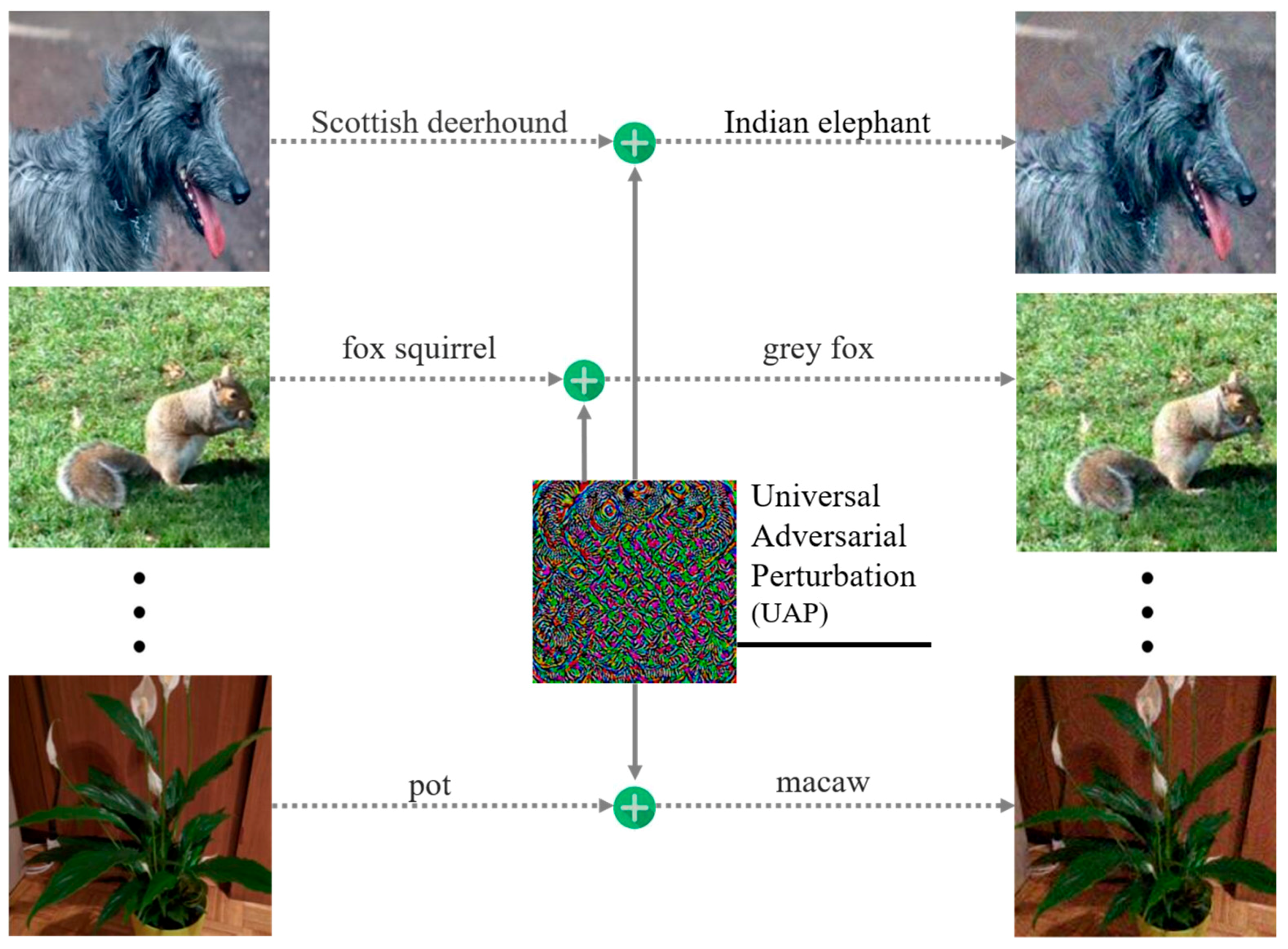
Recent work on universal adversarial perturbation (UAP) [5] shows that it is even possible to find a single adversarial perturbation that fools the target classifier on most of the examples in the dataset when added as noise to normal examples (Figure 1). UAP is a highly efficient and low-cost means for an adversary to attack a classifier. The word ‘universal’ contains a double-decked meaning on the generalization property: (1) UAPs generated for a rather small subset of a training set fool new examples with high confidence; and (2) UAPs generalize well across different DNN architectures, which is called transferability. Although the existence of UAPs implies potential regularities in adversarial perturbations, there are few effective defenses or detection methods against UAPs now.
In this paper, we propose the TwinNet framework for defending DNNs against UAPs. It separately extracts different types of features from an example for better detecting capacity. Our inspiration comes from Li et al.’s analysis [6] on adversarial examples using principal component analysis (PCA) and Molchanov et al.’s work using a double sub-network system [7] to identify hand gestures. We train an additional classifier, which performs a completely different behavior pattern from the target classifier, and then fuse their data processing results. Eventually, both of the classifiers cooperate with the detecting unit to identify the adversarial perturbation. The experimental results show that TwinNet can distinguish between normal and adversarial examples very well and is resistant to attacks with transferability.
The structure of this paper is organized as follows: Section 2 presents the related work. Section 3 describes the threat model. Section 4 demonstrates the framework architecture and the process of training shadow classifier in detail. Section 5 describes the experiment and evaluation. Conclusions and future work are presented in Section 6.
2. Related Work
2.1. Deep Neural Networks
A Deep Neural Network (DNN) consists of many nonlinear functions called neurons, which are organized in an architecture of multiple successive layers. These layers move forward progressively to build a simpler abstract representation of the high-dimensional example space, and they are connected through links weighted by a set of vectors evaluated during the training phase [8]. We call the output vector of each layer the ‘activations’.
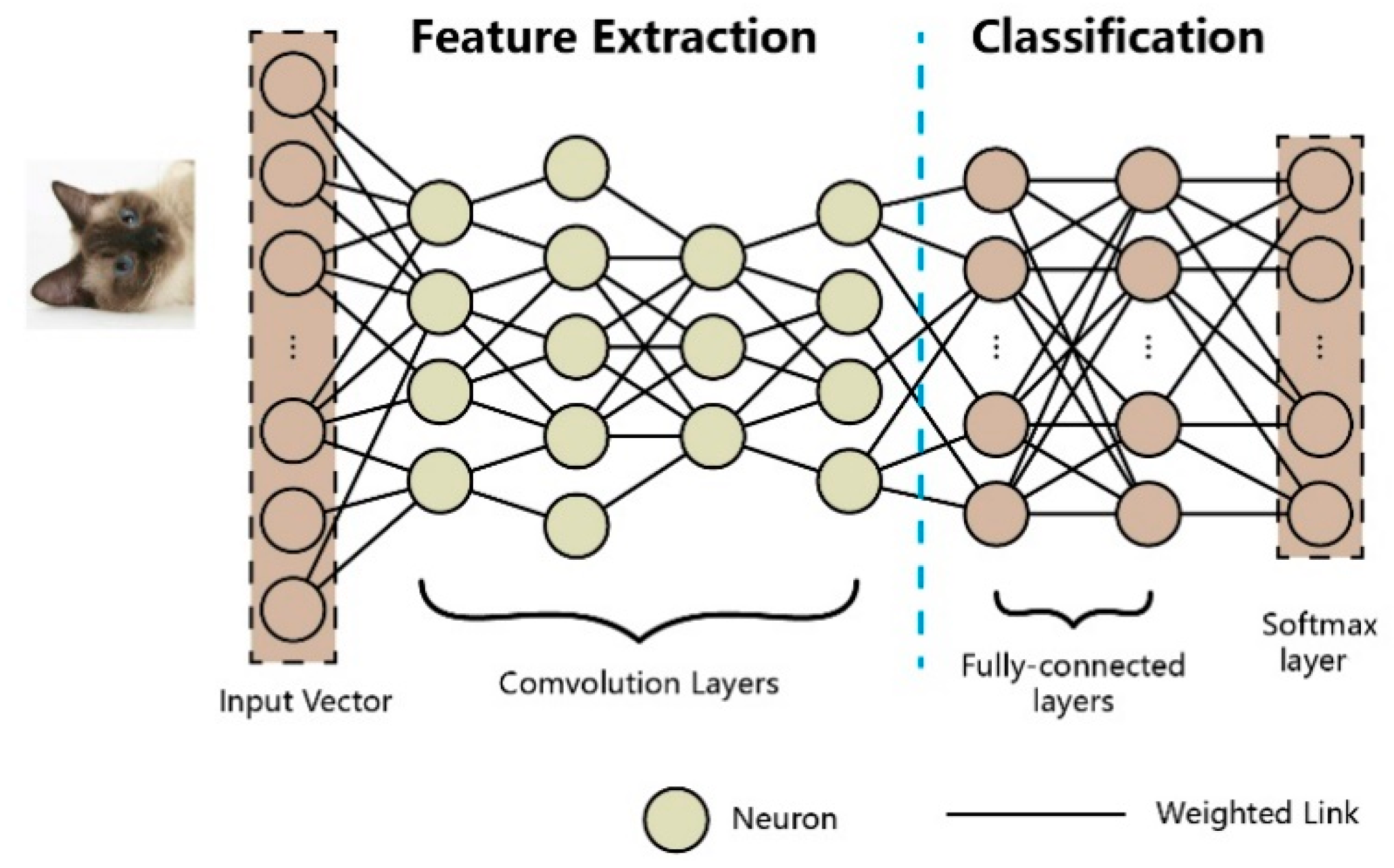
Most DNN architectures can be separated into the two function modules of feature extraction and classification (Figure 2). Feature extraction contains all convolutional layers, where each layer is a higher abstract representation of the previous one, while feature classification contains fully connected layers and a softmax layer, which actually do the classification. Layers between the input layer and the softmax layer are called hidden layers.
2.2. Existing Adversarial Attacks and Defenses
All of the existing adversarial attacks on DNNs are essentially gradient-based attacks. These attacks can be divided into standalone perturbations, transfer attacks, and universal adversarial perturbations according to the way that the adversarial perturbations are crafted.
Standalone perturbations. The crafting of standalone perturbations [2,4,9] requires referring to knowledge of the training data and the target classifier directly. In these attacks, the adversary either iteratively modifies the input features which have high impacts on the objective function, or tries to find the nearest decision boundary around the example in geometry space and traverse it. The perturbation only works for the example which it is crafted from.
Transfer attacks. Such attacks [3,10], the so-called black-box attacks, have no arbitrary access to the target classifier. A substitute, which performs the same task, will be trained locally using a synthetic dataset constructed by the adversary. As a result of transferability, adversarial perturbations crafted against the local substitute can fool the target classifier too.
Universal adversarial perturbation (UAP). It is an adversarial perturbation that is computed with few examples and removes the image-dependency of adversarial perturbations [5]. UAP exploits the inherent properties of a DNN to modify normal examples with a perturbation vector of a pretty small magnitude. It works by simply perturbating the image examples with a single pre-computed vector. While it takes more time and computing resources compared to other attacks, UAP possesses such a strong capacity of generalization that the classifier will be fooled on most new examples with the same perturbation. Furthermore, one UAP can also deceive classifiers adopting different network architectures.
There have been some efforts to protect deep neural networks against the attacks mentioned above. Compared to the defenses which aim to increase a classifier’s robustness [1,11,12] or conceal the gradient information [13,14], perturbation detection makes no modification to the target classifier and preserves classification accuracy for legitimate users to the greatest possible extent.
Some research has tried to detect adversarial perturbations using a synthetic training set [15,16] or statistics from intermediate layers [6] rather than rectifying them. This basically includes an additional classifier working as the detector to discriminate between adversarial and normal examples. The additional classifier here is generally designed for solving binary classification problems, and are auxiliary networks of the target classifier. However, the target classifier and the detector in these methods can be attacked simultaneously by fine-tuning the perturbation.
Detecting universal adversarial perturbations remains a pending issue and only a few works have taken this into consideration so far. Sengupta et al. [17] proposed a framework against UAP attacks called the MTD-NN framework. The framework assembles different networks and periodically selects the most appropriate one for the classification task. This process runs with a randomization technique; the adversary, therefore, has no idea about which is the specific target classifier and fails to attack. Unfortunately, it requires prior knowledge about the probability of attacks before making a decision. They have not provided instructions for automatic network switching when the probability of attacks is unknown. Additionally, they ignore the threat of a transfer attack.
TwinNet also employs an additional network, which is called the shadow classifier. Contrary to previous work, we do not leave all of the detecting work to the additional network. Instead, networks in TwinNet work in parallel and adopt a different metric to identify adversarial perturbations, which they can use to avoid being attacked simultaneously. Moreover, PCA is used here to evaluate the performance of the classifier rather than as a tool for data collection [18] or detection [6].
2.3. Double Sub-Network System
Molchanov et al. [7] introduced a hand gesture recognition system which utilizes three-dimensional (3D) convolutional neural networks along with depth and intensity channels. The information in these two channels is used to build normalized spatio-temporal volumes which will be fed to two separate sub-networks dedicated to processing depth and intensity features, respectively. It was proved that the double sub-network system helps in improving the accuracy of classification tasks which contain multiple types of features by dispatching different features to specialized networks and fusing the outputs later.
3. Threat Model
Popular adversarial perturbations are image-dependent, tiny vectors that make classifiers wrongly classify normal examples. Formally, we define F as a classifier that outputs the predicted label F(x) for a given example x. An adversary can generate a perturbation r specific to x to make the classifier label corresponding to the adversarial example as F(x + r), F(x + r) ≠ F(x). Additionally, r is not distinct enough to be perceived by human beings.
However, UAP is independent of image examples. It is a kind of perturbation that can fool a classifier on almost all examples sampled from a natural distribution with a single vector. Let X denote the subset containing the majority of the examples in the dataset. Then, a UAP against classifier F, referred to as v, satisfies
Most image-dependent adversaries achieve a malicious goal by imposing the least costly perturbations in the direction towards the adjacent classification region. The example that has been attacked eventually leaves the original classification region. However, a UAP generation algorithm requires a rather small subset of the training set, which proceeds by sequentially aggregating the minimal perturbations that can push successive datapoints in the subset to their respective decision boundary. These UAPs lie in a low-dimensional subspace that captures the correlations among different regions of the decision boundary, which makes it universal [5].
4. Method
TwinNet is a framework for detecting universal adversarial perturbations. This section will present the properties of adversarial perturbation, describe the architecture of the TwinNet framework, and explain how to train a shadow classifier in detail and identify adversarial perturbations.
4.1. Properties of Adversarial Perturbations
For most ML tasks, normal examples are on a manifold that is of much lower dimension than the entire example space, while adversarial ones are off this manifold [19]. Besides this, each layer in a DNN architecture can be seen as a nonlinear function on a linear transformation. The linear transformation part is responsible for most learning work, where activations are multiplied by weights and the sum with biases is added. Inspired by the work of Li et al. [6], we apply Principle Component Analysis (PCA) [20] to the activations of the first fully connected layer of a DNN, which may help to analyze the distribution of examples in low-dimensional space and explore potential difference in the way that a DNN processes both types of examples.
We perform a linear PCA on the whole collection of 5000 normal examples randomly selected from the ImageNet [21] validation set as well as 5000 corresponding universal adversarial examples. Figure 3a shows the PCA projection onto two prominent directions (the 1st and 2nd eigenvector): adversarial examples nearly belong to the same distribution as normal examples. However, it appears that adversarial examples gather more closely in the center, which indicates a significantly lower standard deviation. In Figure 3b, as we move to the tail of the PCA projection space (the 890th and 891st eigenvector), a similar phenomenon appears while both types of examples are turned to be similar to random samples under a Gaussian distribution. We also conduct the same processing on the CIFAR-10 [22] testing set (Figure 3c,d), and it shows a similar phenomenon to that described above.
According to the above observation, we can reason about the property that features of adversarial examples, compared to those of normal examples, are not obvious in those DNN classifiers trained on normal examples. An explanation for that could be that DNN classifiers impose a strong regularization effect on adversarial examples in almost all of the informative directions. The features emphasized by a classifier during the training phase tend to reflect the normality of examples, and we call them normal-related features. However, the same features in an adversarial example are suppressed. The critical features modified by an adversary, what we call adversarial-related features, are enhanced instead.
The normal-related features and adversarial-related features are partially overlapped, which explains the poor performance of adversarial training on defending DNNs against adversarial perturbations [5]. So, they can hardly be separated. Inspired by Molchanov et al.’s [7] work on processing depth and intensity features in different classifiers to improve the accuracy of hand gesture identification, we devise an additional classifier to enhance adversarial-related features. Additionally, the target classifier remains a classifier emphasizing normal-related features.
4.2. Architecture of the TwinNet Framework
A TwinNet framework comprises two sub-networks sharing the same network architecture (Figure 4), which are used to enhance normal-related features and adversarial-related features respectively: one is the target classifier , which is a popular DNN classifier, and the other is the shadow classifier , which is trained based on . These two sub-networks have exactly the same parameters for their feature extraction layers while maintaining different parameters for their classification layers independently. When it comes to normal examples, and will output normal and adversarial results, respectively. As for adversarial examples, they will both output adversarial results.
The detecting unit is responsible for fusing the results output by the sub-networks. According to the fusion result, TwinNet will determine the type of example and adopt different strategies: if example was evaluated as adversarial, it would be rejected by the system; If not, a classification label would be computed based on the output of , because , which is trained for legitimate users, possesses better classification accuracy on normal examples. The detailed mechanism of the fusion method and the evaluation criterion are presented in Section 4.4.
Formally, let denote the output vector of sub-networks in TwinNet for a given input example . Thus, is the set of class-membership probabilities for classes that equals to
where denotes the common parameters shared by two sub-networks; and and are the classification layer parameters of and , respectively. Furthermore, the detection rule is
where the label is the corresponding class of the highest element in the vector output by if the example is evaluated as normal.
4.3. Shadow Classifier
The shadow classifier runs in parallel with the target classifier . In comparison with , is dedicated to enhancing adversarial-related features. Whether it is fed a normal or an adversarial example, always produces the same result as what outputs given the corresponding adversarial example.
Hybrid training Set. In order to selectively enhance adversarial-related features in an example, is fully trained on a synthetic, specially labelled dataset called a hybrid training set, which is by definition the product mixture of two types of examples as follows
where is the classification function of the target classifier, which predicts the label for the input example ; and are the universal adversarial perturbations. In the hybrid training set , the former tuple is the normal part containing the normal examples labelled with the corresponding adversarial labels for suppressing the normal-related features. Additionally, the latter is the adversarial part containing the adversarial examples and the labels for more obvious adversarial-related features.
Furthermore, all of the examples collected in a hybrid training set are ‘bottleneck values’. We refer to the term of ‘bottleneck value’ as the activations of the layer just before the classification layers. The details of constructing a hybrid training set are described in Algorithm 1.
| Algorithm 1 Constructing Hybrid Training Set |
| Input: ←normal example set, ←classification function of target classifier, ←universal adversarial perturbation |
| Output: ←hybrid training set |
| 1: Initialize ← |
| 2: for in : |
| 3: if |
| 4: ←classification label |
| 5: ←bottleneck activations of |
| 6: ←bottleneck activations of |
| 7: ← |
| 8: ← |
| 9: return |
Training. Considering time and computing resources, is retrained from on a hybrid training set using the transfer learning technique [23]. Transfer learning is a technique which shortcuts a lot of work of parameter training by taking a fully trained model for a set of categories, and retraining from the existing weights for new classes. Eventually, only the parameters of the classification layers are learned from scratch, leaving those of the feature extraction layers unchanged. We therefore collect bottleneck values in a hybrid training set rather than in original image examples.
4.4. Identifying Adversarial Perturbations
In most multiple network detection systems, a detector’s property of passive access to information makes it possible that the target classifier and the detector will be attacked simultaneously. An adversary can fine-tune the perturbation referring to the detector’s objective to make it undetectable again. In TwinNet, however, there is no data exchange between two oppositely working sub-networks. Additionally, the final decision will be made by the independent detecting unit.
We use cosine as the detection criterion in the detecting unit. Thus, the difference between the outputs of the target classifier and the shadow classifier is
where denotes the ith component of the output vector of classifier for a given example . The range of the cosine value is . The larger the cosine value, the smaller the angle between output vectors, and vice versa. The criteria for evaluating an example as normal or adversarial by cosine values is
where T is the threshold for detecting whose value is empirically chosen.
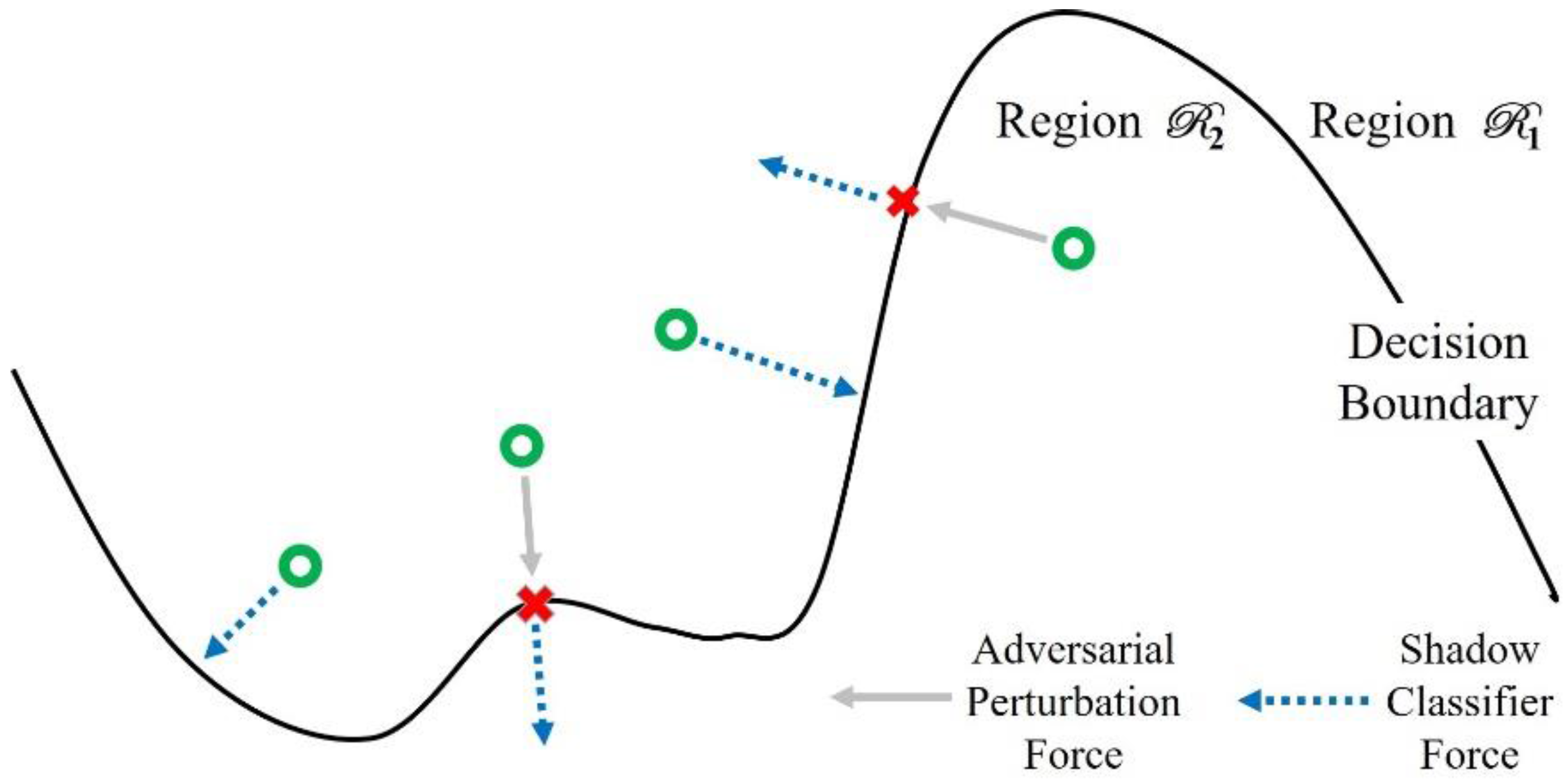
As a result of the construction of a hybrid training set, the shadow classifier has a bias towards adversarial-related features, which redraws decision boundaries different from that of the target classifier. From the geometric point of view, adversarial examples go deeper smoothly into the the adjacent classification region while normal examples leap over a decision boundary directly into the shadow classifier (Figure 5).
Thus, the rationale behind using an angle as the key metric to measure the difference between output vectors is that, in terms of using a target classifier and a shadow classifier, the direction of the output vector changes smoothly in adversarial examples. By contrast, it changes dramatically in normal examples. Therefore, the angle of the output vector between two sub-networks in adversarial examples should be smaller than that in normal examples, no matter how adversarial perturbation is fine-tuned. It is going to be harder for an adversary to attack all classifiers in TwinNet at the same time.
5. Experiment
5.1. Setting
Our framework was implemented based on the Tensorflow machine learning library. The shadow classifier was retrained from the classifier to be tested using the transfer learning technique [23] and the stochastic gradient descent optimization algorithm [24]. Table 1 shows the training parameters of the shadow classifier.
Our framework was tested on six different classifier architectures (Table 2) which have been sufficiently trained and validated on the ILSVRC-2012 dataset [21]. We used six distinct pre-computed UAPs [25] as the attacks taken by an adversary. These UAPs were generated based on the architectures mentioned above, respectively, with their norms restricted within a bound of . We took 5000 examples randomly selected from the ILSVRC-2012 test set, along with their corresponding universal adversarial examples, as the validation set. The validation set contained examples from 1000 categories and each category had 10 examples. Each example was a RGB image.
In the rest of this section, we show the performance of the shadow classifier. Then, we evaluate the robustness of TwinNet against UAPs and a transfer attack. Finally, scatter plots of the detection result are provided to demonstrate that TwinNet works well in differentiating normal and universal adversarial examples. The indicators we use to measure the detecting performance are the fooling rate (the proportion of adversarially perturbed examples being wrongly predicted by the classifier), the detecting hit rate (the proportion of adversarial examples being detected successfully), and the false alarm rate (the proportion of normal examples being wrongly evaluated as adversarial).
5.2. Experiment Results and Analysis
Figure 6a shows the PCA projection of the activations output by the shadow classifier onto the 1st and 2nd eigenvectors. The adversarial part, in comparison to how the target classifier performs (Figure 6c), appears more dispersed and even covers the normal part, which indicates a higher standard deviation. It demonstrates that the shadow classifier can effectively enhance adversarial-related features. When we move to the tail of the projection space (Figure 6b), the distribution of the examples is similar to that of the target classifier (Figure 6d).
Table 2 shows six different network architectures that we test on and compares the fooling rate of UAPs before and after applying our framework. Each classifier is tested by the UAP, which is generated with knowledge of the classifier itself. For example, the classifier GoogLeNet is tested by the UAP generated with knowledge of GoogLeNet.
We can see that TwinNet can significantly improve the robustness of all of the test classifiers. Additionally, in the best case (CaffeNet), TwinNet is able to reduce the damage brought by the UAP from 93.3% to 29.79%. This is the best result up to now.
In Table 3, we show the detection performance of TwinNet in more detail (T = 0.45).
TwinNet is good not only at detecting adversarial perturbations, but it is also good at maintaining a high accuracy on normal examples. Moreover, the robustness of TwinNet across different architectures remains stable consistently such that it can get an average detecting hit rate of up to 72.67%, and even the worst case of VGG-F can reach 66.55%, which is much better than that of existing works.
In Table 4, we evaluate the performance of TwinNet defending GoogLeNet against a transfer attack (T = 0.45). The fields of the first column are the network architectures used to craft UAPs by the adversary.
The UAPs used here are generated with knowledge of the remaining five classifiers. We find that TwinNet, with the detecting threshold of 0.45, is practically immune to the transfer attack. It always maintains a high detecting hit rate and a low false alarm rate, reaching 70.27% and 6.45%, respectively, on average. We also note that the network of VGG-F is relatively hard to protect.
In Figure 7, we compare the accuracy of classifiers that have applied TwinNet and MTD-NN [17] when the proportion of adversarial examples in the validation set varies. It shows that as the proportion increases, the polylines of TwinNet lie above those of MTD-NN. Thus, TwinNet outperforms MTD-NN on the same dataset.
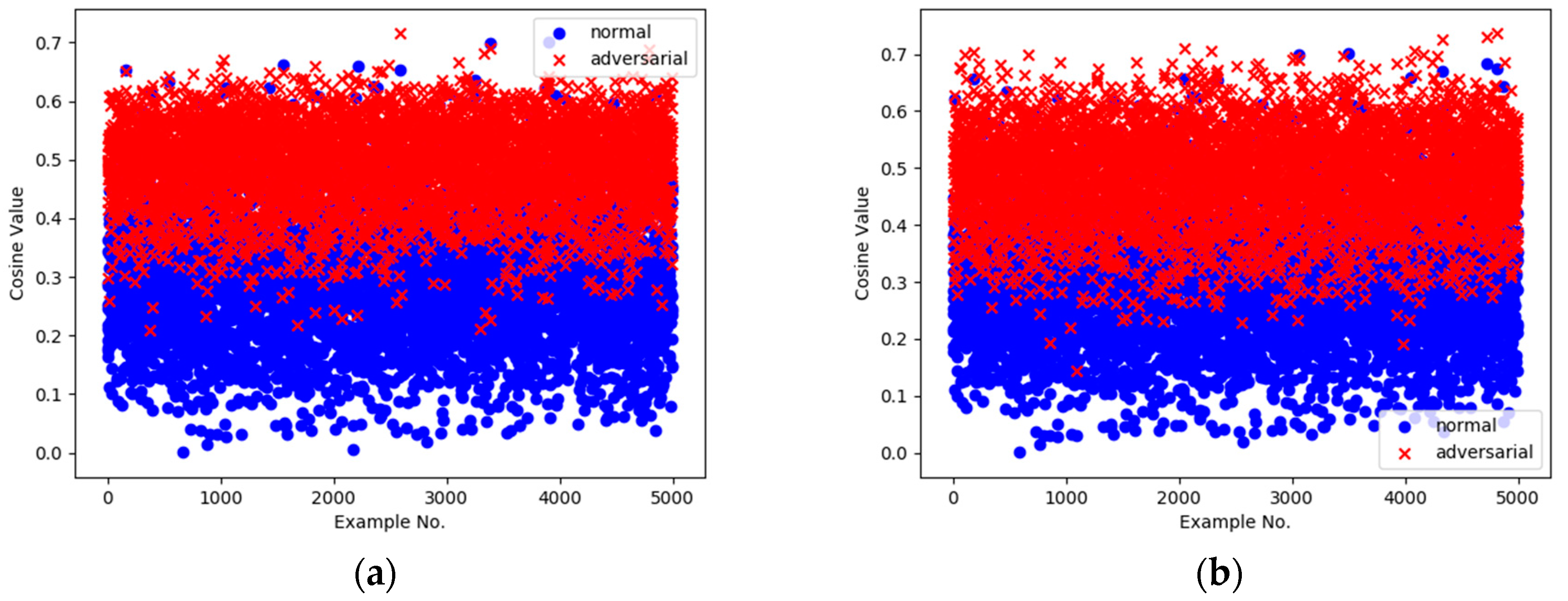
Illustrated by the case of GoogLeNet, we plot the distribution of the detecting results, that is cosine values, of all of the examples in the validation set in Figure 8a. It shows that there is obviously a hierarchical differentiation between the normal and adversarial parts, which proves that a connection exists between the underlying mechanism of TwinNet and the direction of the examples. Figure 8b demonstrates that the same detecting threshold of 0.45 generalizes well across UAPs generated based on different architectures.
6. Conclusions
As the DNN technique has become more mature, a security problem along with its prevalence has been noticed. In particular, a universal adversarial perturbation (UAP) can fool the classifier on almost all examples with a single perturbation vector, and it is short of effective defenses. We propose TwinNet, a framework for DNN systems to detect UAP attacks. TwinNet processes examples with two sub-networks: one is a target classifier which focuses on normal-related features and the other is a shadow classifier dedicated to making adversarial-related features more enhanced. These two networks and a detecting unit work jointly to identify universal adversarial perturbations. The framework can be applied to most DNN architectures, and can avoid the situation that all networks are fooled simultaneously to the greatest possible extent. Experiments show that TwinNet can effectively distinguish between normal examples and adversarial examples. It can achieve a detecting accuracy which significantly outperforms state-of-the-art work along with a low false alarm rate. In future work, on the one hand, more network architectures will be tested for a more thorough assessment of TwinNet. On the other hand, we will explore the possibility of using UAP-trained TwinNet to detect other popular adversarial perturbations.
Acknowledgments
This work was supported by the Innovation Program of the Shanghai Municipal Education Commission (Grant No. 13YZ013), the State Scholarship Fund of the China Scholarship Council (Grant NO.201606895018), and the Natural Science Foundation of Shanghai Municipality (Grant No.17ZR1409800).
Author Contributions
Yibin Ruan is the main author of this article. All the authors have contributed to this manuscript. All authors have read and approved the final manuscript.
Conflicts of Interest
The authors declare no conflict of interest.
References
- Szegedy, C.; Zaremba, W.; Sutskever, I.; Bruna, J.; Erhan, D.; Goodfellow, I.; Fergus, R. Intriguing properties of neural networks. arXiv, 2013; arXiv:1312.6199. [Google Scholar]
- Moosavi-Dezfooli, S.M.; Fawzi, A.; Frossard, P. Deepfool: A simple and accurate method to fool deep neural networks. In Proceedings of the 2016 IEEE Conference on Computer Vision and Pattern Recognition (CVPR), Seattle, WA, USA, 27–30 June 2016; pp. 2574–2582. [Google Scholar]
- Papernot, N.; Mcdaniel, P.; Goodfellow, I.; Jha, S.; Celik, Z.B.; Swami, A. Practical black-box attacks against deep learning systems using adversarial examples. arXiv, 2016; arXiv:1602.02697. [Google Scholar]
- Kurakin, A.; Goodfellow, I.; Bengio, S. Adversarial examples in the physical world. arXiv, 2016; arXiv:1607.02533. [Google Scholar]
- Moosavidezfooli, S.M.; Fawzi, A.; Fawzi, O.; Frossard, P. Universal adversarial perturbations. arXiv, 2016; arXiv:1610.08401. [Google Scholar]
- Li, X.; Li, F. Adversarial examples detection in deep networks with convolutional filter statistics. arXiv, 2016; arXiv:1612.07767. [Google Scholar]
- Molchanov, P.; Gupta, S.; Kim, K.; Kautz, J. Hand gesture recognition with 3d convolutional neural networks. In Proceedings of the IEEE Conference on Computer Vision and Pattern Recognition Workshops, Boston, MA, USA, 8–10 June 2015; pp. 1–7. [Google Scholar]
- Goodfellow, I.; Bengio, Y.; Courville, A. Deep Learning; MIT Press: Cambridge, MA, USA, 2016. [Google Scholar]
- Goodfellow, I.J.; Shlens, J.; Szegedy, C. Explaining and harnessing adversarial examples. arXiv, 2014; arXiv:1412.6572. [Google Scholar]
- Narodytska, N.; Kasiviswanathan, S.P. Simple black-box adversarial perturbations for deep networks. arXiv, 2016; arXiv:1612.06299. [Google Scholar]
- Kurakin, A.; Goodfellow, I.; Bengio, S. Adversarial machine learning at scale. arXiv, 2016; arXiv:1611.01236. [Google Scholar]
- Zheng, S.; Song, Y.; Leung, T.; Goodfellow, I. Improving the robustness of deep neural networks via stability training. In Proceedings of the IEEE Conference on Computer Vision and Pattern Recognition, Seattle, WA, USA, 27–30 June 2016; pp. 4480–4488. [Google Scholar]
- Papernot, N.; Mcdaniel, P.; Wu, X.; Jha, S.; Swami, A. Distillation as a defense to adversarial perturbations against deep neural networks. In Proceedings of the 2016 IEEE Symposium on Security and Privacy, San Jose, CA, USA, 23–25 May 2016. [Google Scholar]
- Lu, J.; Issaranon, T.; Forsyth, D. Safetynet: Detecting and rejecting adversarial examples robustly. arXiv, 2017; arXiv:1704.00103. [Google Scholar]
- Metzen, J.H.; Genewein, T.; Fischer, V.; Bischoff, B. On detecting adversarial perturbations. arXiv, 2017; arXiv:1702.04267. [Google Scholar]
- Meng, D.; Chen, H. Magnet: A two-pronged defense against adversarial examples. In Proceedings of the 2017 ACM SIGSAC Conference on Computer and Communications Security, Dallas, TX, USA, 30 October–3 November 2017. [Google Scholar]
- Sengupta, S.; Chakraborti, T.; Kambhampati, S. Securing deep neural nets against adversarial attacks with moving target defense. arXiv, 2017; arXiv:1705.07213. [Google Scholar]
- Bhagoji, A.N.; Cullina, D.; Mittal, P. Dimensionality reduction as a defense against evasion attacks on machine learning classifiers. arXiv, 2017; arXiv:1704.02654. [Google Scholar]
- Tanay, T.; Griffin, L. A boundary tilting persepective on the phenomenon of adversarial examples. arXiv, 2016; arXiv:1608.07690. [Google Scholar]
- Jolliffe, I.T. Principal Component Analysis; Springer: New York, NY, USA, 2005; pp. 41–64. [Google Scholar]
- Russakovsky, O.; Deng, J.; Su, H.; Krause, J.; Satheesh, S.; Ma, S.; Huang, Z.; Karpathy, A.; Khosla, A.; Bernstein, M. Imagenet large scale visual recognition challenge. Int. J. Comput. Vis. 2015, 115, 211–252. [Google Scholar] [CrossRef]
- Krizhevsky, A. Learning Multiple Layers of Features from Tiny Images; Tech Report; University of Toronto: Toronto, ON, Canada, 2009. [Google Scholar]
- Donahue, J.; Jia, Y.; Vinyals, O.; Hoffman, J.; Zhang, N.; Tzeng, E.; Darrell, T. Decaf: A deep convolutional activation feature for generic visual recognition. In Proceedings of the International Conference on Machine Learning, Beijing, China, 21–26 June 2014. [Google Scholar]
- Hardt, M.; Recht, B.; Singer, Y. Train faster, generalize better: Stability of stochastic gradient descent. arXiv, 2015; arXiv:1509.01240. [Google Scholar]
- Moosavidezfooli, S.M.; Fawzi, A.; Fawzi, O.; Frossard, P. Precomputed Universal Perturbations for Different Classification Models. Available online: https://github.com/LTS4/universal/tree/master/precomputed (accessed on 11 March 2017).
- Szegedy, C.; Liu, W.; Jia, Y.; Sermanet, P.; Reed, S.; Anguelov, D.; Erhan, D.; Vanhoucke, V.; Rabinovich, A. Going deeper with convolutions. arXiv, 2014; arXiv:1409.48427. [Google Scholar]
- Jia, Y.; Shelhamer, E.; Donahue, J.; Karayev, S.; Long, J.; Girshick, R.; Guadarrama, S.; Darrell, T. Caffe: Convolutional architecture for fast feature embedding. In Proceedings of the 22nd ACM International Conference on Multimedia, San Francisco, CA, USA, 27 October–1 November 2013; pp. 675–678. [Google Scholar]
- Chatfield, K.; Simonyan, K.; Vedaldi, A.; Zisserman, A. Return of the devil in the details: Delving deep into convolutional nets. arXiv, 2014; arXiv:1405.3531. [Google Scholar]
- Simonyan, K.; Zisserman, A. Very deep convolutional networks for large-scale image recognition. arXiv, 2014; arXiv:1409.1556. [Google Scholar]
- He, K.; Zhang, X.; Ren, S.; Sun, J. Deep residual learning for image recognition. In Proceedings of the Computer Vision and Pattern Recognition, Seattle, WA, USA, 27–30 June 2016; pp. 770–778. [Google Scholar]
Figure 1.
Universal adversarial perturbation.

Figure 2.
The architecture of a deep neural network.

Figure 3.
Scatter plots of principal component analysis (PCA) projection of activations at the first fully connected layer onto specific eigenvectors in the target classifier. Blue area indicates normal examples and red area indicates adversarial ones. Illustrated by the case of the ImageNet validation set: (a) projection onto the 1st and 2nd eigenvectors; (b) projection onto the 890th and 891st eigenvectors. Illustrated by the case of the MNIST testing set: (c,d) are projections onto the same eigenvectors as (a,b), respectively.
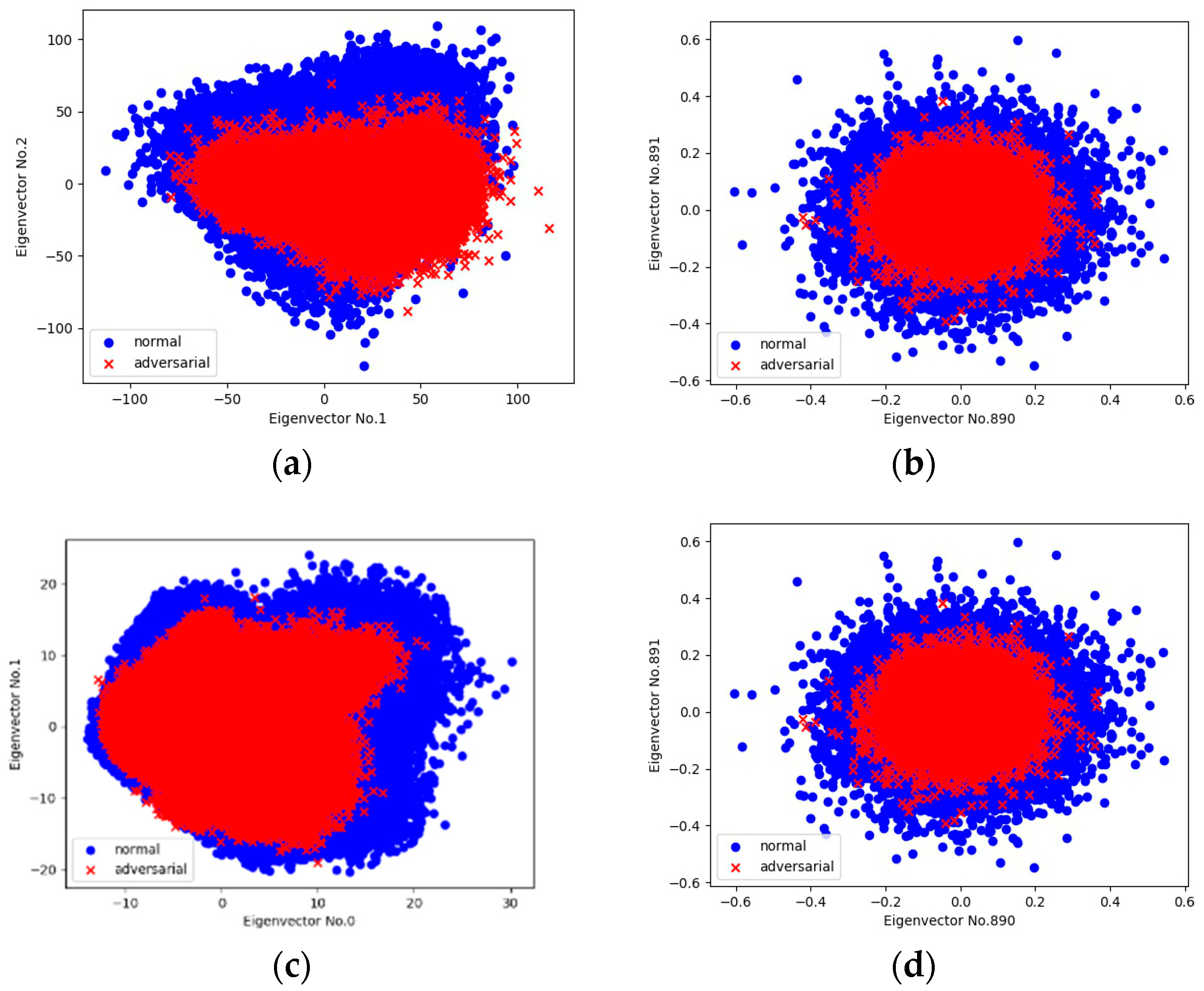
Figure 4.
Architecture of the TwinNet framework.

Figure 5.
Schematic representation of how shadow classifier works in a two-dimensional (2D) example space. We depict normal and adversarial examples by green dots and red crosses, respectively.
Figure 5.
Schematic representation of how shadow classifier works in a two-dimensional (2D) example space. We depict normal and adversarial examples by green dots and red crosses, respectively.

Figure 6.
Scatter plots of PCA projection of activations at the first fully connected layer onto specific eigenvectors. Blue area indicates normal examples and red area indicates adversarial ones: in the shadow classifier, (a) projection onto the 1st and 2nd eigenvectors; (b) projection onto the 890th and 891st eigenvectors; in the target classifier, (c) projection onto the 1st and 2nd eigenvectors; (d) projection onto the 890th and 891st eigenvectors.

Figure 7.
Accuracy of the deep neural network (DNN) when the proportion of adversarial example in the validation set varies.
Figure 7.
Accuracy of the deep neural network (DNN) when the proportion of adversarial example in the validation set varies.
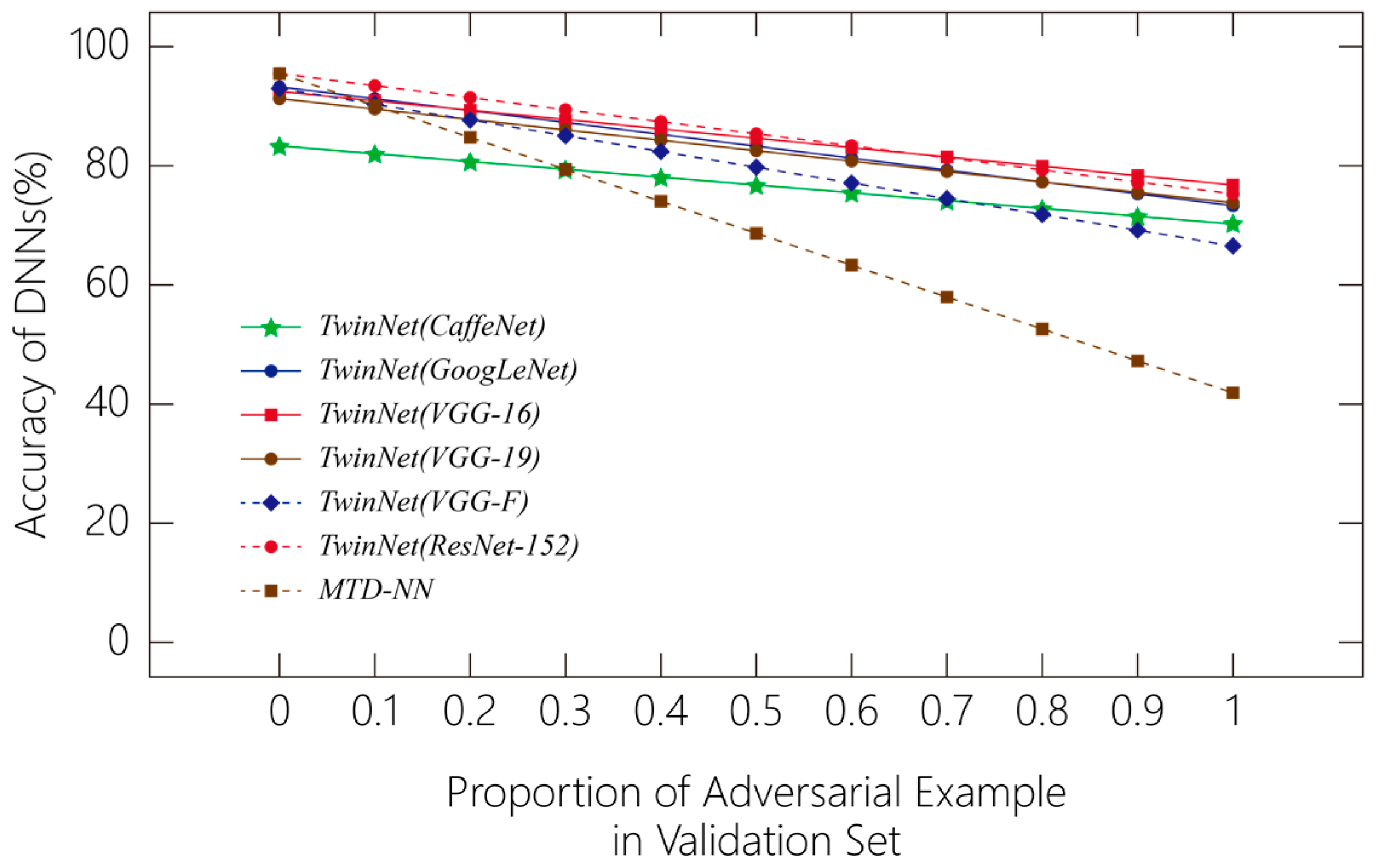
Figure 8.
Scatter plot of fusion result of examples in the validation set. The x axis is the example number, and the y axis is the corresponding cosine value. (a) Adversary uses the same UAP as the one applied during the training phase; (b) Adversary uses the UAP generated on a different architecture.

Table 1.
Training parameters of the shadow classifier.
| Parameters | Values |
|---|---|
| Training Method | transfer learning |
| Optimization Method | stochastic gradient descent (SGD) |
| Learning Rate | 0.001 |
| Dropout | - |
| Batch Size | 100 |
| Steps | 28,000 |
Table 2.
Classification accuracy of six network architectures on normal examples and the fooling rate that the UAP reached before and after applying the TwinNet framework.
Table 2.
Classification accuracy of six network architectures on normal examples and the fooling rate that the UAP reached before and after applying the TwinNet framework.
| Network Architecture | Classification Accuracy/(%) | Fooling Rate/(%) | Fooling Rate (applying TwinNet)/(%) |
|---|---|---|---|
| GoogLeNet [26] | 93.3 | 78.9 | 26.68 |
| CaffeNet [27] | 83.6 | 93.3 | 29.79 |
| VGG-F [28] | 92.9 | 93.7 | 33.45 |
| VGG-16 [29] | 92.5 | 78.3 | 23.17 |
| VGG-19 [29] | 92.5 | 77.8 | 26.19 |
| ResNet-152 [30] | 95.5 | 84 | 24.7 |
Table 3.
Detection performance of the TwinNet framework for six network architectures on 10-class ImageNet.
Table 3.
Detection performance of the TwinNet framework for six network architectures on 10-class ImageNet.
| Network Architecture | Detecting Hit Rate/% | False Alarm Rate/% |
|---|---|---|
| GoogLeNet | 73.32 | 6.06 |
| CaffeNet | 70.21 | 6.23 |
| VGG-F | 66.55 | 6.5 |
| VGG-16 | 76.83 | 6.01 |
| VGG-19 | 73.81 | 6.06 |
| ResNet-152 | 75.3 | 6.08 |
Table 4.
Robustness of the TwinNet framework for defending GoogLeNet against a transfer attack on 10-class ImageNet.
Table 4.
Robustness of the TwinNet framework for defending GoogLeNet against a transfer attack on 10-class ImageNet.
| Network Architecture of Adversary | Detecting Hit Rate/(%) | False Alarm Rate/(%) |
|---|---|---|
| CaffeNet | 67.84 | 6.7 |
| VGG-F | 58.76 | 6.3 |
| VGG-16 | 76.54 | 6.76 |
| VGG-19 | 73.22 | 6.26 |
| ResNet-152 | 75 | 6.26 |
© 2018 by the authors. Licensee MDPI, Basel, Switzerland. This article is an open access article distributed under the terms and conditions of the Creative Commons Attribution (CC BY) license (http://creativecommons.org/licenses/by/4.0/).
Share and Cite
MDPI and ACS Style
Ruan, Y.; Dai, J. TwinNet: A Double Sub-Network Framework for Detecting Universal Adversarial Perturbations. Future Internet 2018, 10, 26. https://doi.org/10.3390/fi10030026
AMA Style
Ruan Y, Dai J. TwinNet: A Double Sub-Network Framework for Detecting Universal Adversarial Perturbations. Future Internet. 2018; 10(3):26. https://doi.org/10.3390/fi10030026
Chicago/Turabian StyleRuan, Yibin, and Jiazhu Dai. 2018. "TwinNet: A Double Sub-Network Framework for Detecting Universal Adversarial Perturbations" Future Internet 10, no. 3: 26. https://doi.org/10.3390/fi10030026
Note that from the first issue of 2016, this journal uses article numbers instead of page numbers. See further details here.