Optimal Design of Demand-Responsive Feeder Transit Services with Passengers’ Multiple Time Windows and Satisfaction

1
School of Transportation, Nantong University, Nantong 226019, China
2
Nantong Research Institute for Advanced Communication Technologies, Nantong 226019, China
3
College of Civil Engineering, Hebei University of Technology, Tianjin 300401, China
*
Author to whom correspondence should be addressed.
Future Internet 2018, 10(3), 30; https://doi.org/10.3390/fi10030030
Submission received: 19 January 2018
/
Revised: 21 February 2018
/
Accepted: 8 March 2018
/
Published: 12 March 2018
(This article belongs to the Special Issue New Perspectives in Intelligent Transportation Systems and Mobile Communications towards a Smart Cities Context)
Abstract
:This paper presents a mixed-integer linear programming model for demand-responsive feeder transit services to assign vehicles located at different depots to pick up passengers at the demand points and transport them to the rail station. The proposed model features passengers’ one or several preferred time windows for boarding vehicles at the demand point and their expected ride time. Moreover, passenger satisfaction that was related only to expected ride time is fully accounted for in the model. The objective is to simultaneously minimize the operation costs of total mileage and maximize passenger satisfaction. As the problem is an extension of the nondeterministic polynomial problem with integration of the vehicle route problem, this study further develops an improved bat algorithm to yield meta-optimal solutions for the model in a reasonable amount of time. When this was applied to a case study in Nanjing City, China, the mileage and satisfaction of the proposed model were reduced by 1.4 km and increased by 7.1%, respectively, compared with the traditional model. Sensitivity analyses were also performed to investigate the impact of the number of designed bus routes and weights of objective functions on the model performance. Finally, a comparison of Cplex, standard bat algorithm, and group search optimizer is analyzed to verify the validity of the proposed algorithm.
1. Introduction
The first/last mile access to major fixed-route transit networks and connectivity of residential areas is one of the main challenges faced by public transit. A feasible solution to the problem is the planning, design, and implementation of efficient feeder transit services [1,2]. Traditionally, transit services have been divided into two broad categories: the fixed route (FRT) and the demand responsive (DRT). FRTs do not match the desires of individual riders (the locations of pickup and/or drop off points) and have a predetermined schedule, while DRTs provide the desired flexibility with a door-to-door type of service [3,4]. Therefore, DRTs provide increased flexibility, lower operation costs, and a higher service level compared with FRTs, especially within low-density residential areas.
DRTs are an extension of the vehicle routing problem (VRP) and the pickup and delivery problem (PDP) with time windows [3]. This aims to assign routes in order to visit demand points and transport passengers to the rail station, where passengers can acquire travel information through a phone app. Obviously, passengers’ time windows and expected ride time affect the building process of the route. The existing DRTs assume that passengers travel only in a single period of time and neglect that passengers sometimes provide multiple time windows, with the vehicle required to arrive at the designated place within one of the specified periods to pick them up. Similar to VRPs with multiple time windows [5,6], DRTs with multiple time windows can save a greater amount of mileage compared with the single time window problem. Furthermore, it is very important for passengers to set a maximum and minimum expected ride time to meet personalized travel needs, which will encourage the drivers to take the shortest route distance in order to reduce the time in the vehicle for other passengers. However, DRTs with expected ride time have also not been examined previously.
Another major motivation for this study was to address DRTs in terms of passenger satisfaction, which involves many factors, such as bus fares, congestion, environment, etc. Some studies have studied VRPs with consideration of customer satisfaction, although this has been considered less in the DRTs [7,8]. Without loss of generality, it is only relevant in terms of expected ride time in feeder transit operation (i.e., the satisfaction is in the range of 0–1) when the ride time is between the minimum and maximum expected values. Obviously, greater passenger satisfaction and demand for more vehicles to provide direct services will increase the total mileage and operating expenses. Therefore, it is necessary to reveal the optimal relationship between passenger satisfaction and the total mileage in order to balance this with service quality and operating costs.
The main objective of this research is to develop an optimization model for DRTs with passengers’ multiple time windows and satisfaction in order to improve service quality and operating costs. The paper will focus on the following critical research tasks: (1) coordination of the passenger boarding time window guidance and feeder transit routing process to balance this with the total mileage and passenger satisfaction; and (2) development of a heuristic solution algorithm to efficiently yield the acceptable solution to the proposed mode. Finally, a numeric case study is used to illustrate the proposed methodology and apply the proposed model during the process of producing the optimal design fora DRT in the real world.
The remainder of the paper is organized as follows. Section 2 reviews the related literature onDRTs. Section 3 analyses the framework of the proposed methodology and presents the formulation of the DRT model. Section 4 presents an improved bat heuristic algorithm for resolving the model. Section 5 displays a case study to illustrate the proposed model and algorithm. Some concluding remarks and possible future work are given in Section 6.
2. Literature
DRTs are door-to-door transportation services that provide dial-a-ride pickup/delivery services [9,10,11]. They have often been described as an extension of two fundamental vehicle routing and scheduling problems [12,13], in which the vehicle routing problem (VRP) assigns some vehicles to visit a set of geographically dispersed locations, while the pickup and delivery problem (PDP) moves the number of goods from certain pickup locations to certain delivery locations. However, there are also distinct differences between the VRPs and PDPs discussed so far and DRTs. VRPs and PDPs focus on the transportation of goods, while DRTs are concerned with the transportation of people. Thus, DRTs address more additional issues and are more complex than VRPs and PDPs. Most reviews with DRTs are related to service and passenger convenience [11,14]. Since FRTs are not efficient due to low population density, DRTs perform better in these scheduling areas, especially those with a weak transportation infrastructure [15].
In general, passengers are picked up and delivered in special time windows, resulting in the VRP with time windows (VRPTW) and PDP with time windows (PDPTW)problems [16]. Ina recent review of VRPTWs and PDPTWs, another variant was found when the vehicle can immediately undertake another route after returning to the depot, which is referred to as the vehicle routing problem with multiple use of vehicles [8,17,18]. Although DRTs with multiple use of vehicles are more realistic, the main challenge in addressing multi-vehicle compared with single-vehicle DRTs involves the inability of direct applications of the solution techniques for the single use of vehicles case to search the solution space efficiently for multi-vehicle problems. Another variant arises when vehicles can return to any of these depots after picking up passengers when there are multiple depots [19,20,21]. DRTs with multiple depots are more complex than traditional ones since vehicles from different depots have different travel costs related to the distance from each depot, thus affecting the routing of all vehicles. Therefore, it is very important to choose optimal depots for each vehicle to reduce the operation costs in the problem. Other relevant studies on DRTs address the coordination between design of the passenger rail service, station spacing, the design of bus routes, and headways using integrated, robust, and bi-level programming optimization [22,23,24,25]. The above varieties of DRTs are addressed from various objectives, including minimizing the operating costs of the fleet [3,11,26], the shortest length or travel time of the route [27,28], the minimal fleet size required for shuttle service [1,22], ride time, and waiting time of passengers [4,15]. Fortunately, these objectives normally do not affect the properties of DRTs and, thus, similar models and algorithms can be adopted to solve the problem with different objectives.
As the problem belongs to NP-hard problems, heuristics are most frequently used to handle a large number of vehicle routing and scheduling variants for DRTs [29,30,31]. Some scholars have tried to develop route-building heuristics by first generating a set of feasible routes, before searching fine-tuned initial solutions [3,4,28,32]. Furthermore, these developed route-building-based heuristics, which are the three most widely used metaheuristics, are often adopted to contend with VRPTW, including evolutionary algorithm [26], genetic algorithms [27,32,33,34,35] and table search [36,37,38,39].
Although most of the aforementioned studies have successfully handled a variety of DRTs, the following critical issues deserve further investigation:
- (1)
- Traditional DRTs only consider passengers’ single time windows and few of them take multiple time windows into account. This implies a lack of integrated operation to guide passenger boarding in the specified time periods from several preferred time windows and routing of transit from selected demand points to destinations.
- (2)
- Only a few studies have considered the impact of the expected ride time of passengers, which is related to passenger satisfaction, on the vehicle routing. This implies a lack of an integrated operation that balances passenger satisfaction and operation costs.
- (3)
- DRTs are NP-hard problems as they are extensions of the classic VRPs and an efficient algorithm needs to be designed to solve this problem.
3. Methodology
3.1. Research Framework
In this paper, a DRT is proposed that provides services to conveniently transport passengers from demand points to the rail station [1,40,41]. Using a cellphone app and an open geo-information system(GIS)tool, we can obtain the traveling information of some passengers and the traffic network in the study area. Each passenger has one or several preferred boarding time windows as well as minimum and maximum expected ride times. During the process of designing the route, each vehicle starts at the dispatch center, visits the demand points to pick up passengers in the specified time periods, and arrives at the rail transit station. This is designed to meet realistic constraints, such as time windows and expected ride time, etc. To reveal the optimal relationship between passenger satisfaction and total mileage to maximize the efficiency in the feeder bus route design, a mixed-integer programming model was formulated to design routes from selected demand points to the rail station, which includes the demand points of passengers in the specified time period from several preferred time windows. These key components are illustrated by a research framework graph, shown in Figure 1.
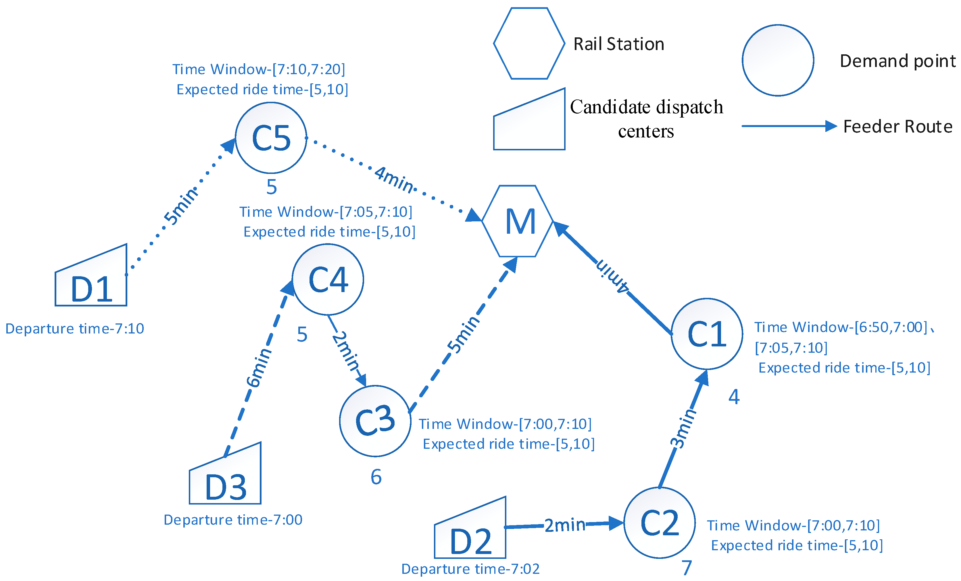
Figure 2 also provides another explanation of the principle and scope of the proposed model. Figure 2 includes one rail station (M), three dispatch centers (D1–D3), and five demand points (C1–C5) in the DRT. The numbers below each demand point (Ci, where i = 1, 2,…, 5) denotes the number of passengers in the location. Two numbers in brackets to the left of each demand point (Ci, where i = 1, 2,…, 5) denote the minimum and maximum values of preferred boarding time windows and expected ride time. For instance, the value below demand point C1 of Figure 2 is 4, which means that four people will board the bus at this location. They have two preferred boarding time windows of [6:50, 7:00] and [7:05, 7:10], while their minimum and maximum expected ride times are 5 min and 10 min. In this example, the optimization process yields three routes as follows. Route 1 is illustrated by a solid line [D1(7:10)–C5(7:15)–M(7:19)], Route 2 by a dashed line [D3(7:00)–C4(7:06)–C3(7:08)–M(7:13)], and Route 3 by a dotted line [D2(7:02)–C2(7:04)–C1(7:07)–M(7:11)]. For example, Vehicle 3 departs from D2 at 7:02, arrives at demand points C2 and C1 at the times of 7:04 and 7:07 to pick up seven and four people, respectively, before finally returning back to M at 7:11. Thus, the ride times of the two customers are 7 min and 4 min. We also define the passenger satisfaction related to demand points as the amount of ride time minus the minimum ride time divided by the amount of the maximum ride time minus the minimum ride time. In this case, passengers at C2 and C1 would get on the bus in the time periods of [7:00, 7:10] and [7:05, 7:10], respectively, with their passenger satisfactions being (10 − 7)/(10 − 5) = 0.6 and 1. In this case, the loading schemes at each stop of Route 1 can be described as {C5(5)}, while this is described for Routes 2 and 3 as {C4(5), C3(11)} and {C2(7), C1(11)}. The satisfaction at each stop of Route 1 can be described as {C5(1)}, while this is {C4(0.6), C3(1)} and {C2(0.6), C1(1)} for Routes 2 and 3. It is important to note that Route 3 may be described as [D2–C1–C2–M] with more mileage and longer ride times, if passengers at the C1 point can only be picked up in the time period of [6:50, 7:00].
Our objective is to find a subgraph that simultaneously maximizes passenger satisfaction and minimizes the total mileage cost of designed feeder routes. To ensure that the proposed DRT model fits well with the real-world situations, this study considers the following assumptions:
- (1)
- Passengers at the demand point are allowed to travel in one or several preferred boarding time windows. It is possible to investigate the number of passengers at each demand point around the rail station and ignore the passenger flow between them.
- (2)
- The distance and travel time between demand points, dispatch centers, and rail stations are obtained using Baidu GIS.
- (3)
- Each demand point can only be covered once by one vehicle.
- (4)
- The passenger’s satisfaction is only related with her/his ride time. The reduction in passenger satisfaction can be estimated.
3.2. Model Formulation
3.2.1. Notation
To facilitate the model presentation, all definitions and notation used hereafter are summarized in Table 1.
3.2.2. Formulation
The proposed problem can be formulated as the following mixed-integer program (MIP), which requires minimization of
subject to
where is a function used to calculate the satisfaction of passengers at the demand point based on his/her ride time , with the arrival time for the vehicle visiting the demand point i satisfying one of its multiple travel time windows. A shorter ride time results in higher passenger satisfaction. At present, many researchers mainly use linear and nonlinear functions to describe the coupling relationship between customer satisfaction and service time in the VRPs. Considering that the former is incompatible with reality and the latter cannot be quickly and accurately solved, this paper introduces the fuzzy gradient function to describe passenger satisfaction. Similar to the problem that considers the time window and customer demands in VRPs [7,39], this can be expressed as follows:
In this formulation, the objective functions are given by Equation (1) to minimize the loss of reduction in passenger satisfaction and the total mileage cost of designed feeder routes. Constraint (2) indicates that each vehicle visits at least one demand point. Constraint (3) guarantees that each demand point is only covered by one vehicle. Constraints (4a) and (4b) guarantee that each vehicle eventually started at the dispatch center. Constraints (5a) and (5b) guarantee that each vehicle eventually ends at the rail transit station. Constraint (6) sets all demand points (except rail station and dispatch center) being served by the vehicle to have exactly the same incoming and outgoing arcs. Constraint (7) is used for the sub-tour elimination in the vehicle routing. Constraints (8a) and (8b) are used for calculating the arrival times of adjacent vehicular points i and j covered by vehicles k. Constraint (9) guarantees the time that vehicle k reaches demand point i satisfies one of its multiple travel time windows. Constraints (10a) and (10b) are used for calculating the load capacity of adjacent vehicular points i and j covered by vehicles k. Constraint (11) guarantees that the number of passengers in each route must be less than or equal to the vehicle capacity. Constraints (12) and (13) guarantee that the travel distance and time of each route must meet its upper and lower limits.
4. Improved Bat Algorithm for Resolving DRT
The proposed model is an extension of the VRP as the exact algorithm cannot solve large-scale situations within an acceptable time. The bat algorithm (BA) is a swarm intelligence algorithm that simulates the echo-location behavior of bats in hunting prey [42,43]. Combining the BA with other intelligent algorithms is an effective way to avoid immature convergence of the BA. Group Search Optimizer (GSO) is a type of swarm intelligence algorithm that simulates the behavior of animals in nature finding survival resources [44,45]. The homology between BA and GSO determines that they have natural fusion characteristics [42], although the hybrid algorithm is rarely seen at present.
In this section, a hybrid BA is designed for solving DRT by redefining a coding scheme, a heuristic algorithm for generating initial population, and an updated formula of position and velocity based on the problem features. The detailed process of our proposed algorithm is as follows.
4.1. Coding Scheme
Each bat has two characteristics of position and velocity, which are abstracted as a latent solution in the solution search space. The velocity vector is the movement direction of the bat. According to the characteristics of the problem, the position vector of the DRT is constructed to include two parts: the element () being the number of the demand points and the element () being the number of vehicles. Both are real numbers. Based on the value of , the locations in the vector of vehicles and demand points are determined, before the order of the demand points visited by any vehicle is obtained. Based on the greedy principle, we also know which dispatch center the vehicle departs from. For example, a feasible solution for two vehicles and four demand points is (0.1 1.3 0.4 0.7 0.2 0.5), with the two vehicle routes being 4–2–1 and 3.
4.2. Fitness Evaluation
According to the coding rules of the solution, each candidate solution must satisfy Constraints (3)–(7), and may violate Constraints (10) and (12)–(14). To deal with this problem, we included these constraints as penalty terms into the function of fitness evaluation. Thus, the modified fitness function in our study is given by the following formulation.
In this paper, the objective function is directly used to evaluate the individual’s strengths and weaknesses.
4.3. Heuristic Algorithm for Generating Initial Population
Many complicated factors influence the DRT model, which creates difficulty in randomly generating a feasible solution to this problem. Therefore, a heuristic algorithm is designed to generate the initial population with the specific following steps:
- Step 1
- Read input data for the DRT model, including: , , Q, and .
- Step 2
- Randomly choose a dispatch center and let and . For each vehicle k located at the dispatch center , turn to Step 3 to build the route.
- Step 3
- According to the constraints, such as , , and , find the feasible set of next vehicular nodes in after the vehicle visiting the current vehicular node , before randomly selecting the vehicular node as the next visiting point (i.e., = 1). If , let and turn to Step 2. Otherwise, return to Step 3.
- Step 4
- Let . If , output the result. Otherwise, turn to Step 3.
4.4. Update Rules for Speed and Location of Bats
In the hybrid BA, each bat updates itself at time by tracking the global optimum, resulting in a halt in the search of the rest of the solution space if all the bats gather in the same location. Drawing from the GSO’s idea that “a small number of out-of-group rogues randomly walk”, some bats randomly generate a head angle and distance, before exchanging part of their vector positions to traverse the solution space to maintain the diversity of groups. The updated formulas for the position and speed of each bat at the time areas follows:
where , for the echo frequency of each bat ; denotes the current global optimal solution; is a random distance between 0 and the maximum search distance ; is a random head angle between 0 and the maximum search angle ; denotes the vector corresponding to this angle; and , , and are uniformly distributed random numbers in the interval of [0, 1].
4.5. Local Search Rules of Bats
When all bats gradually converge to the same position, the current optimal bat could randomly walk to generate a new position at a certain probability , where represents the average loudness of all the bats and is a random number.
When bats find prey, the rate of pulse increases, while the sound intensity reduces. Essentially, and , where and respectively denote the initial loudness and the rate of pulse. Both and are constant values. Any and satisfy and as .
4.6. Specific Steps of the Hybrid Bat Algorithm
- Step 1
- Initialize parameters, including and , etc.
- Step 2
- Generate the initial population and calculate the fitness function of each bat to determine the current optimal solution . Let , before turning to Step 3.
- Step 3
- According to Equations (16) and (17), calculate the position and speed of each bat at time .
- Step 4
- Calculate the population diversity to obtain a certain probability of random disturbance operations, before perturbing the current optimal solution to the new position . All the existing bats are rearranged to update the current optimal solution.
- Step 5
- Update and , etc.
- Step 6
- Let . If , turn to Step 3. Otherwise, output the result.
5. Numerical Example
5.1. Example Description
To illustrate the applicability of the proposed models in designing feeder bus network access for urban rail transit, this study has selected one rail station(M), six dispatch centers (D1–D6), and a total of fifteen demand points (C1–C15) in Nanjing City in China for a case study. Figure 3 is used to map the distribution of these vehicle visiting points, in which yellow circles represent the dispatch centers, red small balloons represent customer points, and the white square represents the rail station. Moreover, the number of passengers and their preferred time windows and expected ride time in rental points are shown in Table 2. Due to spatial constraints, we could not provide the distance matrix between rental points and depots in this manuscript. The key parameters used in the case study are given as follows:
- Maximum capacity of feeder bus route: Q = 12 per;
- Maximum length of vehicle route: = 9 km;
- Minimum travel time of vehicle route: = 3 min;
- Operational cost: = 6.5 yuan/km;
- The loss of passenger satisfaction reduction: = 1 yuan/person;
- The parameters of the hybrid algorithm: , , , , = 5, and = 45°.
5.2. Results
As explained before, the proposed model can solve two dimensions, including the assignment of the number of passengers picked up by the vehicle and the routes of the vehicle. Table 3 summarizes assignment results, which include boarding time, ride time, and satisfaction for each demand point. Taking the vehicle visiting the demand point of C5 as an example, the vehicle leaves the dispatch center of D1 at 8:15 and arrives at the rail station M at 8:27. The ride time of passengers at the customer point C5 is about 10.2 min when they are picked up at 8:17. Due to their expected ride from 5 to 10 min, the satisfaction is calculated by (20 − 10.2)/(20 − 5) = 0.65. Table 3 also guides passengers to travel in the specified time periods from several preferred time windows.
Table 4 shows the routing plan of each vehicle, in which the two depots of D1 and D4 are selected for these three vehicles. The vehicles have total mileage of 3.1 km, 3.1 km, and 3.0 km, while they have total travel times of 12.2 min, 12.5 min, and 12.1 min, respectively. Table 2, Table 3 and Table 4 show that the total mileage and time taken in the routes were 9.2 km and 36.8 min, while the total passenger satisfaction was 96.4. The changes in vehicle loading capacity at each point can also be obtained. Taking Route 1 as an example, the vehicle will leave the dispatch center of D1, visit the customer points C5, C6, C7, C8, and C1, and terminate at the rail station M. An empty vehicle departs from D1. This vehicle first stops at C5 to pick up two passengers, thus giving the number of 2 between C5 and C6. After this, the vehicle visits C6 in which three passengers is loaded, thus giving the number of 5 between C6 and C7. Following this, the vehicle visits C7, C8, and C15 to pick up four passengers, one passenger and two passengers, thus giving the number of 9 between C7 and C8, 10 between C8 and C15, and 12 between C15 and M. Finally, this vehicle visits M to deliver its 12 passengers. In this case, the vehicle loading capacity at each point of Route 1 can be described as {D1(0), C5(2), C6(5), C7(9), C8(10), C15(13), M(0)}. Similarly, the capacities for Routes 2 and 3 are described as {D4(0), C14(1), C11(5), C12(6), C10(8), M(0)} and {D4(0), C13(3), C2(4), C4(6), C3(7), C1(10), C9(12), M(0)}.
Furthermore, our proposed method has unique features compared with the traditional DRTs. Figure 4 reveals the difference between the proposed model and DRT with single time window (DRTSTW). When compared with DRT and DRTSTW, the mileage and satisfaction of the proposed model will be reduced by 1.4 km and increased by 7.1%, respectively. This is due to the vehicle arriving at the demand point at any time within one of the multiple time windows, which will reduce invalid travel mileage and time. Therefore, it is very important for passengers to be allowed to choose multiple travel time windows in practical applications. As shown above, it is apparent that the proposed model is valid since all aspects of the model are obtained through this illustrative example.
5.3. Sensitivity Analysis
In this section, sensitivity analyses are performed to investigate the impact of the number of designed vehicle routes on the model performance. Table 5 shows a detailed comparison of model performance among three scenarios. We found that both total satisfaction and mileages slightly increased, as the number of vehicles increases. As the former increases more than the latter, the objective value is slightly reduced. This raise can be attributed to the increase in mileage from vehicles dispatched from the depot, which results in a reduced number of demand points visited by each truck and an increase in the invalid mileage. Similarly, it causes the vehicle to reach the rail station faster, as the number of the customer points visited by each vehicle decreases. In this case, a shorter time spent riding in the vehicle caused an increase in total passenger satisfaction. Therefore, there is the contradiction between total passenger satisfaction and total mileage, leading to the appropriate number of vehicles in the actual operation being decided by both operation cost and service level.
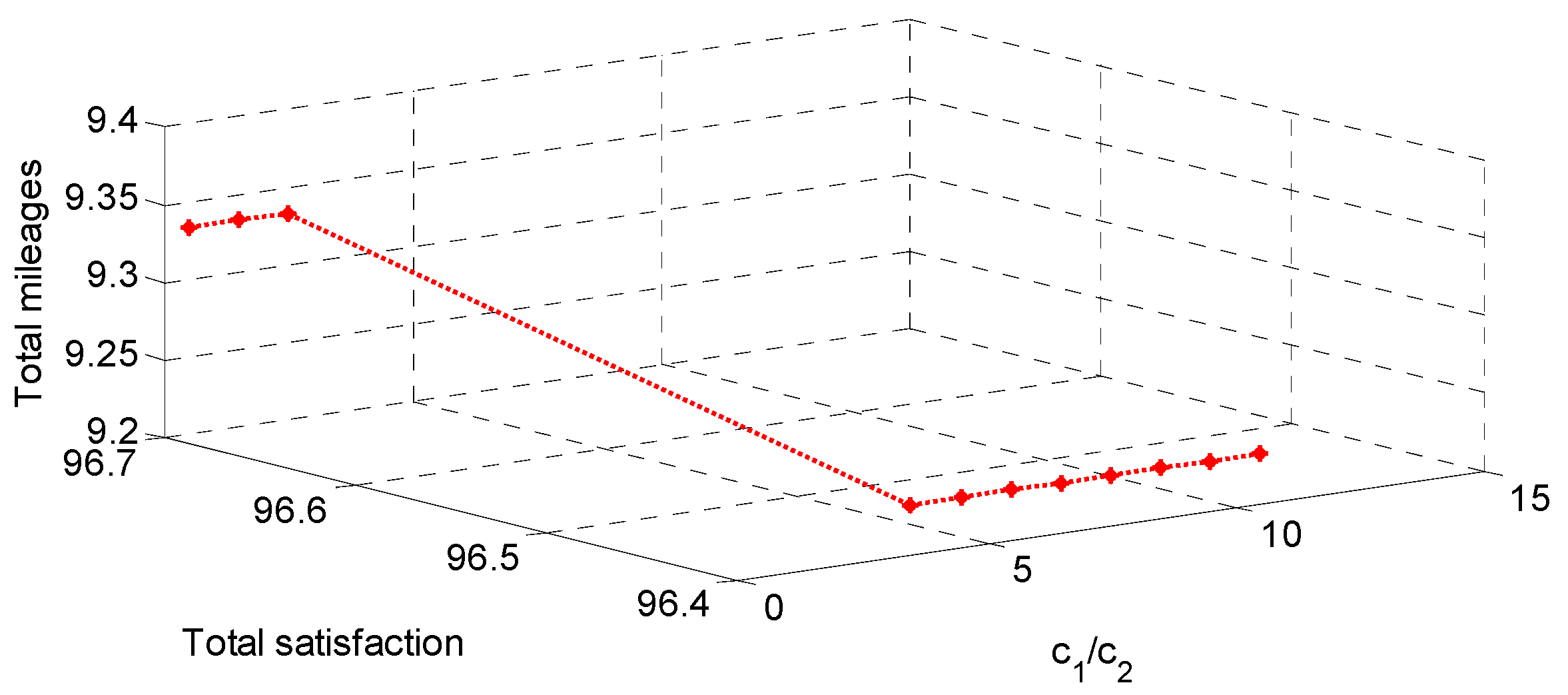
Furthermore, Figure 5 reveals how the changes of weight coefficient affect a trade-off between total mileage and the total average satisfied demand. As the target weight coefficient gradually increases, the change of the weight coefficient does not reach the critical value and the total mileage and the passenger satisfaction remain the same, except for = 3.5 changing the objective value at 0.1 km to be 0.3. When these changes happen, the scheduling objective focuses on sacrificing passenger satisfaction with a reduction in mileage.
Furthermore, the solutions of the improved BA are compared with the standard BA, standard GSO, and Cplex in order to verify the effectiveness. The results are shown in Table 6, from which we can see the following:
- (1)
- When the scale of the problem is small, all three heuristic algorithms can find the optimal solution. As the scale of the problem becomes larger, the quality of the solutions worsens.
- (2)
- The quality and the robustness of the improved BA are better than those of the standard BA and GSO. This shows that there is effective improvement of the algorithm when introducing the idea that GSO’s “small part-segmented rogues walk at random” into standard BA to improve the speed and position updates in the formulas of bats, which can maintain the diversity of groups.
6. Conclusions
This paper presents a novel optimization methodology for DRT with multiple time windows to reveal the relationship between the total mileage and passenger satisfaction. Being different from existing studies, the proposed methodology has the ability to (1) offer an interactive process for designing feeder transit routing and guiding the passenger to choose a best boarding time window; and (2) develop a hybrid algorithm combining BA and GSO to efficiently yield the acceptable solution to the proposed model. The feasibility and applicability of the proposed model is illustrated with a real-world example solved in terms of optimality. Results show that the total mileage of this model is significantly reduced by 15.2%, while the total satisfaction is significantly increased by 7.1%, compared with the traditional DRT model. With an increase in the number of vehicles, both total satisfaction and mileage slightly increased. Furthermore, the difference in optimal solutions between different heuristic algorithms and the use of Cplex is about 0–20%, but the calculation time is within an acceptable range. This proves the validity of the proposed algorithm.
It is important to note that this work is based on a hypothesis of pedestrian boarding places such as bus stops and neglected the integrated operation of pedestrian guidance (from home addresses to candidate bus stops). In this sense, the design of the feeder bus network should take the interactions between passenger walking distances and buses’ operational costs into account. As a result, extending the model to simultaneously select bus stops and assign pedestrians to the stops is a worthwhile direction for further work and research.
Acknowledgments
This paper is funded by Jiangsu provincial government scholarship program;the National Natural Science Foundation of China (61503201); Natural Science Foundation of the Jiangsu Province in China (BK20161280); the Humanities and Social Sciences Foundation of the Ministry of Education in China(16YJCZH086);Natural Science Foundation of the Jiangsu High Education (17KJB520029); Nantong Science and Technology Innovation Program (GY12016020,GY12016019); the Science and Technology Key Research and Development Project of Huai’an City (HAS2015015);the open fund for the Key Laboratory for traffic and transportation security of Jiangsu Province (TTS2016-01); Nantong University-Nantong Joint Research Center for Intelligent Information Technology (KFKT2017B08);Project of excellent graduate innovation in Hebei Province(2016348).
Author Contributions
Bo Sun wrote the manuscript; Bo Sun and Ming Wei provided relevant information, discussed the data, and corrected the manuscript; and Senlai Zhu revised the manuscript. All authors have read and approved the final manuscript. All authors would also like to thank Tao Liu for his advice on this paper.
Conflicts of Interest
The authors declare no conflict of interest.
References
- Ceder, A. Stepwise multi-criteria and multi-strategy design of public transit shuttles. J. Multi-Criteria Decis. Anal. 2009, 16, 21–38. [Google Scholar] [CrossRef]
- Wei, M.; Sun, B. Bi-level programming model for multi-modal regional bus timetable and vehicle dispatch with stochastic travel time. Clust. Comput. 2017, 20, 401–411. [Google Scholar] [CrossRef]
- Savelsbergh, A.L.M. An extended demand responsive connector. EURO J. Transp. Logist. 2017, 6, 25–50. [Google Scholar]
- Shen, J.X.; Yang, S.Q.; Gao, X.M.; Qiu, F. Vehicle routing and scheduling of demand-responsive connector with on-demand stations. Adv. Mech. Eng. 2017, 9, 1–10. [Google Scholar] [CrossRef]
- Daniela, F.; Elena, M.; Paola, P. Ant colony system for a VRP with multiple time windows and multiple visits. J. Interdiscipl. Math. 2007, 10, 263–284. [Google Scholar]
- Belhaiza, S.; Hansen, P.; Laporte, G. A hybrid variable neighborhood tabu search heuristic for the vehicle routing problem with multiple time windows. Comput. Oper. Res. 2014, 52, 269–281. [Google Scholar] [CrossRef]
- Maral, S.; Saeed, K.; Iraj, M.; Nezam, M.A. A partial delivery bi-objective vehicle routing model with time windows and customer satisfaction function. Mediterr. J. Soc. Sci. 2016, 7, 101–111. [Google Scholar]
- Azi, N.; Gendreau, M.; Potvin, J.Y. An exact algorithm for a single-vehicle routing problem with time windows and multiple routes. Eur. J. Oper. Res. 2007, 178, 755–766. [Google Scholar] [CrossRef]
- Savelsbergh, M.W.P.; Sol, M. The general pickup and delivery problem. Transp. Sci. 1995, 29, 17–29. [Google Scholar] [CrossRef]
- Desaulniers, G.; Desrosiers, J.; Erdmann, A.; Solomon, M.M.; Soumis, F. VRP with pickup and delivery. In The Vehicle Routing Problem; SIAM Monographs on Discrete Mathematics and Applications; Toth, P., Vigo, D., Eds.; Society for Industrial and Applied Mathematics: Philadelphia, PA, USA, 2002. [Google Scholar]
- Cordeau, J.F.; Laporte, G. The dial-a-ride problem: Models and algorithms. Ann. Oper. Res. 2007, 153, 29–46. [Google Scholar] [CrossRef]
- Laporte, G. Fifty years of vehicle routing. Transp. Sci. 2009, 43, 408–416. [Google Scholar] [CrossRef]
- Parragh, S.N.; Doerner, K.F.; Hartl, R.F. A survey on pickup and delivery problems. J. FürBetriebswirtschaft 2008, 58, 21–51. [Google Scholar] [CrossRef]
- Cordeau, J.; Laporte, G.; Potvin, J.Y.; Savelsbergh, M.W. Chapter 7 transportation on demand. In Transportation, Handbooks in Operations Research and Management Science; Barnhart, C., Laporte, G., Eds.; Elsevier: Amsterdam, The Netherlands, 2007; Volume 14, pp. 429–466. [Google Scholar]
- Quadrifoglio, L.; Li, X. A methodology to derive the critical demand density for designing and operating feeder transit services. Transp. Res. Part B 2009, 43, 922–935. [Google Scholar] [CrossRef]
- Hashimoto, H.; Yagiura, M.; Imahori, S.; Ibaraki, T. Recent progress of local search in handling the time window constraints of the vehicle routing problem. Ann. Oper. Res. 2013, 204, 171–187. [Google Scholar] [CrossRef]
- Taillard, E.D.; Laporte, G.; Gendreau, M. Vehicle routing with multiple use of vehicles. J. Oper. Res. Soc. 1996, 47, 1065–1070. [Google Scholar] [CrossRef]
- Azi, N.; Gendreau, M.; Potvin, J.Y. An exact algorithm for a vehicle routing problem with time windows and multiple use of vehicles. Eur. J. Oper. Res. 2010, 202, 756–763. [Google Scholar] [CrossRef]
- Polacek, M.; Hartl, R.F.; Doerner, K.; Reimann, M. A variable neighborhood search for the multi depot vehicle routing problem with time windows. J. Heuristics 2004, 10, 613–627. [Google Scholar] [CrossRef]
- Vidal, T.; Crainic, T.; Gendreau, M.; Lahrichi, N.; Rei, W. A hybrid genetic algorithm for multidepot and periodic vehicle routing problems. Oper. Res. 2012, 60, 611–624. [Google Scholar] [CrossRef]
- Sevilla, F.C.; de Blas, C.S. Vehicle Routing Problem with Time Windows and Intermediate Facilities; SEIO 003 Edicions de la Universitat de Lleida; Universitat de Lleida: Lleida, Spain, 2003; pp. 3088–3096. [Google Scholar]
- Jerby, S.; Ceder, A. Optimal routing design for shuttle bus service. Transp. Res. Rec. 2006, 1971, 14–22. [Google Scholar] [CrossRef]
- Sun, Y.; Sun, X.; Li, B.; Gao, D. Joint optimization of a rail transit route and bus routes in a transit corridor. Procedia-Soc. Behav. Sci. 2013, 96, 1218–1226. [Google Scholar] [CrossRef]
- Szeto, W.; Jiang, Y. Transit route and frequency design: Bi-level modeling and hybrid artificial bee colony algorithm approach. Transp. Res. Part B 2014, 67, 235–263. [Google Scholar] [CrossRef] [Green Version]
- Yan, Y.; Liu, Z.; Meng, Q.; Jiang, Y. Robust optimization model of bus transit network design with stochastic travel time. J. Transp. Eng. 2013, 139, 625–634. [Google Scholar] [CrossRef]
- Chevrier, R.; Liefooghe, A.; Jourdan, L.; Dhaenens, C. Solving a dial-a-ride problem with a hybrid evolutionary multi-objective approach: Application to demand responsive transport. Appl. Soft Comput. 2012, 12, 1247–1258. [Google Scholar] [CrossRef]
- Zhu, Z.; Guo, X.; Zeng, J.; Zhang, S. Route Design Model of Feeder Bus Service for Urban Rail Transit Stations. Math. Probl. Eng. 2017, 1–6. [Google Scholar] [CrossRef]
- Lu, X.; Yu, J.; Yang, X.; Pan, S.; Zou, N. Flexible feeder transit route design to enhance service accessibility in urban area. J. Adv. Transp. 2016, 50, 507–521. [Google Scholar] [CrossRef]
- Calvete, H.I.; Galé, C.; Oliveros, M.J.; Sánchez-Valverde, B. A goal programming approach to vehicle routing problems with soft time windows. Eur. J. Oper. Res. 2007, 177, 1720–1733. [Google Scholar] [CrossRef]
- El-Sherbeny, N.A. Vehicle routing with time windows: An overview of exact, heuristic and metaheuristic methods. J. King Saud Univ.-Sci. 2010, 22, 123–131. [Google Scholar] [CrossRef]
- Repoussis, P.P.; Tarantilis, C.D. Solving the fleet size and mix vehicle routing problem with time windows via adaptive memory programming. Transp. Res. Part C Emerg. Technol. 2010, 18, 695–712. [Google Scholar] [CrossRef]
- Potvin, J.Y.; Bengio, S. The vehicle routing problem with time windows part II: Genetic search. Inf. J. Comput. 1996, 8, 165–172. [Google Scholar] [CrossRef]
- Kim, M.; Schonfeld, P. Integrating bus services with mixed fleets. Transp. Res. Part B 2013, 55, 227–244. [Google Scholar] [CrossRef]
- Carotenuto, P.; Storchi, G. Hybrid genetic algorithm to approach the DaRP in a demand responsive passenger service. IFAC Proc. Vol. 2006, 39, 315–320. [Google Scholar] [CrossRef]
- Ali, B.; Mahdi, B.; Fahime, Z. Two phase genetic algorithm for vehicle routing and scheduling problem with cross-docking and time windows considering customer satisfaction. J. Ind. Eng. Int. 2017, 17, 1–16. [Google Scholar]
- Fan, W.; Machemehl, R.B. Tabu search strategies for the public transportation network optimizations with variable transit demand. Comput.-Aided Civ. Infrastruct. Eng. 2008, 23, 502–520. [Google Scholar] [CrossRef]
- Crainic, T.G.; Malucelli, F.; Nonato, M. Meta-Heuristics for a Class of Demand-Responsive Transit Systems. Inf. J. Comput. 2005, 17, 10–24. [Google Scholar] [CrossRef]
- Fisher, M.; Jornsteen, K.; Madsen, O. Vehicle routing with time windows: Two optimization algorithms. Oper. Res. 1997, 45, 488–492. [Google Scholar] [CrossRef]
- Schulze, J.; Fahle, T. A parallel algorithm for the vehicle routing problem with time windows constraints. Ann. Oper. Res. 1999, 86, 585–607. [Google Scholar] [CrossRef]
- Wu, J.; Lederer, A. A meta-analysis of the role of environment-based voluntariness in information technology acceptance. MIS Q. 2009, 33, 419–432. [Google Scholar] [CrossRef]
- Chen, C.F.; Xu, X.; Arpan, L. Between the technology acceptance model and sustainable energy technology acceptance model: Investigating smart meter acceptance in the United States. Energy Res. Soc. Sci. 2017, 25, 93–104. [Google Scholar] [CrossRef]
- Chakri, A.; Khelif, R.; Benouaret, M.; Yang, X.S. New directional bat algorithm for continuous optimization problems. Expert Syst. Appl. 2017, 69, 159–175. [Google Scholar] [CrossRef]
- Olivas, F.; Amador-Angulo, L.; Perez, J.; Caraveo, C.; Valdez, F.; Castillo, O. Comparative Study of Type-2 Fuzzy Particle Swarm, Bee Colony and Bat Algorithms in Optimization of Fuzzy Controllers. Algorithms 2017, 10, 101. [Google Scholar] [CrossRef]
- Wang, L.; Zhong, X.; Liu, M. A novel group search optimizer for multi-objective optimization. Expert Syst. Appl. 2012, 39, 2939–2946. [Google Scholar] [CrossRef]
- Wei, M.; Chen, X.W.; Sun, B. Model and algorithm for resolving regional bus scheduling problems with fuzzy travel times. J. Intell. Fuzzy Syst. 2015, 29, 2689–2696. [Google Scholar] [CrossRef]
Figure 1.
Research Framework.
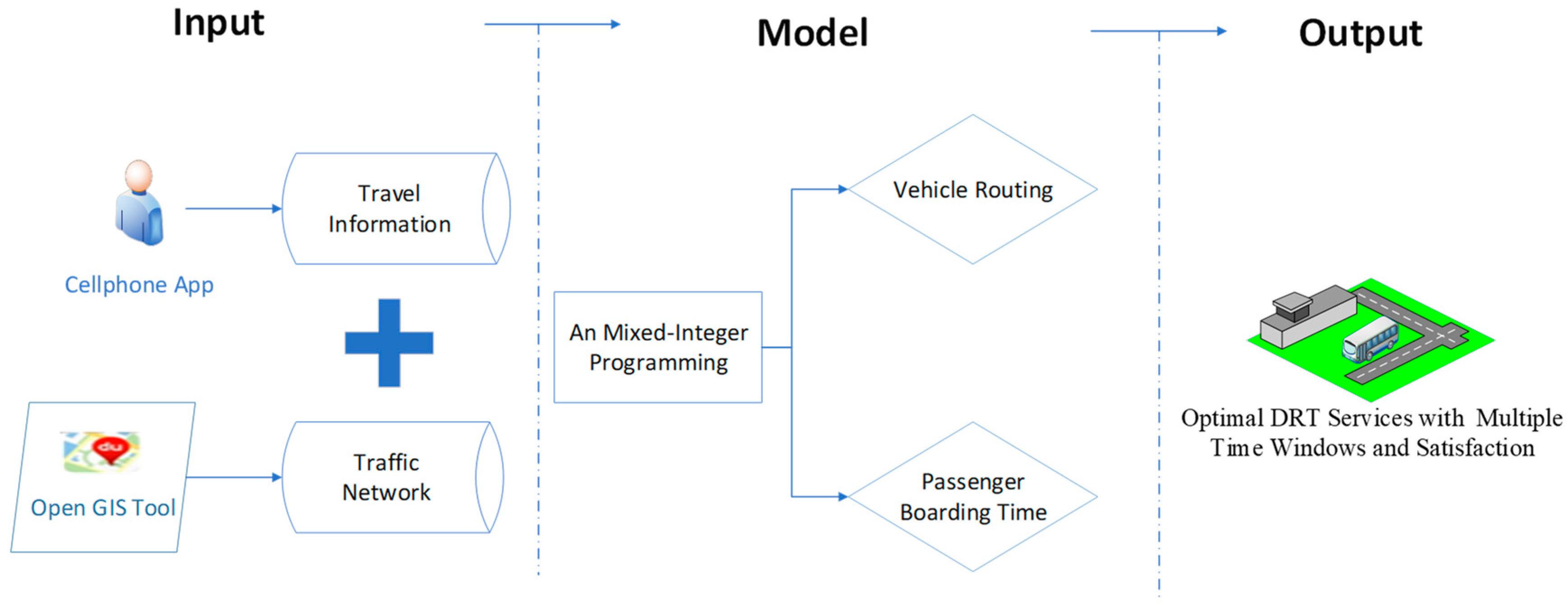
Figure 2.
Graphical representation of the integrated DRT problem.

Figure 3.
Spatial distribution of vehicle visiting points (Map resource: Baidu).
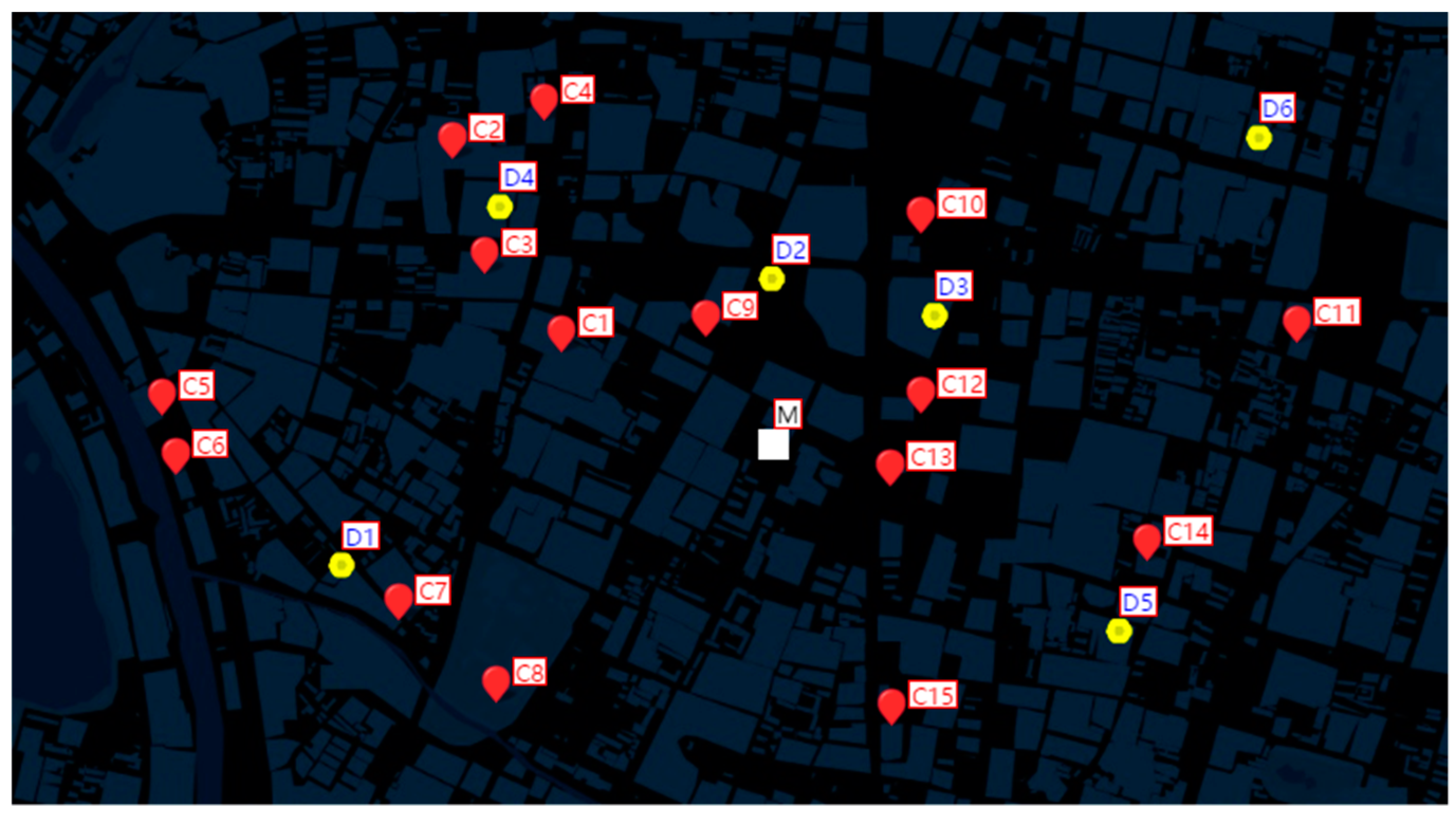
Figure 4.
Result comparison of proposed model and traditional DRTs.

Figure 5.
Influence of weight coefficient on the scheduling result.

Table 1.
Parameters and variables in the mathematical model.
| Indices | |
| Vehicular node (demand point, dispatch center, and urban rail station) index | |
| Vehicle index | |
| Time window | |
| Sets | |
| Set of demand points | |
| Set of vehicles | |
| Set of dispatch centers | |
| Set of rail transit stations | |
| Parameters | |
| Number of passengers at the demand point ; | |
| The hth travel time window of the demand point ; | |
| The maximum expected ride time of the demand point ; | |
| The minimum expected ride time of the demand point ; | |
| Q | Maximum capacity of the vehicle |
| Maximum length of the vehicle | |
| Minimum travel time of feeder bus route | |
| Distance from the vehicular node to the vehicular node ; | |
| Travel time from the vehicular node to the vehicular node ; | |
| The time of vehicle k arriving the rail transit stations | |
| The time of vehicle k arriving the demand point ; | |
| Number of passengers at customer point assigned to vehicle k; | |
| A function to calculate the passenger satisfaction at demand point based on his/her ride time ; , | |
| Operational cost yuan/km | |
| Satisfaction cost yuan/person | |
| A very large fixed value | |
| Decision Variables | |
| Whether the vehicular node precedes the vehicular node on the vehicle k, or not; , | |
| Whether the vehicular node is covered by the vehicle k, or not; , | |
| An auxiliary (real) variable for sub-tour elimination constraint in vehicle k; | |
Table 2.
Basic information of demand points.
| No. | ||||
|---|---|---|---|---|
| C1 | [8:10–8:20], [8:00–8:33] | 5 | 15 | 3 |
| C2 | [8:00–8:10], [8:20–8:30] | 10 | 20 | 1 |
| C3 | [8:10–8:20], [10:05–10:15] | 5 | 15 | 1 |
| C4 | 8:15–8:25 | 5 | 10 | 2 |
| C5 | 8:15–8:25 | 5 | 20 | 2 |
| C6 | 8:20–8:30 | 10 | 20 | 3 |
| C7 | [8:05–8:15], [8:20–8:30] | 10 | 20 | 4 |
| C8 | 8:08–8:18 | 10 | 20 | 1 |
| C9 | 8:10–8:20 | 5 | 15 | 2 |
| C10 | [8:05–8:15], [8:10–8:20], [8:35–8:45] | 5 | 15 | 2 |
| C11 | 8:20–8:30 | 5 | 15 | 4 |
| C12 | [8:10–8:20], [8:25–8:35] | 5 | 20 | 1 |
| C13 | 8:00–8:10 | 5 | 20 | 3 |
| C14 | 8:10–8:20 | 5 | 20 | 1 |
| C15 | 8:20–8:30 | 5 | 20 | 12 |
Table 3.
Assignment result of passengers picked up by vehicles.
| Demand Point | Boarding Time | Ride Time | Satisfaction | Vehicle |
|---|---|---|---|---|
| C5 | 8:17 | 10.2 | 0.65 | V1 |
| C6 | 8:18 | 9.7 | 1 | |
| C7 | 8:20 | 7.3 | 1 | |
| C8 | 8:21 | 6.2 | 1 | |
| C15 | 8:25 | 2.7 | 1 | |
| C10 | 8:27 | 2.3 | 1 | V2 |
| C11 | 8:22 | 7.3 | 0.77 | |
| C12 | 8:25 | 3.9 | 1 | |
| C14 | 8:20 | 9.6 | 0.69 | |
| C1 | 8:13 | 2.4 | 1 | V3 |
| C2 | 8:10 | 5.7 | 1 | |
| C3 | 8:12 | 3.4 | 1 | |
| C4 | 8:11 | 4.8 | 1 | |
| C9 | 8:15 | 1.1 | 1 | |
| C13 | 8:05 | 10.5 | 0.63 |
Table 4.
Routing and scheduling plan of each vehicle.
| Vehicle | The Sequence of Demand Points Visited by Vehicle | Travel Distance (km) | Travel Time (min) | Number of Passengers |
|---|---|---|---|---|
| V1 | D1(8:15)–C5(8:17)–C6(8:18)–C7(8:20)–C8(8:21)–C15(8:25)–M (8:27) | 3.1 | 12.2 | 12 |
| V2 | D4(8:17)–C14(8:20)–C11(8:22)–C12(8:25)–C10(8:27)–M(6:29) | 3.1 | 12.5 | 8 |
| V3 | D4(8:03)–C13(8:05)–C2(8:10)–C4(8:11)–C3(8:12)–C1(8:13)–C9(8:15)–M(8:16) | 3.0 | 12.1 | 12 |
Table 5.
Comparison of model and algorithm performance among three scenarios.
| Scenario | Objective (yuan) | Total Satisfaction | Total Mileage (km) | Total Time (min) |
|---|---|---|---|---|
| 3 Vehicles | −36.4 | 96.4 | 9.2 | 36.8 |
| 4 Vehicles | −52.1 | 130.9 | 12.1 | 49.4 |
| 5 Vehicles | −68.4 | 157.4 | 13.7 | 57.6 |
Table 6.
Comparison of different algorithms.
| Number of Demand Points | Cplex | Improved BA | Standard BA | Standard GSO | ||||
|---|---|---|---|---|---|---|---|---|
| Best Solution (yuan) | Probability | Best Solution (yuan) | Probability | Best Solution (yuan) | Probability | Best Solution (yuan) | Probability | |
| 15 | −36.4 | 100% | −36.4 | 86.7% | −36.4 | 74.7% | −36.4 | 73.4% |
| 30 | −41.8 | 100% | −40.6 | 77.1% | −38.8 | 65.2% | −37.7 | 62.8% |
| 60 | −76.5 | 100% | −69.9 | 62.3% | −63.3 | 51.8% | −61.5 | 47.6% |
© 2018 by the authors. Licensee MDPI, Basel, Switzerland. This article is an open access article distributed under the terms and conditions of the Creative Commons Attribution (CC BY) license (http://creativecommons.org/licenses/by/4.0/).
Share and Cite
MDPI and ACS Style
Sun, B.; Wei, M.; Zhu, S. Optimal Design of Demand-Responsive Feeder Transit Services with Passengers’ Multiple Time Windows and Satisfaction. Future Internet 2018, 10, 30. https://doi.org/10.3390/fi10030030
AMA Style
Sun B, Wei M, Zhu S. Optimal Design of Demand-Responsive Feeder Transit Services with Passengers’ Multiple Time Windows and Satisfaction. Future Internet. 2018; 10(3):30. https://doi.org/10.3390/fi10030030
Chicago/Turabian StyleSun, Bo, Ming Wei, and Senlai Zhu. 2018. "Optimal Design of Demand-Responsive Feeder Transit Services with Passengers’ Multiple Time Windows and Satisfaction" Future Internet 10, no. 3: 30. https://doi.org/10.3390/fi10030030
Note that from the first issue of 2016, this journal uses article numbers instead of page numbers. See further details here.