Network Measurement and Performance Analysis at Server Side


Department of Computer Science and Engineering, Shanghai Jiao Tong University, Shanghai 200240, China
*
Author to whom correspondence should be addressed.
Future Internet 2018, 10(7), 67; https://doi.org/10.3390/fi10070067
Submission received: 14 June 2018
/
Revised: 13 July 2018
/
Accepted: 13 July 2018
/
Published: 16 July 2018
Abstract
:Network performance diagnostics is an important topic that has been studied since the Internet was invented. However, it remains a challenging task, while the network evolves and becomes more and more complicated over time. One of the main challenges is that all network components (e.g., senders, receivers, and relay nodes) make decision based only on local information and they are all likely to be performance bottlenecks. Although Software Defined Networking (SDN) proposes to embrace a centralize network intelligence for a better control, the cost to collect complete network states in packet level is not affordable in terms of collection latency, bandwidth, and processing power. With the emergence of the new types of networks (e.g., Internet of Everything, Mission-Critical Control, data-intensive mobile apps, etc.), the network demands are getting more diverse. It is critical to provide finer granularity and real-time diagnostics to serve various demands. In this paper, we present EVA, a network performance analysis tool that guides developers and network operators to fix problems in a timely manner. EVA passively collects packet traces near the server (hypervisor, NIC, or top-of-rack switch), and pinpoints the location of the performance bottleneck (sender, network, or receiver). EVA works without detailed knowledge of application or network stack and is therefore easy to deploy. We use three types of real-world network datasets and perform trace-driven experiments to demonstrate EVA’s accuracy and generality. We also present the problems observed in these datasets by applying EVA.
1. Introduction
With increasing network capacity and machine processing power, network applications should have higher throughput and lower latency. However, these applications still sometimes experience performance degradation. Performance problems can be caused by any of a number of factors. Examples include client sends zero window due to the inability to buffer more data, application cannot generate enough data to fill the network, network congestion, bufferbloat [1], limited bandwidth of bottleneck link, etc. Troubleshooting these problems is challenging, mainly because the server, network, and client make decision based on the local information they observe, and all of them are likely to be performance bottlenecks. Specifically, for clients, delayed acknowledgments may introduce unexpected latency, especially for interactive applications; limited receive buffer can significantly reduce throughput. For networks, congestion and bufferbloat may occur at any link along the path. For servers, things become even more complicated. For example, application developers may ignore Nagle’s algorithm [2] and forget to turn on TCP_NODELAY option. As a result, a temporary form of deadlock may occur due to the interaction between the Nagle’s algorithm and delayed acknowledgments. However, even with perfect interaction between application and network stack, TCP’s congestion control may still fail to fully utilize network bandwidth [1,3]. More importantly, today’s network applications adopt multi-tier architectures, which consist of user-facing front-end (e.g., reverse proxy and load balancer) and IO/CPU-intensive back-end (e.g., database query). Problems with any of these components can affect user-perceived performance. Developers sometimes blame “the network” for problems they cannot diagnose; in turn, the network operators blame the developers if the network shows no signs of equipment failure or persistent congestion. As a result, identifying the entity responsible for poor performance is often the most time-consuming and expensive part of failure detection and can take from an hour to days in data centers [4]. Fortunately, once the location of the problem is correctly identified, specialized tools within that component can pinpoint and fix the problem.
Existing solutions such as fine-grain packet monitoring or profiling of the end-host network stack almost all work under the assumption that the TCP congestion control is not the one to blame. Furthermore, nearly all packet monitoring tools measure the network conditions (congestion, available bandwidth, etc.) by inferring end-hosts’ congestion control status. Such approach may fail for two reasons: First, today TCP’s loss-based congestion control, even with the current best of breed, Cubic [5], experience pool performance in some scenarios [3]. Second, one congestion control algorithm may work quite differently from another, e.g., loss-based Cubic and delay-based Vegas. As a result, we argue that network conditions should be treated independently of TCP congestion control status, thus should be measured directly from packet traces.
In this paper, we present EVA, a network measurement and performance analysis tool that enables network operators and application developers to detect and diagnose network performance problems. Given the complexity network performance problems, we cannot hope EVA fully automates the detection, diagnosis, and repair of network performance problems. Instead, our goal is reducing the demand for developer time by automatically identifying performance problems and narrowing them down to specific times and locations. To achieve this goal, EVA continuously monitors bidirectional packet headers near the server, infers essential metrics of both network and end-hosts, and detects the performance bottleneck in a timely manner. In particular, EVA measures RTprop (round-trip propagation time) and BtlBw (bottleneck bandwidth) of a TCP flow that represent network conditions. The two metrics enable us to pinpoint the locations of the problems, especially congestion control. Compared with similar tools, the following advantages of EVA make it a viable or even better solution:
- Generic: Our solution neither relies on detailed knowledge of application nor congestion control. In fact, server side bidirectional packet traces are the only input of EVA.
- Real-time: Our tool measures the network and pinpoints performance problems in a real-time manner (offline analysis also supported). Owing to multithreaded implementation and PF_RING [6] accelerated packet capture, EVA achieves 2.26 Mpps (packet per second) speed on commodity server equipped with 10 Gbps NIC.
- Accurate: In our experiments, EVA successfully identifies almost all the performance problems, which means it has a high diagnostic accuracy.
We used EVA to diagnose three real-world datasets: user-facing CDN traffic of a famous cloud computing company in China, traffic of a campus website, and P2P traffic over campus networks. Based on the analysis results, we not only pinpoint the performance limitations, but also propose possible solutions.
Our major contributions include the following. First, we designed a novel approach to measure network conditions based on packet traces. This approach is independent of application and work for any congestion control algorithm. Second, we implemented a generic and high-speed network performance analysis tool, EVA, which can detect performance problems in a timely manner. Third, we used the tool to diagnose real-world traffic and showed our key observations.
The rest of this paper is organized as follows. Section 2 summarizes the related work. Section 3 explains the measurement methodology. Section 4 describes the datasets. Section 5 describes our efforts to validate EVA’s performance. Section 6 shows the results of applying it to the datasets. Section 7 concludes the paper.
2. Related Work
We discuss the existing work related to network performance measurement in the following categories:
Packet level analysis. Several tools analyze packet traces to find performance bottlenecks. T-RAT [7] analyzes packet traces collected at core routers and outputs diagnostic results similar to EVA. However, T-RAT does not consider congestion control variations and therefore lacks generality. Our work can be seen as an extension of T-RAT in modern network environments. Everflow [8] collects packet-level information in large datacenter networks for scalable and flexible access. However, it relies on “match and mirror” functionality of commodity switches, and our solution does not. Other tools measure wireless network performance [9,10,11,12]. Benko et al. [9] passively monitored GPRS network performance by analyzing TCP packets at the ingress/egress router interface. Sundaresan S. [10] monitored home wireless network performance in the home wireless access point. Botta et al. [11], Ricciato [12] measured the performance of mobile networks, but the goals are different. Botta et al. [11] focused on heavy-users in 3G networks and Ricciato [12] monitored network traffic to optimize the 3G networks.
Instrumenting the network stack. Monitoring the network stack is more lightweight comparing to our packet-level approach. In particular, TCP states and application behaviors can be observed at very low cost. SNAP [13] pinpoints performance problems similarly to EVA. However, it leverages TCP statistics (number of bytes in the send buffer, total number of fast retransmissions, etc.) and socket-level logs (the time and number of bytes whenever the socket makes a read/write call) in network stack. Similarly, NetPoirot [4] collects TCP statistics at each machine’s hypervisor or within individual VMs to identify root causes of failures. Comparing to EVA, these tools are too intrusive since they must run inside the server.
Measurement in switches. Some tools uses flow-level information (NetFlow [14] and sFlow [15]) collected on switches to provide support for different measurement tasks. However, flow-level information cannot provide good fidelity comparing to our fine-grain packet monitoring. As an alternative, many sketch-based streaming algorithms have been proposed [16,17,18,19]. However, these algorithms are tightly coupled to the intended metric of interest, forcing vendors to invest time and effort in building specialized hardware. In contrast, our solution is software-only and thus more generic. In addition, compared to our end-hosts approach, monitoring in switches provides more visibility but limited support for measurement (i.e., programmability and processing power). Therefore, various query languages [20,21,22] and switch hardware [22] have been proposed. As an alternative, SwitchPointer [23] combines the advantages of both, i.e., resources and programmability of end-hosts and network visibility of switches. EVA does not use network visibility of switches; instead, it abstracts any arbitrarily complex path into a single link with the same propagation delay and bottleneck rate.
Measurement in mobile devices. To monitor mobile network performance, an promising approach is to use smartphone apps [24,25,26,27]. These tools focus on wireless network (3G/4G, WiFi) and mobile devices performance. 4GTest [25] is a network performance measurement app with distributed server support globally. It actively measures the network RTT and throughput. There are two main differences between 4GTest and EVA. First, EVA runs near the server, and it pays more attention to the server side performance. Second, EVA measures network conditions passively, while 4GTest takes a active approach.
Other performance measurement solutions. Several works analyze network performance in different ways. Nguyen et al. [28] measured TCP end-to-end performance in a simulated mobile network. They focused on the interactions between the mobile network architecture and TCP. MagNets [29,30] is a novel wireless access network testbed where traffic is created by real users with real applications. The testbed is able to evaluate the impacts of wireless network setup (link characteristics, topology, etc.) on network performance. These solutions do not analyze packets as EVA does, but measure network performance directly in experimental environments.
3. Measurement Methodology
EVA leverages network path properties and common principles underlying various TCP flavors. In particular, it passively measures RTprop and BtlBw for each TCP flow, groups packets into flights, and identifies performance bottlenecks of each flight. Before describing how EVA works in detail, we first specify the requirements that motivate its design. These include the range of performance problems it needs to identify as well as the environment in which we want to use it.
The performance of a TCP flow is determined by several factors. We characterize the possible limiting factors as follows:
- Slow start limited. TCP flow is slow starting, thus unable to make full use of network resources. Some flows may never leave slow start (i.e., short-lived connection), while others may enter slow start stage multiple times (e.g., after timeout retransmission).
- Application limited. The sender application does not generate enough data to fill the network. This situation will appear in a variety of scenarios, e.g., a ssh server can send a single short packet in one flight. It is worth noting that an idle connection should also be treated as application limited.
- Send buffer limited. The network stack allocates a send buffer for each TCP connection to manage in flight data (i.e., data that have sent but not acknowledged). Sender cannot fill the network if this buffer is too small.
- Congestion control limited. Some congestion controls may underestimate network capacity in certain situations. For example, when bottleneck buffers are small, loss-based congestion control misinterprets loss as a signal of congestion, leading to low throughput.
- Receive window limited. The network stack allocates a receive buffer for each TCP connection to manage data received but not retrieved by the application. Small receive buffer can limit the send rate. This happens when the application sets a small fixed receive buffer or retrieves data from the network stack slower than transport layer receives the data. It is worth noting that a zero window may be advertised, forcing the sender to stop immediately.
- Bandwidth limited. The sender fully utilizes, and is limited by, the bandwidth on the bottleneck link.
- Congestion limited. The network is congested, i.e., data packets are suffering loss and high latency. This definition is independent of congestion control, whether it is loss-based or delay-based.
- Bufferbloat limited. Bufferbloat is the undesirable latency that comes from a router or other network equipment buffering too much data. For example, when bottleneck buffers are large, loss-based congestion control keeps them full, causing bufferbloat.
In addition to the above functionality, we have the following requirements for EVA. First, to maximize the scope of application, it must be compatible with different congestion controls, that is, it cannot rely on specific congestion control behaviors. Second, to deal with large (even infinite) network traffic, it must run continuously with limited CPU and memory resources, thus it must analysis in a streaming fashion. Finally, to deal with long-lived TCP connections, SYN and SYN-ACK are not necessary, which means it can start from the middle of a flow.
To meet the above requirements, we divide EVA into three components:
- The RTprop estimator continuously estimates RTprop for a TCP flow.
- The BtlBw estimator continuously estimates BtlBw for a TCP flow.
- Performance analysis first groups packets into flights, and then analyzes performance problems for each flight.
In addition, since EVA is deployed near the server side (hypervisor, NIC, or top-of-rack switch), it can not only see bidirectional packet traces, but also measure end-to-end metrics from the end-host perspective. We utilize the two properties to simplify implementation of EVA. Next, we detail the implementation of the three key components.
3.1. BtlBw Estimator
For any network path at any time, there must be exactly one bottleneck router/switch, whose available bandwidth is the physical upper bound of data delivery rate of TCP flows that traverse the path. We define this available bandwidth as BtlBw, i.e., bottleneck bandwidth. BtlBw can be measured in network stack [3], however, we have to adopt a packet-based approach that is similar but somehow more challenging, since the application behavior and the congestion control status are invisible to us.
To estimate BtlBw, we continuously measure the rate that data are delivered to receiver. Note that delivery rate is different from send rate: the former is bound by BtlBw but the latter is not. When an ACK arrives back to the sender, it conveys two pieces of information: the amount of data delivered and the time elapsed since the corresponding data packet departed. The ratio of the two is the delivery rate. After obtaining a stream of delivery rate samples, we use a windowed maximum filter to estimate BtlBw, which is similar to [3], but our window is flight-based rather than time-based. We explain how to separate packets into flights in detail in later subsections. On the arrival of each ACK that belongs to nth flight , we define:
where is the window length of the filter, which is set to ten flights in the current implementation. However, not all ACK can be used to update BtlBw. Specifically, when TCP flow is sender or receiver limited, delivery rate samples will be obviously lower than BtlBw. To avoid underestimation of BtlBw, EVA pauses updates to BtlBw in such situations.
Now, we can see the dynamics of BtlBw estimator. Initially, the window is empty. After several flights of data transfer, the window is filled up, so we have an initial estimate of the BtlBw. If the BtlBw increases, we would see immediately that the delivery rate goes up. If the BtlBw decreases, it would take several flights to correct the BtlBw estimate.
Several refinements and extensions have been made so that we can estimate BtlBw more accurately and more efficiently using only packet traces. First, since it is physically impossible for data to be delivered faster than they are sent in a sustained fashion, when the estimator notices that the delivery rate for a flight is faster than the send rate for the flight, it filters out the implausible delivery rate by capping the rate sample to be no higher than the send rate. Second, if a packet retransmission just filled the “hole” in the TCP byte stream, implausible delivery rate can still be observed even filtered by send rate. This problem stems from TCP’s cumulative ack mechanism, which can be solved by TCP SACK option that selectively acknowledges data blocks after the “hole”, so that we can know the actual bytes acked. Finally, we implemented Kathleen Nichols’ algorithm for tracking the estimate of a stream of delivery rate samples.
3.2. RTprop Estimator
For any network path at any time, there must exist a RTprop (round-trip propagation delay), which is the physical lower bound of RTT (the time interval from sending a data packet until it is acknowledged) of the path. We estimate RTprop based on a stream of RTT samples. Remember that EVA collects packets near the server, so it can measure RTT from the end-host perspective. In the following, we first describe the measurement of RTT, then show how to infer RTprop from the RTT samples.
RTT is measured by network stack to determine RTO (retransmission timeout). However, EVA measures RTT for two other purposes: (1) to estimate RTprop; and (2) to estimate the queuing delay. Both are major sources of RTT. For the most part, the same considerations and mechanisms that apply to RTT estimation for the purposes of retransmission timeout calculations [31] apply to EVA RTT samples. Namely, EVA does not use RTT samples based on the transmission time of retransmitted packets, since these are ambiguous, and thus unreliable. In addition, EVA calculates RTT samples using both cumulative and selective acknowledgments. The only divergence from RTT estimation for RTO is in the case where a given acknowledgment ACKs more than one data packet. To be conservative and schedule long timeouts to avoid spurious retransmissions, the maximum among such potential RTT samples is typically used for computing retransmission timeouts; i.e., SRTT is typically calculated using the data packet with the earliest transmission time. By contrast, to gain more accurate estimation of RTprop, EVA uses the minimum among such potential RTT samples; i.e., EVA calculates the RTT using the data packet with the latest transmission time.
After obtaining a stream of RTT samples, we use a windowed minimal filter to estimate RTprop, which is similar to [3]. On the arrival of each ACK at time T, we define:
where is the window length of the filter, which is set to 10 s in the current implementation. Instead of saving thousands of RTT samples for each flow, EVA uses a lightweight approximation, as described in Algorithm 1. If no lower RTT is observed within 10 s, EVA will take the latest RTT as an estimate of RTprop.
| Algorithm 1: RTprop estimator. |
 |
3.3. Performance Analysis
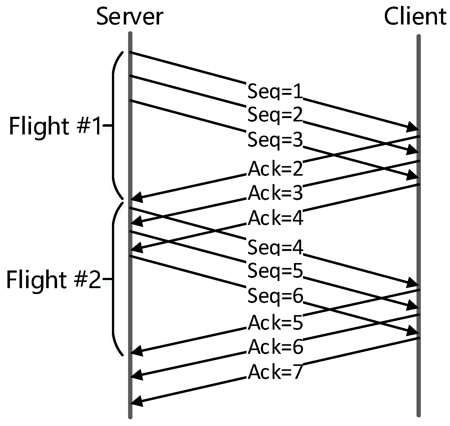
Based on the metrics inferred in above subsections, EVA analyzes the performance problems of TCP flows. Since the network conditions and state of sender and receiver can change over time, an analysis granularity is needed to track these changes. Existing work [7] adopts two kinds of approaches: fixed number of packets (e.g., 256 packets) or fixed time interval (e.g., 15 s). However, today’s network conditions have changed dramatically from a dozen years ago: NICs evolved from Mbps to Gbps and network latency can vary from less than one millisecond to hundreds of milliseconds. As a result, fixed granularity cannot adapt to such variations any more. Instead, EVA diagnoses performance problems per acknowledgment flight, as shown in Figure 1. In the following, we first show our method of grouping packets into flights, and then analyze performance bottlenecks for each flight. The latter is summarized in Table 1.
Flight size is the amount of data that have been sent but not yet acknowledged. It changes dynamically and is affected by many factors:
- When slow start limited, flight size increases exponentially.
- When application limited, flight size is the amount of data the application is willing to send.
- When receive window limited, flight size is bounded by receive window.
- When send buffer limited, flight size is bounded by send buffer size.
- Otherwise, flight size is determined by network and congestion control.
Since flight size is used to diagnose several TCP limiting factors, it must be measured continuously. Algorithm 2 shows EVA’s approach: It keeps track of data sequence from server and acknowledgment sequence from client, and then finds the boundary of each flight. The algorithm not only groups data sent, but also acknowledgments received.
| Algorithm 2: Group packets into flights. |
 |
Slow start limited. During slow start, the sender explores the bottleneck capacity exponentially, doubling the sending rate each round trip. To recognize this pattern, we test whether consecutive flight size fits the exponential relationship. If it is satisfied, this flight is considered slow start limited, otherwise the flow is considered to have left slow start. For a TCP flow that starts from the middle, we assume that its first flight is in a slow start stage, and, if not, it will quit on the next flight (exponential relationship is not satisfied).
Receive window limited. A TCP flow is considered receive window limited if the window clamps a flight size. Specifically, for each flight f, we calculate:
If , the flight is considered receive window limited. For a TCP flow that has just started from the middle, we may get the wrong result since window scale option has not converged yet. It is worth noting that the delivery rate collected by this flight will not be used to update BtlBw.
Congestion limited. We use the following three conditions to determine congestion limited:
- Packet retransmissions are seen in current flight.
- At least one RTT sample is larger than .
- The flight is not slow start limited or receive window limited.
Send buffer limited. The send buffer in network stack can clamp the flight size if it is too small. A flight is considered send buffer limited if all three of the following conditions are met:
- The flight size .
- The flight size and remains unchanged for at least three flights.
- The flight is not limited by slow start, receive window or network congestion.
The first condition ensures that the network is unsaturated (i.e., flight size is less than network BDP). The second condition ensures that the flight size is fixed by send buffer. The flight size is required to be at least one MSS, since a send buffer less than one MSS is impractical in real world.
Application limited. Interactive applications (SSH, HTTP, etc.) might not generate data fast enough to fill the network. A flight is considered application limited if the following conditions are met:
- The flight size .
- The flight contains at least one less-MSS-sized packet.
- The flight is not slow start limited, receive window limited, congestion limited or send buffer limited.
It is worth noting that we cannot just make a conclusion based on the second condition, since a fixed small send buffer may also introduce less-MSS-sized packets.
Congestion control limited. A flight is deemed congestion control limited if the size , and is not limited by above factors.
Bandwidth limited. A flight is considered bandwidth limited if more than half of the delivery rate samples in the flight are large than .
Bufferbloat limited. The flight is determined to be bufferbloat limited if all the RTT samples are larger than . Note that bufferbloat is independent of all the limitations above since it focuses on delay rather than throughput.
4. Datasets
We used packet traces from three sources in our study. The first packet trace was collected on a CDN server of UCloud [32] that delivered files to end users. Most contents the server delivered were small images and videos. Besides, the server ran Nginx [33] and Linux OS with an optimized congestion control algorithm and we did not know its details. The second packet trace was collected on a user-facing reverse proxy (Nginx) of a campus website. The site provided static page access and file download. Besides, the server ran Linux OS with Cubic congestion control. The last packet trace was collected on a P2P server (Transmission [34]) of campus network, which shared video contents among students. Note that the server shared only a few videos and the video size varied from 5 GB to 10 GB. The server ran Linux OS and BBR congestion control. All of the packet traces were collected directly on server side NIC using tcpdump (i.e., the CDN trace was directly collected on the CDN server NIC, etc.). We disabled TSO [35] support of NIC before collecting. Note that our tool supports online analysis, but in order to facilitate the reproducibility and the verifiability of the analysis results, we choose to first collect the data package online, and then do offline analysis.
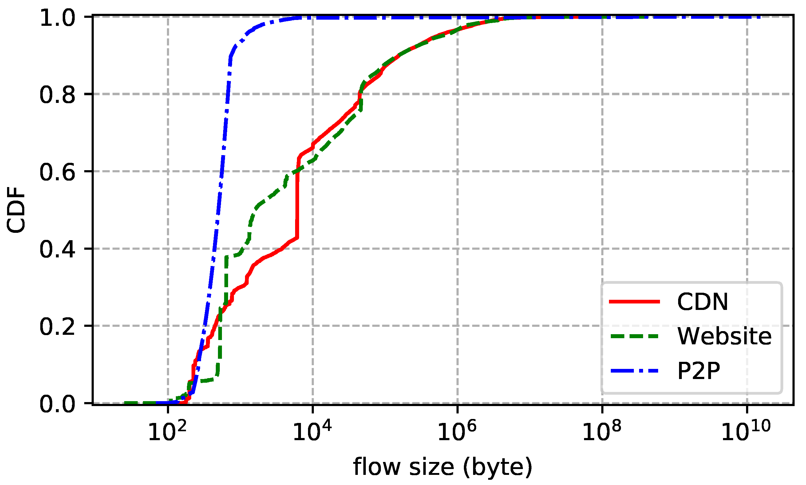
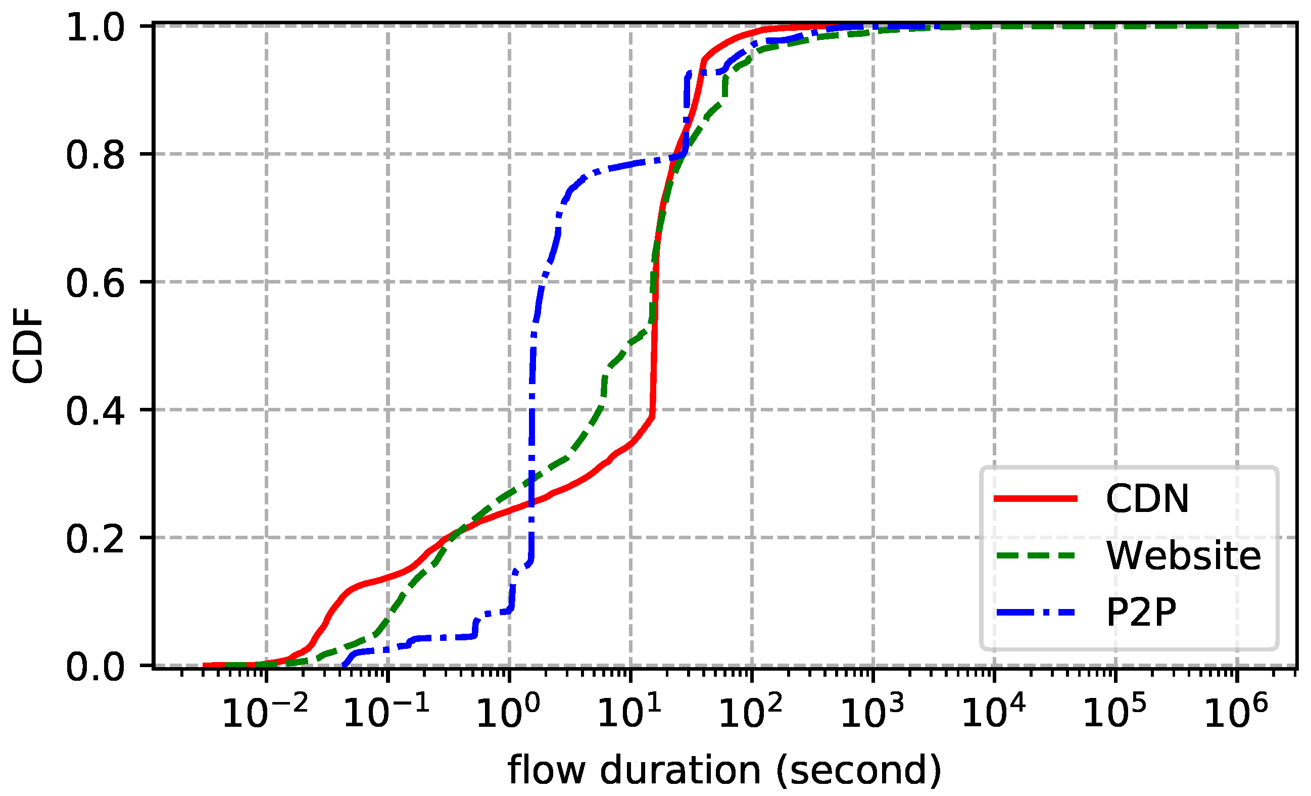
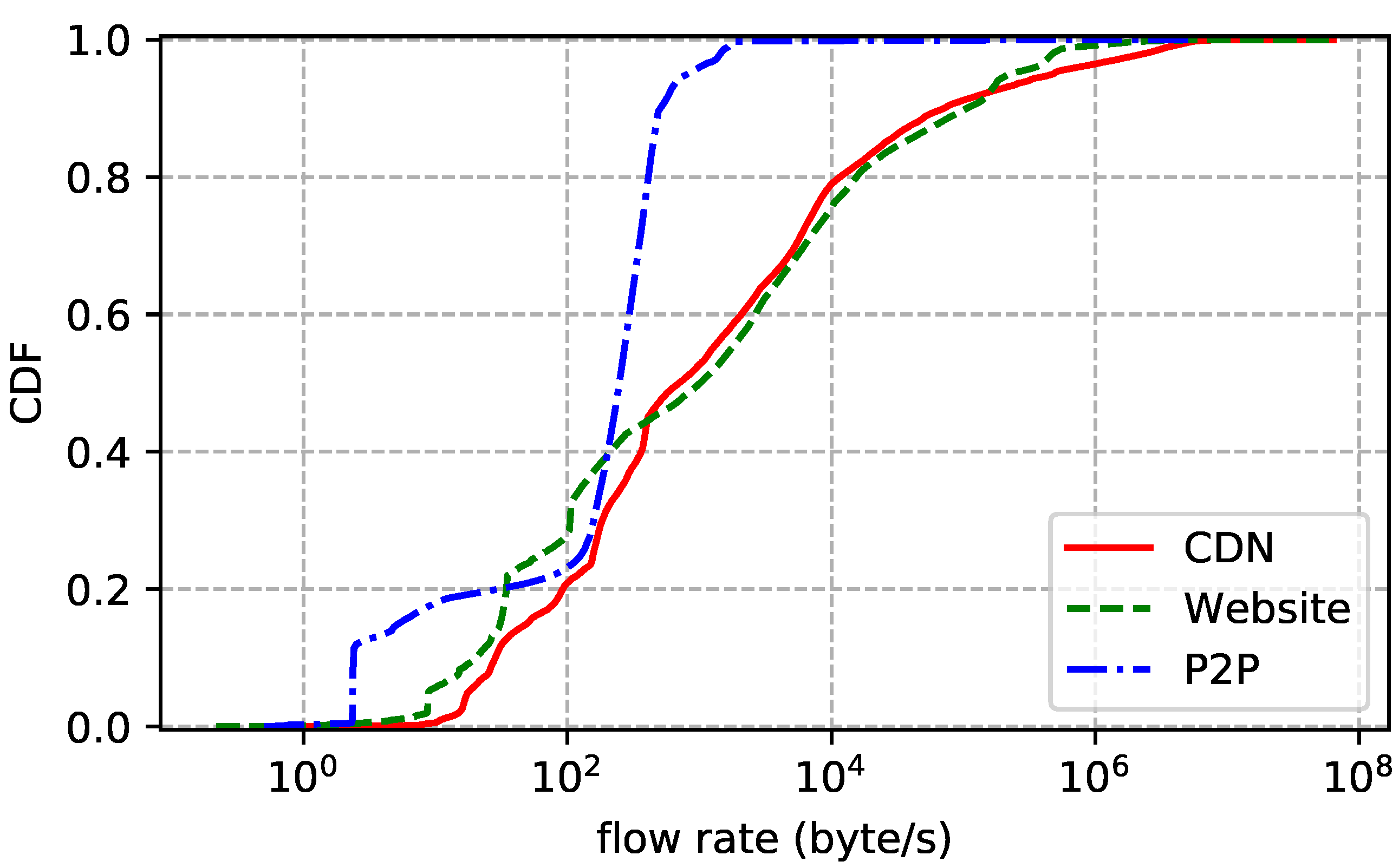
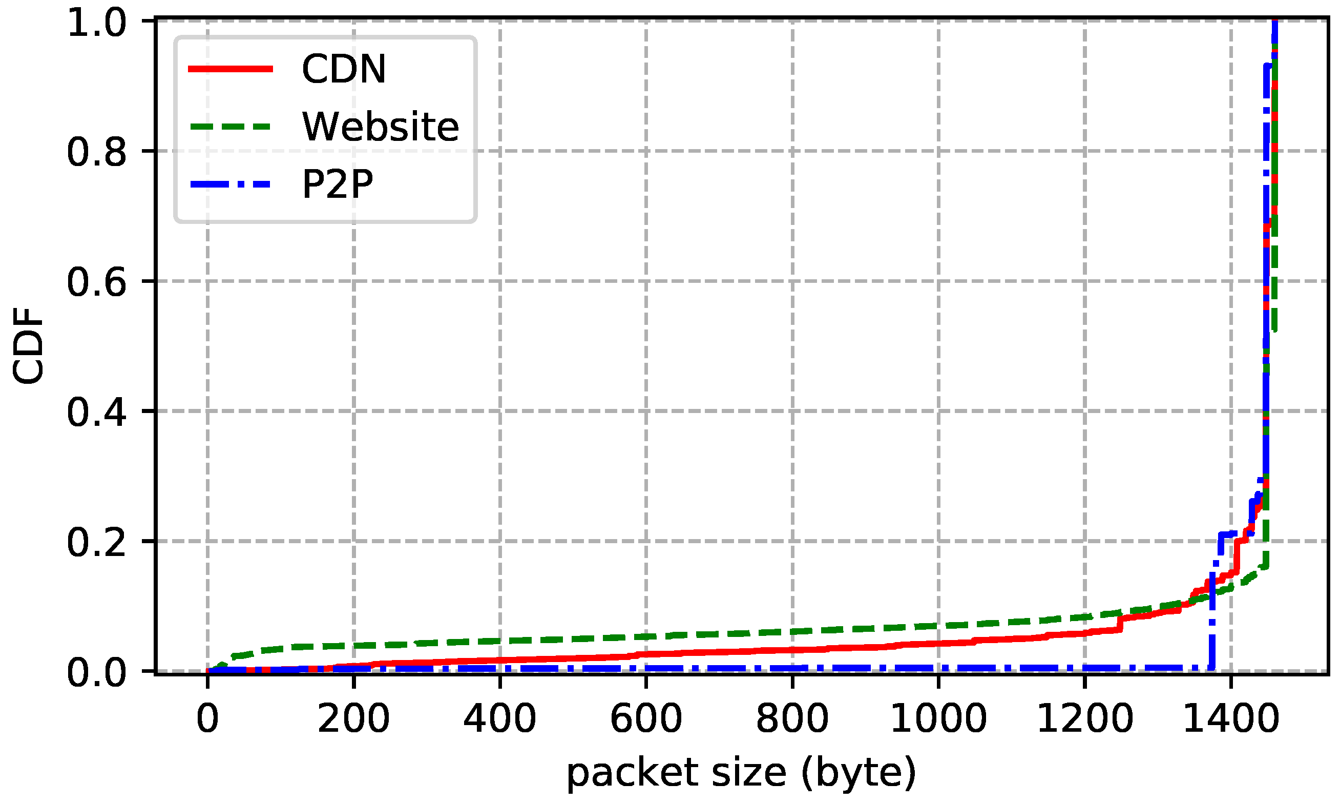
The statistics of the traces are summarized in Table 2. We also show the distributions of flow duration, size, and rate of each trace. Flow duration is the time between the first packet and the last one. Flow size is the number of bytes transmitted in the payload, including retransmissions. Flow rate is just size divided by duration. In addition, we report the packet size (header excluded) statistics to further understand the characteristics of the traces. Note that we only count packets with payload. The flow size distribution plotted by Figure 2 shows that more than 60% of the flows transmit less than 10 KB data and more than 95% of the flows transmit less than 1 MB data. In other words, most flows are small. Figure 3 reports similar statistics: more than 80% of the flows live shorter than 30 s and more than 94% of the flows live shorter than 100 s. Flow rate distribution shown in Figure 4 is also similar: more than 60% of the flows are slower than 30 KB/s and more than 95% of the flows are slower than 1 MB/s. Although most flows are slow, a few have rather high transmission rates. As for packet size distribution shown in Figure 5, it is not surprising that most data packets are MSS-sized.
5. Validation
In this section, we first evaluate EVA’s capacity on commodity machines, then validate our test environments, and finally evaluate whether EVA can pinpoint the performance problems at the right place and time.
5.1. Capacity
We used servers with Xeon 12-core, 2.4 GHz CPU, 64 GB memory and 10 Gbps Ethernet NIC. EVA captured packets from the NIC, grouped packets into flows, and stored these flows in a hash tables by a 4-tuple hash function. Note that packets were captured and analyzed in separate threads.
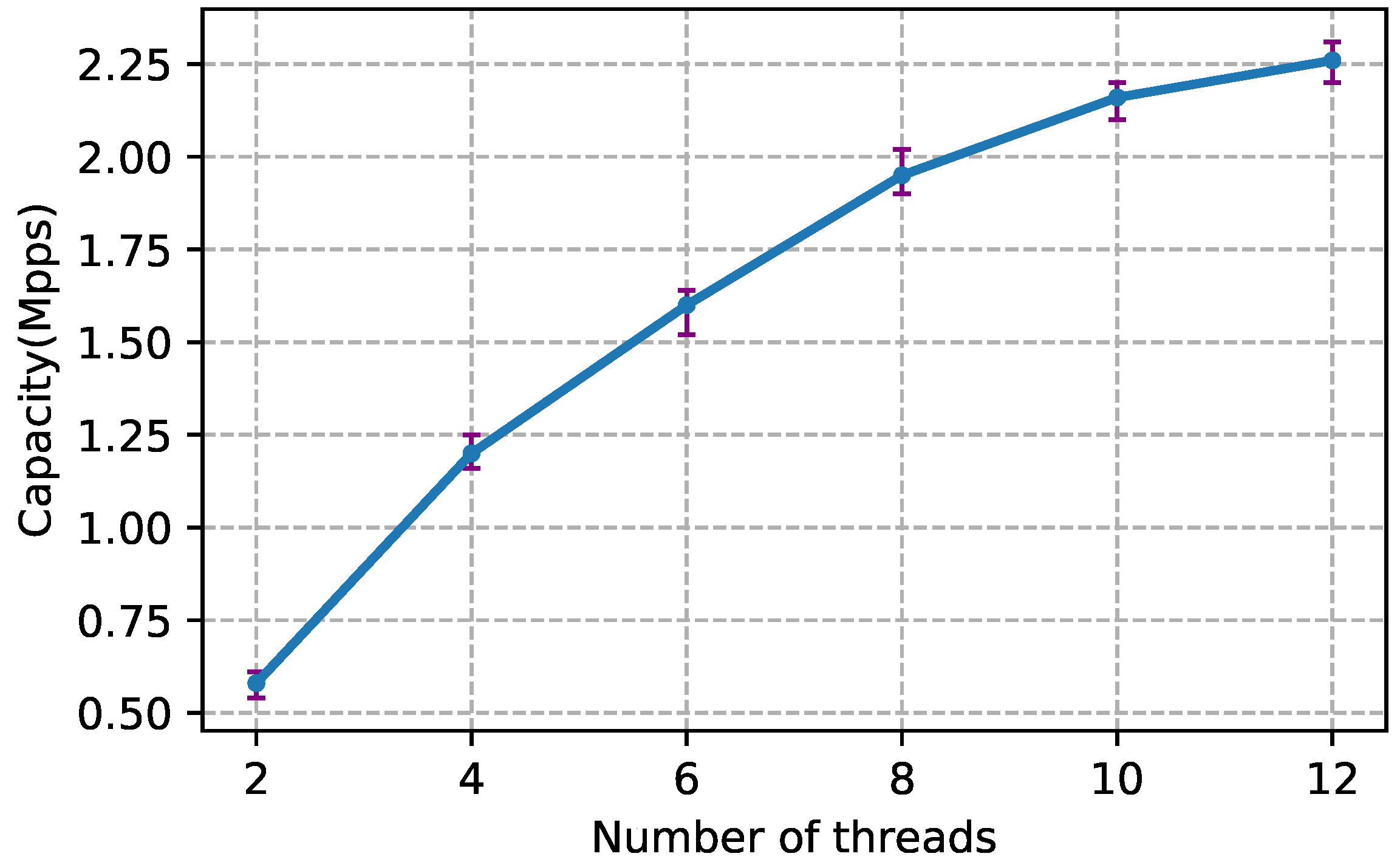
Since libpcap [36] does not support multithreaded capture, i.e., not scalable with the number of CPU cores, we used PF_RING [6], which is an extension of libpcap with ring buffers in the kernel to accommodate captured packets. More importantly, PF_RING supports multithreaded capture if the NIC enables RSS [37]. We evaluated EVA’s capturing and analysis part separately in single thread mode. The former achieved 700 Kpps without packet loss, and the latter achieved at least 600 Kpps. To evaluate EVA’s scalability, we tested its processing speed with different number of CPU cores. Specifically, we ran EVA with different number of threads, one thread per core, and then used Tcpreplay [38] to replay packet traces shown in Section 4 at increasing speed until packet loss occurred. Figure 6 shows that EVA scaled sublinearly with the number of CPU cores. As a result, with six capturing threads and six analysis threads, one server can process 2.26 Mpps with 12 cores.
While CPU limits the pps, memory limits the number of concurrent connections EVA can process. Note that they are independent metrics of EVA’s capacity. Since EVA buffers in flight packet headers for each flow, we must estimate the number of in flight packet per flow. On Linux, the default maximum send buffer is 4 MB and default MSS is 1460 (Figure 5 shows that most data packets are MSS-sized), thus about 4 MB/1460 B = 2873 packet headers per flow need to be stored in memory. For each flow, we need 408 B to store analysis status and 48 B per packet header. In total, we need 408 B + 2873 × 48 B = 135 KB per flow. Thus, each server can process around 64 GB/135 KB = 500 K concurrent connections. Table 2 shows that the number of maximum concurrent flows is no more than 1.5 K, which is far below EVA’s capacity.
5.2. Dummynet Validation
We validated EVA’s components on controlled testbed, which consisted of one machine running FreeBSD 11.1 and two machines running Ubuntu 18.04. The FreeBSD acted as router as well as bottleneck link, the other two machines send and received data across the bottleneck link. We used dummynet [39] in FreeBSD to emulate network path of particular BtlBw, RTprop and packet loss rate.
Before using the testbed, we verified the accuracy of dummynet with various configurations. We first set the bandwidth and delay by dummynet, then used iPerf [40] to measure the actual bandwidth. For each configuration, we measured 10 times and then averaged. Figure 7 reports the accuracy of dummynet bandwidth configuration. With the increase of bandwidth and delay, dummynet’s accuracy became lower. In other words, we cannot pick too high bandwidth and delay when testing EVA. We also measured the delay for each configuration and found that the error was always below 1 ms, which was acceptable.
5.3. Performance Limit Validation
We validated EVA’s analysis results by systematically generating TCP flows with predetermined limiting factors. We built environments of different limiting factors, generated TCP flow by simple server and client programs, captured packet traces on server NIC, analyzed them by EVA, and compared the results with our expectations. Unless otherwise noted, the bandwidth and delay were 40 Mbps and 30 ms, respectively. For each set of experiments, we set up Cubic and BBR on server to evaluate the effect of different congestion controls on EVA. In most cases, EVA correctly identified the performance problems of a flow. However, when carefully observing each flight within a flow, we found a few erroneous diagnoses, but still acceptable. In the following, we show a series of experiments as well as the validation results.
Slow start limited. In slow start limited tests, we set up a FTP server providing files ranged from 10 KiB to 1000 KiB, incremented by 10 KiB. For all connections, EVA successfully identified the first few flights as slow start limited. For Cubic server, the first fie flights (about 310 KiB) were deemed slow start limited. For BBR server, the first six flights (about 630 KiB) were deemed slow start limited. We carefully examined the time series diagrams of these traces and successfully verified the above results. The slow starting of BBR is one flight longer than that of Cubic, because the former takes a more aggressive slow start strategy.
Receive window limited. In these tests, we transferred a 10MB file with different configurations of client. We did two sets of experiments: fixing receive buffer size by Linux SO_RCVBUF socket option and fixing retrieve speed of the client application. In the first set of experiments, the receive buffer ranged from to ( KiB), incremented by . For both Cubic and BBR server, connections of receive buffer size smaller than were deemed receive window limited, and the rests were deemed bandwidth limited. We expected this critical point to be instead of . In fact, EVA already detected the right BtlBw since , however, diagnostic of receiver took precedence over network.
In the second set of experiments, client application retrieve speed varied from to , incremented by . We also increased the file size to 100 MiB to ensure the receive buffer being filled. EVA successfully identified all connections as receive window limited except the one. Since TCP dynamically adjusted the size of receive buffer, EVA also detected several bandwidth limited flights right after slow start.
Congestion limited. In congestion limited tests, we injected 10 Mbps UDP traffic into network for a period of time while transferring files. For all connections, EVA successfully identified all flights during the period as congestion limited. We also observed congestion control limited flights right after congestion limited flights, and Cubic had more such flights than BBR. This is because both BBR and Cubic probed the available bandwidth after network congestion, and BBR was faster.
Send buffer limited. In these tests, we transferred 10 MB files with different send buffer sizes of the server (use SO_SNDBUF socket option), which ranged from to , incremented by . Connections of send buffer size less than were successfully deemed send buffer limited. However, EVA also reported some application limited flights of these connections, especially when the buffer was small. We carefully inspected the packet traces and found less-MSS-sized packets in these flights, and these packets caused incorrect diagnoses of EVA.
Application limited. Similar to the previous tests, 10 MB files were transferred from server to client. The server randomly wrote 1 to 10 MSS bytes to network stack for randomly 1 to 100 ms, with TCP_NODELAY and tcp_autocorking options turned on or off. EVA identified all connections as application limited. However, for BBR server, when TCP_NODELAY is off and tcp_autocorking is on, EVA reported some congestion control limited flights, since the network stack tried to coalesce small writes as much as possible, decreasing the number of less-MSS-sized packets.
Congestion control limited. Congestion control limited was tested by transferring 10 MB files, with packet loss rate induced by dummynet, ranged from 1% to 10%, incremented by 1%. EVA reported totally different results of Cubic and BBR: Cubic connections were deemed congestion control limited, while BBR connections were deemed bandwidth limited. This is not hard to explain: Cubic interpreted loss as a signal of congestion, but BBR did not. There is a point to make about the experiments. For Cubic connections, EVA was unable to observe real BtlBw due to extremely low throughput. Nonetheless, EVA still correctly identified these connections as congestion control limited.
Bandwidth limited. To validate bandwidth limited, we transferred 10 MB files with on other competing flows in the network. Send and receive buffers were auto adjusted by network stack, and packet loss rate were set to zero by dummynet. EVA not only identified all connections as bandwidth limited, but also reported the right BtlBw and RTprop.
Bufferbloat limited. Bufferbloat limited was tested by transferring 100 MB files. The bottleneck buffer was set to 1 MB by dummynet, which was large enough to introduce high delay. Again, EVA reported totally different results of Cubic and BBR: Cubic connections were deemed bufferbloat limited, while BBR connections were not. To explain this, the principles of Cubic and BBR must be understood. Cubic is loss-based thus keeps the bottleneck buffer full, while BBR explicitly controls the queue size in bottleneck link.
More than one limiting factors. After validating the limiting factors one by one, we further evaluated EVA’s performance by simultaneously generating flows with different performance problems. Since network resources were shared, flows that monopolize the resources can greatly affect the transmission of the others. More specifically, if the network path is already saturated, host limited (application limited, receive window limited, etc.) flows may suffer network congestion or bufferbloat unexpectedly. To avoid this ambiguity, we only validated host limited flows. In particular, we set up four long-lived flows, each limited by application, send buffer, receive window and congestion control. At the same time, we repeatedly generated short-lived flows (transfer 100 KB files) to validate slow start limited. In other words, at any given time, there were five flows in the network.
The test lasted for one minute and 5708 flights were collected. Based on the diagnosis of each flight, Table 3 reports EVA’s accuracy for each host limiting factor. We can see that EVA achieved 0.80 in recall of slow start limited, which was lower than other limiting factors. We carefully inspected the slow start limited packet traces and found that the last flights did not satisfy the exponential relationship due to insufficient data.
6. Observations
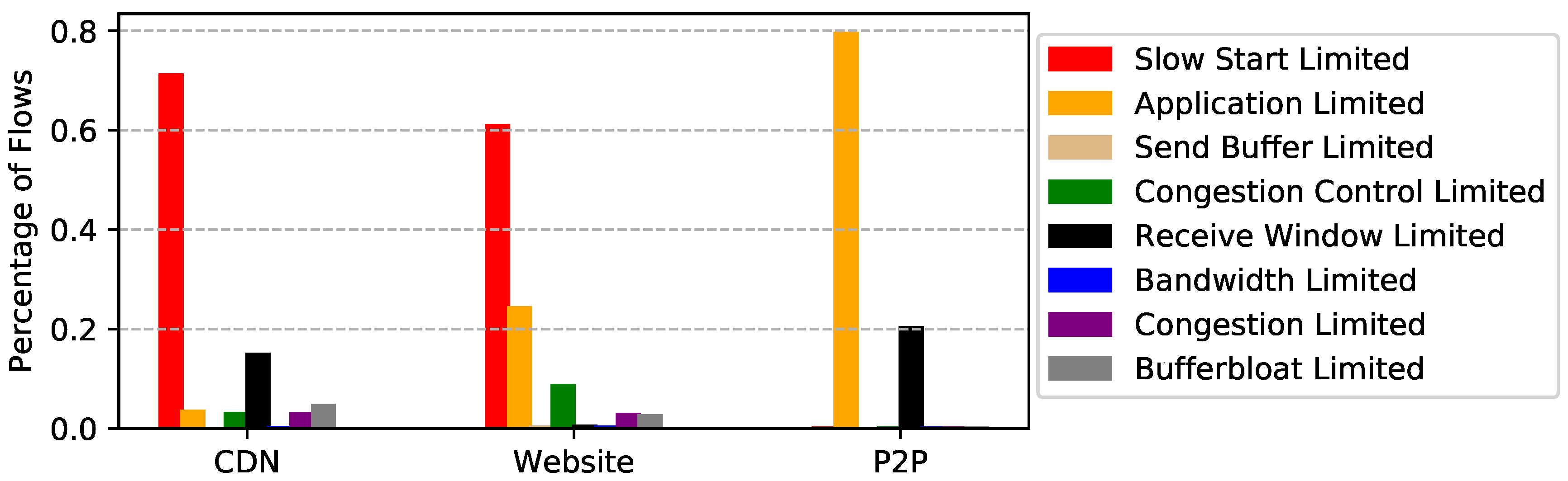
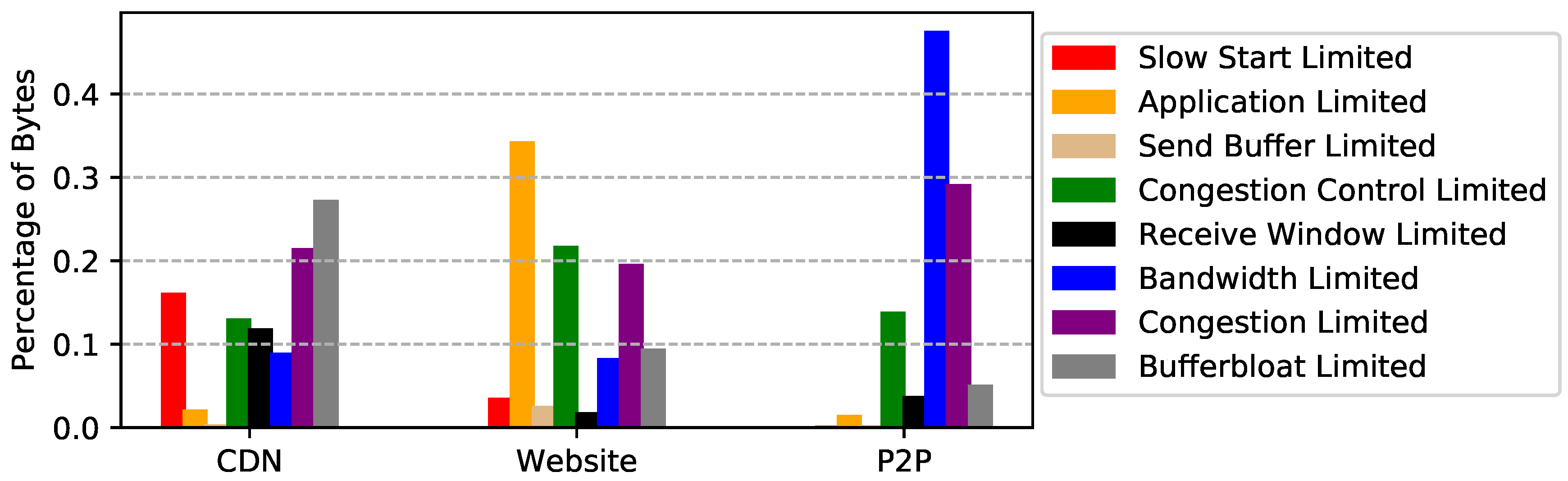
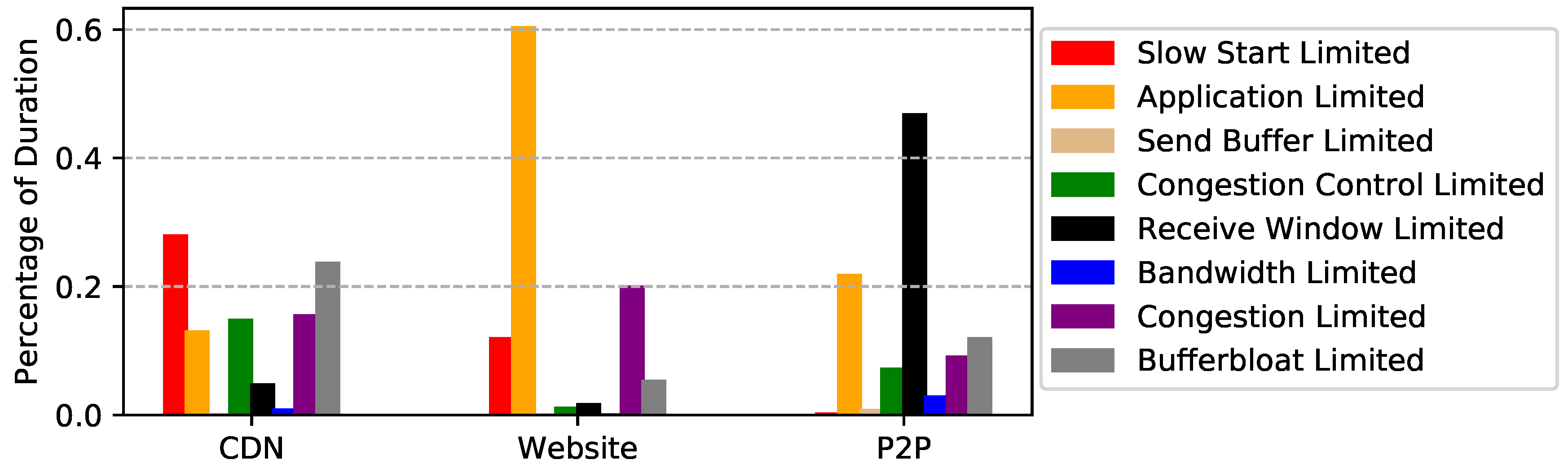
We apply EVA to the three packet traces and show the result in Figure 8, Figure 9 and Figure 10. Figure 8 shows the percentage of flows for each limiting factor. Remember that a flow may suffer several performance problems during its lifetime, especially long-lived TCP connections. For example, for a file transferring flow, it saturates the bottleneck link after slow start, and finally ends up with network congestion. For simplicity, we use the most frequent limiting factors among all the flights to represent the dominating bottleneck of a flow. Since it is easy to obtain the size and duration of each flight of each flow, we also show the percentages of bytes and duration for each limiting factor in Figure 9 and Figure 10. In the following, before explaining the results of each dataset and giving suggestions for improvement, we show the relationship between flow statistics and performance limitations.
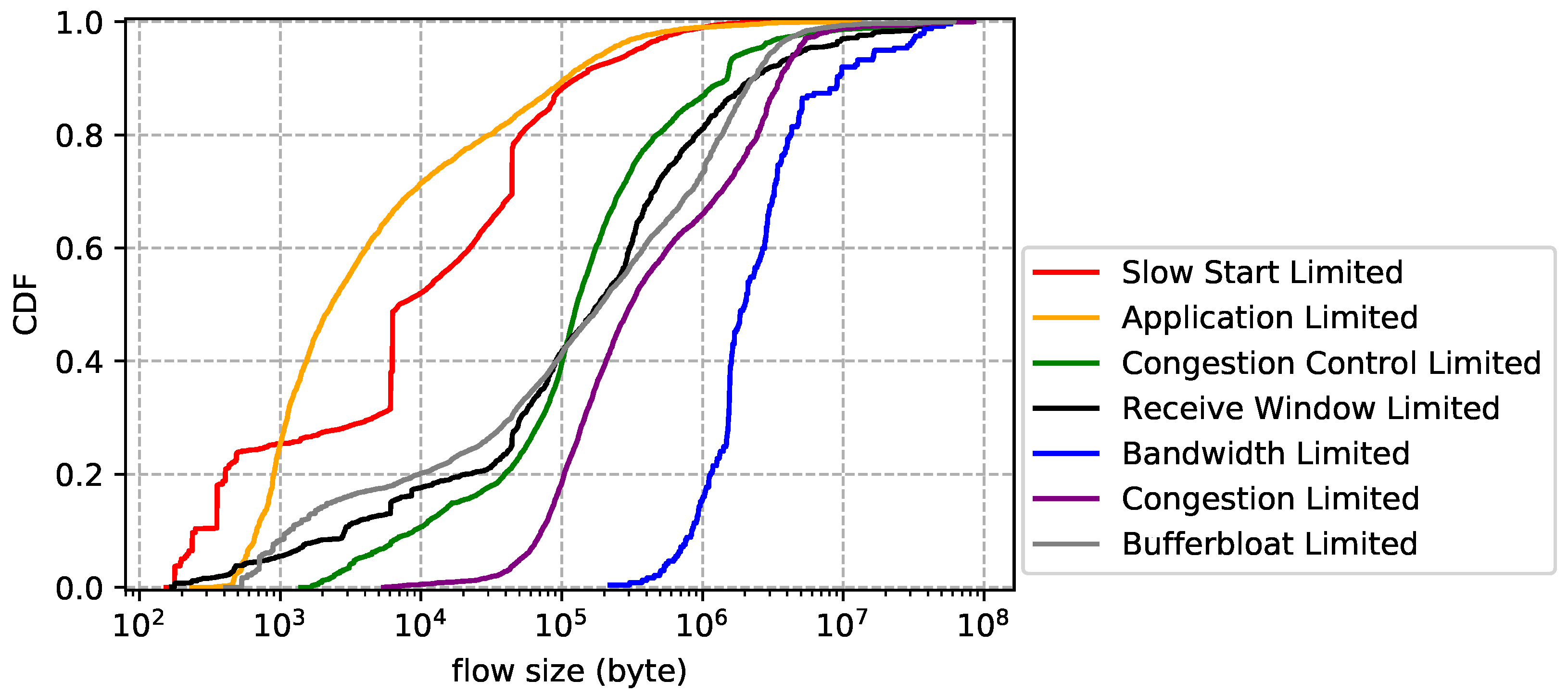
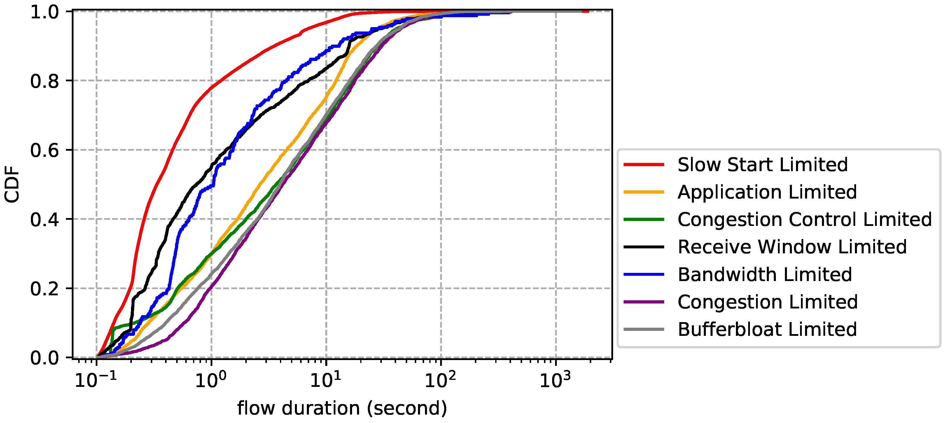
Flow statistics for each limiting factor. The flow size distribution is reported by Figure 11. Overall, bandwidth limited flows have the largest average size, followed by congestion limited, while application limited flows have the smallest average size, followed by slow start limited. The results are easy to understand: flows that transfer bulk data are more likely to cause network performance problems than others. The flow duration distribution is plotted by Figure 12, which shows that slow start limited flows have the shortest average lifetime and congestion limited flows have the longest average lifetime. We also notice that application limited flows are not necessarily short-lived and bandwidth limited flows are not necessarily long-lived. In other words, big size does not mean long lifetime and vice versa. Finally, we show the flow rate distribution in Figure 13. Unsurprisingly, bandwidth limited flows have the largest average rate and application limited flows have the smallest average rate.
CDN packet trace. As shown in Figure 8, more than 71% of the flows are slow start limited, i.e., they are short-lived flows. This is not surprising since most images the CDN server delivered were small. However, when turning our eye to the fraction of bytes for each limiting factor, we find that bufferbloat and congestion account for 48% of the traffic. More surprisingly, only 7% of the flows are identified as bufferbloat or congestion limited. Therefore, we suggest to first find the source of the network problem. If the problems are self-inflicted, better congestion controls can alleviate this. Otherwise, ISPs that provide better network environments should be considered.
Website packet trace. Similar to CDN packet trace, slow start limited accounts for 61% of the flows. We also notice that application limited accounts for 34% and 60% of the bytes and duration, respectively. This is mainly because many HTTP sessions are long-lived and interactive. In addition, Figure 9 shows that 22% of the bytes are congestion control limited, which implies the congestion control could have used network bandwidth more efficiently.
P2P packet trace. Interestingly, even though 79% of the flows are application limited, this limitation only accounts for 5% of the traffic. This means that most TCP connections are not used for file transfers. Unsurprisingly, bandwidth limited accounts for 47% of the traffic. In other words, P2P performance can be further improved if more bandwidth is available. It is worth noting that receive window limited accounts for 47% of the duration. This is probably not a performance problem since P2P users may deliberately limit download speed.
7. Conclusions
In this paper, we present EVA, a diagnostic tool that pinpoints network performance problems. It monitors packet streams near the server, estimates essential TCP metrics, and finds performance bottlenecks of each flow. Application developers and network operators can leverage the results to troubleshoot network problems. Experiments show that our solution is generic and accurate enough to work with various applications and congestion controls. Based on the results of applying EVA to several packet traces, we pinpoint the major performance limitations and give possible solutions.
We plan to improve the tool and expand the scope of application of the tool in the future work. In particular, we want to ensure the correctness of the analysis results when faced with middleboxes (traffic shaper, traffic policer, etc.) in the network path.
Author Contributions
Conceptualization, G.X. and Y.-C.C.; Methodology, G.-Q.P. and Y.-C.C.; Software, G.-Q.P.; Validation, G.-Q.P. and Y.-C.C.; Investigation, G.-Q.P.; Resources, G.X.; Data Curation, G.X. and G.-Q.P.; Writing—Original Draft Preparation, G.-Q.P.; Writing—Review and Editing, G.-Q.P., Y.-C.C. and G.X.; Supervision, Y.-C.C. and G.X.; and Project Administration, Y.-C.C. and G.X.
Funding
This work is supported by National Key R&D Program of China (2017YFC0803700), the Joint Key Project of the National Natural Science Foundation of China (Grant No. U1736207), NSFC (No. 61572324), Shanghai Talent Development Fund, and Shanghai Jiao Tong arts and science inter-project (No.15JCMY08).
Conflicts of Interest
The authors declare no conflict of interest.
References
- Gettys, J.; Nichols, K. Bufferbloat: Dark Buffers in the Internet. Commun. ACM 2012, 55, 57–65. [Google Scholar] [CrossRef]
- Nagle’s Algorithm. Available online: https://en.wikipedia.org/wiki/Nagle%27s_algorithm (accessed on 4 June 2018).
- Cardwell, N.; Cheng, Y.; Gunn, C.S.; Yeganeh, S.H.; Jacobson, V. BBR: Congestion-based Congestion Control. Commun. ACM 2017, 60, 58–66. [Google Scholar] [CrossRef]
- Arzani, B.; Ciraci, S.; Loo, B.T.; Schuster, A.; Outhred, G. Taking the Blame Game out of Data Centers Operations with NetPoirot. In Proceedings of the 2016 ACM SIGCOMM Conference, Florianopolis, Brazil, 22–26 August 2016; pp. 440–453. [Google Scholar]
- Ha, S.; Rhee, I.; Xu, L. CUBIC: A New TCP-friendly High-speed TCP Variant. SIGOPS Oper. Syst. Rev. 2008, 42, 64–74. [Google Scholar] [CrossRef]
- PF_RING: High-Speed Packet Capture, Filtering and Analysis. Available online: https://www.ntop.org/products/packet-capture/pfring (accessed on 4 June 2018).
- Zhang, Y.; Breslau, L.; Paxson, V.; Shenker, S. On the Characteristics and Origins of Internet Flow Rates. In Proceedings of the 2002 Conference on Applications, Technologies, Architectures, and Protocols for Computer Communications, Pittsburgh, PA, USA, 19–23 August 2002; pp. 309–322. [Google Scholar]
- Zhu, Y.; Kang, N.; Cao, J.; Greenberg, A.; Lu, G.; Mahajan, R.; Maltz, D.; Yuan, L.; Zhang, M.; Zhao, B.Y.; et al. Packet-Level Telemetry in Large Datacenter Networks. In Proceedings of the 2015 ACM Conference on Special Interest Group on Data Communication, London, UK, 17–21 August 2015; pp. 479–491. [Google Scholar]
- Benko, P.; Malicsko, G.; Veres, A. A large-scale, passive analysis of end-to-end TCP performance over GPRS. In Proceedings of the IEEE INFOCOM 2004, Hong Kong, China, 7–11 March 2004; Volume 3, pp. 1882–1892. [Google Scholar]
- Sundaresan, S.; Feamster, N.T.R. Measuring the Performance of User Traffic in Home Wireless Networks. Commun. ACM 2015, 8995, 57–65. [Google Scholar] [CrossRef]
- Botta, A.; Pescapé, A.; Ventre, G.; Biersack, E.; Rugel, S. Performance footprints of heavy-users in 3G networks via empirical measurement. In Proceedings of the 8th International Symposium on Modeling and Optimization in Mobile, Ad Hoc, and Wireless Networks, Avignon, France, 31 May–4 June 2010; pp. 330–335. [Google Scholar]
- Ricciato, F. Traffic monitoring and analysis for the optimization of a 3G network. IEEE Wirel. Commun. 2006, 13, 42–49. [Google Scholar] [CrossRef]
- Yu, M.; Greenberg, A.; Maltz, D.; Rexford, J.; Yuan, L.; Kandula, S.; Kim, C. Profiling Network Performance for Multi-tier Data Center Applications. In Proceedings of the 8th USENIX Conference on Networked Systems Design and Implementation, Boston, MA, USA, 30 May–1 April 2011; pp. 57–70. [Google Scholar]
- Cisco IOS NetFlow. Available online: https://www.cisco.com/c/en/us/products/ios-nx-os-software/ios-netflow/index.html (accessed on 4 June 2018).
- sFlow. Available online: https://en.wikipedia.org/wiki/SFlow (accessed on 4 June 2018).
- Cormode, G.; Korn, F.; Muthukrishnan, S.; Srivastava, D. Finding Hierarchical Heavy Hitters in Streaming Data. ACM Trans. Knowl. Discov. Data 2008, 1, 2:1–2:48. [Google Scholar] [CrossRef]
- Zhang, Y.; Singh, S.; Sen, S.; Duffield, N.; Lund, C. Online Identification of Hierarchical Heavy Hitters: Algorithms, Evaluation, and Applications. In Proceedings of the 4th ACM SIGCOMM Conference on Internet Measurement, Taormina, Sicily, Italy, 25–27 October 2004; pp. 101–114. [Google Scholar]
- Estan, C.; Varghese, G. New Directions in Traffic Measurement and Accounting. In Proceedings of the 1st ACM SIGCOMM Workshop on Internet Measurement, Pittsburgh, PA, USA, 19–23 August 2001; pp. 75–80. [Google Scholar]
- Zhao, Q.; Xu, J.; Liu, Z. Design of a Novel Statistics Counter Architecture with Optimal Space and Time Efficiency. SIGMETRICS Perform. Eval. Rev. 2006, 34, 323–334. [Google Scholar] [CrossRef]
- Narayana, S.; Tahmasbi, M.; Rexford, J.; Walker, D. Compiling Path Queries. In Proceedings of the 13th USENIX Symposium on Networked Systems Design and Implementation (NSDI 16), Santa Clara, CA, USA, 16–18 March 2016; pp. 207–222. [Google Scholar]
- Foster, N.; Harrison, R.; Freedman, M.J.; Monsanto, C.; Rexford, J.; Story, A.; Walker, D. Frenetic: A Network Programming Language. SIGPLAN Not. 2011, 46, 279–291. [Google Scholar] [CrossRef]
- Narayana, S.; Sivaraman, A.; Nathan, V.; Goyal, P.; Arun, V.; Alizadeh, M.; Jeyakumar, V.; Kim, C. Language-Directed Hardware Design for Network Performance Monitoring. In Proceedings of the Conference of the ACM Special Interest Group on Data Communication, Los Angeles, CA, USA, 21–25 August 2017; pp. 85–98. [Google Scholar]
- Tammana, P.; Agarwal, R.; Lee, M. Distributed Network Monitoring and Debugging with SwitchPointer. In Proceedings of the 15th USENIX Symposium on Networked Systems Design and Implementation (NSDI 18), Renton, WA, USA, 9–11 April 2018; pp. 453–456. [Google Scholar]
- Li, W.; Wu, D.; Chang, R.K.; Mok, R.K. Demystifying and Puncturing the Inflated Delay in Smartphone-based WiFi Network Measurement. In Proceedings of the 12th International on Conference on Emerging Networking EXperiments and Technologies, Irvine, CA, USA, 12–15 December 2016; pp. 497–504. [Google Scholar]
- Huang, J.; Qian, F.; Gerber, A.; Mao, Z.M.; Sen, S.; Spatscheck, O. A Close Examination of Performance and Power Characteristics of 4G LTE Networks. In Proceedings of the 10th International Conference on Mobile Systems, Applications, and Services, Ambleside, UK, 25–29 June 2012; pp. 225–238. [Google Scholar]
- Huang, J.; Xu, Q.; Tiwana, B.; Mao, Z.M.; Zhang, M.; Bahl, P. Anatomizing Application Performance Differences on Smartphones. In Proceedings of the 8th International Conference on Mobile Systems, Applications, and Services, San Francisco, CA, USA, 15–18 June 2010; pp. 165–178. [Google Scholar]
- Deng, S.; Netravali, R.; Sivaraman, A.; Balakrishnan, H. WiFi, LTE, or Both?: Measuring Multi-Homed Wireless Internet Performance. In Proceedings of the 2014 Conference on Internet Measurement Conference, Vancouver, BC, Canada, 5–7 November 2014; pp. 181–194. [Google Scholar]
- Nguyen, B.; Banerjee, A.; Gopalakrishnan, V.; Kasera, S.; Lee, S.; Shaikh, A.; Van der Merwe, J. Towards Understanding TCP Performance on LTE/EPC Mobile Networks. In Proceedings of the 4th Workshop on All Things Cellular: Operations, Applications, & Challenges, Chicago, IL, USA, 22 August 2014; pp. 41–46. [Google Scholar]
- Karrer, R.P.; Matyasovszki, I.; Botta, A.; Pescape, A. MagNets-experiences from deploying a joint research-operational next-generation wireless access network testbed. In Proceedings of the 2007 3rd International Conference on Testbeds and Research Infrastructure for the Development of Networks and Communities, Lake Buena Vista, FL, USA, 21–23 May 2007; pp. 1–10. [Google Scholar]
- Karrer, R.P.; Matyasovszki, I.; Botta, A.; Pescapé, A. Experimental Evaluation and Characterization of the Magnets Wireless Backbone. In Proceedings of the 1st International Workshop on Wireless Network Testbeds, Experimental Evaluation & Characterization, Los Angeles, CA, USA, 29 September 2006; pp. 26–33. [Google Scholar]
- Paxson, V.; Allman, M. Computing TCP’s Retransmission Timer. RFC 2988, RFC Editor. 2000. Available online: https://tools.ietf.org/html/rfc2988 (accessed on 4 June 2018).
- UCloud: Leading Neutral Cloud Computing Service Provider of China. Available online: https://www.ucloud.cn/ (accessed on 4 June 2018).
- High Performance Load Balancer, Web Server, & Reverse Proxy. Available online: https://www.nginx.com/ (accessed on 4 July 2018).
- A Fast, Easy, and Free BitTorrent Client. Available online: https://transmissionbt.com/ (accessed on 4 July 2018).
- TCP Segmentation Offload. Available online: https://en.wikipedia.org/wiki/Large_send_offload (accessed on 4 June 2018).
- TCPDUMP/LIBPCAP Public Repository. Available online: https://http://www.tcpdump.org/ (accessed on 4 June 2018).
- Receive Side Scaling on Intel Network Adapters. Available online: https://www.intel.com/content/www/us/en/support/articles/000006703/network-and-i-o/ethernet-products.html (accessed on 4 June 2018).
- Tcpreplay: Pcap Editing and Replaying Utilities. Available online: https://tcpreplay.appneta.com/ (accessed on 4 June 2018).
- Carbone, M.; Rizzo, L. Dummynet Revisited. SIGCOMM Comput. Commun. Rev. 2010, 40, 12–20. [Google Scholar] [CrossRef]
- iPerf: The TCP, UDP and SCTP Network Bandwidth Measurement Tool. Available online: https://iperf.fr/ (accessed on 4 June 2018).
Figure 1.
Group packets into flights.

Figure 2.
Flow size distribution of each dataset.

Figure 3.
Flow duration distribution of each dataset.

Figure 4.
Flow rate distribution of each dataset.

Figure 5.
Packet size (payload) distribution of each dataset.

Figure 6.
EVA’s scalability with the number of threads.

Figure 7.
Dummynet bandwidth comparing to iPerf measurement.

Figure 8.
Percentage of flows for each limiting factor.

Figure 9.
Percentage of bytes for each limiting factor.

Figure 10.
Percentage of duration for each limiting factor.

Figure 11.
Flow size distribution for each limiting factor (CDN trace).

Figure 12.
Flow duration distribution for each limiting factor (CDN trace).

Figure 13.
Flow rate distribution for each limiting factor (CDN trace).


Table 1.
Summary of EVA’s method to identify performance bottlenecks.
| Performance Bottleneck | Method |
|---|---|
| Slow start limited | Consecutive flight size fits the exponential relationship |
| Receive window limited | Minimum receive window size |
| Congestion limited | Packet retransmissions are seen and at least one RTT sample |
| Send buffer limited | Flight size and remains unchanged for at least three flights |
| Application limited | Flight size and at least one less-MSS-sized packet is seen |
| Congestion control limited | Flight size |
| Bandwidth limited | More than half of the delivery rate samples in the flight are large than |
| Bufferbloat limited | All the RTT samples are larger than |
Table 2.
Characteristics of three packet traces.
| Trace | Date | Size | Length | #Packets | #Flows | #Max Concurrent Flows |
|---|---|---|---|---|---|---|
| CDN | 1 March 2018 | 30 GB | 20 min | 32 M | 160 K | 1382 |
| Website | 2 January 2018 | 100 GB | 3 days | 98 M | 550 K | 459 |
| P2P | 10 January 2018 | 400 GB | 5 days | 431 M | 1 M | 59 |
Table 3.
EVA’s performance for different limiting factors.
| Limiting Factor | Precision | Recall | F1 Score |
|---|---|---|---|
| Slow start limited | 0.95 | 0.80 | 0.86 |
| Application limited | 0.98 | 0.99 | 0.98 |
| Send buffer limited | 0.91 | 0.98 | 0.94 |
| Receive window limited | 1.00 | 0.99 | 0.99 |
| Congestion control limited | 0.94 | 0.90 | 0.91 |
© 2018 by the authors. Licensee MDPI, Basel, Switzerland. This article is an open access article distributed under the terms and conditions of the Creative Commons Attribution (CC BY) license (http://creativecommons.org/licenses/by/4.0/).
Share and Cite
MDPI and ACS Style
Peng, G.-Q.; Xue, G.; Chen, Y.-C. Network Measurement and Performance Analysis at Server Side. Future Internet 2018, 10, 67. https://doi.org/10.3390/fi10070067
AMA Style
Peng G-Q, Xue G, Chen Y-C. Network Measurement and Performance Analysis at Server Side. Future Internet. 2018; 10(7):67. https://doi.org/10.3390/fi10070067
Chicago/Turabian StylePeng, Guang-Qian, Guangtao Xue, and Yi-Chao Chen. 2018. "Network Measurement and Performance Analysis at Server Side" Future Internet 10, no. 7: 67. https://doi.org/10.3390/fi10070067
Note that from the first issue of 2016, this journal uses article numbers instead of page numbers. See further details here.