1. Introduction: Challenges of Geovisual Analysis on Climatic Data
In recent years, scientists from different communities, such as climatology, sociology and statistics, have been collaborating towards a better understanding of atmospheric-oceanic-glacial conditions [
1,
2], long-term climate variations [
3,
4], and interactions between climate changes and human society [
5,
6]. Plenty of climate models have been developed as the results of these joint efforts and massive amounts of spatiotemporal data have been generated by running these models [
7]. Various analyses using climate data are incorporated with IPCC assessment reports [
8]. Moreover, as the climate change issue has become more salient and a growing number of open resources for climate study emerged, the public began to engage in climate research in different ways. For example, via the
climateprediction.net initiative, some people are contributing personal computing resources to run climate models [
9,
10].
Data produced by climate models are simulated values of climate conditions over space and time. In general, these data have the following characteristics:
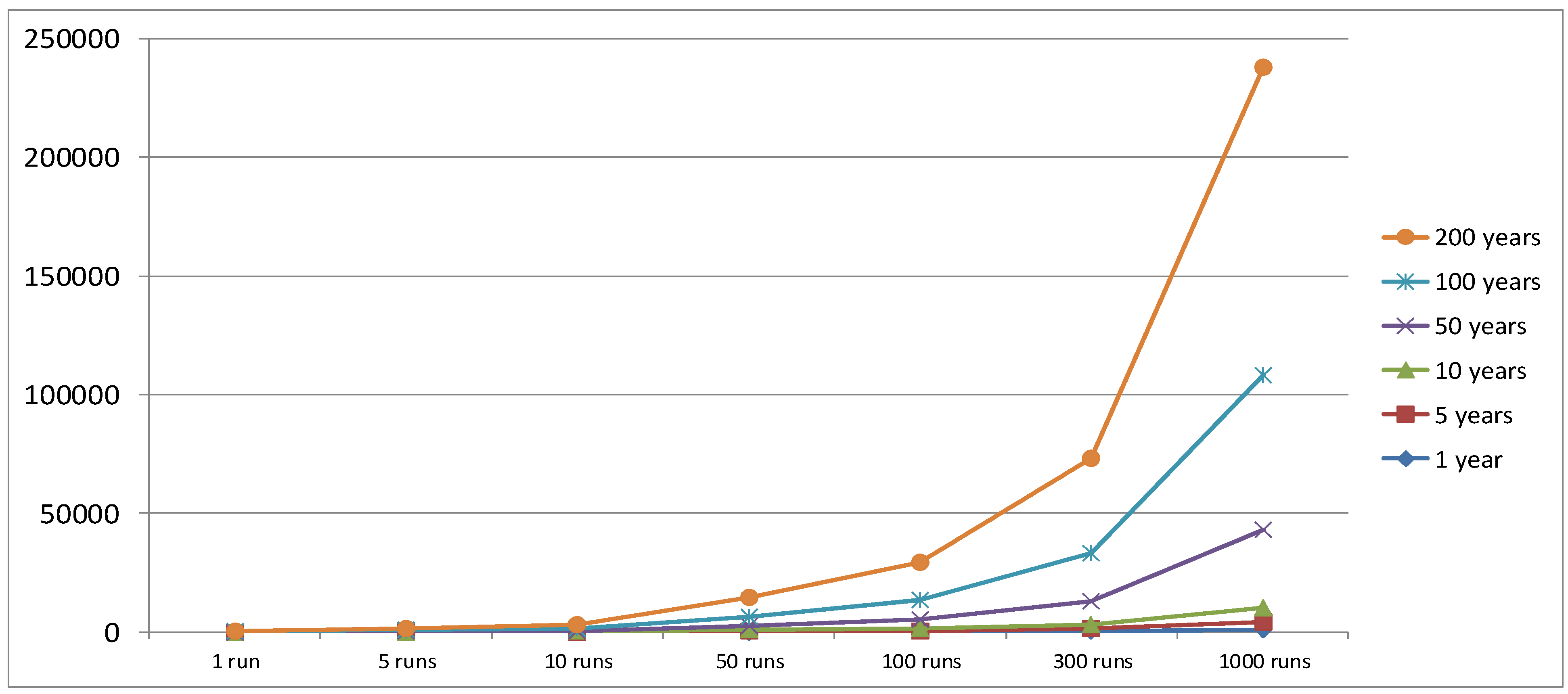
Due to the characteristics of the complex climate data, petabytes of spatiotemporal data are produced from running climate models (
Figure 1). Taking NASA Goddard Institute for Space Studies (GISS) ModelE as an example, outputs of ten-year monthly simulations from 300 model runs (one ensemble from thousands of ensembles) would yield 2.5 terabytes of data. Such large volumes of data are usually stored in distributed storage media. Geographically dispersed scientists and the public often access the data over the Internet. It is more convenient for data users to perform data visualization and analysis in a web-based environment. Visualizing and analyzing large spatiotemporal data in a web-based environment becomes a big challenge for climate researchers.
Figure 1.
ModelE data volume.
Figure 1.
ModelE data volume.
Traditional numerical and statistical methods have been frequently employed to analyze spatiotemporal climate data. The analysis results are usually represented as numerical data. However, humans have a relatively weak vision and cognition capability on identifying underlying principles from the overwhelming amounts of spatiotemporal information presented as textual and numerical data [
15]. Therefore, traditional approaches are not sufficient to visualize and analyze spatiotemporal data. In this case, approaches that represent information in visual products such as images are required to help researchers comprehend the information [
16]. In the context of geospatial sciences, geovisualization (e.g., maps) has been proved to be an efficient method for prompt understanding of complex geospatial data [
17]. Geovisual analytics integrates spatial analytical methods with geovisualization and is more powerful to reveal hidden patterns within geospatial data [
15]. Considering this capability, geovisual analytics is a potential solution for analyzing climate data.
However, several problems emerge when geovisual analytical tools are customized to support practical climate research: (1) Large spatiotemporal datasets require efficient strategies for data management and substantial computing resources; (2) The gap between existing statistical methods for climate studies and available geovisual representation solutions should be filled; (3) Interoperability amongst multiple statistical analyses on the climate data is needed; and (4) Interactive geovisual analytics over the Internet to facilitate collaborative climate research are immature. Solving these problems is both scientific and technical challenging. In this paper, we report the development of a web-based geovisual analytical system to conduct the spatiotemporal intensive and labor-intensive analytical processing of climate data. With the web-based system, users can visualize and analyze climate data interactively through a web interface. To demonstrate the usages of the system in real applications, we customize the system to facilitate the analysis of data produced by GISS ModelE [
11].
2. Related Work
A few geovisual analytical tools dealing with climate data have been developed. In the past, climate data were processed and analyzed in standalone computing resources [
18] using scientific packages, such as “NumPy” [
19] and “PyClimate” [
20]. Besides the well-developed packages, scientists might also develop their specialized statistical analysis scripts such as anomaly trend analysis using R to achieve particular research purposes [
21]. Although the analytical packages have plenty of professional analysis functions, they do have several limitations: (1) Packages written in various languages such as R, Python, FORTRAN and C are not interoperable. Researchers have to spend considerable amount of time on translating packages; (2) Except for some well-developed packages (e.g., NumPy), analytical tools designed by particular scientists are not shared with others. This circumstance leads to repeated developments of similar analytical functions, which is time consuming. The accuracy of analytical functions produced by developers without good scientific training is not guaranteed [
22]; (3) Generic functions on data management and data processing like regridding, data format conversion, and metadata editing are missing. Data preprocessing is necessary before employing the packages for analysis. In addition, since software packages are launched on standalone computers, data analysts have to spend time on transferring data to a local machine where tool is installed when dealing with large distributed data. This process requires large data storage, large network bandwidth and enough computing resources on personal computing facilities.
In order to overcome the deficiencies of standalone applications, analytical packages that integrate functions for data processing, visualization and analysis were developed. For example, the Climate Data Analysis Tool (CDAT) [
23] is a set of utilities designed for climate research on large volume data sets. CDAT provides capabilities including: (1) management and remote access of data sets; (2) data preprocessing such as regridding and format conversion; (3) functions for advanced statistical and numerical analysis; and (4) multiple 2D or 3D data visualization, for example, ViSUS system [
24]. As a component of geovisual analytical tools, a graphical interface is provided to users to interactively invoke CDAT functions. Without the interface, users have to conduct analysis by typing Python commands. However, despite strong data processing and analytical capabilities, CDAT did not address the limitations discussed above related to launching packages on standalone computers. Also, CDAT requires users to install multiple packages on their machines. In addition, these highly professional tools require users to have knowledge of climatology and some programming skills. The similar deficiencies have also been identified in Ultra Volume-CDAT (UV-CDAT).
With the popularity of Web 2.0 [
25], online systems should be used for geovisual analytics for climate data. A web-based visualization platform developed by Sun [
26] offers management and 3D rendering of distributed climate data from different vendors. Simple map operations and statistical plots like line plot of time series are supported through web browsers. Open Statistics eXplorer-platform [
27], another web-based geovisual analytical system, provides a good interactive graphical data representation [
15]. The system enables dynamic querying over graphs and linkages between different maps and statistical plots. Users can customize map symbolization through interface as well. Such web-based systems partially address the deficiencies of using local machines to process climate data by integrating all data processes in a single point. Data analysts no longer need to transfer data and develop geovisual analytical functions. However, none of the two systems contains sufficient data processing and advanced analysis functions for climate research, such as calculating Taylor diagram for detecting the quality of simulation [
28]. The capabilities of managing large volume datasets and representing complex spatiotemporal data are inadequate.
In summary, there is plenty of room to improve the existing geovisual analytical tools for climate studies. On one hand, standalone systems require adequate computing resources on local machines for large data sets, professionally trained scientists to conduct complex analysis, and much time on data pre-processing and function redevelopment. On the other hand, web-based systems do not included sufficient analytical functions for spatiotemporal analysis on climate data. We developed a web-based geovisual analytical prototype that can overcome some limitations of the existing systems.
3. System Design
Generally, a web-based geovisual analytical system includes front-end clients, application services and back-end data repositories [
17]. To implement each component, the first step is to analyze the functional requirements of geovisual analytical for climate data. The typical information that statistical analysis should detect from climate data are mean values, correlation between variables, stationarity over time series, quality of forecasting, and spatiotemporal patterns [
29]. Most analyses only use model simulation data, but the validation of simulation also requires observation data in addition to model simulation data. Except mean calculation, all the other analyses are performed based on the mean value over a certain time period. Therefore, certain frequently used mean values should be pre-calculated and stored as initial statistics. Data analysis can be divided into simple and high-level types. Simple analyses like intuitively observing spatiotemporal patterns or difference between simulation and observation can be implemented directly through data comparisons. High-level analyses such as detecting correlation and anomalies need to be sent to the server side for complex processing. Graphic representation of results is required for final results presentation.
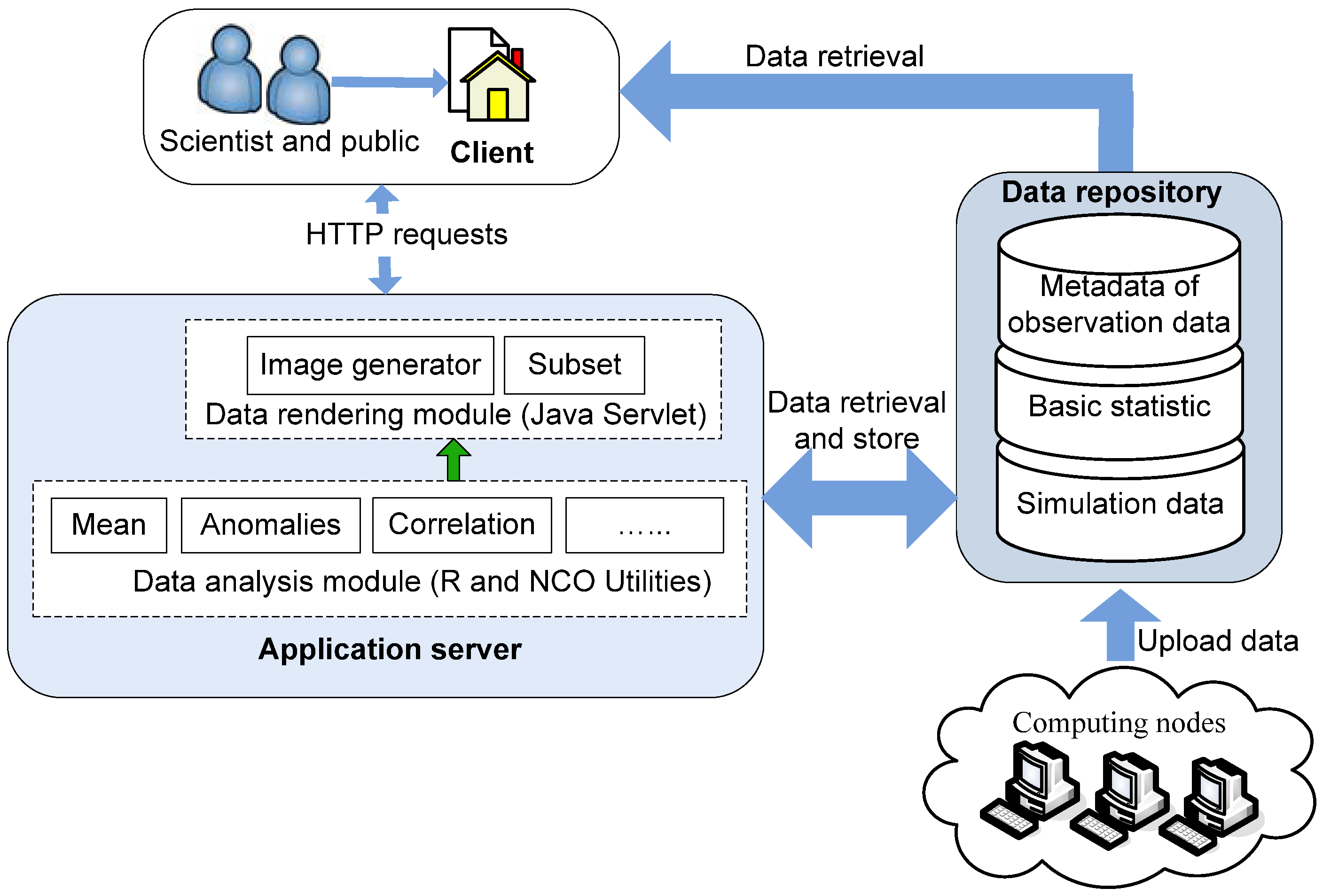
Therefore, our system is designed to include three functional components (
Figure 2): (1) the data repository to store data or metadata from simulation, observation and initial statistics; (2) the application server to provide data processing and high-level analytical functions; and (3) the web-based client to perform simple analysis and display visualization results with interactive tools.
Figure 2.
System architecture.
Figure 2.
System architecture.
3.1. Data Repository
The data repository maintains data sources, metadata of data sources and statistical results generated by initial data processing.
3.1.1. Simulation and Observation Data
Data sources include both model simulation data and metadata of observation data. Climate model simulation data are usually stored in the formats of HDF, HDF-EOS and NetCDF [
26]. We use NetCDF as an example in this paper. When a simulation is finished on a distributed computing node, the outputs are uploaded into the repository server for centralized management. The metadata entry recording basic information of outputs such as spatiotemporal coverage, variables, and computing node is inserted into the database. We do not host observation data provided by the other vendors in the repository but only manage the metadata of observation in the database. Data analysts need to acquire observation data from original providers when observation data are required by analysis. The system will assist in automatic data preprocessing.
3.1.2. Data Preparation and Initial Statistics
Climate analysis often uses quarterly or monthly average data over a long time period, and statistics like the annual mean are often required, though different applications may require higher-order statistics based on high-frequency output too. Pre-processing of model simulation data is often required before advanced analyses and visualizations [
30].
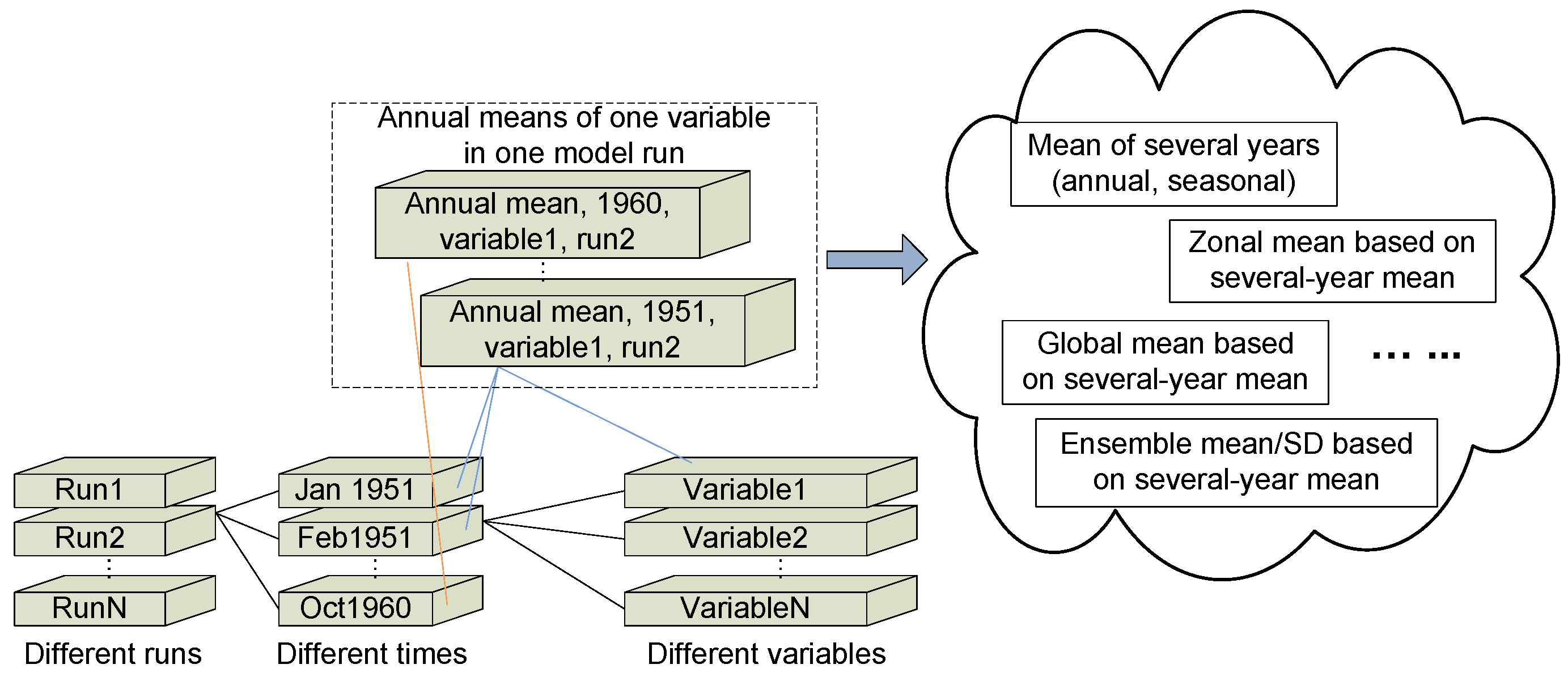
How data pre-processing reduces the time spent on data analysis should be investigated based on data structures and particular application demand for data analysis. As shown in
Figure 3, general climate models include multiple model runs, multiple monthly or daily based outputs in each run, and multiple variables in each data unit. According to previous studies [
24,
31,
32], annual mean is one of the most frequently used values for further analysis, thus it should be pre-calculated. Other data calculations such as multiple year annual mean, zonal mean, global mean, ensemble mean and ensemble standard deviation can be extracted on-the-fly when needed from the basic annual mean. Similar strategies are also possible with other kinds of averaging (such as daily, monthly, or seasonal climatologies). We demonstrate the efficiency of this strategy in
Section 4.3.
Figure 3.
Model simulation data structure and data preparation.
Figure 3.
Model simulation data structure and data preparation.
In addition, images that are easy to be transferred through Internet are generated and stored in the data repository for visualization purposes. Each NetCDF file is associated with image files. Requests from the client side for data visualization only retrieve images.
MySQL [
33] is selected to manage metadata in the system because of its wide usage, free availability and ability to store and retrieve large datasets.
3.2. Application Server
The application server provides multiple data processing and analytical functions to support requests from clients in real-time for advanced analyses and visualization of climate data. These functions can be categorized into two modules: data analysis module and data rendering module.
3.2.1. Data Analysis Module
As mentioned in the literature review, several analysis packages for statistical analysis in climate research have been developed. This system intends to integrate the commonly used analytical functions in the data analysis module.
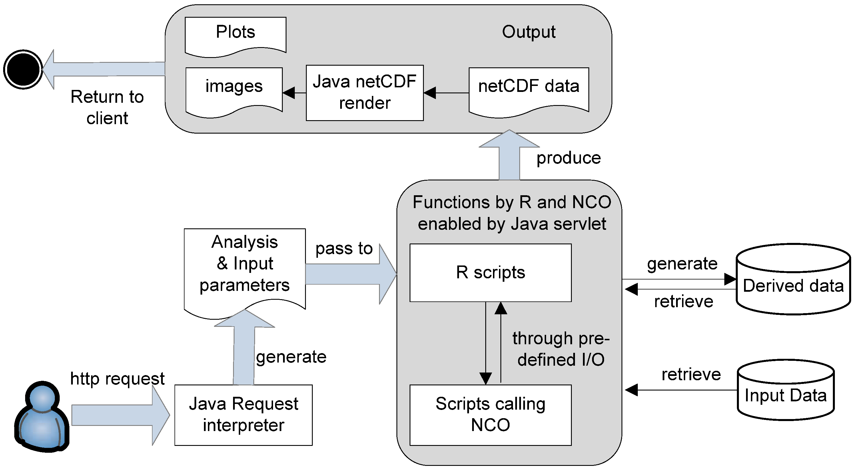
The workflow of executing analysis requests is shown in
Figure 4. Users define their analysis requirements such as variable, spatiotemporal coverage, analysis type and representation form. The requests are then sent to the application server through HTTP. Input parameters in HTTP are interpreted and the corresponding analytical functions are invoked on the server side. When executing the analysis, selected input data (e.g., 1-year annual means) are retrieved from the original database and processed to satisfy the data input requirement of the analysis functions. The analysis process may generate some temporary data (e.g., 10-year annual mean) which are deleted after the completion of the analysis. The final output may be new NetCDF data or graphs of statistical plots. The NetCDF data which cannot be rendered by clients directly should be converted into images. The response is returned to users as an XML stream which includes the information about analysis output such as path, title and legend.
Figure 4.
Workflow of the application server.
Figure 4.
Workflow of the application server.
The entire workflow is enabled by HTTP requests, Java servlets and XML. NetCDF Operator (NCO) software [
34] is used for data pre-processing (e.g., data permutation and metadata editing) and calculating descriptive statistical analysis (e.g., calculating the mean and standard deviation). The R language [
35] is applied to perform advanced statistical analysis and drawing statistical plots (e.g., calculating correlations and generating scatter plots). NCO and R scripts are invoked by Java servlets.
3.2.2. Data Rendering Module
The data rendering module is responsible for data rendering and subsetting. NetCDF is not convenient for rendering on web browsers and is transformed into image files by this module. Some of the visualization-ready images, such as original simulation data and pre-calculated statistics data, are stored permanently in the data repository. The others such as the results of data analysis are stored temporarily. The data rendering module also provides subsetting functions to process client requests for visualizing data of sub regions.
3.3. Client
On the client side, the system provides a graphic user interface with geovisual analytical tools to customize analysis and view resulting maps and plots. Geovisual analytical tools normally contain multiple interactive tools, dynamic graphs and live-linked views of data representation [
36]. All the functions on the client are implemented using HTML5 [
37] and JavaScript.
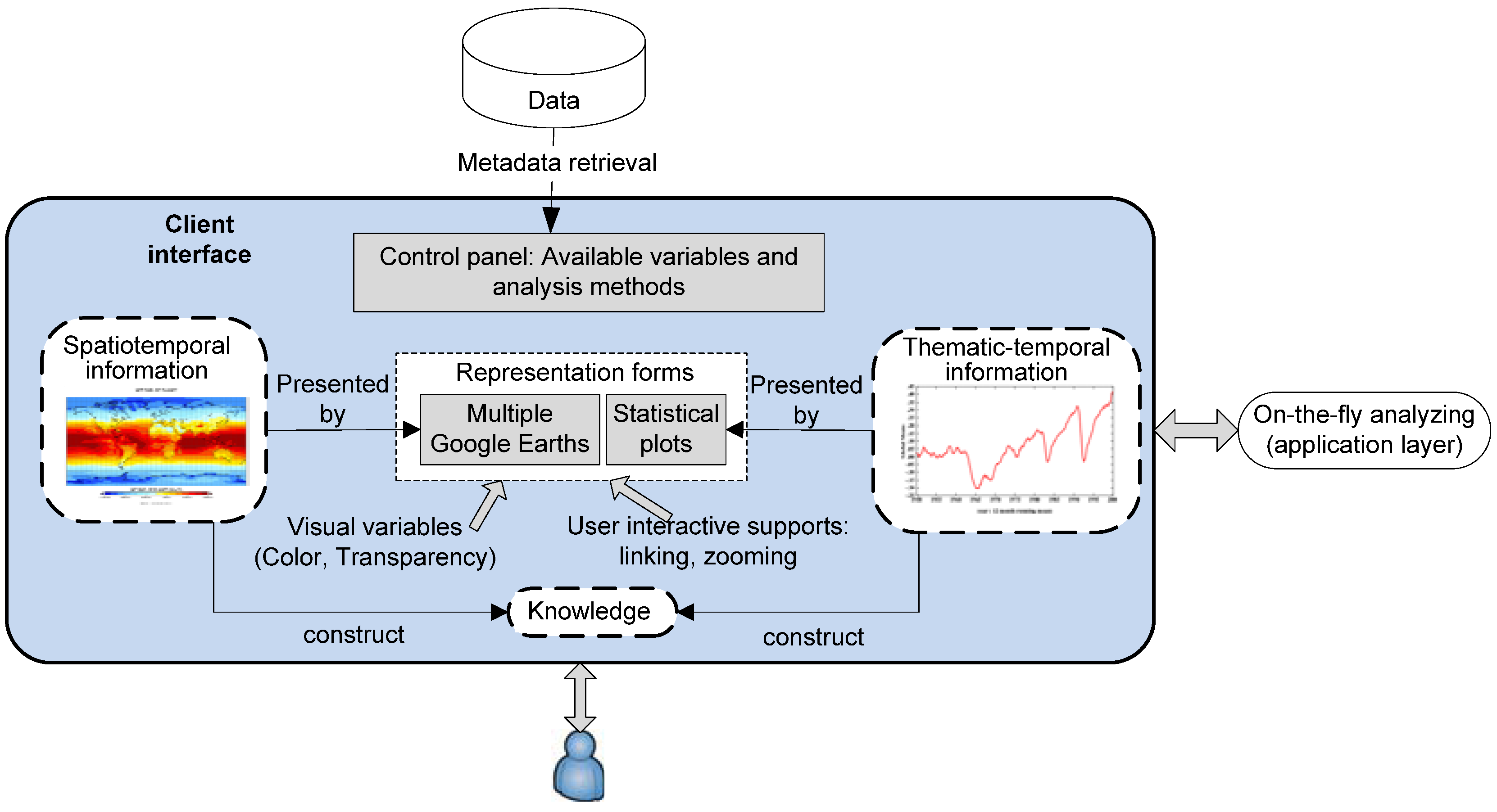
Figure 5 shows how the geovisual analytical tool performs for exploring climate data. When the user connects to the interface through a web browser, the client is automatically connected to the database. Information about data and function is initialized based on the metadata stored in the database and shown on the interface. Users can issue a request for visualization or analysis according to the available information. Based on the types of requests, different visual results such as images are returned and displayed as maps or statistical plots. Users can expose the underlying patterns of climate data through dynamic controls of visual results.
Figure 5.
Mechanism of geovisual analysis on the client side.
Figure 5.
Mechanism of geovisual analysis on the client side.
3.3.1. Map
There are two forms of data visual representations in this system: map and statistical plot. Flat maps are frequently used for climate studies. Meanwhile, 3D globe displays has the advantage in providing more intuitive view about the global location and other information which may be useful for climate study (e.g., terrain) [
24,
38]. However, this paper will not evaluate the trade-off between flat maps and 3D globes. Therefore, both are integrated into the system. Due to the advanced capabilities in dynamically visualizing multidimensional geographical data online, Google Map and Google Earth (GE) [
39] are selected for displaying maps of climate data at the client side. Instead of using one map as other climate analysis tools, e.g., VISUS [
24], maps can be attached to as many as six windows. Users can compare variables in parallel to acquire knowledge of spatiotemporal patterns. Moreover, all map operations on the six windows are linked together so that all map events occur on six windows synchronously. The map views presented in front of users are always focused on the same area. With comparison during view changes, users can find, for example, that one variable has high value close to the Equator and low value near polar areas and that another variable has an opposite behavior.
Besides providing static views of maps, the web client also supports temporal animated maps which can help detect the continuous dominant patterns through time [
40,
41]. If users conduct animations on multiple map windows, they will obtain the general spatial patterns showing how different variables change over the same time period. For example, from 1960s to 1990s, land surface temperature increases and the largest change appear around polar areas. At the same time, vegetation coverage decreases correspondingly, but the biggest change is found at places close to the Equator.
In addition, some widgets are provided for better making maps such as setting transparent colors for image layers in maps so that many layers presenting different information can be overlaid together.
3.3.2. Statistical Plots
Besides displaying maps of climate variables, the system is able to return the statistical results as statistical plots to the client. These statistical results are derived from the initial statistics or interactive statistics through user operations. In the case of initial statics, static graphs are usually generated to provide the description of data. Dynamic statistical plots are suggested if data analysts want to manipulate elements on the plots during the analysis, for example, the analysis of Albedo, which is described in [
42]. In the context of climate modeling, the model configurations (e.g., model inputs) are also taken into account as a part of statistical analysis. This will be further illustrated in
Section 4. Due to the nature of interactive manipulation, dynamic statistical plots are directly linked to the knowledge discovery process.
4. Case Study and Result
In order to illustrate the capabilities of our system, we use simulated data from GISS ModelE as an example.
4.1. ModelE Simulation and Customized Geovisual Analytical System
ModelE is a general circulation model (GCM) developed by NASA GISS. The model provides the ability to simulate many different Earth system parameters including interactive atmospheric chemistry, aerosols, carbon cycle and other tracers, as well as the standard atmosphere, ocean, sea ice and land surface components [
11]. Relevant model experiments and results have been submitted as part of the Coupled Model Intercomparison Project (CMIP) [
31]. Recently, we conducted 300 model runs with an 11-year simulation period for near-present boundary conditions using NASA and George Mason University cloud computing infrastructure in a spatial cloud computing fashion [
43]. ModelE simulates more than 300 variables on a global scale. The spatial resolution is 4 degrees in latitude and 5 degrees in longitude. The selected outputs for these simulations were monthly binary data with a size of 16 MB. All data have been transferred into NetCDF files. The total volume of the NetCDF data is around 750 GB.
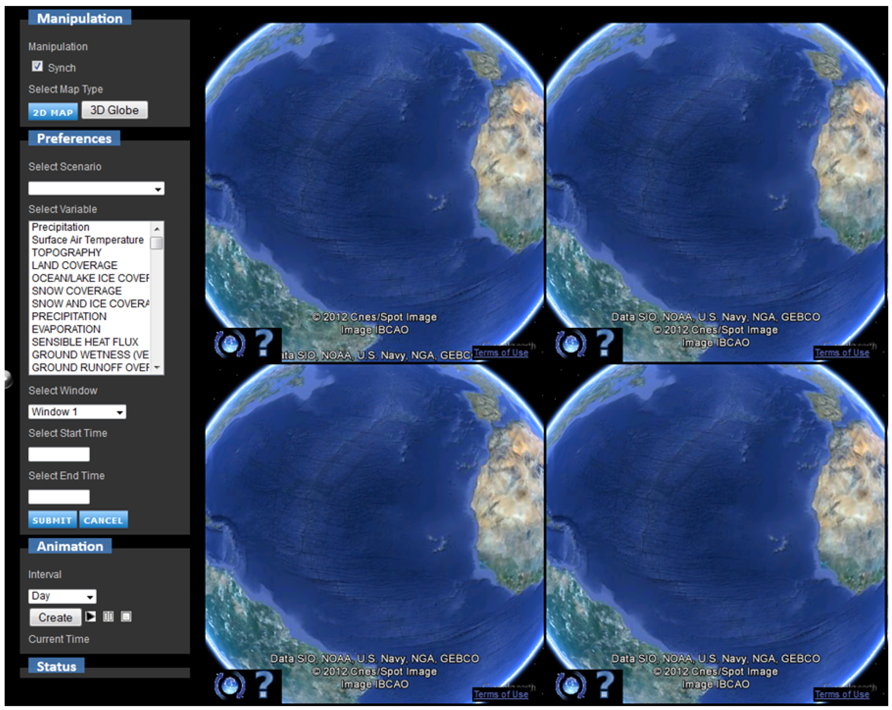
The available variables ready for use in the database is listed in the control panel on the left column of the client (
Figure 6).
Figure 6.
System interface: End users can use the GUI (Graphical User Interface) to select the parameters, time, and region, to be reviewed at a specific window. Multiple windows (up to six and with four shown) can be synchronized as needed for comparison.
Figure 6.
System interface: End users can use the GUI (Graphical User Interface) to select the parameters, time, and region, to be reviewed at a specific window. Multiple windows (up to six and with four shown) can be synchronized as needed for comparison.
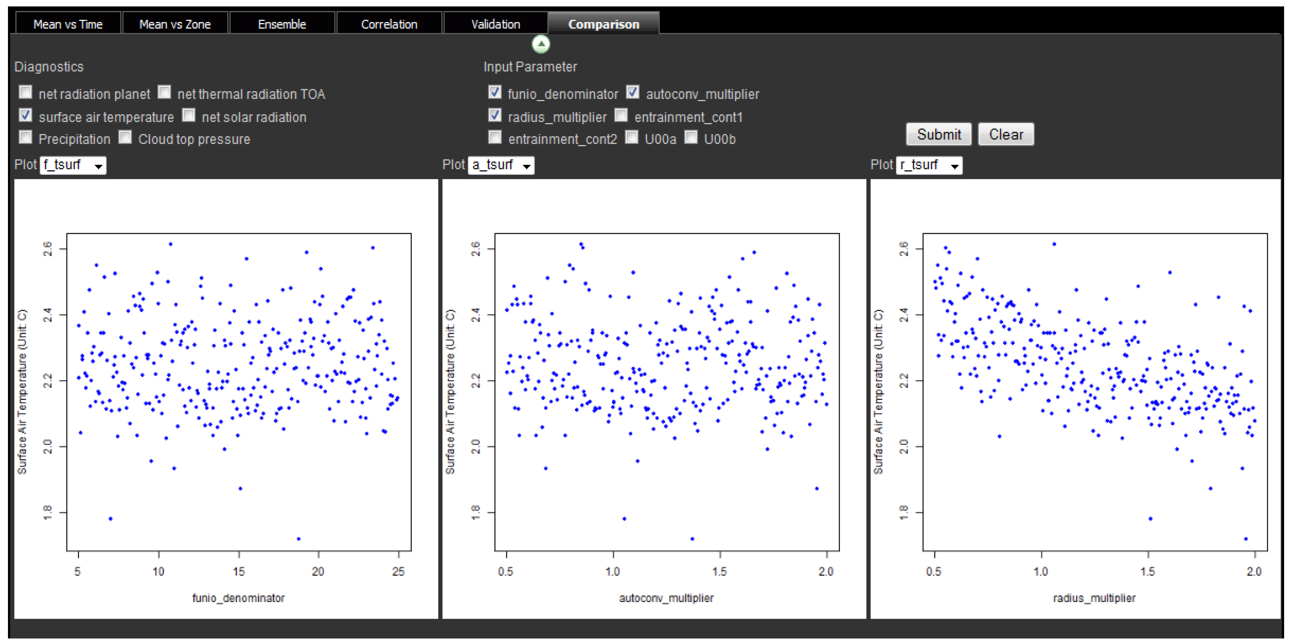
According to requests from scientists who use ModelE simulation, the initially-designed data analysis functions includes: (a) global and zonal mean based on month, season, year and 5-year; (b) ensemble mean and standard deviation; (c) relation between selected pairs of variables in scatter plot; (d) relation between input condition and output variable in scatter plot; (e) an assessment of the quality of the simulations as expressed in Taylor Diagram [
28]. The interface for interacting with the server-side analysis functions are revised according to the available functions. All proposed map functions in
Section 3.3 are usable for ModelE data. Users can define the input and see the output of statistical analysis through the panel on the bottom of the client.
4.2. Examples of Data Exploration with the Geovisual Analytical System
4.2.1. Detecting Spatial Variations of Multiple Variables Using Maps
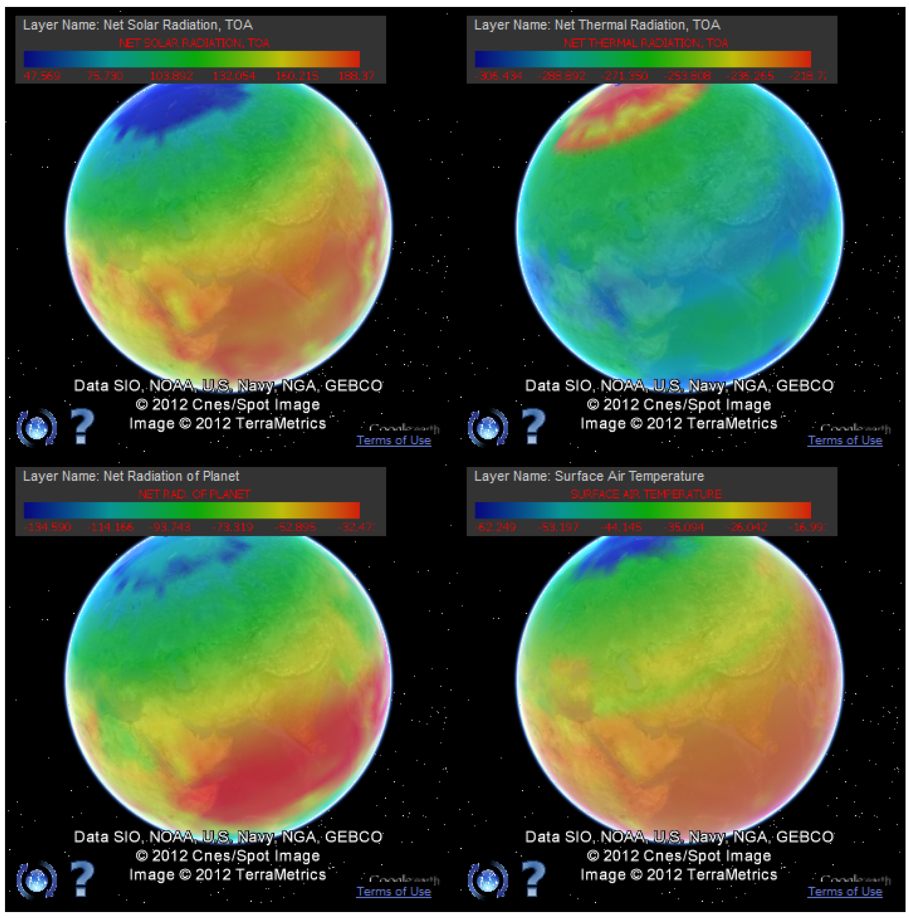
Spatial variations can be detected from maps showing mean values over geographical region. The ensemble means of 5-year annual mean (1956–1960) from 300 model runs are used for analyzing spatial variation in this experiment. Four highly related variables including net thermal radiation at the top of the atmosphere (TOA) (trnf), net solar radiation at TOA (srnf), net radiation of planet at TOA (net_rad_planet) and surface air temperature (tsurf) are selected as examples from the control panel and added into four different maps (
Figure 7). By comparing the four maps through synchronized map operations, we can find that srnf, turf and tsurf have high values within medium latitude area, but net_rad_planet has high values at mid-latitudes. Both net_rad_planet and srnf have obviously high value clusters over tropical ocean areas, but the values of tsurf evenly distribute along latitude belts and decrease towards the poles.
Figure 7.
Data exploration on multiple Google Earths (GEs).
Figure 7.
Data exploration on multiple Google Earths (GEs).
4.2.2. Advanced Analysis on Temporal Patterns
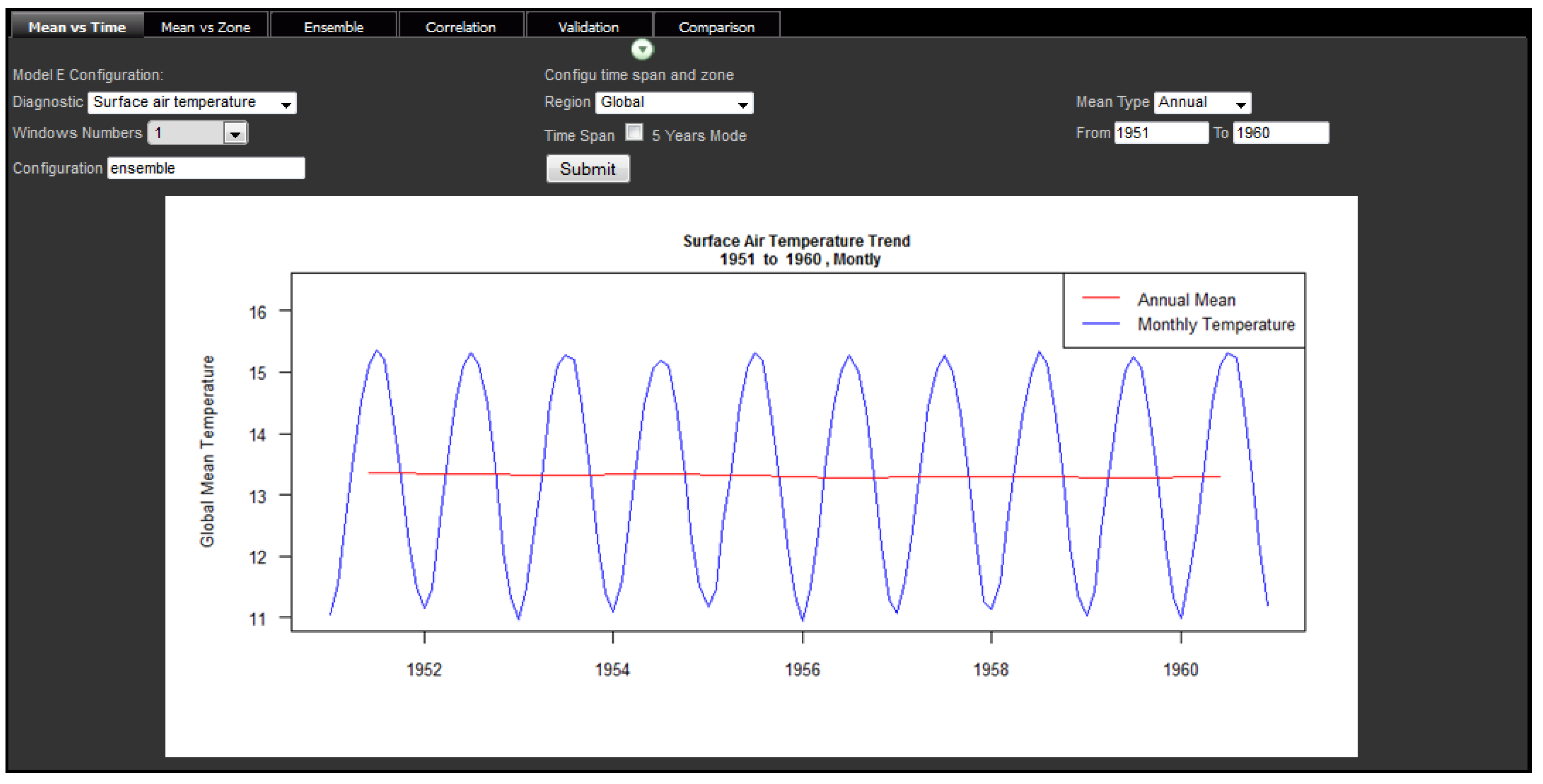
Maps are used to view the spatial variations whereas temporal variations can be detected more clearly from time series analysis (
Figure 8). The global mean of surface air temperature (tsurf) of a single run is used as the example. In the line plot, the blue line represents the change of monthly values and the red line represents annual mean values. We find a flat slope on the trend of the annual mean values which is unsurprising given the model simulation configuration.
Figure 8.
Interactive plot of mean values of a climate parameter vs. time using ensemble mean of surface air temperature as an example.
Figure 8.
Interactive plot of mean values of a climate parameter vs. time using ensemble mean of surface air temperature as an example.
4.2.3. Model Validation between Simulation and Observations
An important task of climate modeling is to evaluate the accuracy of the model. The evaluation against observations can be achieved in many ways. Often simple map differences are informative, but a compact way of representing spatial correlations and RMS errors is via a Taylor diagram. The first method retrieves data from the database directly and visualizes data on GE as two layers. Users can generally observe the difference between two layers by toggling operations and transparent color settings. Taylor diagram is calculated at the server side.
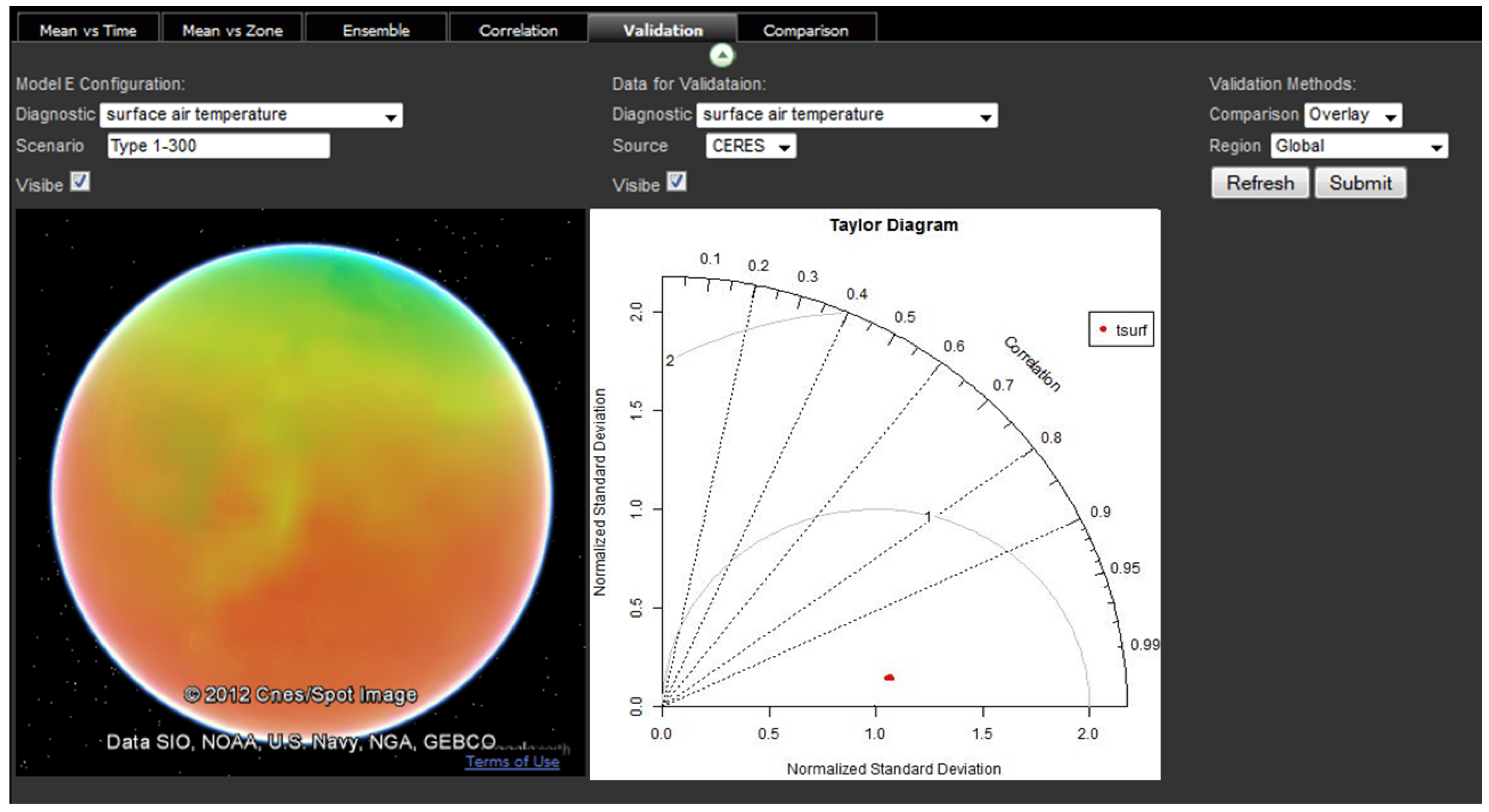
Figure 9 shows the interface for conducting quality evaluation and the resulting map and Taylor diagram. The evaluation is based on global 5-year mean values of surface air temperature from 300 model runs. In the returned Taylor diagram, all 300 values locate within the 0.5 RMS error contour and with greater than 0.95 spatial correlation [a perfect simulation would be represented by a point at coordinates (1,0)]. This result illustrates that the simulated climate condition is very similar to the observations.
Figure 9.
Client interface for evaluating the quality of simulation and the result of evaluation.
Figure 9.
Client interface for evaluating the quality of simulation and the result of evaluation.
4.3. Performance Evaluation
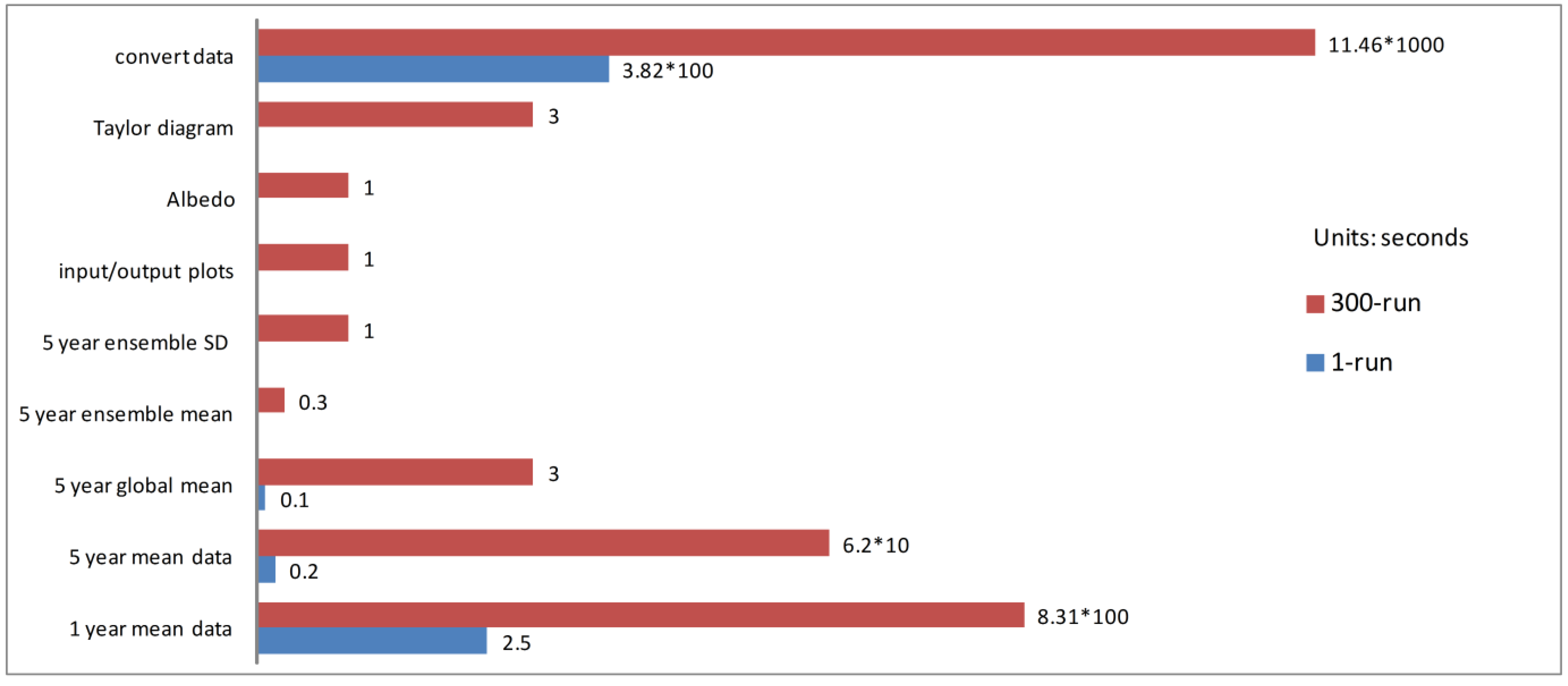
In order to evaluate the performance of our system, we record the time spent on various components in the process of data preparation and analysis (
Figure 11). We process data and record the time on a server with 12 core/2.88Hz CPU and 96GB memory. The computations include 1-year annual mean, 5-year annual mean, global mean of 5-year annual mean, ensemble mean of 5-year annual mean, ensemble standard deviation of 5-year annual mean, scatter plot for model input configuration and output variables, scatter plot for Albedo analysis (
i.e., scatter plot between thermal outgoing radiation and solar absorbed radiation), and Taylor diagram. Time is recorded respectively for data both from 1 model run and 300 model runs. As expected, the most time is spent on calculating 1-year annual mean and 5-year annual mean. The time used for calculating five 1-year annual mean values from 1956 to 1960 for data in 300 model runs can reach 831 seconds. By contrast, the time spent on the other analyses is only several seconds which is tolerable.
Therefore, storing initial statistics like 1-year annual mean is necessary. It is impossible for users to calculate 1-year annual mean repeatedly in every analysis. But whether 5-year annual mean and its global mean should be pre-stored in the data repository depends on the frequency of data access from users.
Figure 11.
Time for performing different statistical analyses.
Figure 11.
Time for performing different statistical analyses.
5. Conclusions
Data generated from climate models are large and complex. Distributed data users require a web-based environment to process climate data that are generated and stored in distributed computing resources. This paper describes a web-based geovisual analytical system for visualizing and analyzing climate data. The data from ModelE are used to demonstrate the efficiency of the system.
The system includes three components which are client, application server and database. These three components are integrated to support climate data archiving, processing, analysis and visualization. Multiple maps and geovisual exploratory techniques on the client side can help users conduct simple pattern detection and control advanced statistical analysis on demand.
Whereas the system is an initial step in the development of the web-based geovisual analytical system for exploring climate data, we will continue to improve the system with: (1) efficient management strategies for ultrascale data sets; (2) more initial statistics pre-calculated by considering both processing time and access frequency; (3) functions to process observation data retrieved from other vendors; (4) data analysis module for integrating analytical functions according to the requirements of climate researchers such as calculating differences between parameters; and (5) multiple visualization functions on the client such as dynamic plots for analytical results and dynamic symbol control for variables on maps.

 ,
, 