
Deducing Energy Consumer Behavior from Smart Meter Data †


1
The Mærsk Mc-Kinney Møller Institute, University of Southern Denmark, 5230 Odense, Denmark
2
Department of Engineering, Aarhus University, 8200 Aarhus, Denmark
*
Author to whom correspondence should be addressed.
†
This paper is an extended version of our paper published in IEEE International Conference on Smart Grid Communications (SmartGridComm), 2016, under title: Presenting User Behavior from Main Meter Data.
Future Internet 2017, 9(3), 29; https://doi.org/10.3390/fi9030029
Submission received: 2 June 2017
/
Revised: 23 June 2017
/
Accepted: 26 June 2017
/
Published: 6 July 2017
Abstract
:The ongoing upgrade of electricity meters to smart ones has opened a new market of intelligent services to analyze the recorded meter data. This paper introduces an open architecture and a unified framework for deducing user behavior from its smart main electricity meter data and presenting the results in a natural language. The framework allows a fast exploration and integration of a variety of machine learning algorithms combined with data recovery mechanisms for improving the recognition’s accuracy. Consequently, the framework generates natural language reports of the user’s behavior from the recognized home appliances. The framework uses open standard interfaces for exchanging data. The framework has been validated through comprehensive experiments that are related to an European Smart Grid project.
1. Introduction
The deployment of smart electricity main meters for households has been tremendously growing in the last few years. For instance, China has nearly 210 million units installed [1], the United States (US) has already deployed more than 60 million meters [2], and the European Union (EU) is planning to replace at least 72% of the household electricity meters by 2020 (around 200 million smart meters will be deployed) [3]. Meters are not only used to provide electricity billing but also to deliver value-added services to the power grid. Such services are developed to provide energy utility with diagnostic information about the distribution grid [4,5] or by permitting third-party application providers to deliver grid-related information services to residential homes [6].
Consequently, several types of research make use of the provided meter data and apply machine learning algorithms to it [7,8]. Such algorithms are called Non-Intrusive Load Monitoring (NILM) algorithms and aim to disaggregate loads for individual appliances from the total power consumption data. Numerous NILM techniques are proposed in the literature [9]. In this context, the computer-aided design should be fruitfully applied to support load disaggregation algorithms as well as to combine them with different techniques to achieve better detection results and present the analyzed results in a user-friendly manner.
This work rests on recent advancements in NILM based on smart meter data readings, data recovery mechanisms and model-to-text transformation techniques for presenting the final results in a user-friendly way. We propose a framework for deducing the user’s behavior from the electricity usage fingerprints resulting from activities in the residential home. Figure 1 shows the conceptual architecture of the proposed framework; numerical labels are used to show the items to be explained. Initially, the power signature of each home appliance is measured individually by the main meter and stored in a shared database; the database is called DataBase Cloud Service (DBCS) [10]. The stored signatures will be used in the training of the NILM algorithms. NILM algorithm will look for such signatures in the aggregated meter data of the overall household consumption. However, such aggregated data may be faulty due to communication and/or computation inefficiencies. Therefore, quality check of the aggregated data is necessary (Label 1). In case of poor data quality, data recovery mechanisms are used to fix the aggregated data (Label 2). The recovered data is then stored in the DBCS and Non-Intrusive Load Monitoring (NILM) algorithms are applied to deduce the used appliances from the data (Label 3). The results of the algorithms will subsequently be stored in the DBCS. However, the disaggregation results are fallible due to the effect of the noise in the transmission lines and the energy consumption of unknown appliances. Therefore, outcome refinement step (Label 4) is used to observe common energy consumption pattern between multiple homes. The result of this process is appliance usage pattern, that can be used by the service providers to derive various statistical properties. Finally, for making the results comprehensible to the end-users, a natural language generator tool (Label 5) is developed to convert the processed data into textual Human-readable reports.
The key novelty of our research comes from the combination of data recovery mechanisms, machine-learning techniques for event recognition with a subsequent analysis and translation of information into natural language. After an initial training period, the responses to the actual user behavior can be delivered in near real-time. The immediate benefit of the proposed framework stems from the fact that an observer no longer needs to be a skilled technician but instead can rely on comprehensible reports on user behavior. For instance, in the telemedicine domain, the doctors can remotely observe the behavior of their patients and in energy domain, energy utilities may use such reports to evaluate their customers (e.g., demand response programs).
The contribution of this work is a generic framework for deducing and presenting users behavior from their smart meter data. The framework aims to:
- separate disaggregation data analyses from data representations;
- use open standard interfaces to exchange data (i.e., ZigBee and RESTful web interfaces) in a seamless way;
- provide a unique and shared database for appliance signatures and disaggregated results;
- improve the aggregated data quality by detecting and fixing its errors;
- combine the consumptions of several homes to detect appliance usage patterns.
- provide natural language reports about the user behavior to relevant stakeholders (hospitals, companies, etc.).
The paper is structured as follows: Section 2 gives a brief overview of the related work. Section 3 shows the techniques and modeling languages used in this work. Section 4 presents the proposed framework and Section 5 demonstrates the applicability of the framework from a test case. Section 6 draws a conclusion and outlines future work.
2. State of the Art
While frameworks for Non-Intrusive Load Monitoring (NILM) by smart meter power consumption data forms a relatively new research field, diverse algorithms and tools have been presented to implement these frameworks. For instance, NILM-Toolkit (NILMTK) [11] is a framework aims to evaluate NILM solutions. It supports a broad range of known datasets that can be used to train or validate an algorithm. It comes with two benchmark algorithms to compare a new algorithm against. The NILMTK will help researchers to easily share and compare algorithms [11]. Another framework to accomplish better comparison and sharing is the NILM-eval framework. It is based on Matlab and supports algorithms to be written in either Matlab or Python. The NILM-eval and the NILMTK are created to solve the same problem and compatible with each other since their interfaces are the same [12]. Besides the simplicity stemming from only using smart meter data, research has also focused on the use of data with low time resolution in terms of seconds. Ruzzelli et al. in [13] present a smart system for recognition of electrical appliance activities in real-time. The proposed system provides accuracy in determining the set of appliances being used. However, Liao et al. in [14] rely on data collected at Hz, and they achieved a precision of in detecting switching events. Chiang et al. in [15] present a load disaggregation technique that uses harmonic frequency signatures of appliances. Their technique allows to disaggregate the loads in a very short time (a quarter of a second) since it does not wait for appliance state change, as it was done in previous approach, and it monitors directly the frequency signatures.
Data quality is an area that recently has become a hot topic due to the large quantity of data. Geographic information, a field that deals with citizen data and used for maps, weather prediction and climate research, comes up with several ways of describing quality in spatial data [16] and methods for defining quality in time series data [17]. Data quality may vary due to some facts, on the one hand, network suitability and the test equipment faults may cause gaps in the collected datasets and that significantly effect its quality. One way to deal with such gaps is to use mathematical gap filling techniques to come with a qualified guess on how the data would look like in the gap [18]. However, if the signal is so stochastic, the gap filling is not recommended [19]. On the other hand, power line noise may add a layer of random data into the datasets [20]. Digital filters are commonly used to solve this problem [21]. However, many researchers strive to make tools that can better analyze data quality in different areas. In the area of spatial data, a tool named “Quality and Workflow” [22] is developed to help researchers to select the best-suited data for a given data-driven project. It does this by looking at different quality criteria, given by the user or found in standards for spatial data. In the area of bioinformatics, a tool named QCScreen [23] is developed to help creating better dataset to metabolomics studies. In metabolomics studies, the datasets often created by joining information from several different experiments of various quality.
In order to store and share datasets, seamless interfaces are desired by the smart grid research community. Jacobsen et al. in [24] define a service-oriented architecture for the collection of electricity data from resource constrained devices in residential homes. It presents the requirements for open protocols, privacy, security, and scalability, leading to usage of ZigBee and IPv6 over Low power Wireless Personal Area Networks (6LoWPAN). In the same work, the REpresentational State Transfer (REST) principle is applied when designing a database cloud service and application layer protocols, providing storage for other elements in the architecture.
Finally, generation of natural language reports from software models is considered to be a key target to present the energy data in human-readable reports. Burden et al. in [25] investigate the possibilities to generate natural language text from Unified Modeling Language (UML) diagrams. They use a static diagram (i.e., class diagram) transformed into an intermediate linguistic model to demonstrate their approach. They show that the generated texts are grammatically correct.
3. Background
This section gives a brief overview of data reconstruction, appliances detecting algorithms, interfaces and natural language generators that are used in this work.
3.1. Quality Check
The ISO 8402 standard describes the data quality as: The totality of characteristics of an entity that bear upon its ability to satisfy stated and implied needs [26]. However, the data quality is very depended on the intended application and is, therefore, hard to generalize. Tools such as Quality and Workflow tool [22], QCScreen [23], and NILM-Toolkit [11] are built to analyze the data and help researchers to select the best-suited data for a given dataset.
3.2. Gap Filling
However, gaps can appear in datasets due to communication errors or faulty devices and can significantly degrade the data quality. Therefore, various algorithms have been developed for filling the gaps such as Papoulis-Gerchberg, Wiener, Spatio-Temporal, Envelope, and Empirical Mode Decomposition Fillings.
3.3. Load Disaggregation Algorithm
The Load Disaggregation Algorithm (LDA) is defined as an algorithm that takes data on aggregated electricity loads from multiple appliances, as input, and outputs disaggregated loads for individual appliances [27]. Combining LDA with a non-intrusive approach to obtain data, it forms a method for NILM. Assuming that labels with information about appliance loads are available for some of the load data, the problem of disaggregation is similar to a supervised learning problem known from Machine Learning (ML) or a problem of statistical regression [27].
There are generality two approaches to pattern recognition: supervised and non-supervised. In supervised training it is assumed that the ground truth of your system is known. For a NILM application this means that the true consumption of the appliances needs to be available for the training process. This means that sub-meters must be placed to measure the appliances individually, which often is costly and time consuming. In non-supervised methods only the main meter readings are available, and no information about the appliances are known. This type of algorithms will usually try to cluster the readings in distinct groups cosponsoring to a guess of what appliances that correspond to the reading.
3.4. Outcome Refinement
When an appliance is in an environment with a lot of background consumption, some of the background consumption can be interpreted as the appliance. This appliance interference creates a scenario where it seems like the appliance is used more than it actually is. By improving the method with the knowledge of how a specific appliance is most commonly used, also called the norm usage, it is possible to filter the signal and improve the performance. Therefore, we defined a filter called Norm Filter, it is a filter enforces the normal behavior of a system. It filters out events that are unrealistic given some normal behavior.
3.5. Data Representation
The section gives an overview about the main components that are used to build software applications that are capable to present data in human-readable reports.
3.5.1. Modeling
UML [28] is a standardized general-purpose modeling language in the field of object-oriented software engineering and standardized by the Object Management Group (OMG). It includes a set of graphic notation techniques to create visual models of object-oriented software-intensive systems. UML semantics can be extended by the concept of profile. UML 2.x has 14 types of diagrams divided into two categories. Structural diagrams emphasize the components which must be present in the system being modeled (e.g., Class, Deployment and Profile diagrams). Behavioral diagrams emphasize the behavior of the system being modeled (e.g., State machine, Activity and Sequence diagrams). For instance, the relationship between a user and home appliances are depicted in static diagrams and the interactions between that user and the appliances are depicted via behavioral diagrams. Model-to-Text is an Eclipse project that is concerned with the generation of textual artifacts from high-level models such as UML models. In addition, OMG specifies a correlated language named Mode-to-Text Language (MTL) to express its transformation. Acceleo [29], an Eclipse plug-in tool, is a pragmatic implementation of the MTL standard. It is widely used by software engineers to generate code from high-level models [30].
3.5.2. Interfaces
REpresentational State Transfer (REST) is a design style for designing application based on web services, calling for simple (client-server, stateless, self-documenting) interfaces building on Hyper Text Transfer Protocol (HTTP). The openness, modularity, interoperability and security provided by REST are beneficial when designing interfaces for an open framework such as the proposed. Therefore, RESTful interfaces provide seamless interaction between applications that assures the separation of the framework’s concerns.
The ZigBee wireless interface, implemented by ZigBee Alliance [31], is developed on the top of the IEEE 802.15.4 radio standard. It is widely used in home automation applications, offering low transmission rates over low-power wireless radio links. However, ZigBee networks are lacking reliability due to interference, noise and other radio link impairments. Therefore, ZigBee’s mesh networks are used to compensate such lack.
4. Proposed Framework
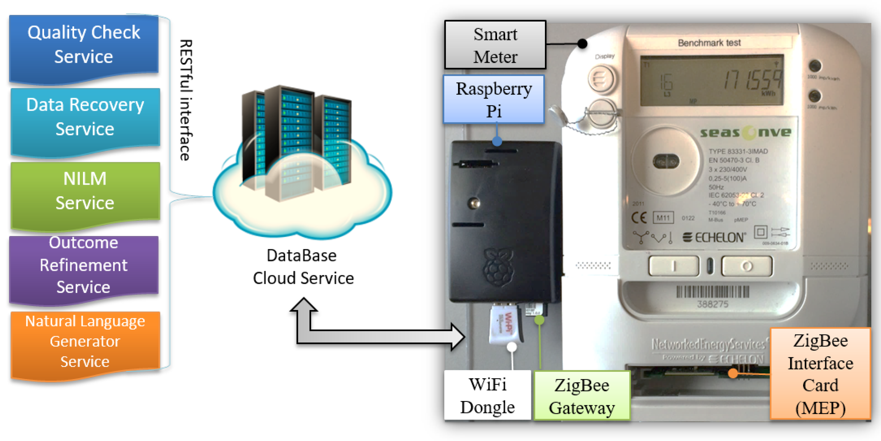
In this section, the context of the framework is outlined and its elements are defined. The framework’s conceptual view is outlined in Figure 1 and explained briefly in Section 1. To complement, Figure 2 shows the real implementation of the framework. The framework consists of Echelon electricity meter with ZigBee interface card called Multipurpose Expansion Port (MEP) card, developed by Develco Products company and a Raspberry Pi that pairs with the MEP card via ZigBee gateway that is connected to it. The Raspberry Pi works as a gateway and data handler. It forwards the measurements to the developed DataBase Cloud Service (DBCS) [10].
The context is that a user is living in his/her home and there are some electrical appliances are installed in the home. When a user makes use of an appliance, it is referred to as a usage. The framework gathers the user’s consumption data from the smart main meter and then tries to check and recover the data and then recognize which appliances were used with their usage time. The framework interprets the results and builds a natural language report of the user’s behavior. The framework’s beneficiaries will receive natural language reports (e.g., via emails, SMS, social networks, etc.) about the observed users’ behavior and thus they do not have to be physically present to the users.
The data check, data recovery, LDA, outcome refinement, and Natural Language Processing (NLP) are deployed as services in the intelligent services part, and they use RESTful interface to exchange data. Due to this interface, the framework enables an easy upgrading to its services without affecting other components in the framework. The following sections explains how each service is working.
4.1. Data Quality Service
This service aims at check the quality of the aggregated meter data. It checks the data against two quality parameters; sample availability and activity.
4.1.1. Sample availability
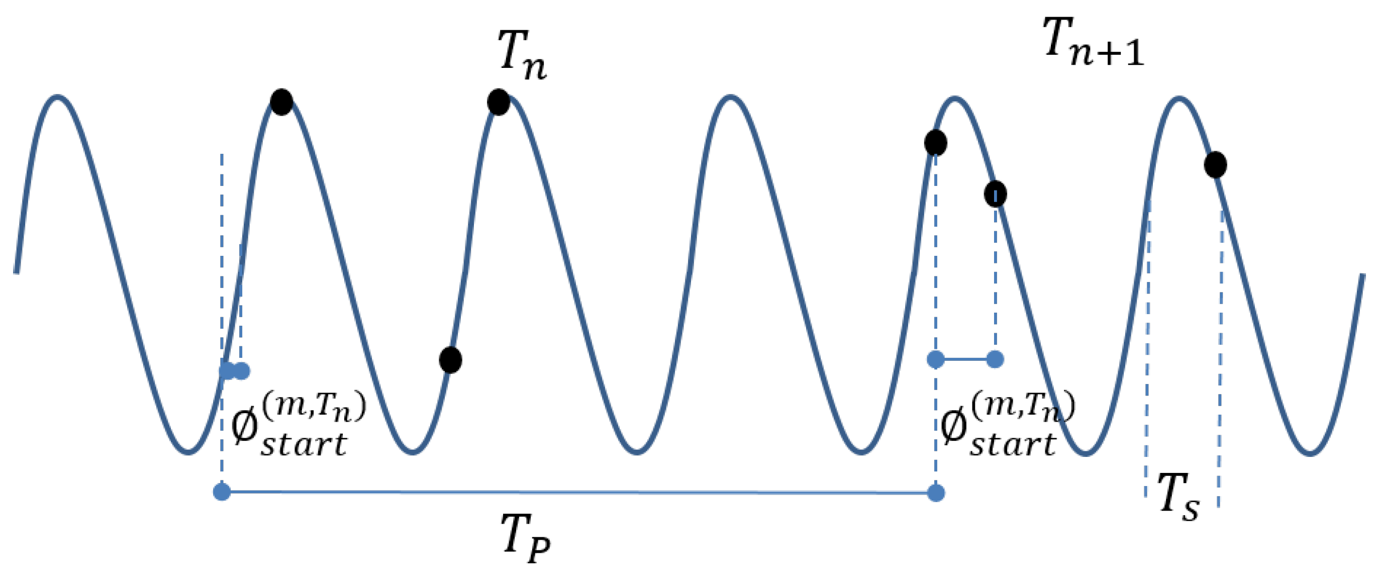
It is defined as the amount of samples observed in a time slot over the expected amount of sample. To calculate the amount of samples expected to be in a specific period of time , where is a specific period of time for a specific meter m, the sample phase for the given period needs to be known. Figure 3 shows an illustration of a signal, the black dots are the samples and the big red dots are the ones that are missing. The sample phase is the time from the beginning of the period to the first expected sample. This is needed since for a timeslot of a length of can the maximum expected sample amount vary with 1. This is shown in Figure 3 where the period has a potential of 11 samples, whereas period only can have 10.
As shown in Equation (1), the maximum number of samples for a meter m in the period calculated by taking the period time , corrected with the sample phase for the given period, and dividing it with the sample time . The sample availability quality of the meter is calculated as the ratio of observed samples in the timeslot to the maximum samples, shown in Equation (2).
To inspect the quality of the collected data in a given period , that have a set of meters with a cardinality of M, we took the mean value of all the meter quality’s, as shown in Equation (3).
A quality vector Q is constructed for each house. The quality vector contains the house quality found with a period in one hour.
4.1.2. Activity
It is measured as a change in the signal from prior values. Since the meter data is intended for appliance recognition, it is of interest where in the data there is activity and where not. Both areas are important for a NILM application in training scenarios. Equation (5) shows the definition of an area of data where there is a change in it.
where describes a threshold to filter out changes caused by noise. This can also be described as the standard deviation over an area is greater than the threshold.
4.2. Gap Filling Service
Gaps in datasets lower its quality and one way to deal with this problem is by using mathematical gap filling techniques. Gap filling algorithms have different approaches to deal with the data. Some algorithms deal with frequency spectra, for others jitter power or the exact sample value they are trying to estimate. Some algorithms have also been designed for small gaps, while others have been designed for larger.
In this work, five popular algorithms for gap filling have been chosen and will be explained in the following sections.
4.2.1. Papoulis-Gerchberg Algorithm
The P-G algorithm is a multi-gap filling algorithm, meaning it is capable of correcting more than one gap at the time. This makes the algorithm perform good in conditions with many gaps and few available data points between gaps. This is due to its ability to collect information about the signal across multiple gaps [32]. The P-G algorithm works under the assumption that the signal is a periodic stationary signal with a known bandwidth. The signal will, therefore, consists of frequency components, and everything outside the band is assumed to be noise.
The true bandwidth is also unknown in the signal. The P-G algorithm is very depended on the bandwidth for a correct reconstruction. A modified version of the algorithm that estimates the bandwidth, by varying the frequency components and analyzing the mean square error on the known signal is therefore used [33]. This approach is fairly good at estimating the true value of , but is time-consuming. The implementation of the algorithm used in this work can be found in [34].
4.2.2. Wiener Filling Algorithm
The Wiener filling algorithm is an extension of a Wiener predictor. The Wiener predictor assumes that there exist a linear relationship between the next sample and the previous samples. By trying to predict the missing samples from both sides of the gap, and combining the results, it estimates the missing samples [35]. For larger gaps, this method relies on earlier predictions to close the gaps. This result in errors being accumulated over the gaps. The method is fast and is therefore suited for large data with small gaps. The implementation of the algorithm used in this work can be found in [36].
4.2.3. Spatio-Temporal Filling Algorithm
It uses singular spectrum analysis to split the signal into a series of sub-signals. The sum of the sub-signals is the original signal. The sub-signals are ordered so the most dominant is first, and the least dominant is last. The reconstruction philosophy is that the gap has introduced noise in the signal, but a sum of only the most dominant sub-signals must be close to the original signal without noise. However, to know how many sub-signals to include in this sum, we introduce another artificial gap. While the sub-signals are being accumulated the mean square error of the artificial gap is observed. When this mean square error hits its minimum peak, it is assumed that the reconstruction is as good as possible [37]. This method is very popular for gap filling. It has shown to be very noise resistant since it finds the overall trends in the data. It does require quite a lot of data to be known post and prior to the gap since an artificial gap must be introduced. It is based on singular spectrum analysis which assumes that the signal consists of stationary processes. This is a similar constraint to the P-G algorithm. The implementation of the algorithm used in this work can be found in [38].
4.2.4. Envelope Filling Algorithm
It depends on the expected power of the signals. Looking at the envelope of the signal it assumes that all local maxima and minima must lie on the upper and lower envelope. It looks at the data prior and post of the gap and try to estimate the number of local maxima and minima in the gap along with their locations. It does this by looking for patterns in the time series data [17]. When the new maxima and minima are found the points is connected by using spline [18]. The methods do not make any assumptions about the signals stationariness or bandwidth. The method can also be used on aperiodic time series. The implementation of the algorithm used in this work can be found in [39].
4.2.5. Empirical Mode Decomposition Filling Algorithm
It uses empirical mode decomposition, to break the signal into Intrinsic Mode Functions (IMF). The sum of all IMF’s is the original signal. The IMF’s is all lower frequent and simpler in structure than the original signal. The hypothesis is that it is easier fixing a gap in a simple signal than a complex one. The envelope filling algorithm is used to fix the gaps in the IMF’s. The IMF’s can now be accumulated to get the original fixed signal. Like the envelope filling algorithm does it not make any assumptions about the signals stationariness, bandwidth and can be used on none equally spaced time series. However, making an empirical mode decomposition on a signal with a gap in is a non-trivial process and can introduce errors [18]. The implementation of the algorithm used in this work can be found in [40].
4.3. Load Disaggregation Algorithm (LDA)
Load disaggregation and appliance recognition are some of the key aspects in Non-Intrusive Load Monitoring (NILM). The main purpose of the NILM approach is to better understand the power usage in the home. It also have the potential to help the different households to more optimal power savings. This is done by informing the residents about the power consumption of individual appliances. It is shown that informing a household about its usages pattern can lead to significant savings [41]. This makes the basis for load disaggregation, where appliance specific load is deduced based on the main meter load. This enables the user to know what uses the energy and when.
4.3.1. Concepts and Challenges
The aim of NILM is to partition the whole house consumption data into appliance specific consumption.
This can be seen as in Equation (6) where P(t) is the total consumption at time t, is the consumption of appliance n at time t, and L is the loss factor in the electricity lines. The aim is to partition P(t) back to the different appliance specific consumptions. In order to structure the problem we categorize the appliances in 4 groups [42]:
- Type-1: Appliances that only have 2 states corresponding to ON/OFF. This could be a lamp or a water boiler.
- Type-2: These are appliances with multiple states. The appliance in this category can be modeled as a finite state machine. Many modern devices such as TV’s, computers and washing machines fall in this category.
- Type-3: These appliances are referred to as “Continuously Variable Devices”. These devices have a variable power draw and is impossible to model as a finite state machine. This could be appliances like power drills, and dimmer lights. These are by far the hardest for the NILM algorithms to detect.
- Type-4: These are a special kind of appliances that are always ON and consume energy at a constant rate. Such devices could be smoke detectors and burglary alarms.
The appliances in Type-4 is not a particular researched area, since it does not give the user much information to calculate savings from. These appliances are often using very little energy.
Type-1 and Type-2 are commonly used, and can cover almost any appliance. In the area of event detection is the most common approach to see all appliances as Type-1 and detect ON/OFF events. Most appliances today is Type-2 due to the growing amount of complicated electronics that are embedded in them. There are devices that are Type-2 but most of the time act like Type-1 appliances. An example of this is the vacuum cleaner. On most vacuum cleaners, the user is able to change the suction intensity, which makes it Type-2. However, most people do not change this very often, so the energy usage looks more like a Type-1 appliance.
4.3.2. Features
For data disaggregation it is common to use method based on machine learning and optimization. The approach is to first extract features from the dataset, and then train or validate advanced statistical models by using these features. In NILM, the features can be sub categorized in steady state, transient state and non-traditional features.
Steady state features is features that can be extracted when the signal is in a stable state. Features that are often extracted in this state is “Power Change” which is the jump in power or reactive power usage. Time and frequency analysis is often used on the voltage and power signals of the meters. It is shown that analyzing the harmonics in signals is a powerful way of making appliance detection [43]. The trajectory between voltage and power usage is a good feature. This can be used to detect the reactive power of a signal of inductive loads. Some researchers have shown that different appliances makes different noise profiles on the main line. Unfortunately, this kind of recognition require a high sampling rate in the kHz or MHz area [44]. The transient state of an appliance is a short state that comes when an appliance switches between steady states. In this state, there often is appliance semi-unique waveforms in the current and voltage domain. The noise generated on the mainline in the transition is also a good indication of the appliances type. There also exists a series of non-traditional features that is used in special types of algorithms. One of them is based on matching the power usage profile to geometrical figures, and using the series of figures to recognize an appliance [42]. Many of the above features requires a high sample rate in kHz or MHz span in order to be effective. This kind of resolution is often not available since it is a normal smart meters that are providing the data. For a smart meter, a sample rate at 1 Hz would be considered fast, and for many applications this is down to 0.03 Hz or slower. It is, therefore, common only to use the steady state features, and most of the time only the power change feature, which looks at changes in power, reactive power, current or voltage.
4.3.3. Learning Strategy
When the features are extracted from the signal there are several algorithms that can be selected for the training process. They can roughly be split up in two categories optimization algorithms and pattern recognition algorithms. The optimization algorithms relies on a database of appliance info, and tries to find the subset of the database that is most likely to be in use.
This is illustrated in Equation (7) were a set of appliances that correspond to the measured signal ŷ needed to be found. This is achieved by searching the known database of all appliances . This is done by taking the powerset of the database and finding the subset that minimizes the error. It can therefore be seen as a minimization problem, where the desired set is the arguments to the minimum solution. This approach is fine for small amounts of appliances, but for large databases and many appliances in use at the same time this would take far too long to be practical.
Due to this, most researchers use pattern recognition techniques instead. These have the benefits of being more scalable, and be usable even if only parts of the device database is known. The basic concept is to create a statistical model that can be used to classify appliances. For this kind of training it is easy to collect a big training set, but it requires the groups to be manually labeled afterwards. Many algorithms are based on clustering techniques and Hidden Markov models (HMM) [42,43,44,45,46,47]. HMM have proven very effective when classifying Type-1 and Type-2 appliances. This is due to its ability to model state changes as an imported part of the classification. It is shown that using clustering techniques can greatly improve the classification, and reduce the training time. Artificial neural networks are also showing great promise, and is a topic that is currently in focus by many researchers [43].
4.3.4. Challenges
There are many challenges in NILM. One is the Type-3 appliances. Due to their varying, and at times random, energy consumption it is hard to fit them to a behavioral model. This is made further harder by the low sample rate. Many great features of the appliances is hidden due to the low sample rate most data is collected with [42]. Another problem is the top consumer’s problem. In a household there are some appliances that require a lot of energy when they are on, such as stoves, air conditioners and refrigerators. These are referred to as the top consumers. Then there are the appliances that consume very little energy like laptops, DVD players and routers. The top consumer’s problem is that the top consumers are so dominant that they make it hard to track the power signature of small consumers. This is why many researchers only focus on the top 10 consumers when during NILM applications [11].
4.3.5. Recognition Methods
Methods based on Hidden Markov Model (HMM) are a very popular method for NILM. Three methods are selected to be validated in this paper. The methods are selected since they are often referenced in the literature, and is often used for benchmarking. All of the algorithms are based on HMM or clustering in different configurations. The following subsections will briefly introduce the algorithms.
Factorial Hidden Markov Models
The HMM has proven to be one of the most used tools to create probabilistic models based on time series data. This is done by seeing the system as a series of observable states , and a series of hidden states [45]. It is assumed that there exists a probabilistic relation between the observations and a sequence of hidden states . This is implemented as a first order model, which implies that the current hidden state is only depended on the previously state and the current observed state . In NILM can the observed state be seen as the observed consumption as seen from the main meter. Where the hidden state can be the unknown consumption of an appliance.
The joint probability for a specific hidden state that has caused the observed output can be seen in Equation (8). is the emission probability, which shows the conditional probability for being outputted by a given hidden state . The probability for a state change is given by the transition property .
Factorial Hidden Markov Models (FHMM) [45] is an extension of this classic HMM where there exists several hidden state chains that all contribute to the observed output. This can be seen as an extension to Equation (8) where the hidden states can be seen as a set of states as shown on Equation (9) where is the number of chains.
As an extra constraint can each hidden state, in each chain, only depended on the previously state in the chain, and not on the hidden state of other chains. This makes the state transition probability to be defined as in Equation (10).
The observed stated is therefore created by the contribution of many different hidden states. In this implementation there is normally used only two or three states, since most appliances are seen as Type-1 or Type-2 appliances. One chain for each of the appliances plus one that is called the other chain is created in the model. The other chain is to allow for the other appliances that are not taken into the model and noise. The model can therefore be used to validate for a given output what is the probability that a given appliance is contributing to the output. The concrete implementation for this algorithm has been adapted from the NILMTK [11].
Parson
The Parson algorithm is a variant of the Kolter and Jaakkola algorithm [46]. The algorithm is designed to be a semi-supervised learning algorithms. This means that the algorithm does not need to train on the data from the concrete house prior to deployment, but it still requires some prior knowledge. The idea is to have a database of general appliance models that tells how specific appliances most likely will behave. This model will be able to detect the device, and do some unsupervised special training to better fit the concrete appliance.
The algorithm is based on a kind of HMM called “difference HMM” since they take the step difference in the data and use as the observed output . In a normal HMM there is only emitted one output for each hidden state in a chain. In the Parson algorithm the model is changed to output two states, and , from the hidden states.
The is corresponding to the step in power that is observed since the last sample. It is assumed that the only thing that can cause a step in power is if an appliance change states from one to another. The is the constant power consumption the appliance would have in the state. This is used to filter out the appliance if the power consumption observed is smaller than this threshold.
It is assumed that the power consumption of a state in the general model of an appliance can be modeled as a normal distribution. This can be illustrated as in Equation (11).
This shows how the power consumption of an appliance is modeled as a normal distribution. The step Power , can also be modeled as a normal distribution that is created from the change between two states as shown in Equation (12).
To model the constraint that the meter only can be on if the power consumption present in the signal is higher than the requirement for the state is an additional constraint added to the emission probability. This constraint is mathematically described in Equation (13).
where is the measured power consumption and is the appliance power consumption constraint. This makes the probability going towards zero if the total power draw is too little and towards 1 if there is more than enough power. This is a loose constraint since too high power draw also could be created by other appliances. To minimize the impact this have for the algorithm is the mean power draw subtracted from the data before searching for other appliances.
In the implementation validated in this paper are all appliances modeled as Type-1. The algorithm is allowed to train on the house data, to better fit the general models to the appliances and create the initial database.
Weiss
The algorithm proposed by Weiss called “AppliSense” is another approach that does not use Markov models [47]. The philosophy is that some appliances like lamps and kettles are purely resistive, where others like washing machines and air conditions are more inductive and some appliances like laptops are more capacitive. By measuring not only the power consumption, but also the amount of reactive power it is revealed if there is inductive or capacitive appliances.
The algorithm is supervised since it requires a signature database to be created prior to usage. The signature database consists of how the changes will be in reactive and real power for a specific device when it is turned ON and OFF. In their paper, the authors show a method where this database can be created of a user, by using a smart-phone application and turning ON and OFF appliances in the house, and inputting the information in the mobile application [47]. In this paper the database is created by data collected from the sub-meters measuring only the devices.
The algorithm looks for significant power changes in the data. If a change is found it is assumed to be an ON or OFF event. The change is now compared to all the values in the database. If a close match is found it is assumed to be this device, if not it is an unknown device. This limits the approach to Type-1 appliances, and the algorithm requires the reactive power to be measured.
4.4. Outcome Refinement Service
Not just the sample rate and error rate are determining factors when designing a NILM application. The environment, in which the application is deployed and trained, is critical for the performance of the system. The environment contains the parameters describing the static conditions of the household which the algorithms are deployed in. An example of an environment parameter can be the number of known devices, the number of unknown devices or the number of simultaneously active devices.
When an appliance is in an environment with a lot of background consumption, some of the background consumption can be interpreted as the appliance. This appliance interference creates a scenario where it seems like the appliance is used more than it actually does. Often does the appliance interference create usage patterns that are in contrast to that one would expect. This make it seem like an appliance is used in an unrealistic manner. By improving the method with the knowledge of how a specific appliance is most commonly used, also called the norm usage, it is possible to filter the signal and improve the performance.
One approach of applying the norm knowledge to the disaggregation result is to use a norm filter. This is a filter that takes the results from the disaggregation step and removes unrealistic behavior. This is achieved by using a method that iteratively purges events from the signal and merges events that are too close to each other. The purge and merge process runs two iterations. First is all events shorter than 10 min are purged from the signal. Next is events separated with less than 15 min of OFF time merged. The purge and merge cycle is repeated one more time where events shorter than 25 min are purged and events closer than 30 min are merged.
The Methodology
The aim of the methodology is to illustrate the potential of this kind of application for a service provider. Therefore is the data analysis conducted in a manner, that illustrates how a service provider could do it. This means that only the main meter information is used in the analysis, and the sub-meter information is only used to validate the results. The goal is for the service provider to disaggregate appliance signatures from the main meter signal, in order to use it in some statistical analysis.
This process is illustrated in Figure 4. It is assumed that the service provider has access to a very general statistical model of the TV. This model can come from some outside database, or be one that the utility company or service provider developed themselves. The first step is to create a household specific model, which is a specialization of the general model. This could be done with sub-meter data. To make the experiment more realistic, the training of the statistical disaggregation models is done using only the accumulated data from the main meter. This is done using the same method as developed for the Parson algorithm [48]. This method finds periods where an appliance is turned ON and OFF without any other appliances changing states, is detected. These ON/OFF single-event fragments are then mapped to specific appliances using the general models. When enough ON/OFF single-event fragments have been collected, this information can be used to train a more specific model. This can happen in a contentious manner where the specific model is improved as more data is collected.
The result of this process is an appliance usage pattern, that can be used by the service provider to derive various statistical properties.
4.5. Data Representation Service
In order to represent the framework’s results in a natural language report, we have built a UML class diagram of the complete framework architecture as shown in Figure 5. The diagram depicts the framework classes and interfaces with their attributes and relationships among each other. For example, a user is associated with a home. The home is associated with a smart meter that measures the power consumption of the home appliances. Algorithms fetch these measurements along with the appliance power profile and provide the disaggregated data after improving the data quality via gap filling algorithms. Finally, the interpreter gets the algorithms’ results and generate a natural language report. In this way, objects of such classes can be easily instantiated and information related to each object can be annotated.
A model-to-text generator has been written in Acceleo tool [29] to translate such objects into a natural language description. A part of the developed generator is as follows.
[let I: Sequence (InstanceSpecification) =
                       model . eAllContents (InstanceSpecification)]
[if (I. classifier ->at(i). name = ’User ’)]
[I->at(i). name /]
[let iUser : Integer = i]
[for (it : NamedElement | I->at(iUser). clientDependency . supplier)]
   [it. name /] living in ..... [it. clientDependency . supplier . eAllContents
   (LiteralString).value ->sep(’from ’,’ to ’,’.’)/]
...
More details about this step can be found in [25] and the following section will demonstrate it further.
5. Experimental Validation
This section demonstrates the applicability of the framework via a comprehensive test case that was built in combination with an EU project called SmartHG [24]. The framework has been installed in 25 households in the city of Svebølle, Kalundborg, Denmark and 8 months of data has been collected. The meter’s sampling rate is 15 min.
5.1. Quality Check
After running the experiment from March to October 2015, the SmartHG dataset is having the power consumption measurements of the appliances of 25 households. However, the collected data from this experiment is prone to errors due to malfunctioning equipment or unexpected interference from users which have resulted in offline equipment for periods of time. The unstable network does further degrade the data acquisition since the measurement equipment uses a low-power lossy network.
The data quality results of Equation (4), are graphically shown as box plots in Figure 6 where all the houses’ Q vectors are shown from April to October time period. The width of the box shows the interquartile range of the data quality Q. We can analyze some facts from the figure, for instance, household number 9 has lost around 35% of its data due to a failure in its gateway, also, households numbers 19 and 25 have had some hardware issues and did not report any data.
5.2. Data Recovery
Various methods exist for gap filling. The five popular algorithms are selected for this experiment and are validated on the SmartHG project data. The algorithms, discussed above in Section 4.2, are Papoulis-Gerchberg (P-G), Wiener, Envelope, Empirical Mode Decomposition, and Linear. For some of the algorithms, it is important to keep the frequency spectra as intact as possible, for others, it is the jitter or the exact sample value the algorithms are trying to estimate.
Looking at different gaps in the SmartHG dataset, we see that the normal gaps are relatively small since most of the gaps are between 1–5 samples.
5.2.1. Post and Prior Knowledge
The reconstruction process works by looking at the samples available prior and post of the gap. Common for all reconstruction methods is that they assume the signal in the gap must behave in relation to the samples prior and post for the gap. Therefore, the samples prior and post for the gap are called knowledge, since it grants the knowledge used for reconstructing the gap.
In a signal with lot of gaps, it can be interesting to see how much knowledge is available for reconstructing a gap. This is done by seeing how many samples that are available prior and post to the gap. A trade-off exists is important since a significant amount of data allows for detailed models, that can improve gap reconstruction, and little knowledge gives the stochastic part dominance which will lead to error prone reconstruction.
In the SmartHG dataset, the data available prior and post to a gap varies widely but has around the same maximum and minimum values for every gap size. The median of samples available to fix a gap is around 6 samples.
5.2.2. SmartHG Dataset Reconstruction
The five gap filling algorithms have been applied on the SmartHG dataset. There are several ways of investigating data recovery algorithm. In this work, we have selected three comparison techniques based on the likelihood of the importance in a learning algorithm. The first is a simple sample by sample comparison, where it is seen how much each sample differs from the true value. The second is the frequency comparison, where it is analyzed how much the frequency response is different. The last is a method called jitter compression in which the power of the jitter is compared. The following sections explain these methods in details.
Sample Comparison
The sample by sample comparison is created by finding the mean square error of the samples compared to their true values. This can be explained by the stochastic part of a signal. When the knowledge is small it is more likely that the information around the gap is relevant. The more knowledge grows the more likely it is that the stochastic event will bring false information to the model. This can be illustrated as in Figure 7.
Figure 7 shows an original signal with a gap, indicated by the red area. The true value of the gap is illustrated by the full red line in the original signal. The two subsequent graphs is the reconstruction, at different knowledge. The blue area is the known area and the dotted red line is the predicted values. When the known area is small there is not enough frequency information to make any grant changes, so the prediction will look more or less like a linear interpolation. This is compared to the true value not a bad guess. When there are more samples known it is possible to make more complex estimates of the signal. In the figure is shown that a knowledge of 15 will include the stochastic event in the model. Taking this into the model, changes the prediction to a less correct value, due to the frequencies added by the stochastic event.
For many smart meters it is possible to get both the instantaneous current power and accumulated power over time, as the samples. By looking at the accumulated power before and after a gap it is possible to gesture about the changes in power during the gap. This information can be used to further improve the gap-filling.
Frequency Comparison
Another metric to compare is how well the frequency response is preserved in the reconstruction, since this is often more important that the true value itself for smaller devices with many states, like computers. Such devices is often recognized by their usage pattern and not the true power draw. By looking at the Fourier transform of the original signal and the reconstructed power was the frequency components compared.
As shown in Figure 8 both the Wiener and the Papoulis-Gerchberg (P-G) algorithm seems to perform well. Like for the sample comparison the most successful reconstruction seems to be at low knowledge.
Jitter Comparison
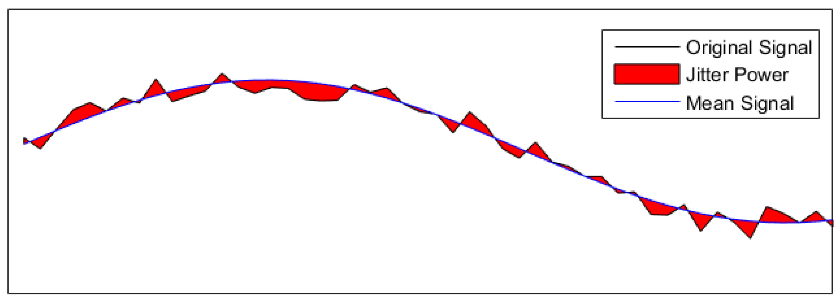
The jitter is a different metric as it tells how well we have modeled the noise of the signal. In a jitter analysis the signal is thought of as a slowly changing signal with a faster noise signal embedded in it.
The slow signal is assumed to be found by taking a low pass filter over the signal to filter out the noise. The jitter analysis measures the power in the jitter from this signal as illustrated in Figure 9.
It the estimated jitter power have been compared with the real jitter power for all the reconstruction methods.
5.3. Non-Intrusive Load Monitoring (NILM) Algorithms
Three popular load disaggregation algorithms have been chosen to disaggregate the meter recovered data. The methods are: FHMM, Parson, and Weiss (more details about these algorithms are in [12]).
These experiments are validated using the F1 score and accuracy metrics. The F1 score is mainly focused on how well the system estimate the ON events. The accuracy measures how many correct guesses there are in relation to the total amount of guesses. The F1 score and the accuracy are calculated based on Equations (14) and (15).
TP is the number of true positives, TN is the number of true negatives, FP is the number of false positives, and FN is the number of false negatives.
From the F1 score’s equation, Figure 10 is built and shown the F1 score of detecting a TV by using Parson and Weiss’s methods combined with gap filling algorithms (i.e., Envelop, Linear, and No gap filling). As shown in Figure 10a, Parson with Linear interpolation gap filling gives good F1 score especially when the error rate is higher than 5%. However, Figure 10b shows that Weiss algorithm with the gap filling algorithms do not give good results.
Based on the previous analysis, we have chosen Linear interpolation gap filling with Parson to reconstruct and disaggregate the SmartHG meter data. The results are stored in the DBCS.
5.4. Outcome Refinement
In Figure 11 is the disaggregation of a TV from house 10 shown for a one day period. The blue line indicate the FHMM algorithms suggestions on when the TV is ON and OFF. The green line is the actual ON and OFF periods, collected from the sub-meters.
As shown in the figure, there is a lot of small spikes that are less than 10 min, and some time is the TV ON for 15 min OFF in 2 and then ON again for another 15 min. This behavior does not fit the normal behavior that is expected from a person. The norm is to see TV more than 20 min at the time, and when a TV is turned OFF it is common that it is turned OFF for at least 15 min before turned ON again. These numbers are a loose estimate, found by observing the sub-meter data.
The values used in the purge and merge process is found experimentally. These parameters gave the best results for the TV’s in the experiments. In a real deployment scenario, where a norm filter was applied, the coefficients must be selected to fit the normal behavior of the residents.
The downside of this approach is that it assumes that the devices are used in a certain manner. For our example of values found for a TV will all watch sessions shorter than 25 min be missed.
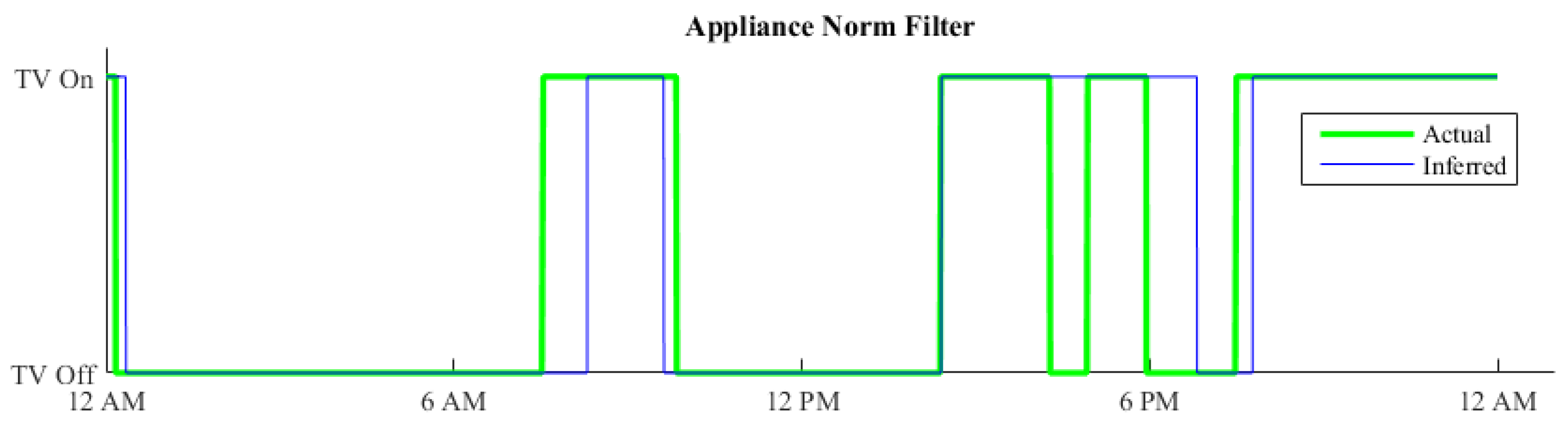
In Figure 12 is the same signal as in Figure 11 filtered by using the norm filter. As seen in Figure 12 does the signal inferred by the filtered FHMM algorithm match more closely to the actual signal.
In this example is the norm knowledge applied as a filter, which can filter the disaggregation result. Another approach could be to integrate the norm knowledge as a component in the state transition probability of the HMM.
Using the specific models, the disaggregation of the main meter signal can be achieved. The statistical disaggregation models selected in this case are found using FHMM algorithm. As discussed in Section 4.4, the disaggregation alone gives a very error-prone signal. The signal is therefore fed through a norm filter. As discussed in Section 4.4, the information about how a user normally would use the appliance can be used to filter the disaggregated data to obtain better results.
The experiment is conducted with four weeks of data been used to train TV specific models for each house. The analysis for the TV station is conducted over a period of six weeks that is not overlapping with the initial four training weeks.
Please notice, the norm filter is only recommended if the accuracy and F1 score of the disaggregation is low. It is undesirable to force the system to make the normal usage as the truth. This can filter away accidental events that lay outside the norm. However, for systems that have a low accuracy and F1 score can this approach help clean the signal.
Results
The viewing habits of the small town obtained by the disaggregation analysis is compared with the actual viewing habit obtained from the sub-meter data. Figure 13 shows the results for the first week. Plots showing the disaggregation of the entire period for each appliance can be found in [49].
The figure shows the viewership, that tells how many in the neighborhood is watching TV at a given time. The green line is the actual viewership, where the blue is the viewership reported by the utility company. The results differed, as one would expect, since the disaggregation process in an environment with high background consumption and high complexity is a hard task. The general trend that many are watching TV in the evening, and not that many in the morning, is represented nicely. This illustrates that the general trend of the viewership is maintained in the disaggregated signal, and this is commonly what is important for this kind of consumer statistics.
In Table 1 is the average number of viewers in 3 h timeslots shown. The shown results in the table are the average of all 6 weeks, split up in the different weekdays.
The results indicates that it is to some degree possible to obtain user information from the disaggregated data. The TV is a relative hard appliance to detect, since there are much different types. The success in this experiment is partly due to the fact that the TV was some of the main consumers of the houses selected, and they had a pure Type-1 behavior
At the current state of NILM is the information only limited to a few devices, since it is hard to detect other appliances than the top consumers in a household. One of the techniques shown to greatly improve the effectiveness of NILM is to switch from the sub 1 Hz sampling range to a higher sampling rate in the kHz range. In the future, there might be smart meters capable of delivering information at high frequency or the NILM techniques have advanced so it is possible to detect all appliances. This will greatly improve the possibility for the service provider to deliver very detailed user behavioral statistics. This information can be of interest for companies developing and selling electronics, since they are able to get accurate user reports about their products.
5.5. NLP and Report Generation
In order to present the outcomes in a user-friendly manner, the stored disaggregated data of individual homes are translated into a natural language report to be presented to the beneficiaries.
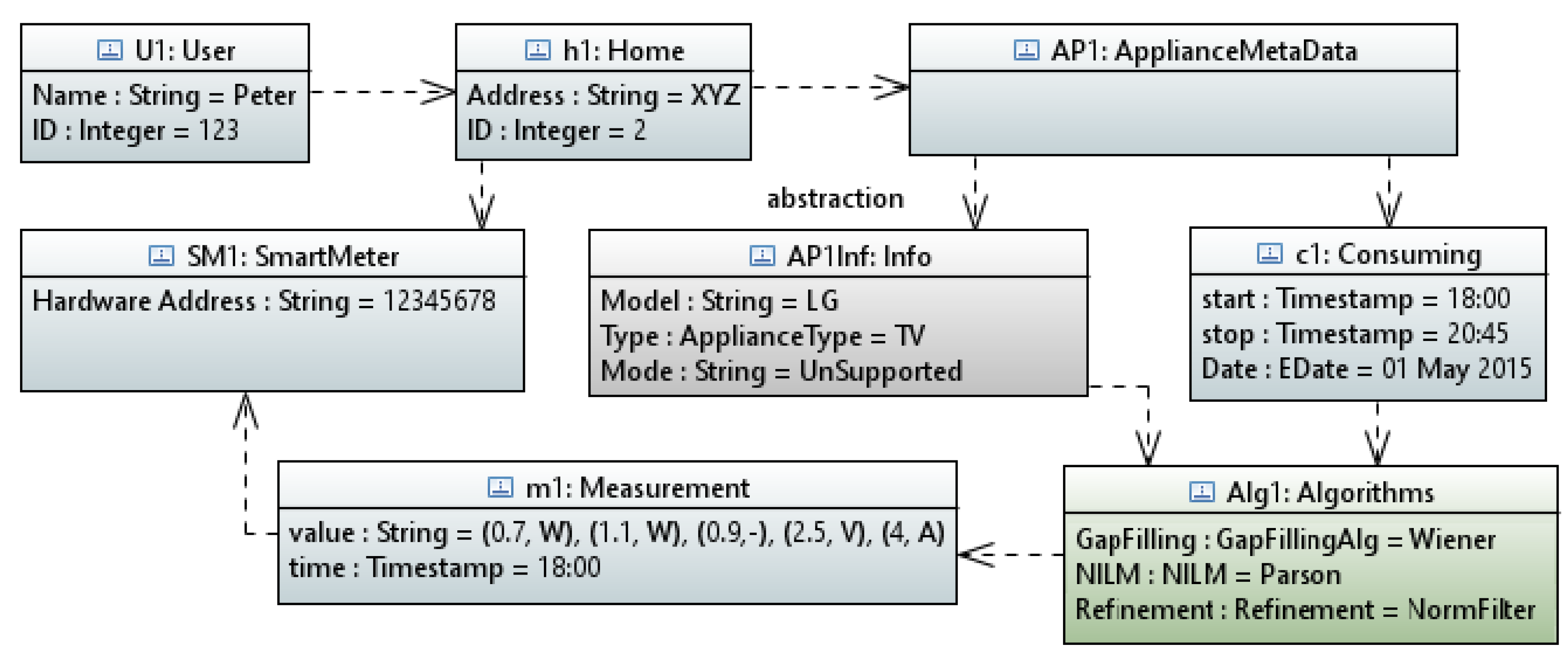
A Python tool has been built to generate an XML description that conforms to the format used by Eclipse Mode-to-Text Language (MTL). The tool uses RESTful interface to gather the data from the DBCS and generates .uml files that can be visualized using Eclipse Plug-in UML editor tool called Papyrus [50]. The tool’s results are shown in Figure 14. The figure shows a UML object diagram that depicts a result of a disaggregated home appliance.
The last step in the natural language synthesis process is to transform the UML object diagram (.uml) into a natural language. This step has been done by developing an Acceleo model-to-text generator to parse and convert the generated UML model into a natural language.The automatically generated natural language report from the parsed UML object diagram (Figure 14):
“Peter (User ID: 123) living in XYZ (Home ID: 2) was watching TV from 18:00 to 20:45 on 1 May 2015”.
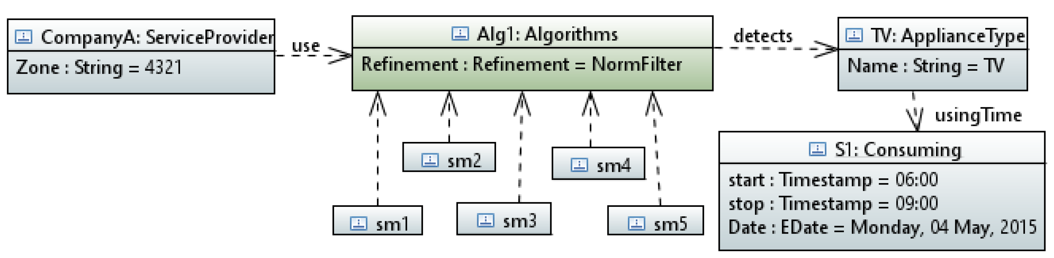
For service providers, the data of a group of users in a certain zone was refined by using norm filter and the outcome is depicted in the object diagram in Figure 15.
The automatically generated natural language report from the parsed UML object diagram in Figure 15:
“CompanyA (Service provider of Zone: 4321) ran algorithm named: Norm Filter on Smart Meters: 1, 2, 3, 4, 5 and detects that the TV was ON from 06:00 to 09:00 on Monday, 4 May 2015”.
The auto-generated reports can be elaborated further based on the amount of information that is required to be presented. For instance, reports can be sent to third-party applications to deliver them to the beneficiaries (e.g., doctors or utility companies).
6. Conclusions
A framework for deducing user behavior from smart meter data has been presented. The framework separates the disaggregation analyses from the natural language data processing. It uses uniform interfaces to exchange data seamlessly between its items. It relies on a shared database which enables easy upgrades of the framework components. Experiments have been performed and the results have been evaluated for choosing the data reconstruction and Load Disaggregation Algorithm (LDA) algorithms. The experiments have shown the complete framework’s data flow process starting from aggregating the main meter data and ending by delivering natural language reports. The framework considers multiple users and combines their behaviors for improving its outcomes. The experiments have validated the feasibility of the framework.
Acknowledgments
The research leading to these results has received funding from the European Union Seventh Framework programme (FP7/2007-2013) under grant agreements no. 619560 (SEMIAH) and no. 317761 (SmartHG).
Author Contributions
Emad Ebeid designed the framwork and built the natural language generator, software interfaces, and wrote the draft of the paper; Rune Heick developed data quality and recovery mechnisms and the machine learning algorithms along with the expermintal results; Rune Hylsberg Jacobsen provided technical suggestions and critically reviewed the paper.
Conflicts of Interest
The authors declare no conflict of interest.
References
- ABI Research. Smart Electricity Meters to Total 780 Million in 2020. Available online: http://abiresearch.com/press/smart-electricity-meters-to-total-780-million-in-2 (accessed on 1 December 2015).
- Green Tech Media. What Will Drive Investment in the Next 60 Million Smart Meters? Available online: greentechmedia.com (accessed on 1 March 2016).
- European Commission. Benchmarking Smart Metering Deployment in the EU-27 with a Focus on Electricity. Available online: http://eur-lex.europa.eu/ (accessed on 1 June 2014).
- Depuru, S.; Wang, L.; Devabhaktuni, V. Smart Meters for Power Grid: Challenges, Issues, Advantages and Status. Renew. Sustain. Energy Rev. 2011, 15, 2736–2742. [Google Scholar] [CrossRef]
- Mancini, T.; Mari, F.; Melatti, I.; Salvo, I.; Tronci, E.; Gruber, J.K.; Hayes, B.; Prodanovic, M.; Elmegaard, L. User Flexibility Aware Price Policy Synthesis for Smart Grids. In Proceedings of the 2015 Euromicro Conference on Digital System Design, Funchal, Portugal, 26–28 August 2015; pp. 478–485. [Google Scholar]
- Jacobsen, R.; Tørring, N.; Danielsen, B.; Hansen, M.; Pedersen, E. Towards an App Platform for Data Concentrators. In Proceedings of the IEEE ISGT Innovative Smart Grid Technologies Conference (ISGT), Washington, DC, USA, 19–22 February 2014; pp. 1–5. [Google Scholar]
- Trung, K.N.; Zammit, O.; Dekneuvel, E.; Nicolle, B.; Nguyen Van, C.; Jacquemod, G. An Innovative Non-Intrusive Load Monitoring System for Commercial and Industrial Application. In Proceedings of the International Conference on Advanced Technologies for Communications, Hanoi, Vietnam, 10–12 October 2012; pp. 23–27. [Google Scholar]
- Wang, K.; Wang, Y.; Hu, X.; Sun, Y.; Deng, D.J.; Vinel, A.; Zhang, Y. Wireless Big Data Computing in Smart Grid. IEEE Wirel. Commun. 2017, 24, 58–64. [Google Scholar] [CrossRef]
- Dinesh, H.G.C.P.; Perera, P.H.; Godaliyadda, G.M.R.I.; Ekanayake, M.P.B.; Ekanayake, J.B. Residential Appliance Monitoring Based on Low Frequency Smart Meter Measurements. In Proceedings of the 2015 IEEE International Conference on Smart Grid Communications (SmartGridComm), Miami, FL, USA, 2–5 November 2015; pp. 878–884. [Google Scholar]
- Mikkelsen, S.A.; Jacobsen, R.H.; Terkelsen, A.F. DB&A: An Open Source Web Service for Meter Data Management. In Proceedings of the Symposium on Service-Oriented System Engineering, Oxford, UK, 29 March–2 April 2016. [Google Scholar]
- Batra, N.; Kelly, J.; Parson, O.; Dutta, H.; Knottenbelt, W.; Rogers, A.; Singh, A.; Srivastava, M. NILMTK: An Open Source Toolkit for Non-intrusive Load Monitoring. In Proceedings of the 5th International Conference on Future Energy Systems, Cambridge, UK, 1–13 June 2014. [Google Scholar]
- Beckel, C.; Kleiminger, W.; Cicchetti, R.; Staake, T.; Santini, S. The ECO Data Set and the Performance of Non-Intrusive Load Monitoring Algorithms. In Proceedings of the 1st ACM Conference on Embedded Systems for Energy-Efficient Buildings, Memphis, TN, USA, 3–6 November 2014; pp. 80–89. [Google Scholar]
- Ruzzelli, A.G.; Nicolas, C.; Schoofs, A.; O’Hare, G.M.P. Real-Time Recognition and Profiling of Appliances through a Single Electricity Sensor. In Proceedings of the 7th Annual IEEE Communications Society Conference on Sensor, Mesh and Ad Hoc Communications and Networks (SECON), Boston, MA, USA, 21–25 June 2010; pp. 1–9. [Google Scholar]
- Liao, J.; Elafoudi, G.; Stankovic, L.; Stankovic, V. Non-intrusive appliance load monitoring using low-resolution smart meter data. In Proceedings of the 2014 IEEE International Conference on Smart Grid Communications (SmartGridComm), Venice, Italy, 3–6 November 2014; pp. 535–540. [Google Scholar]
- Chiang, J.; Zhang, T.; Chen, B.; Hu, Y.C. Load disaggregation using harmonic analysis and regularized optimization. In Proceedings of the Asia-Pacific Signal Information Processing Association Annual Summit and Conference (APSIPA ASC), Hollywood, CA, USA, 3–6 December 2012; pp. 1–4. [Google Scholar]
- International Organization for Standardization. ISO19157 Geographic Information & Data Quality; International Organization for Standardization: Geneva, Switzerland, 2013. [Google Scholar]
- Pastorello, G.; Agarwal, D.; Papale, D.; Samak, T.; Trotta, C.; Ribeca, A.; Poindexter, C.; Faybishenko, B.; Gunter, D.; Hollowgrass, R.; et al. Observational Data Patterns for Time Series Data Quality Assessment. In Proceedings of the 2014 IEEE 10th International Conference on e-Science ( e-Science ’14), Sao Paulo, Brazil, 20–24 October 2014; IEEE Computer Society: Washington, DC, USA, 2014; Volume 1, pp. 271–278. [Google Scholar]
- Moghtaderi, A.; Borgnat, P.; Flandrin, P. Gap-Filling by the empirical mode decomposition. In Proceedings of the 2012 IEEE International Conference on Acoustics, Speech and Signal Processing (ICASSP), Kyoto, Japan, 25–30 March 2012; pp. 3821–3824. [Google Scholar]
- Manolakis, D.; Ingle, V. Applied Digital Signal Processing: Theory and Practice; Cambridge University Press: New York, NY, USA, 2011. [Google Scholar]
- Meng, H.; Guan, Y.L.; Chen, S. Modeling and analysis of noise effects on broadband power-line communications. IEEE Trans. Power Deliv. 2005, 20, 630–637. [Google Scholar] [CrossRef]
- Warren, G.H. Power Line Filter for Transient and Continuous Noise Suppression. U.S. Patent 4,698,721, 6 October 1987. [Google Scholar]
- Meijer, M.; Vullings, L.; Bulens, J.; Rip, F.; Boss, M.; Hazeu, G.; Storm, M. Spatial Data Quality and a Workflow Tool. Int. Arch. Photogramm. Remote Sens. Spat. Inf. Sci. 2015, 40. [Google Scholar] [CrossRef]
- Simader, A.M.; Kluger, B.; Neumann, N.K.N.; Bueschl, C.; Lemmens, M.; Lirk, G.; Krska, R.; Schuhmacher, R. QCScreen: A software tool for data quality control in LC-HRMS based metabolomics. BMC Bioinform. 2015, 16. [Google Scholar] [CrossRef] [PubMed]
- Jacobsen, R.; Mikkelsen, S.A. Infrastructure for Intelligent Automation Services in the Smart Grid. Wirel. Pers. Commun. 2014, 76, 125–147. [Google Scholar] [CrossRef]
- Burden, H.; Heldal, R. Natural Language Generation from Class Diagrams. In Proceedings of the 8th International Workshop on Model-Driven Engineering, Verification and Validation, Wellington, New Zealand, 17 October 2011; ACM: New York, NY, USA, 2011. [Google Scholar]
- International Organization for Standardization. ISO 8402:1994 Quality Management and Quality Assurance—Vocabulary; International Organization for Standardization: Geneva, Switzerland, 1994. [Google Scholar]
- Witten, I.H.; Frank, E. Data Mining: Practical Machine Learning Tools and Techniques; Morgan Kaufmann: San Francisco, CA, USA, 2005. [Google Scholar]
- Object Management Group. Unified Modeling Language, (Version 2.5); Object Management Group: Needham, MA, USA, 2013; Available online: http://uml.org (accessed on 15 March 2017).
- Eclipse. Acceleo. Available online: http://eclipse.org/acceleo/ (accessed on 15 March 2016).
- Ebeid, E.; Rotger-Griful, S.; Mikkelsen, S.A.; Jacobsen, R.H. A Methodology to Evaluate Demand Response Communication Protocols for the Smart Grid. In Proceedings of the 2015 IEEE International Conference on Communication Workshop (ICCW), London, UK, 8–12 June 2015; pp. 2012–2017. [Google Scholar]
- ZigBee Alliance. ZigBee. Available online: www.zigbee.org (accessed on 1 December 2016).
- Ferreira, P.J.S.G. Interpolation and the discrete Papoulis-Gerchberg algorithm. IEEE Trans. Signal Process. 1994, 42, 2596–2606. [Google Scholar] [CrossRef]
- Marques, M.; Neves, A.; Marques, J.S.; Sanches, J. The Papoulis-Gerchberg Algorithm with Unknown Signal Bandwidth. In Proceedings of the Third International Conference on Image Analysis and Recognition (ICIAR 2006) Part I, Póvoa de Varzim, Portugal, 18–20 September 2006; Campilho, A., Kamel, M.S., Eds.; Springer: Berlin/Heidelberg, Germany, 2006; pp. 436–445. [Google Scholar]
- Rune Heick. P-G Algorithm. Available online: https://github.com/RuneHeick/SpecialeAppendix/tree/master/P-G%20Algo (accessed on 1 April 2016).
- Thomson, D.; Lanzerotti, L.; Maclennan, C. Interplanetary magnetic field: Statistical properties and discrete modes. J. Geophys. Res. Space Phys. 2001, 106, 15941–15962. [Google Scholar] [CrossRef]
- Rune Heick. Weiner Gap Filter Algorithm. Available online: https://github.com/RuneHeick/SpecialeAppendix/tree/\master/SSA%20Algo (accessed on 15 March 2016).
- Kondrashov, D.; Ghil, M. Spatio-temporal filling of missing points in geophysical data sets. Nonlinear Process. Geophys. 2006, 13, 151–159. [Google Scholar] [CrossRef]
- Rune Heick. Spatio-Temporal Filling Algorithm. Available online: https://github.com/RuneHeick/SpecialeAppendix/tree/\master/SSA%20Algo (accessed on 15 March 2016).
- Rune Heick. Envelope Filling Algorithm. Available online: https://github.com/RuneHeick/SpecialeAppendix/tree/master/\Env%20Algo (accessed on 15 March 2016).
- Rune Heick. Empirical Mode Decomposition Filling Algorithm. Available online: https://github.com/RuneHeick/SpecialeAppendix/tree/master/Emd%20Algo (accessed on 15 March 2016).
- Bonino, D.; Corno, F.; Russis, L.D. Home energy consumption feedback: A user survey. Energy Build. 2012, 47, 383–393. [Google Scholar] [CrossRef]
- Zoha, A.; Gluhak, A.; Imran, M.A.; Rajasegarar, S. Non-Intrusive Load Monitoring Approaches for Disaggregated Energy Sensing: A Survey. Sensors 2012, 12, 16838–16866. [Google Scholar] [CrossRef] [PubMed]
- Srinivasan, D.; Ng, W.S.; Liew, A.C. Neural-network-based signature recognition for harmonic source identification. IEEE Trans. Power Deliv. 2006, 21, 398–405. [Google Scholar] [CrossRef]
- Patel, S.N.; Robertson, T.; Kientz, J.A.; Reynolds, M.S.; Abowd, G.D. At the Flick of a Switch: Detecting and Classifying Unique Electrical Events on the Residential Power Line (Nominated for the Best Paper Award). In Proceedings of the 9th International Conference on Ubiquitous Computing (UbiComp 2007), Innsbruck, Austria, 16–19 September 2007; Krumm, J., Abowd, G.D., Seneviratne, A., Strang, T., Eds.; Springer: Berlin/Heidelberg, Germany, 2007; pp. 271–288. [Google Scholar]
- Ghahramani, Z.; Jordan, M.I. Factorial Hidden Markov Models. Mach. Learn. 1997, 29, 245–273. [Google Scholar] [CrossRef]
- Kolter, J.Z.; Jaakkola, T. Approximate Inference in Additive Factorial HMMs with Application to Energy Disaggregation. In Proceedings of the Fifteenth International Conference on Artificial Intelligence and Statistics (AISTATS-12), La Palma, Canary Islands, Spain, 21–23 April 2012. [Google Scholar]
- Weiss, M.; Helfenstein, A.; Mattern, F.; Staake, T. Leveraging smart meter data to recognize home appliances. In Proceedings of the 2012 IEEE International Conference on Pervasive Computing and Communications (PerCom), Lugano, Switzerland, 19–23 March 2012; pp. 190–197. [Google Scholar]
- Parson, O.; Ghosh, S.; Weal, M.; Rogers, A. Non-intrusive load monitoring using prior models of general appliance types. In Proceedings of the Twenty-Sixth AAAI Conference on Artificial Intelligence, Toronto, ON, Canada, 22–26 July 2012; pp. 356–362. [Google Scholar]
- Rune Heick. Detailed results from the disaggregation of TV’s in Case study. Available online: https://github.com/RuneHeick/SpecialeAppendix/tree/master/Case%20Study%20Plot (accessed on 15 March 2016).
- Eclipse. Papyrus. Available online: https://eclipse.org/papyrus/ (accessed on 30 December 2016).
Figure 1.
Conceptual view of the proposed framework.
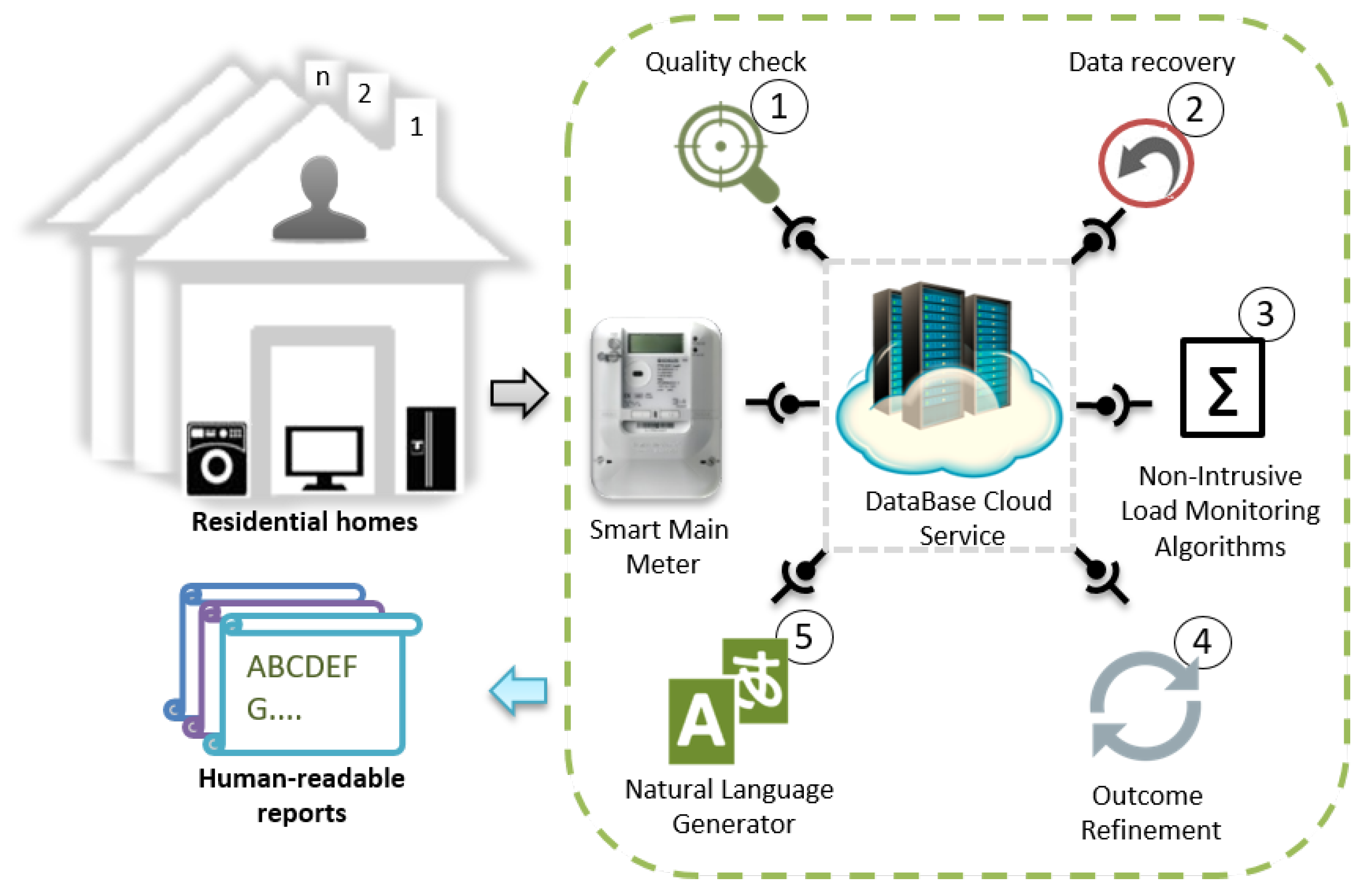
Figure 2.
Framework structure.

Figure 3.
Illustration of availability analysis.

Figure 4.
The disaggregation process.
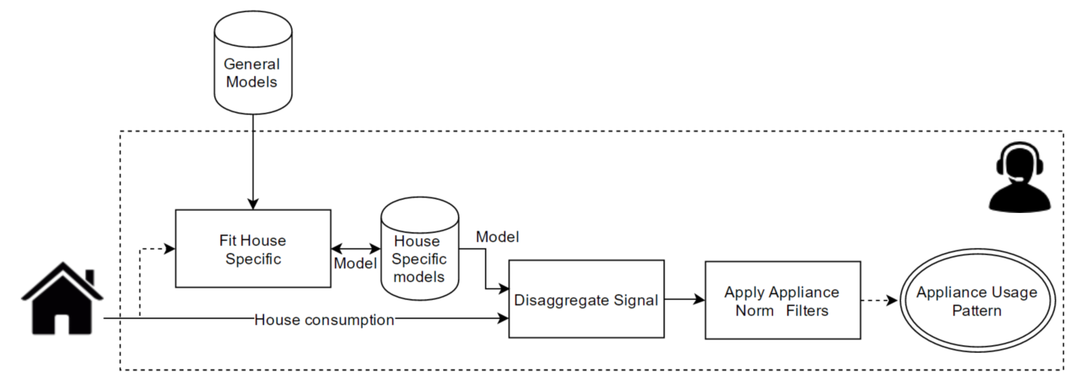
Figure 5.
UML class diagram of the framework architecture.
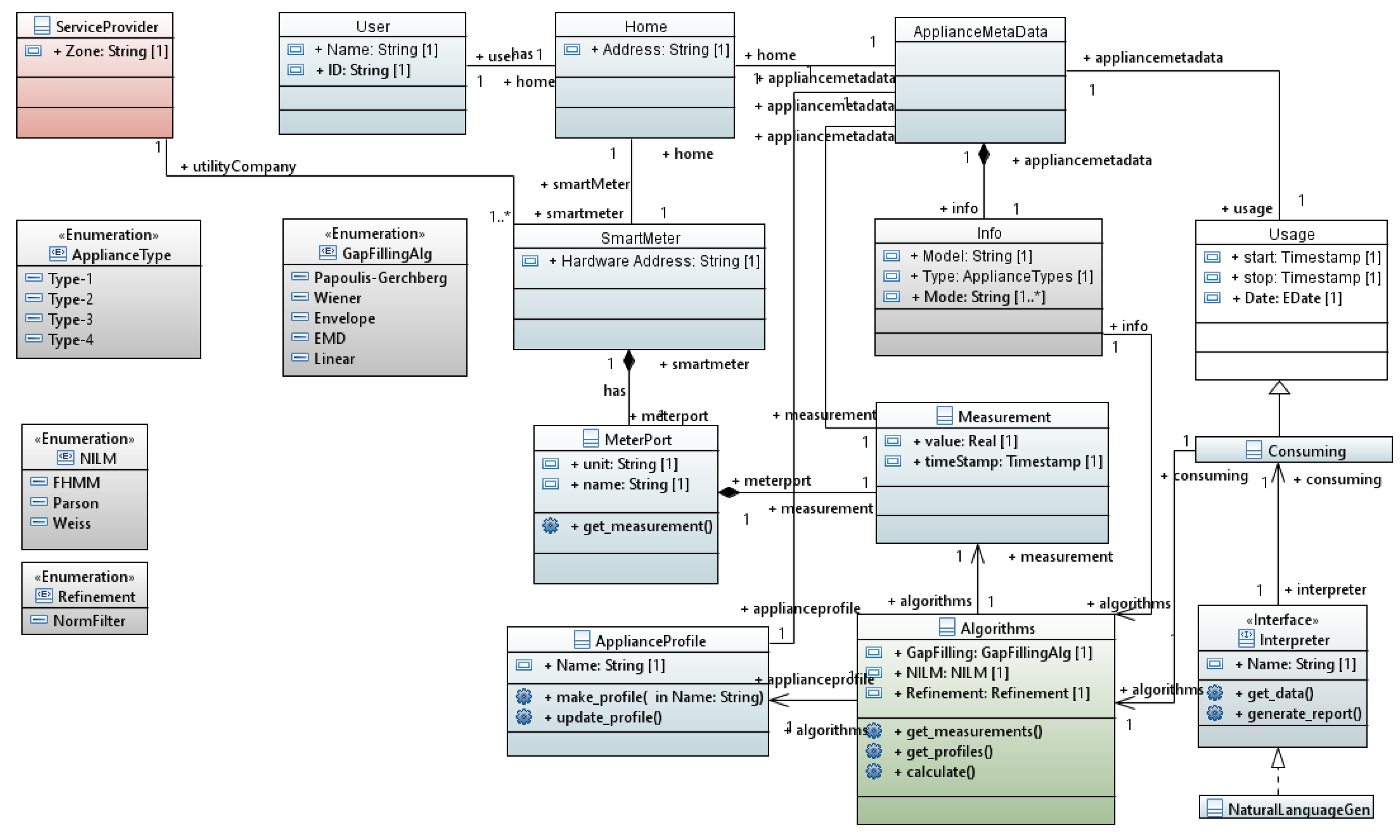
Figure 6.
Data quality of 25 houses in the SmartHG project.
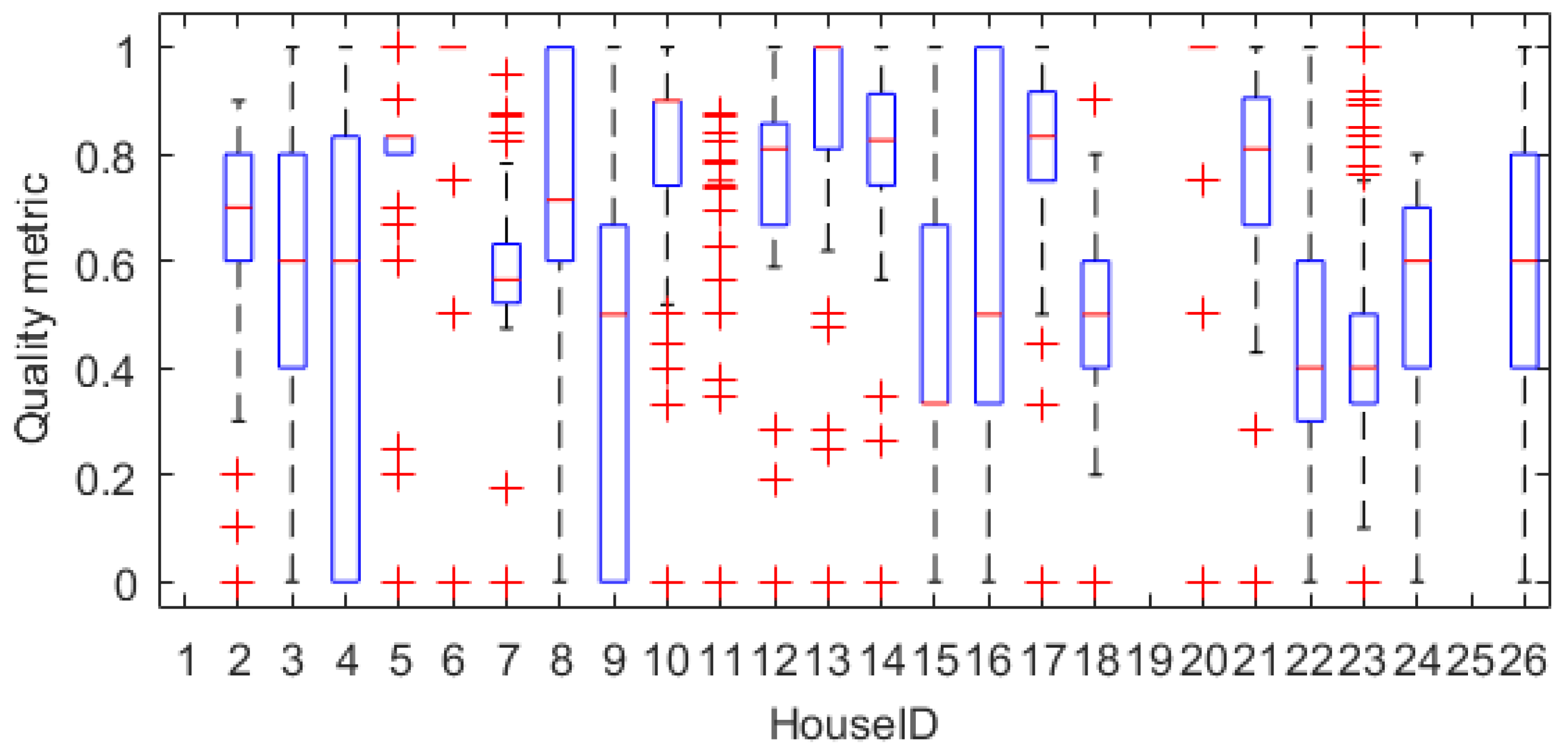
Figure 7.
Stochastic effect on prediction.
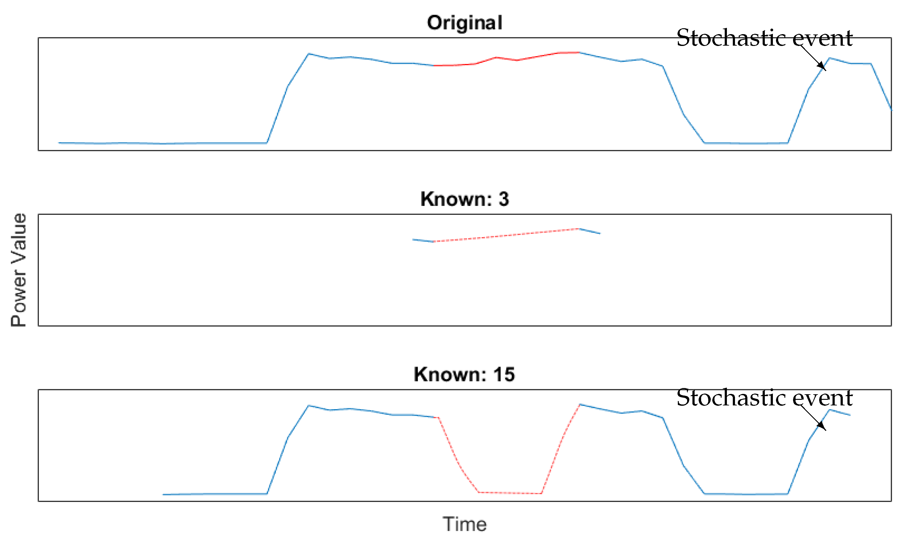
Figure 8.
Frequency comparison of the reconstruction methods.
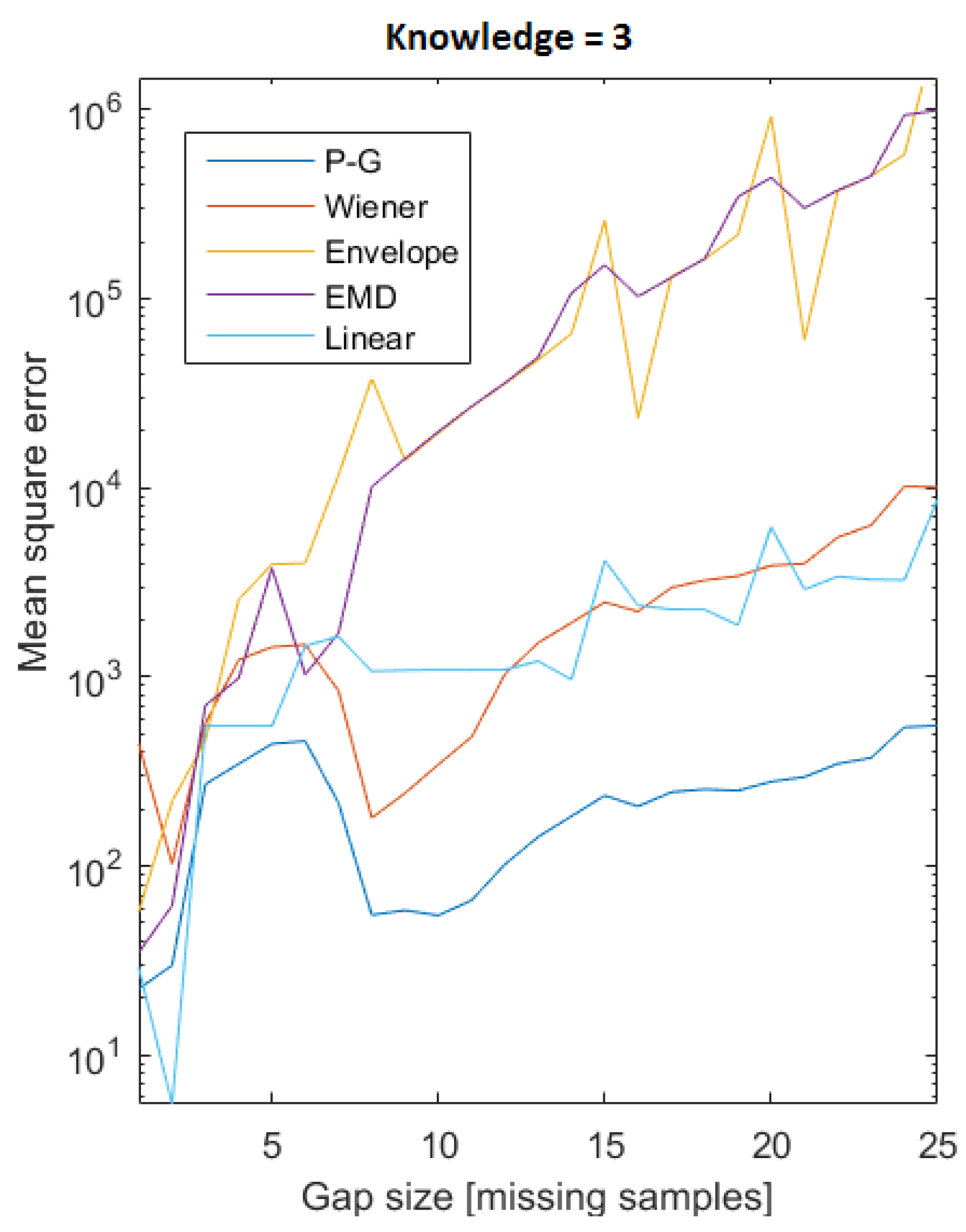
Figure 9.
Jitter power illustration.

Figure 10.
F1 score of the load disaggregation methods.
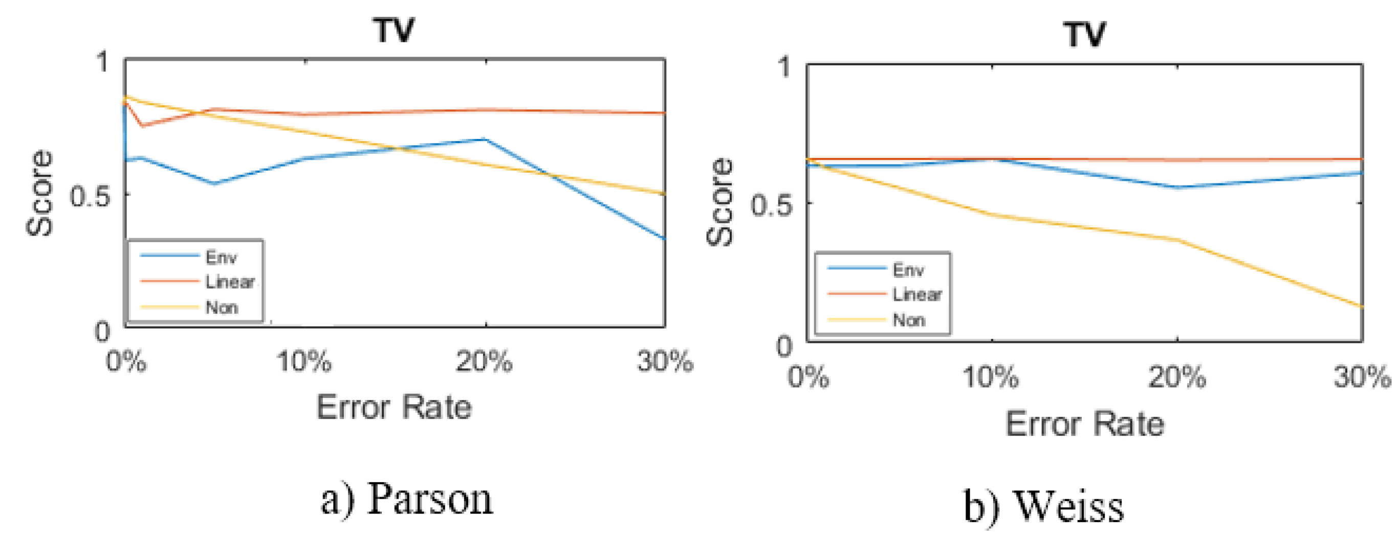
Figure 11.
Disaggregation of TV 1 from house 10.
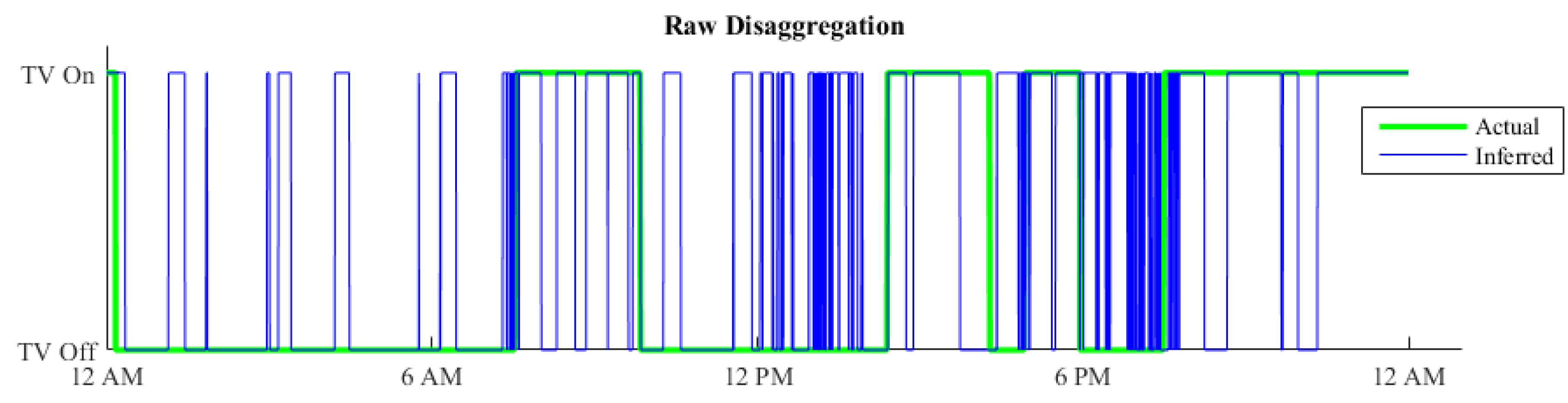
Figure 12.
Purged and merged signal from a TV.

Figure 13.
Viewership in week one.
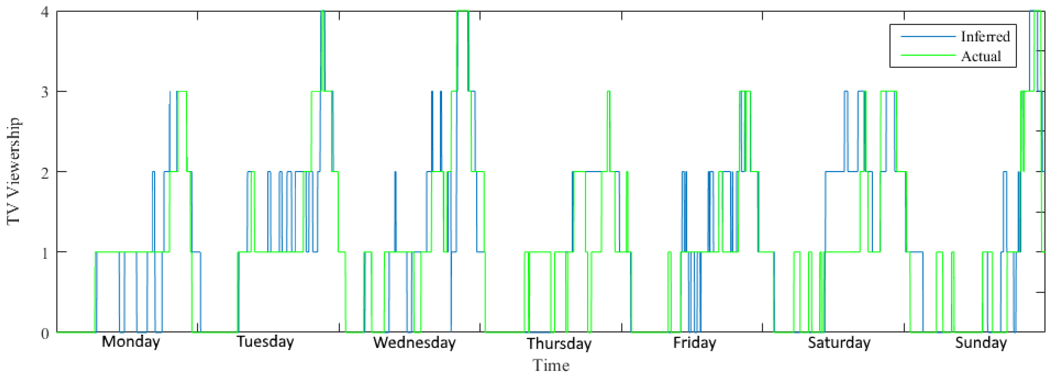
Figure 14.
UML object diagram of a home.

Figure 15.
UML object diagram of a group of homes.

Table 1.
Average viewership in a 6 weeks period.
| Time of Day | |||||||||
|---|---|---|---|---|---|---|---|---|---|
| 00–03 | 03–06 | 06–09 | 09–12 | 12–13 | 15–18 | 18–21 | 21–00 | ||
| Monday | Inferred | 0.12 | 0.00 | 0.66 | 1.19 | 1.02 | 1.31 | 2.39 | 2.08 |
| True | 0.13 | 0.28 | 0.98 | 0.87 | 0.68 | 1.28 | 2.49 | 1.72 | |
| Tuesday | Inferred | 0.13 | 0.28 | 0.98 | 0.87 | 0.68 | 1.28 | 2.49 | 1.72 |
| True | 0.19 | 0.09 | 0.39 | 0.88 | 0.73 | 1.24 | 2.23 | 2.26 | |
| Wednesday | Inferred | 0.19 | 0.09 | 0.39 | 0.88 | 0.73 | 1.24 | 2.23 | 2.26 |
| True | 0.09 | 0.30 | 0.58 | 0.79 | 0.77 | 1.42 | 2.72 | 2.11 | |
| Thursday | Inferred | 0.09 | 0.30 | 0.58 | 0.79 | 0.77 | 1.42 | 2.72 | 2.11 |
| True | 0.12 | 0.09 | 0.31 | 0.96 | 1.12 | 1.69 | 2.86 | 2.30 | |
| Friday | Inferred | 0.12 | 0.09 | 0.31 | 0.96 | 1.12 | 1.69 | 2.86 | 2.30 |
| True | 0.10 | 0.18 | 0.66 | 0.91 | 0.74 | 1.65 | 3.17 | 2.35 | |
| Saturday | Inferred | 0.10 | 0.18 | 0.66 | 0.91 | 0.74 | 1.65 | 3.17 | 2.35 |
| True | 0.28 | 0.17 | 0.95 | 0.77 | 1.39 | 1.36 | 2.26 | 2.10 | |
| Sunday | Inferred | 0.28 | 0.17 | 0.95 | 0.77 | 1.39 | 1.36 | 2.26 | 2.10 |
| True | 0.12 | 0.00 | 1.01 | 0.96 | 0.96 | 1.33 | 1.93 | 1.65 | |
© 2017 by the authors. Licensee MDPI, Basel, Switzerland. This article is an open access article distributed under the terms and conditions of the Creative Commons Attribution (CC BY) license (http://creativecommons.org/licenses/by/4.0/).
Share and Cite
MDPI and ACS Style
Ebeid, E.; Heick, R.; Jacobsen, R.H. Deducing Energy Consumer Behavior from Smart Meter Data. Future Internet 2017, 9, 29. https://doi.org/10.3390/fi9030029
AMA Style
Ebeid E, Heick R, Jacobsen RH. Deducing Energy Consumer Behavior from Smart Meter Data. Future Internet. 2017; 9(3):29. https://doi.org/10.3390/fi9030029
Chicago/Turabian StyleEbeid, Emad, Rune Heick, and Rune Hylsberg Jacobsen. 2017. "Deducing Energy Consumer Behavior from Smart Meter Data" Future Internet 9, no. 3: 29. https://doi.org/10.3390/fi9030029
Note that from the first issue of 2016, this journal uses article numbers instead of page numbers. See further details here.