Cost-Aware IoT Extension of DISSECT-CF


1
Software Engineering Department, University of Szeged, 6720 Szeged, Hungary
2
Department of Computer Science, Liverpool John Moores University, Liverpool L3 3AF, UK
*
Authors to whom correspondence should be addressed.
Future Internet 2017, 9(3), 47; https://doi.org/10.3390/fi9030047
Submission received: 18 July 2017
/
Revised: 31 July 2017
/
Accepted: 10 August 2017
/
Published: 14 August 2017
(This article belongs to the Special Issue Big Data and Internet of Thing)
Abstract
:In the age of the Internet of Things (IoT), more and more sensors, actuators and smart devices get connected to the network. Application providers often combine this connectivity with novel scenarios involving cloud computing. Before implementing changes in these large-scale systems, an in-depth analysis is often required to identify governance models, bottleneck situations, costs and unexpected behaviours. Distributed systems simulators help in such analysis, but they are often problematic to apply in this newly emerging domain. For example, most simulators are either too detailed (e.g., need extensive knowledge on networking), or not extensible enough to support the new scenarios. To overcome these issues, we discuss our IoT cost analysis oriented extension of DIScrete event baSed Energy Consumption simulaTor for Clouds and Federations (DISSECT-CF). Thus, we present an in-depth analysis of IoT and cloud related pricing models of the most widely used commercial providers. Then, we show how the fundamental properties (e.g., data production frequency) of IoT entities could be linked to the identified pricing models. To allow the adoption of unforeseen scenarios and pricing schemes, we present a declarative modelling language to describe these links. Finally, we validate our extensions by analysing the effects of various identified pricing models through five scenarios coming from the field of weather forecasting.
1. Introduction
Internet of Things (IoT) is a rapidly emerging concept where sensors, actuators and smart devices are often connected to cloud systems. Clouds are used in scenarios in which data from a large set of sensors is processed and often fed back to actuators or smart devices. As the number of devices with connected sensors and actuators are reaching new heights every day, the way they are integrated to the cloud computing ecosystem is also rapidly changing. As a result, IoT systems integrators often need new experimental techniques—e.g., simulators—which allow them to understand the behaviour of systems of previously unprecedented scale.
Recently, a wide range of IoT oriented simulators have risen [1,2,3]. Regrettably, these are use case limited (e.g., they only focus on big data processing). In addition, they are often focused on very specific sensors or sensor behaviour, neglecting the financial side of operating large scale IoT systems. Finally, these simulators are rarely scaling to match the number of devices foreseen in IoT systems of tomorrow.
In this paper, we lay the foundations for flexible and scalable modelling of IoT systems and their related cost models through our extensions to the simulator: DIScrete event baSed Energy Consumption simulaTor for Clouds and Federations (DISSECT-CF) [4]. The main contributions of this paper are: (i) the analysis of operating costs of IoT scenarios by introducing a model of provider pricing schemes, (ii) the comparison of usage costs of a real world meteorological application at four providers, (iii) the extension of a state-of-the-art simulator for modelling IoT sensors and applying provider pricing models on them, and finally (iv) the evaluation of the considered meteorological case study in the simulator. Although scaling the simulation over several nodes is a relevant topic to meet the demands of the newest IoT scenarios, this topic is out of scope here as it was discussed before by [5]. Similarly, detailed information on sensor produced data (e.g., how accurate it is) and algorithmic reactions to the data are out of scope of this paper, as these would require such level of detail that it would hinder our objective to support large scale IoT-Cloud systems.
One of the earliest use of connected sensors is from the field of weather forecasting. The findings of the paper are evaluated through five weather forecasting scenarios: we used the public data available on the sensors operated by the crowdsourced meteorological service of Hungary called Idokep.hu [6]. Using the extended DISSECT-CF, we set up an extensive network of simulated sensors (with over 400 devices encompassing over 3000 individual sensors) and evaluated data collection and analysis techniques, as if they would be executed in a state-of-the-art infrastructure as a service system.
The structure of the paper is the following. First, in Section 2, we continue with the discussion of the state of the art. Next, in Section 3, we discuss the extensions applied to the DISSECT-CF simulator. Later, Section 4 discusses our weather forecasting case study and evaluates our extensions with real-life scenarios. Finally, Section 5 concludes our work.
2. Related Work
There are many simulators available to examine distributed and specifically cloud systems. Nevertheless, there are some more specific IoT simulators closer to our approach. Han et al. [2] have designed the Devices Profile for Web Services Simulation Toolkit (DPWSim), which is a simulation toolkit to support the development of service-oriented and event-driven IoT applications with secure web service capabilities. Its aim is to support the OASIS (Organization for the Advancement of Structured Information Standards) standard Devices Profile for Web Services. SimIoT [1] is derived from the SimIC simulation framework [7]. It introduces several techniques to simulate the communication between an IoT sensor and the cloud, but it is limited to compute activity modelling.
Moschakis and Karatza [8] introduce several simulation concepts for IoT systems. First, they show how the interfacing between the various cloud providers and IoT systems could be modelled (even including workload models) in a simulation. Unfortunately, they mainly discuss the behaviour of cloud systems that support the processing of data originated from the IoT system. Silva et al. [9] deal with the dynamic nature of IoT systems, they investigate fault behaviours and introduce a fault model for such systems. Although faults are important, the scalability of the introduced fault behaviours and concepts are insufficient for large scale systems.
Khan et al. [10] introduce a novel infrastructure coordination technique that supports the use of larger scale IoT systems. They build on CloudSim [11] and provide customizations that are tailored for their specific home automation scenarios and therefore limit the applicability of their extensions. Zeng et al. [3] proposed IOTSim that supports and enables simulation of big data processing in IoT systems limiting themselves to the MapReduce model. They also presented a real case study that validates the effectiveness of their simulator.
In the field of resource abstraction for IoT, efforts aimed at the description and implementation of languages and frameworks for efficient representation, annotation and processing of sensed data. The integration of IoT and clouds has been envisioned by Botta et al. [12] and by Nastic et al. [13]. They argue that system designers and operations managers face numerous challenges to realize IoT cloud systems in practice, due to the complexity and diversity of their requirements in terms of IoT resources consumption, customization and runtime governance as well as context awareness [14]. We build on these results and target our contribution in the field of cost modelling in IoT Cloud simulations.
3. Cost Modeling in DISSECT-CF
We aim at supporting the simulation of thousands (or more) devices participating in previously unforeseen/existing IoT scenarios that have not been examined before in more detail (e.g., in terms of scalability, energy efficiency or management costs). As this aim requires a high performance resource sharing mechanism, we have chosen to extend the DISSECT-CF [4] simulator because of its unified resource sharing foundation.
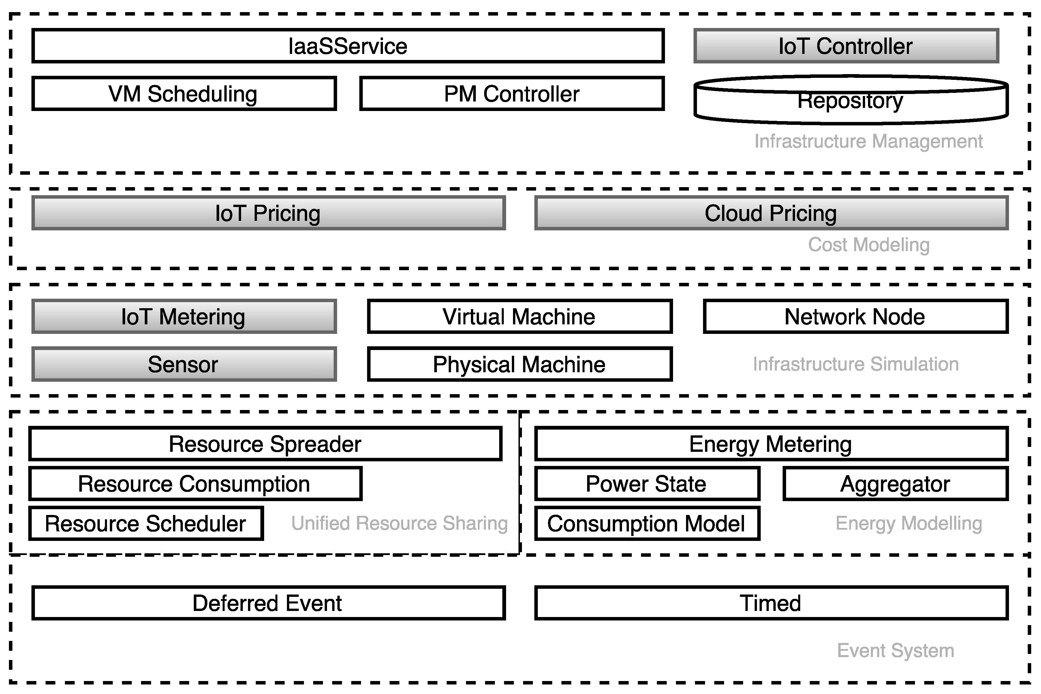
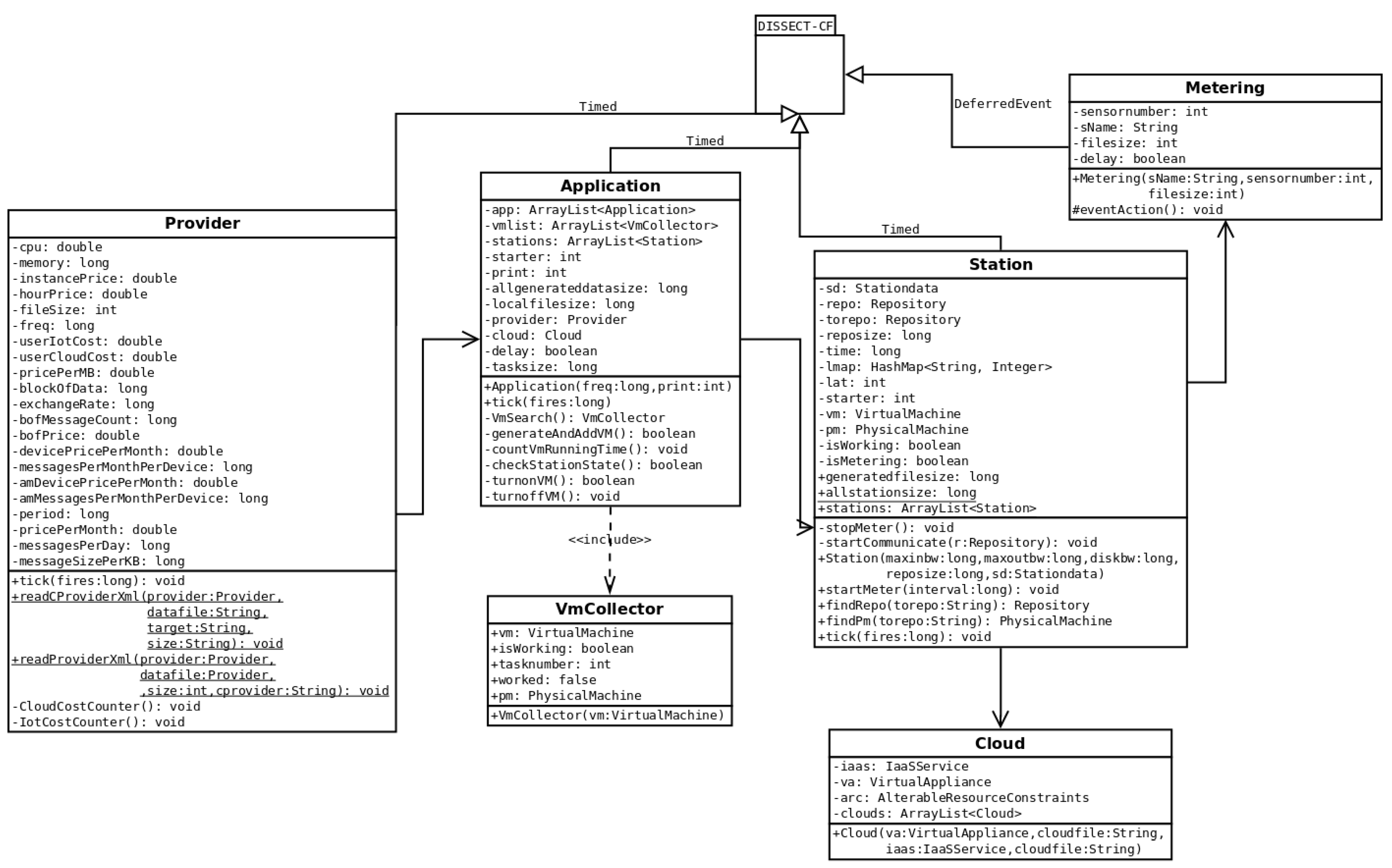
DISSECT-CF is a compact open source simulator [15] focusing on the internals of IaaS (Infrastructure as a Service) systems. Figure 1 presents its architecture including our extensions (denoted with grey colour). There are six subsystems (encircled with dashed lines) implemented, each responsible for a particular functionality: (i) event system—the primary time reference; (ii) unified resource sharing—models low-level resource bottlenecks; (iii) energy modelling—for the analysis of energy-usage patterns of resources (e.g., CPUs) or their aggregations; (iv) infrastructure simulation—for physical/virtual machines, sensors and networking; (v) cost modelling—for managing IoT and cloud provider pricing schemes, and (vi) infrastructure management—provides a cloud like API (Application Programming Interface), cloud level scheduling, and IoT system monitoring and management.
Our current extension performed within this work focuses on IoT and cost management. We introduced the following new components to model IoT systems: Sensor, IoT Metering and IoT Controller. Sensors are essential parts of IoT systems, and usually they are passive entities (actuators could change their surrounding environment though). Their performance is limited by their network gateway’s (i.e., the device which polls for the measurements and sends them away) connectivity and maximum update frequency. Our network gateway model builds on DISSECT-CF’s already existing Network Node model which allows changes in connection quality as well. Our model of the Sensor component is used to define the sensor type, properties and connections to a cloud system. IoT Metering is used to define and characterize messages coming from sensors, and the IoT Controller is used for sensor creation and management.
To incorporate cost management, we enabled defining and applying provider pricing schemes both for IoT and cloud part of the simulated environments. These schemes are managed by the IoT and Cloud Pricing components of the Cost modeling subsystem of DISSECT-CF, as shown in Figure 1.
3.1. IoT Pricing
In our simulation model, we aim to investigate certain IoT cloud applications; therefore, we need to define and monitor the following parameters: the number of sensors or devices used, the total number of messages (and their data) sent in a certain period of time, and the uptime and capacity of virtual machines used to provide ingest services. Based on these parameters, we can estimate how our application would be charged after operating its system for a certain amount of time at a concrete IoT cloud provider.
The calculation of the prices depends on different methods. Some providers bill only according to the number of messages sent, while others also charge for the number of devices used. The situation is very similar if we consider the virtual machine rental or application service prices. One can be charged after GB-hour (GigaByte-hour or uptime) or according to a fix monthly service price. This price also depends on the configuration of the virtual machine or the selected application service, especially the mount of RAM used or the number of CPU cores or their clock signal.
We considered the following, most popular providers as the base of our extension: (i) Microsoft and its IoT platform called Azure IoT Hub [16], (ii) IBM’s Bluemix IoT platform [17], the services of (iii) Amazon (AWS IoT) [18], and (iv) Oracle’s IoT platform [19]. We took into account the prices publicly available on the websites of the providers and if it necessary we asked for clarifications via email.
3.1.1. Azure IoT Hub
Concerning the IoT side pricing, Azure IoT Hub charges one after the chosen edition/tier. This means that there are intervals for the number of messages used in a month. Azure also comes with some additional platform services when similarly to other providers, but we only kept the general parts to allow the identification of common pricing components. There is a restriction for message sizes that depends on the chosen tiers. One can choose from four tiers, Free, S1, S2, S3. Each of them vary in price and the total messages allowed per day. Message and group size of the Free tier is significantly more limited compared to the other tiers.
3.1.2. IBM Bluemix
IBM Bluemix IoT platform’s pricing follows the “pay as you go” approach. Bluemix only charges after the MiB of data exchanged. They differentiate three categories in terms of data usage and each of them comes with a different price per MiB. The more we transfer the less our price will be per MiB.
3.1.3. Amazon’s IoT platform
Amazon’s IoT platform can also be classified as a “pay as you go” service. Prices have two components: publishing cost (the number of messages published to AWS IoT) and delivery cost (the number of messages delivered by AWS IoT to devices or applications). A message is a 512-byte block of data and the pricing in EU and US regions denotes 5 US dollars per million messages. In addition, there is no charge for deliveries to some other AWS Services.
3.1.4. Oracle’s IoT Platform
Finally, we investigated pricing of the Oracle’s IoT solution. This pricing method is slightly different from the three providers described before. It is more similar to Azure’s tiers than to the completely “pay as you go” billing like in Bluemix. The information was gathered from and we calculated with the so-called Metered Services. There are four product categories regarding the used devices (wearable, consumer, telematics and business). Categories determine the monthly device price and the number of messages that can be sent by that particular type of device. In addition, there is a restriction on how many messages can a particular type of device deliver per month. In case, the number of messages sent by a device is more than the device’s category permits, an additional price will be charged according to a predefined price per thousand of messages.
3.2. Cloud Pricing
Besides the IoT-side costs we had to investigate how the four providers calculate the cloud side costs. Most providers have a simple method, which is the following: (i) to run an IoT application, one needs at least one virtual machine (VM), container, compute service or application instance, which has a fixed instance price in every month, or (ii) the providers consider the hour per price for every instance the IoT application needs. The pricing scheme of these providers can be found on their websites. We considered the Azure’s application service [20], the Bluemix’s runtime pricing sheet under the Runtimes section [21], the Amazon EC2 On-Demand prices [22], and the Oracle’s compute service [23] together with the Metered Services pricing calculator [24]. The cloud cost is based on either instance prices (Azure and Oracle), hourly prices (Amazon) or the mix of the two (Bluemix) provider uses both type of price calculating. For example, Oracle charges depending on the daily uptime of our application as well as the number of CPU cores used by our VMs.
3.3. Configurable Cost Models
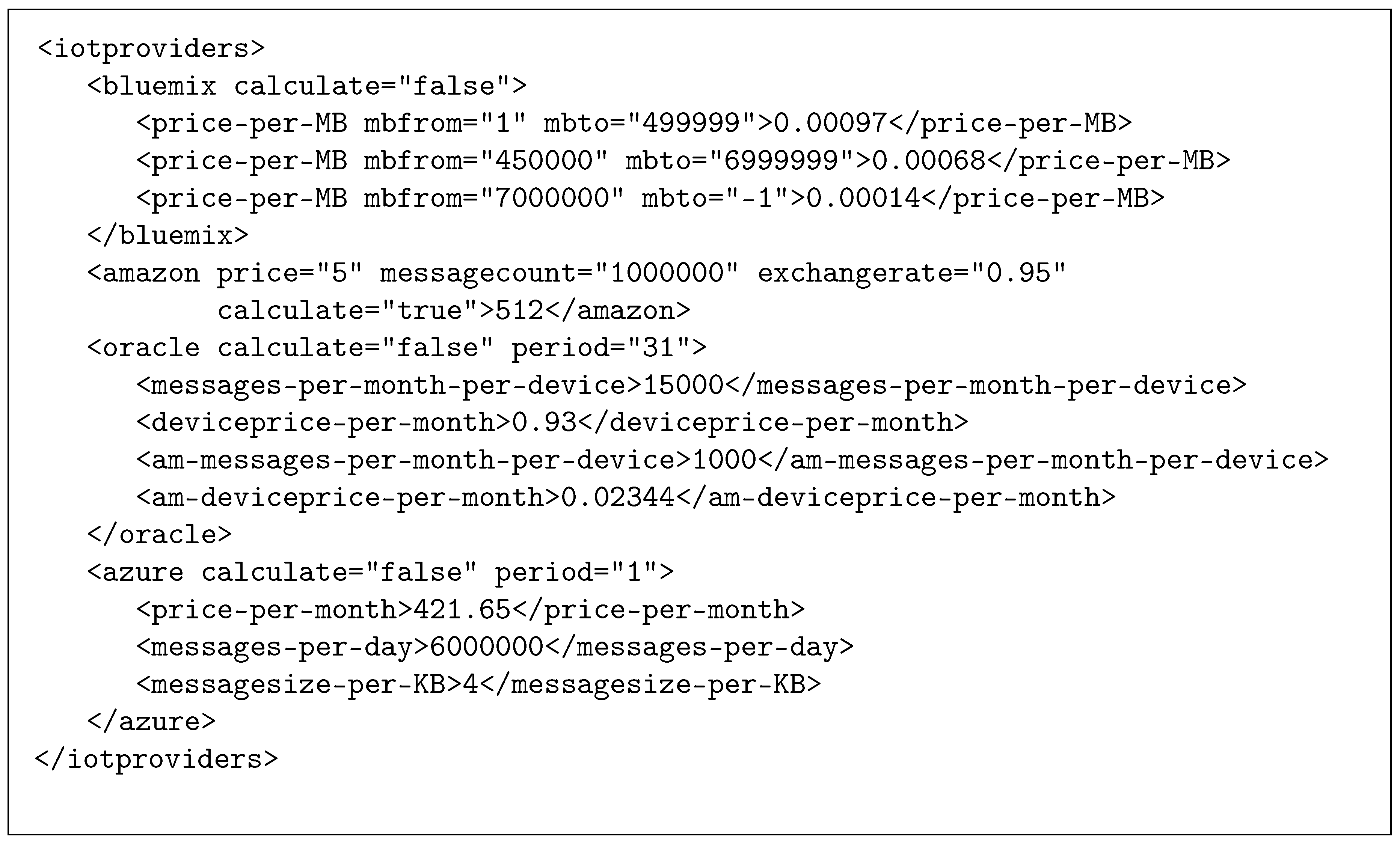
Based on these investigations, we created a cost model for IoT systems (represented by the IoT Pricing component in Figure 1), in which the IoT usage prices can be represented in an XML (Extensible Markup Language) format. Figure 2 shows its structure and the concrete values for the applied categories. We use this description as a configuration file for implementing and executing cost-based experiments in the simulator. We manage all prices in Euro. Some providers publish costs in US dollars (like Amazon)—in these cases, we apply conversion; therefore, we also have to specify an exchange rate to Euros. The first line contains the size and target attributes, which are used to define a VM/container specification for the simulation, and name a provider to be used for price calculation, respectively. In the second line, we define the pricing scheme for Bluemix, which is solely based on the data transferred. From the 7th line, we define the scheme of Amazon, which the provider charges after the number of messages sent. Here, we denoted that one million messages cost 5 dollars, and the exchange rate to Euros, which is . The maximum size of a message is 512 bytes. From the 9th line, we define Oracle’s scheme. It defines the maximum number of messages to be sent by a device (15,000), and a price for handling a device from this category (). Once additional messages need to be sent, there is an extra charge, Euros per 1000 messages. The period attribute defines the time interval for monitoring in days. Finally, from the 15th line, the Azure scheme is defined, which restricts the number of messages to be sent in a day (6,000,000) and the message size (4 KiB), and defines a monthly price for this service ().
To handle both IoT and cloud costs, we created another cost model that represents the cloud usage prices (represented by the Cloud Pricing component in Figure 1). Figure 3 shows the XML structure and the cost values for the applied categories. This configuration file contains some providers (for example, the amazon element starting in the second line), and the defined values are based on the gathered information from the providers’ public websites discussed before. We specified three different sizes for applicable VMs (named small, medium and large). This XML file has to contain at least that size category, which was defined by the size attribute in the IoT XML provider configuration file. As we can see from the fourth line to the seventh line, a category defines a virtual machine with the given ram and cpucores attributes, and we state the virtual machine prices with the instance-price and hour-per-price attributes. If we select the Amazon provider with a small category, then, in the scenarios, a virtual machine will have 1 CPU core and 2 GB of RAM, and the usage of this virtual machine will cost Euro per hour.
4. Implementation and Validation
Based on the generic, architectural plans introduced in Section 3 we implemented a model of a real-world IoT system in the extended DISSECT-CF simulator. As meteorology and weather forecasting were pioneers of sensor networks, our choice for the real-world system was a crowdsourced meteorological service [6]. This service is one of the most popular websites on meteorology in Hungary providing weather updates every 10 minutes and forecasts for up to a week. Our aim in this section is to evaluate the likely behaviour of the data collection and pre-filtering techniques behind the system and analyse the potential costs of utilising cloud provided IoT processing facilities for these operations.
Figure 4 details our implementation, which revolves around the classes of the Application and the Station (these are implementations of the IoT Controller and Sensor components from Figure 1). The Station acts as a gateway of interconnected sensors, while the Application implements custom IoT cloud use cases by examining various management and processing algorithms of sensor data in VMs of a specific cloud environment. Station provides the sensors’ network connection (e.g., towards the VMs used by the Application) and optimises their bandwidth utilisation by caching and bundling outgoing metering data. This caching behaviour is governed by the Application’s tasksize attribute.
The Provider class is the implementation of the IoT Pricing and Cloud Pricing components of the architecture shown in Figure 1). In the previous section, we defined our proposed cost model with two XML-based, declarative modelling language schemes for representing and configuring IoT and cloud side costs of certain providers. These samples can be used to assign pricing to the corresponding entities within the simulation, and the Provider class is responsible to load (i.e., read) and manage these values for cost calculations. It can be specified for each simulated IoT cloud system and which provider (thus pricing scheme) to be used for the calculation. If one needs to define a new IoT provider (other than the ones introduced), then the abstract class of Provider needs to be extended with an overridden method called: IoTCostCounter(). This extension can use the existing elements of the XML to define its new scheme. If a completely new method is needed for cost calculation, then the relevant XML parsing must also be done by the extension. To define a new cloud provider, one has to change the target and the size attributes (defined in the IoT provider XML file) and keep it in sync with the cloud provider XML file. This could entail the overriding of the CloudCostCounter() method.
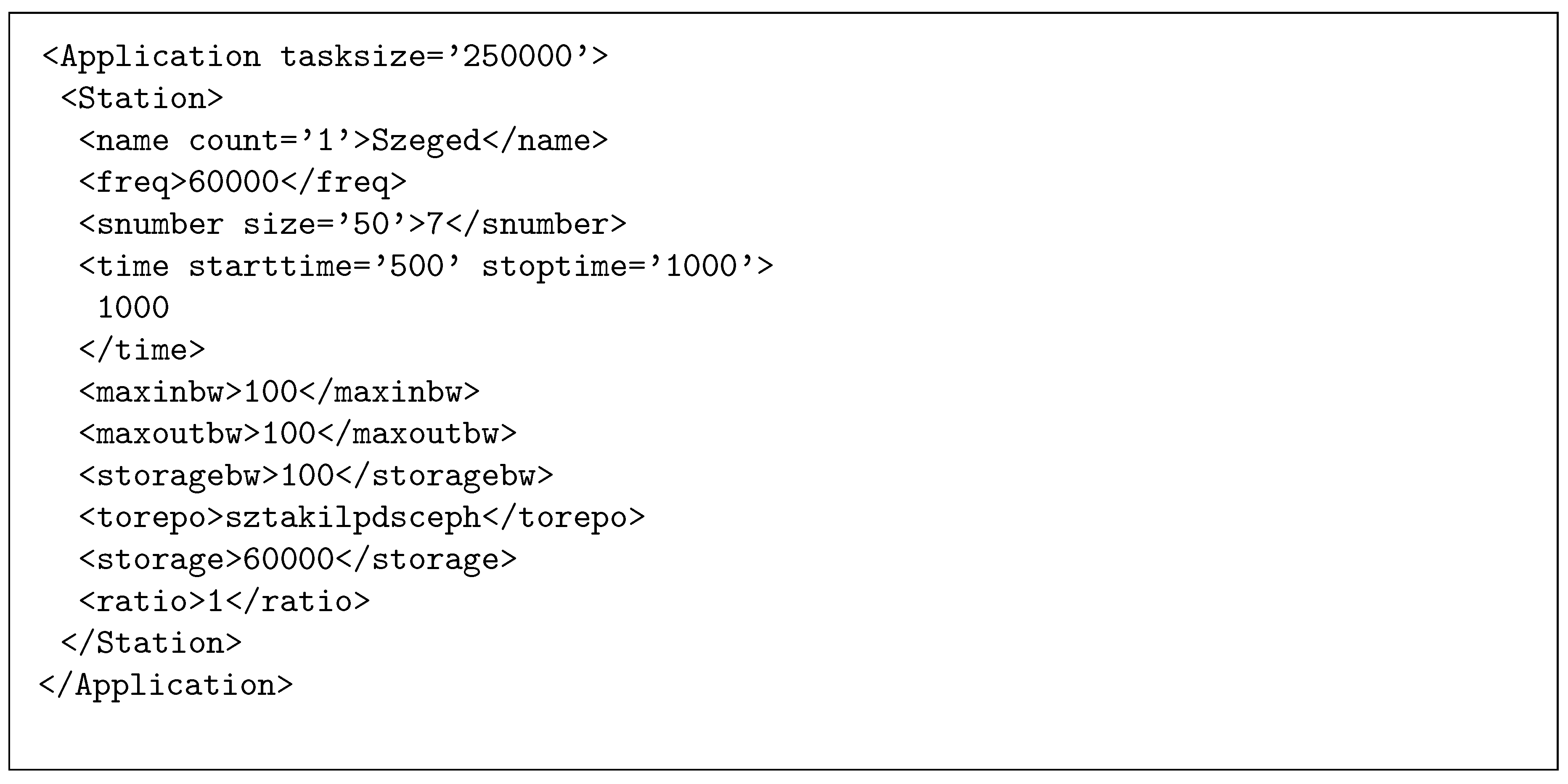
Figure 5 depicts the data representation of stations in our model. Stations have unique identifiers (i.e., a name) representing a weather station. Their lifetime can be specified with the tag time by defining their starttime (the time of their first activity) and stoptime (the time of their last activity). These details are configured for each use case specifically. The cardinality of the station’s supervised sensor set is set via sbnumber. Alongside the set cardinality, one can also specify the average data size produced by one of the sensors in the set.
In our experiments, sbnumber and size are set according to specifications of the weather stations on sale by idokep.hu. They sell these to improve the service’s sensor network and weather predictions via crowd sourcing. These stations have sensors to monitor at most the following environmental properties: (i) air and dew point temperature (in °C); (ii) humidity (%); (iii) barometric pressure (hPa); (iv) rainfall (mm/hour and mm/day); (v) wind speed (km/h); (vi) wind direction; (vii) and UV-B level. In summary, data packets from a single station are estimated to be approximately 50 bytes/measurement [25].
To set up more stations with the same properties, one can use the count option in the name tag. This option allows experiments to determine how the Application reacts to various sized sensor swarms. To realistically represent the modelled weather service, we set this value to 503 as this is their currently operated station count Station count collected on 01/04/2017. Data generation frequency (freq) could be set for the sensor set (in milliseconds). The station’s caching mechanism is influenced with the tag ratio. This defines the amount of data to be kept at the local storage relative to the average dataset produced by the sensors at each data generation event. If the cached data in the local storage (i.e., storage) overreaches its limit, the station models the transfer of the data to the cloud storage (specified in the torepo tag). The station’s network bandwidth to the outside world is specified by the tags maxinbw and maxoutbw.
In the implementation, the Cloud class is used to specify and set up a cloud environment (i.e., allows the simplified creation and configuration of IaaSService objects). The alternative, to-be-evaluated scenarios should be defined by the Application class. The VmCollector class can be used to manage the VMs backing the Application’s computing activities. Its two important methods are: VmSearch() matches tasks with free VMs—i.e., defines the load balancing strategy of the application; and the generateAndAdd() can be used to deploy a new VM—i.e., it provides the implementation for the auto-scaler for the application.
Next, we detail the generic steps followed by our Application implementation which has XML based customisation for application behaviour. This inner working is also depicted in Figure 6. By executing a simulation, the following steps are taken:
- Step 1: Set up the cloud using an XML. As we expect meteorological scenarios will often use private clouds, we used the model of a Hungarian private infrastructure (the LPDS (Laboratory of Parallel and Distributed Systems) Cloud of MTA SZTAKI (Institute for Computer Science and Control, Hungarian Academy of Sciences).
- Step 2: Set up the necessary amount of stations (using a scenario specific XML description) with the previously listed eight sensors per station.
- Step 3: Load the VM parameters from XML files, which also describe the cloud and IoT costs. Start the Application to deploy an initial VM (generateAndAddVM()) for data processing and to start the metering process in all stations (startStation()).
- Step 4: The stations then monitor (Metering()), save and send (startCommunicate()) sensor data (to the cloud storage) according to their XML definition. Parallel to this, CloudCostCounter() and IoTCostCounter() methods estimate the price of IoT and cloud operation, based on the generated data and processing of those data. The process of cost calculation depends on the chosen provider. If provider pricing is not time-dependent, like in case of Bluemix, we have to pay only after data traffic, then this loop is executed only once, at the end of the simulation. Otherwise, if the provider cost is time-dependent, the time interval for the measurements is given in the period attribute, as shown in Figure 2. This interval represents the frequency value to be used by the extended provider class, and the corresponding cost counter methods are executed in all cycles.
- Step 5: A daemon service checks regularly if the cloud repository received a scenario specific amount of data (see the tasksize attribute in Figure 5). If so, then the Application generates the ingest compute tasks, which will finish processing within a predefined amount of time.
- Step 6: Next, for each generated task, a free VM is searched (by VmSearch()). If a VM is found, the task and the relevant data is sent to it for processing.
- Step 7: In case there are no free VMs found, the daemon initiates a new VM deployment and holds back the not yet mapped tasks.
- Step 8: If at the end of the task assignment phase, there are still free VMs, they are all decommissioned (by turnoffVM()), except those that are held back for the next rounds (this amount can be configured and even completely turned off at will).
- Step 9: Finally, the Application returns to Step 5.
Evaluation with Five Scenarios
In this sub-section, we reveal five scenarios addressing questions likely to be investigated with the help of extended DISSECT-CF [26]. Namely, our scenarios mainly focus on how resource utilization and management patterns alter based on changing sensor behaviour and how do these affect the incurred costs of operating the IoT system (e.g., how different sensor data sizes and varying number of stations and sensors affect the operation of the simulated IoT system). Note, the scope of these scenarios is solely focused on the validation of our proposed IoT extensions and thus the scenarios are mostly underdeveloped in terms of how a weather service would behave internally.
Before getting into the details, we clarify the common behavioural patterns, we used during all of the scenarios below (these were the common starting points for all scenarios unless stated otherwise). First of all, to limit simulation runtime, all of our experiments limited the station lifetimes to a single day. The start-up period of the stations were selected randomly between 0 and 20 min. The task creator daemon service of our Application implementation spawned tasks after the cloud storage received more than 250 KiB of metering data (see the tasksize of Figure 5). This step ensured the estimated processing time of 5 min/task. The cloud storage was completely run empty by the daemon: the last spawned task was started with less than 250 KiB to process—scaling down its execution time. The application was mainly using Bluemix Large VMs (see Figure 3). Finally, we disabled the dynamic VM decommissioning feature of the application (see step 8 in Section 4).
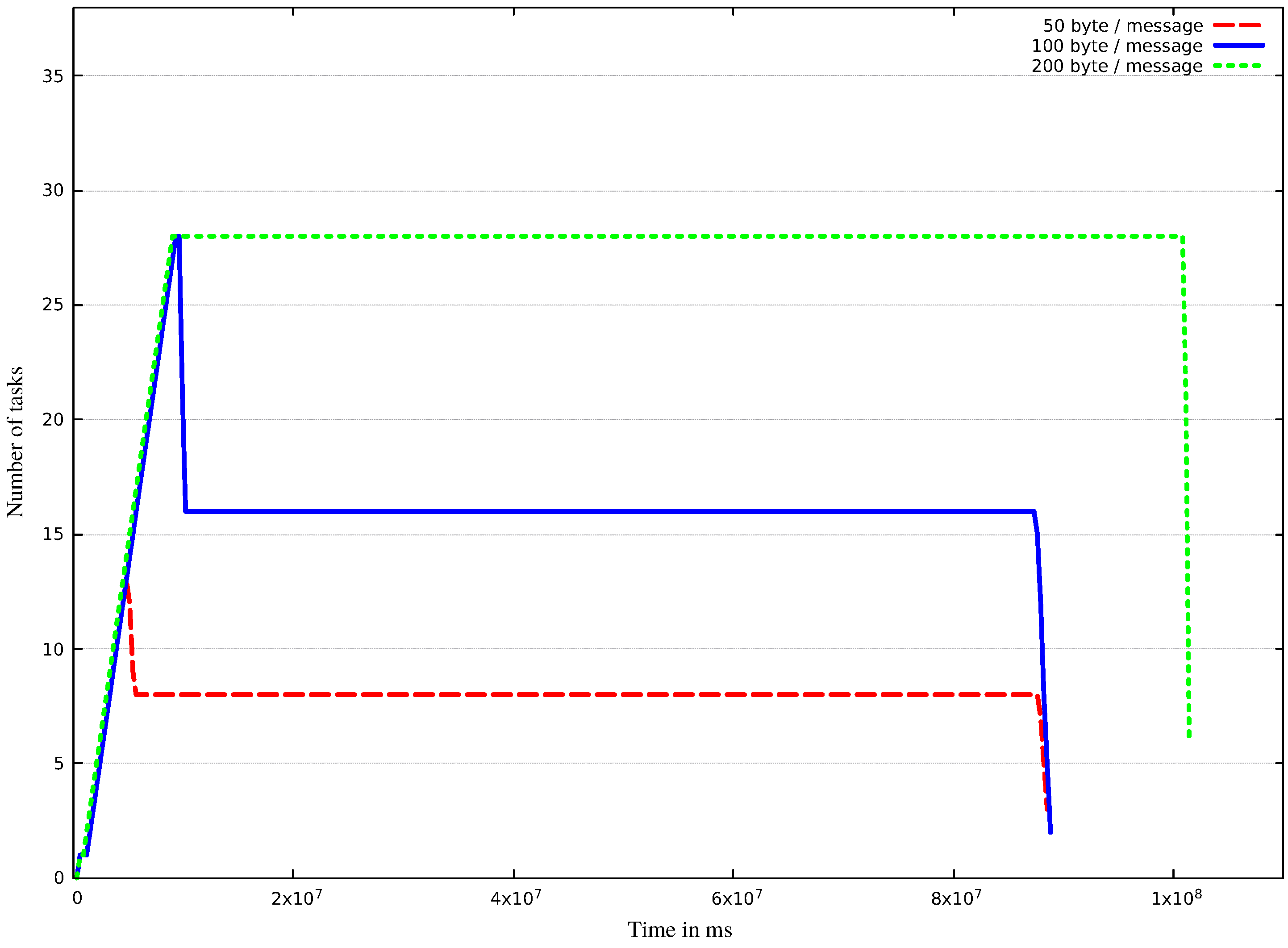
In scenario N, we varied the amount of data produced by the sensors: we set 50, 100 and 200 bytes for different cases (allowing overheads for storage, network transfer, different data formats and secure encoding etc.). We simulated all stations of the weather service for 24 h. We also investigated how the costs of the IoT side changed, if we would use one of the four IoT providers defined before. The measurement results can be seen in Figure 7 and Figure 8, and Table 1. For the first case with 50 bytes of sensor data, we measured 0.261 MiB of produced data in total, while in the second case of 100 bytes we measured 0.522 MiB, and in the third of 200 bytes we measured 1.044 GBs (showing linear scale up). In the three cases, we needed 12, 27 and 28 VMs to process all tasks, respectively. With the preloaded cloud parameters, the system is allowed to start maximum 28 virtual machines; therefore, in the first case of 50 bytes, our cloud cost was Euros, in the second case of 100 bytes, the cloud cost was , and finally, in the last case, our cloud cost was Euros. The lessons learnt with this scenario is that, if we use more than 200 bytes per message, we need stronger virtual machines (also a larger cloud with stronger physical resources) to manage our application because, in the third case, the simulation runs for more than 24 h (despite the sensors were only producing data for a single day), which increased our costs using time-dependent cloud services. Finally, Table 1 shows how much virtual machines needed to process all of generated data for all test cases, and how much tasks were generated for the produced data.
Figure 8 presents a cost comparison for all considered providers. We can see that Oracle costs are much higher than the other three providers in all cases (50, 100, 200 bytes messages). The main cause for this issue is that Oracle charges after each utilized device, which is not the case for other providers. Our initial estimations show that only such an IoT cloud system operation is beneficial with Oracle that has at most 200 devices and transfers 1–2 messages per minute per device.
In scenario N, we wanted to examine the effects of varying sensor numbers and varying sensor data sizes per stations to mimic real world systems better. Therefore, we defined a fixed case using 744 stations having seven sensors each, producing 100 bytes of sensor data per measurement, and a random case, in which we had the 744 stations with randomly sized sensor set (ranging between 6–8) and sensor data size (50, 100 or 200 bytes/sensor). The results can be seen in Figure 9 and Figure 10 and Table 2. As we can see, we experienced minimal differences; the random case resulted in slightly more tasks. Furthermore, there are minimal differences between the cost of IoT providers, but we can see that even the small configuration differences can cause bigger variations of the costs, like in the case of Amazon. Table 2 shows how much virtual machines needed to process all generated data, and how many tasks were generated by the produced data in fixed and random cases.
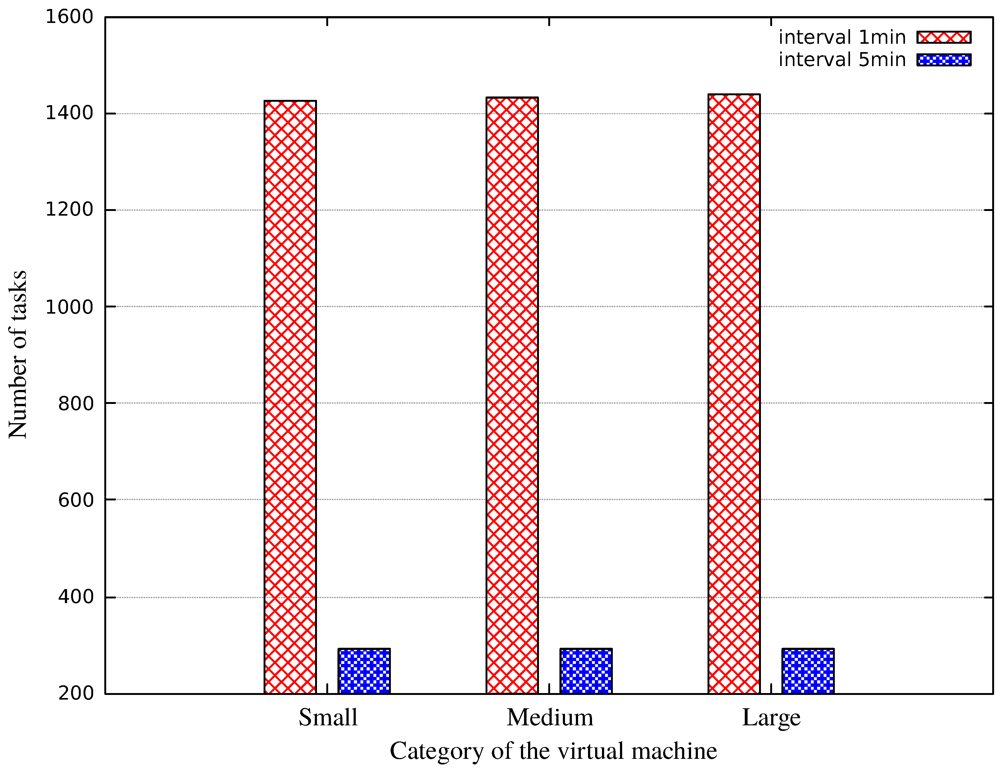
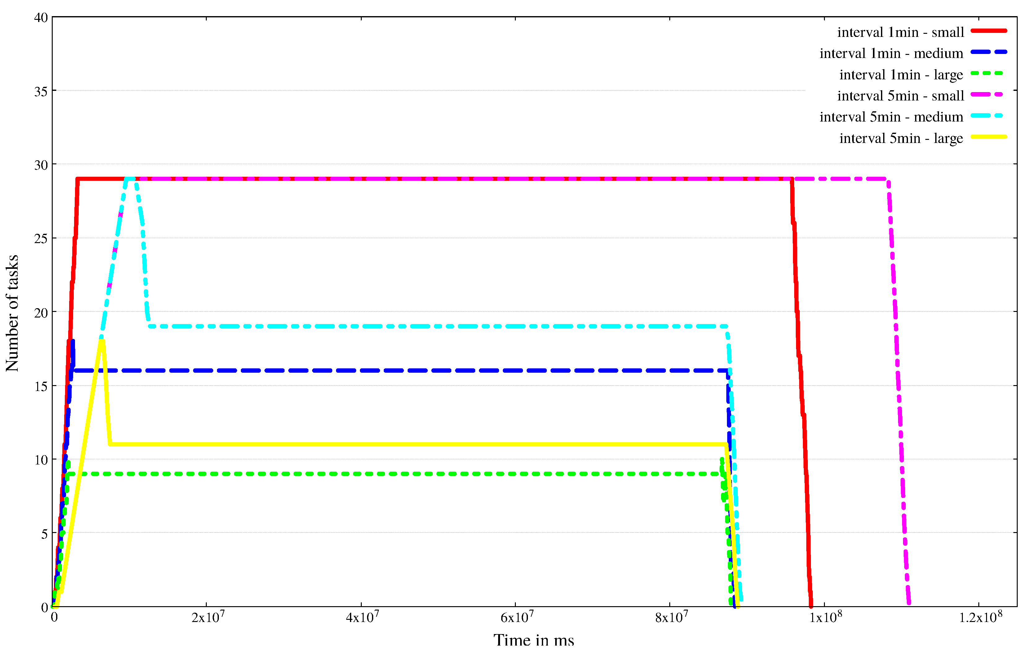
In scenario N, we examined two sensor data generation frequencies. We set up 600 stations and defined cases for two static frequencies (1 and 5 min). In real life, the varying weather conditions may call for (or result in) such changes. In both cases, the sensors generated our previously estimated 50 bytes. The results can be seen in Figure 11, Figure 12 and Figure 13 and in Table 3, Table 4 and Table 5. The generated data in total: 0.321 GiB for 1 min frequency, 0.064 GiB for 5 min frequency. In this scenario, we used the three categories (small, medium and large) of the Azure cloud provider for both data generation frequencies. The first category contains 1 core and 1.75 GiB memory, the second contains two cores and 3.5 GiB memory, and finally we defined a virtual machine with eight cores and 14 GiB memory for the third category. The application needs more than 1400 tasks to process all generated data by the stations with 1 min frequency, while the data generated by stations with 5 min frequencies needed almost 300 tasks to process them. For this work, the application deployed 75 VMs with the small category by the Azure cloud provider in the 1 min case, and 10 VMs in the 5 min case. For medium category VMs, we needed 41 in the 1 min case, and five VMs in the 5 min case. Finally, 15 large category VMs needed to process in time for the 1 min case, but only one virtual machine was necessary to process all data generated in the 5 min case. As we can see from the results, the cheapest choice for operating the IoT side is Bluemix.
To summarize, with this scenario, we have shown how small changes in the system parameters can affect the number of the virtual machines needed for sensor data processing, and the measurements also reflected how these parameters affect the final usage prices. Table 3, Table 4 and Table 5 show the detailed costs of the three test cases. The IoT costs are the same in all cases, but, from the cloud side costs, we can see that the stronger virtual machine we use, the more we should pay to operate the system.
In the three scenarios executed so far, the main application was responsible for processing the sensor data in the cloud and checked the repository for new transfers in every minute. In some cases, we experienced that only a small amount of data has arrived within this interval (i.e., task creation frequency). Therefore, in scenario N, we examined what happens if we widen this interval to 5 min. We executed it with 487 stations. The results can be seen in Figure 14, Figure 15, Figure 16 and Figure 17. In this scenario, we used the Oracle cloud provider pricing to calculate the cloud side costs for the running virtual machines. In this simulation we had three categories: 75 (small), 139 (medium) and 268 Euros (large) for one instance of a VM, and we wanted to know which provider offers the cheapest prices if we use 1 min frequency or 5 min frequency for task generation. In all six test cases, we had similar IoT costs as shown in Figure 14, and the best provider is Bluemix with 0.259 Euros. Figure 16 shows that we can save money if we choose the small category with 1 min interval or the small category of 5 min interval because they have the cheapest cloud costs with Euros. The disadvantage of these categories (which was presented by Figure 15) is that we needed more time to process all generated data than in the case of the other categories. Finally, in Figure 17, we can see that the number of tasks is almost equal, but we needed different numbers of virtual machines to process these tasks. We can summarize that increasing the processing time is not always the best solution for application management and for saving money.
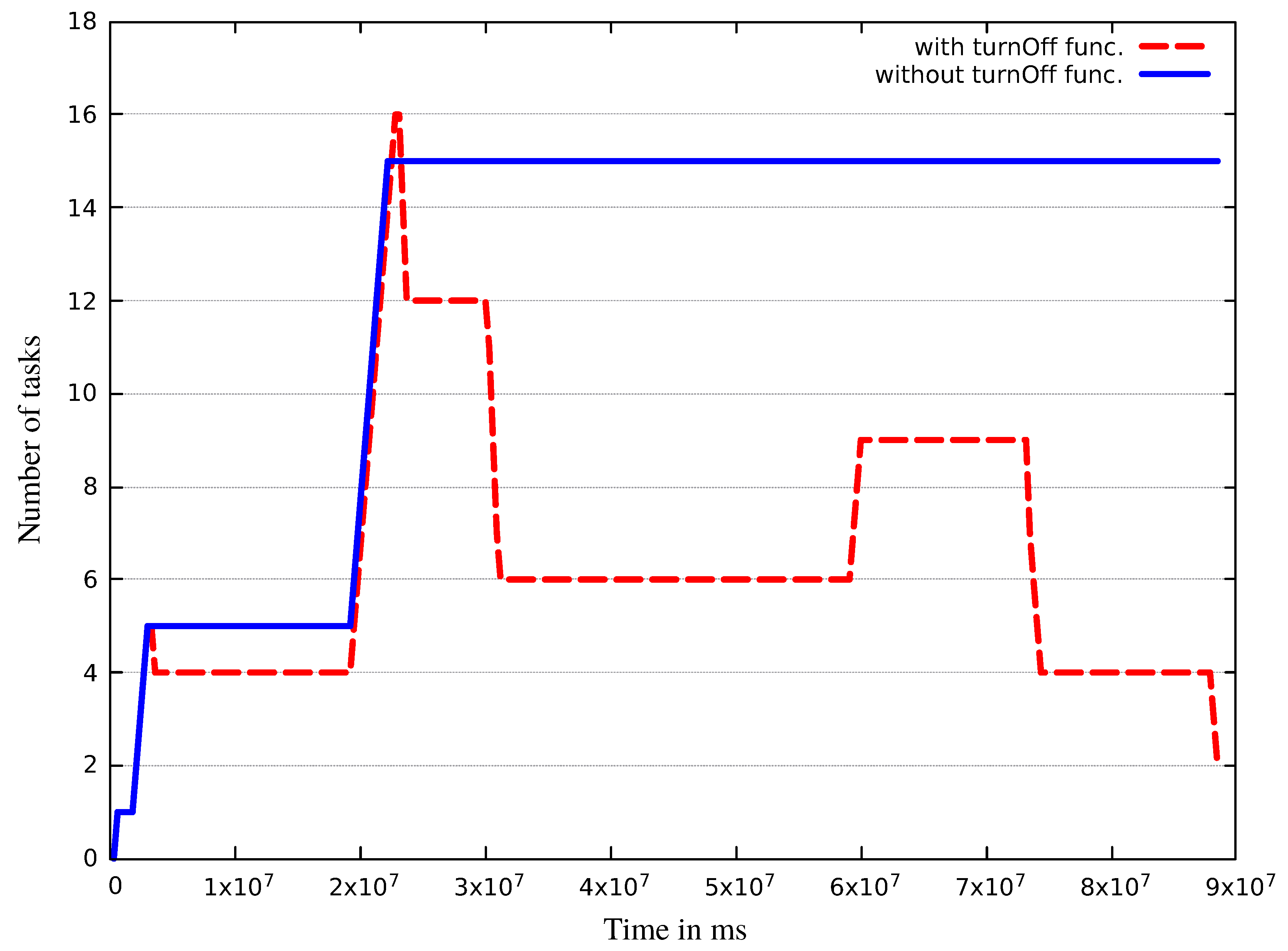
As we model a crowdsourced service, we expect to see a more dynamic behaviour regarding the number of active stations. In the previous cases, we used a static number of stations per experiment, while in our final scenario, N, we ensured the station numbers to dynamically change. Such changes may occur due to station or sensor failures, or even by sensor replacement. In this scenario, we performed these changes by specific hours of the day: from 12:00 a.m. to 5:00 a.m., we started 200 stations, from 5:00 a.m. to 8:00 a.m., we operated 700 stations, from 8:00 a.m. to 4:00 p.m., we scaled them down to 300, then from 4:00 p.m.to 8:00 p.m. Up to 500, finally, in the last round from 8:00 p.m. to 12:00 a.m., we set it back to 200. In this experiment, we also wanted to examine the effects of VM decommissioning; therefore, we executed two different cases, one with and one without turning off unused VMs. In both cases, we set the tasksize attribute to the usual 250 KiB. The results can be seen in Figure 18. We can see that, without turning off the unused VMs from 6:00 p.m., we kept 15 VMs alive (resulting in more over provisioning), while, in the other case, the number of running VMs dynamically changed to the one required by the number of tasks to be processed.
Table 6 shows what happens with the application operating costs, if we do not turn off the unused, but still running virtual machines. The cheapest IoT provider is Bluemix with Euros, and we can save almost 38 Euros using the VM turnOff function. If we used Oracle as the cloud provider, we would pay for a virtual machine instance of the smallest category 75 Euros, resulting in 1125 Euros for operating the cloud side of our application.
As a summary, in this section, we presented five scenarios focusing on various properties of IoT cloud systems. We have shown that, with our extended simulator, we can investigate the behaviour and operating costs of these systems and contribute to the development of better design and management solutions in this research field.
5. Conclusions
Distributed systems simulators are not generic enough to be applied in newly emerging domains, such as IoT Cloud systems. These simulators are often limited in their details, extensibility and support for the to be modelled IoT devices. Therefore, in this paper, we introduced a method to show how generic IoT sensors could be modelled in a state-of-the-art cloud simulator. We showed how the fundamental properties of IoT entities can be represented in the simulator, and proposed an XML based, declarative modelling language to describe the behaviour of various sensors.
We also enabled the investigation of operating costs of IoT scenarios by introducing a model of provider pricing schemes to the simulator. Finally, we validated our extensions in the simulator by executing five different scenarios of simulated IoT systems provisioning a meteorological service.
Our future work will address investigations on non-frequency based sensor data production to allow more influence on when and what kind of data is produced by a particular sensor. In addition, an initial model for sensors and actuators on geographical location will be proposed. As a result, the simulations could incorporate moving devices that could change their behaviour according to their locations (e.g., modelling of network quality changes based on location).
Supplementary Materials
This paper described the behaviour and features of DISSECT-CF version 0.9.8. Its source code is open and available (under the licensing terms of the GNU LGPL 3) at the following website: https://github.com/kecskemeti/dissect-cf.
Acknowledgments
This research was supported by the EU-funded Hungarian national grant GINOP-2.3.2-15-2016-00037 titled ”Internet of Living Things”, and by the European COST programme under an Action identifier IC1304 (ACROSS). This paper is a revised and extended version of the conference paper [27].
Author Contributions
Attila Kertesz and Gabor Kecskemeti concieved the ideas for the DISSECT-CF extensions and the experiments, Andras Markus implemented them and collected the measurements, finally, all authors contributed equally to the text of the paper.
Conflicts of Interest
The authors declare no conflict of interest.
References
- Sotiriadis, S.; Bessis, N.; Asimakopoulou, E.; Mustafee, N. Towards simulating the Internet of Things. In Proceedings of the IEEE 28th International Conference on Advanced Information Networking and Applications Workshops (WAINA), Cracow, Poland, 16–18 May 2014; pp. 444–448. [Google Scholar]
- Han, S.N.; Lee, G.M.; Crespi, N.; Heo, K.; Van Luong, N.; Brut, M.; Gatellier, P. DPWSim: A simulation toolkit for IoT applications using devices profile for web services. In Proceedings of the IEEE World Forum on IoT (WF-IoT), Seoul, Korea, 6–8 March 2014; pp. 544–547. [Google Scholar]
- Zeng, X.; Garg, S.K.; Strazdins, P.; Jayaraman, P.P.; Georgakopoulos, D.; Ranjan, R. IOTSim: A simulator for analysing IoT applications. J. Syst. Archit. 2016, 72, 93–107. [Google Scholar] [CrossRef]
- Kecskemeti, G. DISSECT-CF: A simulator to foster energy-aware scheduling in infrastructure clouds. Simul. Model. Pract. Theory 2015, 58P2, 188–218. [Google Scholar] [CrossRef] [Green Version]
- Kecskemeti, G.; Nemeth, Z. Foundations for Simulating IoT Control Mechanisms with a Chemical Analogy. In Internet of Things, Proceeding of the IoT 360° 2015, Rome, Italy, 27–29 October 2015. Revised Selected Papers, Part I; Mandler, B., Marquez-Barja, J., Eds.; Springer International Publishing: New York, NY, USA, 2016; Volume 169, pp. 367–376. [Google Scholar]
- Idokep.hu Website. Available online: http://idokep.hu (accessed on 13 August 2017).
- Sotiriadis, S.; Bessis, N.; Antonopoulos, N.; Anjum, A. SimIC: Designing a new Inter-Cloud Simulation platform for integrating large-scale resource management. In Proceedings of the IEEE 27th International Conference on Advanced Information Networking and Applications (AINA), Barcelona, Spain, 25–28 March 2013; pp. 90–97. [Google Scholar]
- Moschakis, I.A.; Karatza, H.D. Towards scheduling for Internet-of-Things applications on clouds: A simulated annealing approach. Concurr. Comput. 2015, 27, 1886–1899. [Google Scholar] [CrossRef]
- Silva, I.; Leandro, R.; Macedo, D.; Guedes, L.A. A dependability evaluation tool for the Internet of Things. Comput. Electr. Eng. 2013, 39, 2005–2018. [Google Scholar] [CrossRef]
- Khan, A.M.; Navarro, L.; Sharifi, L.; Veiga, L. Clouds of small things: Provisioning infrastructure-as-a-service from within community networks. In Proceedings of the IEEE 9th International Conference on Wireless and Mobile Computing, Networking and Communications (WiMob), Lyon, France, 7–9 October 2013; pp. 16–21. [Google Scholar]
- Calheiros, R.N.; Ranjan, R.; Beloglazov, A.; De Rose, C.A.; Buyya, R. CloudSim: A toolkit for modeling and simulation of cloud computing environments and evaluation of resource provisioning algorithms. Software 2011, 41, 23–50. [Google Scholar] [CrossRef]
- Botta, A.; De Donato, W.; Persico, V.; Pescapé, A. On the integration of cloud computing and internet of things. In Proceedings of the IEEE International Conference on Future Internet of Things and Cloud, Barcelona, Spain, 27–29 August 2014; pp. 23–30. [Google Scholar]
- Nastic, S.; Sehic, S.; Le, D.H.; Truong, H.L.; Dustdar, S. Provisioning software-defined iot cloud systems. In Proceedings of the IEEE International Conference on Future Internet of Things and Cloud, Barcelona, Spain, 27–29 August 2014; pp. 288–295. [Google Scholar]
- Giacobbe, M.; Puliafito, A.; Pietro, R.D.; Scarpa, M. A Context-Aware Strategy to Properly Use IoT-Cloud Services. In Proceedings of the 2017 IEEE International Conference on Smart Computing (SMARTCOMP), Hong Kong, China, 29–31 May 2017; pp. 1–6. Available online: http://dx.doi.org/10.1109/SMARTCOMP.2017.7946976 (accessed on 1 July 2017).
- DISSECT-CF Website. Available online: https://github.com/kecskemeti/dissect-cf (accessed on 13 August 2017).
- MS Azure IoT Hub Website. Available online: https://azure.microsoft.com/en-us/services/iot-hub (accessed on 13 August 2017).
- IBM Bluemix Website. Available online: https://www.ibm.com/cloud-computing/bluemix/internet-of-things (accessed on 13 August 2017).
- Amazon AWS IoT Website. Available online: https://aws.amazon.com/iot/pricing (accessed on 13 August 2017).
- Oracle IoT Platform Website. Available online: https://cloud.oracle.com/en_US/opc/iot/pricing (accessed on 13 August 2017).
- MS Azure Price Calculator. Available online: https://azure.microsoft.com/en-gb/pricing/calculator/ (accessed on 13 August 2017).
- IBM Bluemix Pricing Sheet. Available online: https://www.ibm.com/cloud-computing/bluemix (accessed on 13 August 2017).
- Amazon Pricing Website. Available online: https://aws.amazon.com/ec2/pricing/on-demand/ (accessed on 13 August 2017).
- Oracle Pricing Website. Available online: https://cloud.oracle.com/en_US/opc/compute/compute/pricing (accessed on 13 August 2017).
- Orcale Metered Services Pricing Calculator. Available online: https://shop.oracle.com/cloudstore/index.html?product=compute (accessed on 13 August 2017).
- Murdoch University Weather Station Website. Available online: http://wwwmet.murdoch.edu.au/downloads (accessed on 13 August 2017).
- DISSECT-CF Extension Scenarios. Available online: https://github.com/andrasmarkus/dissect-cf/tree/andrasmarkus-patch-1/experiments (accessed on 13 August 2017).
- Markus, A.; Kecskemeti, G.; Kertesz, A. Flexible Representation of IoT Sensors for Cloud Simulators. In Proceedings of the 25th Euromicro International Conference on Parallel, Distributed and Network-based Processing (PDP), St. Petersburg, Russia, 6–8 March 2017; pp. 199–203. [Google Scholar]
Figure 1.
The architecture of the extended DISSECT-CF simulator.

Figure 2.
Cost model of IoT providers.

Figure 3.
COST model of Cloud providers.
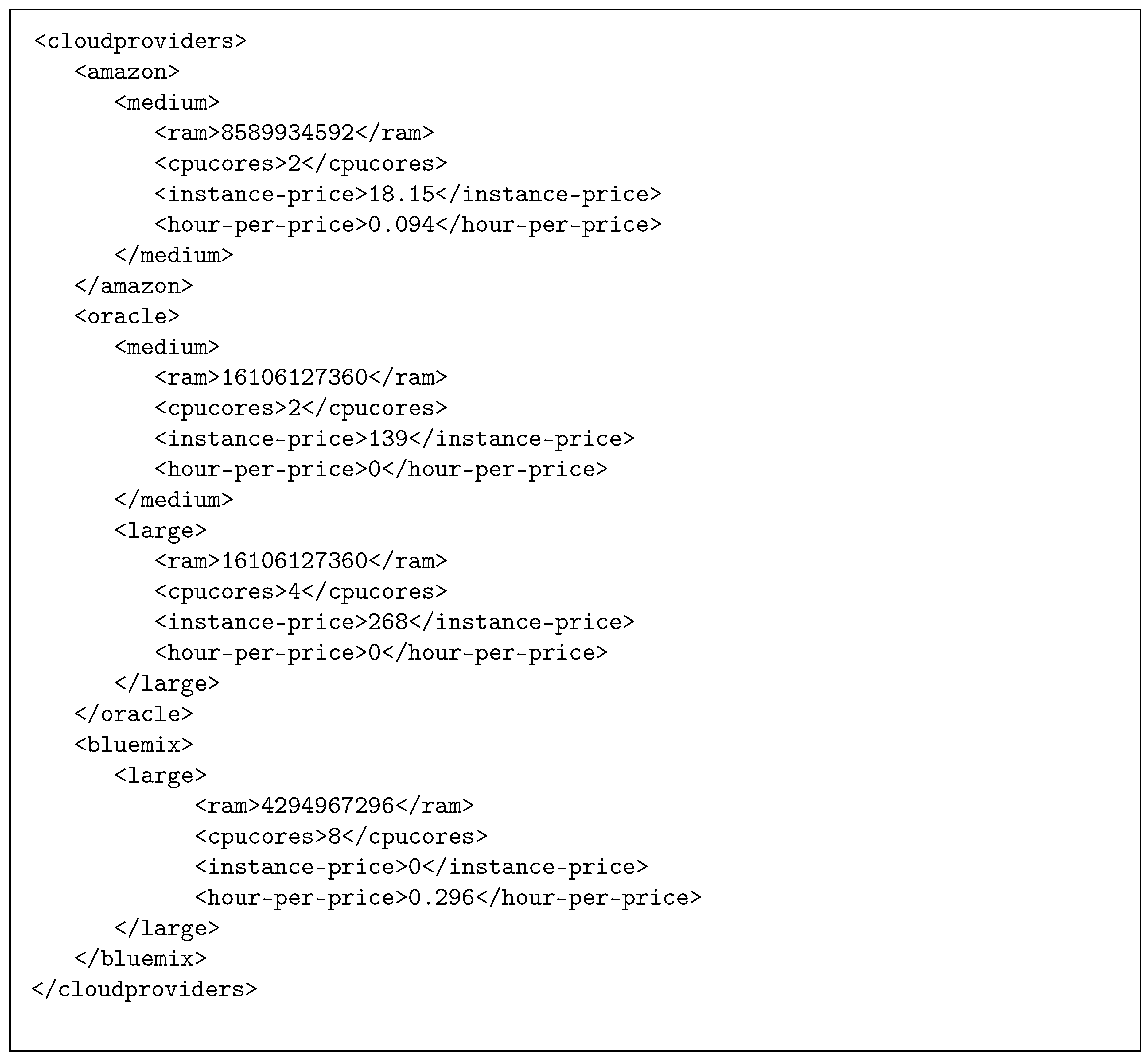
Figure 4.
IoT extension classes for DISSECT-CF.

Figure 5.
XML-based description of IoT systems.

Figure 6.
Sequence diagram of the application.
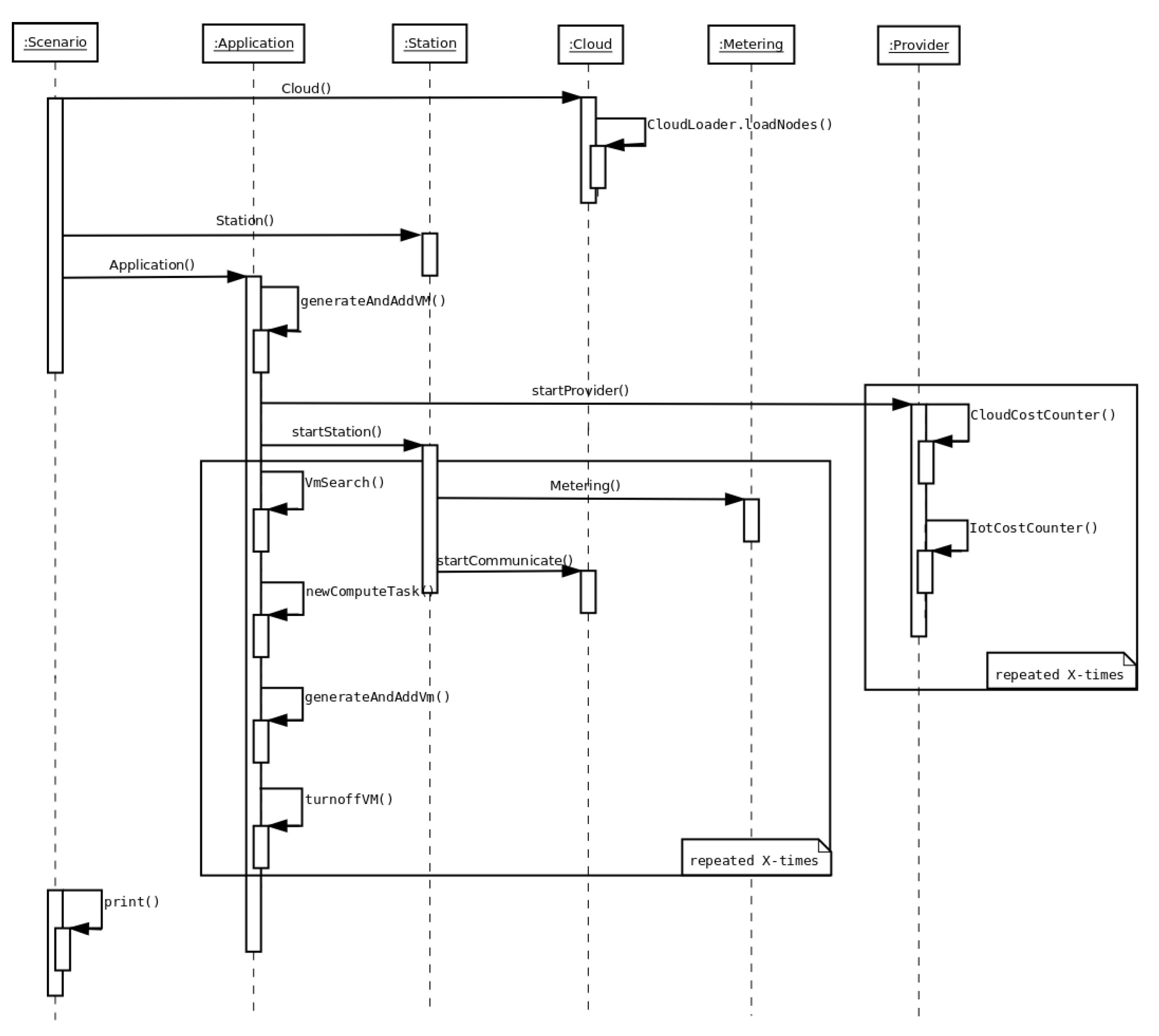
Figure 7.
Number of virtual machines in scenario N

Figure 8.
IoT and cloud costs in scenario N
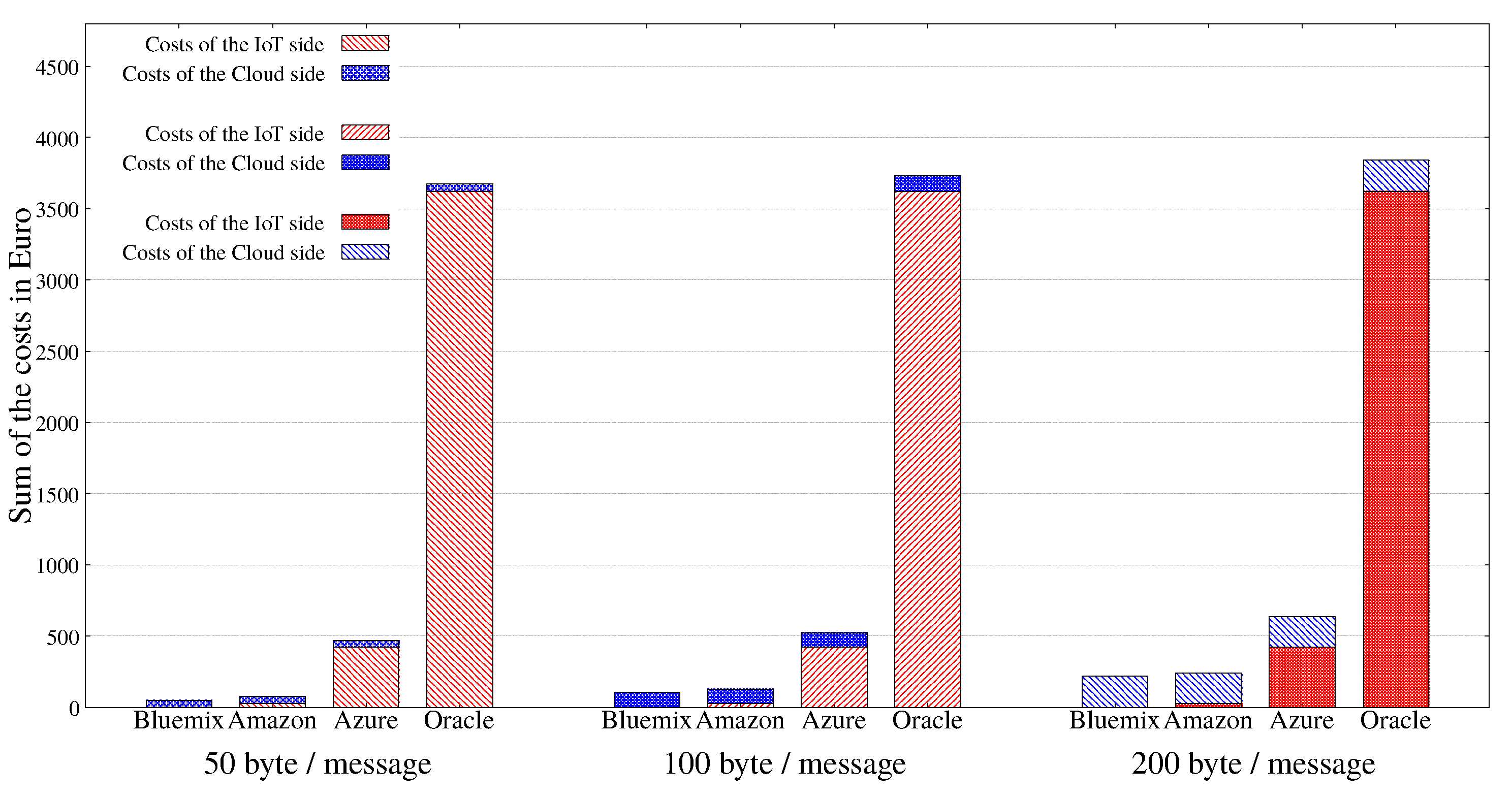
Figure 9.
Results of scenario N
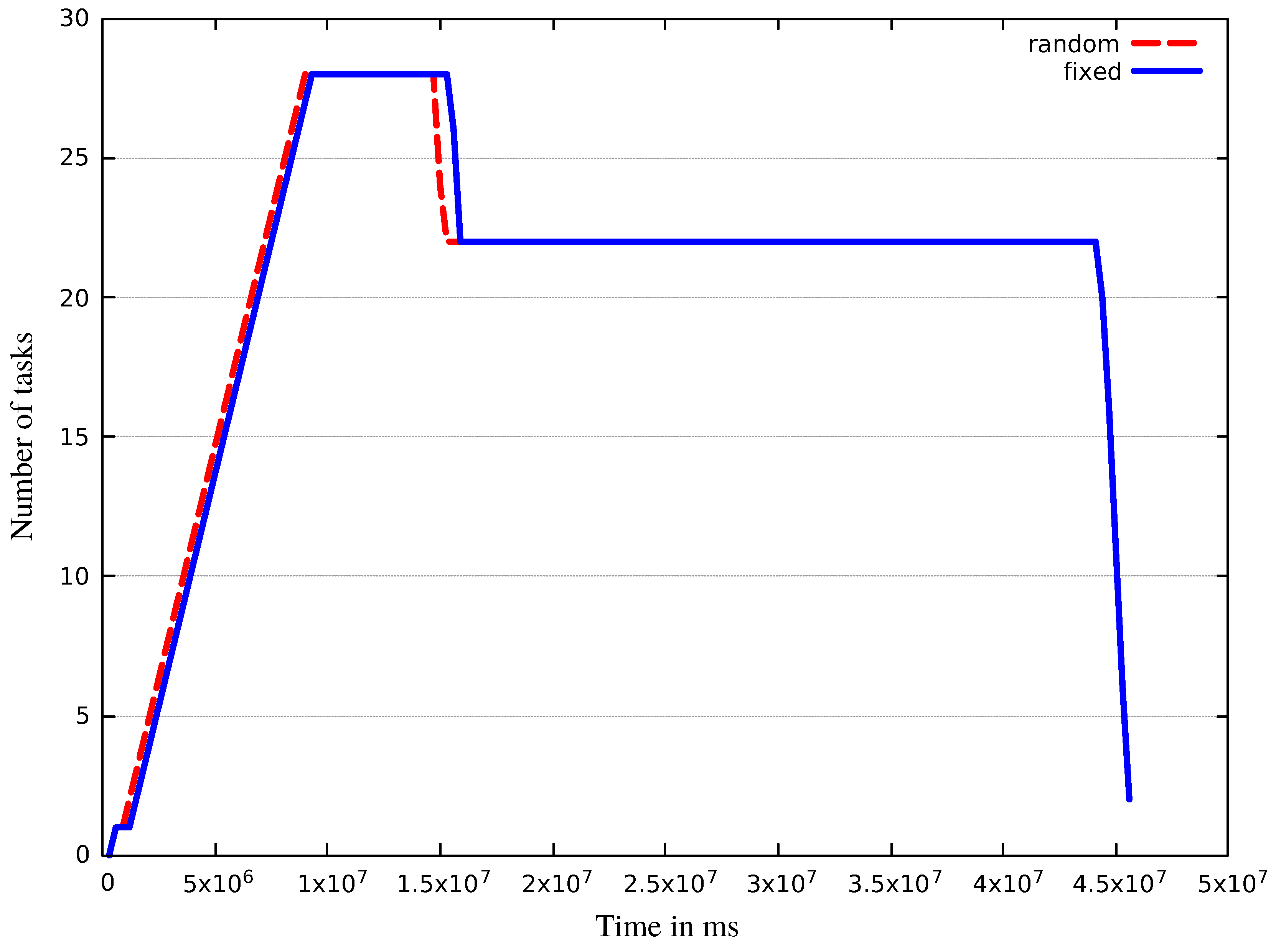
Figure 10.
Cost of the providers in scenario N
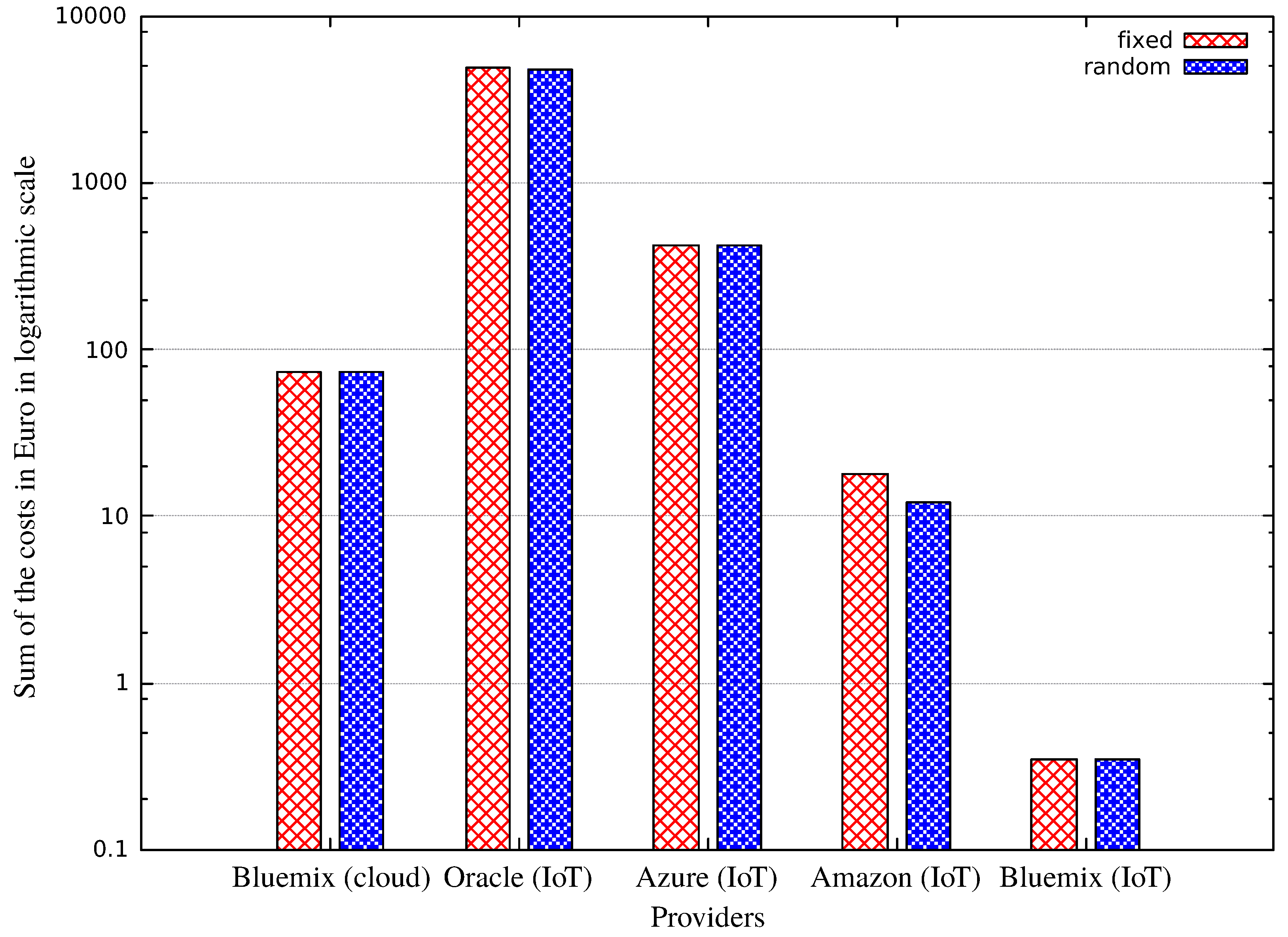
Figure 11.
Results of scenario N
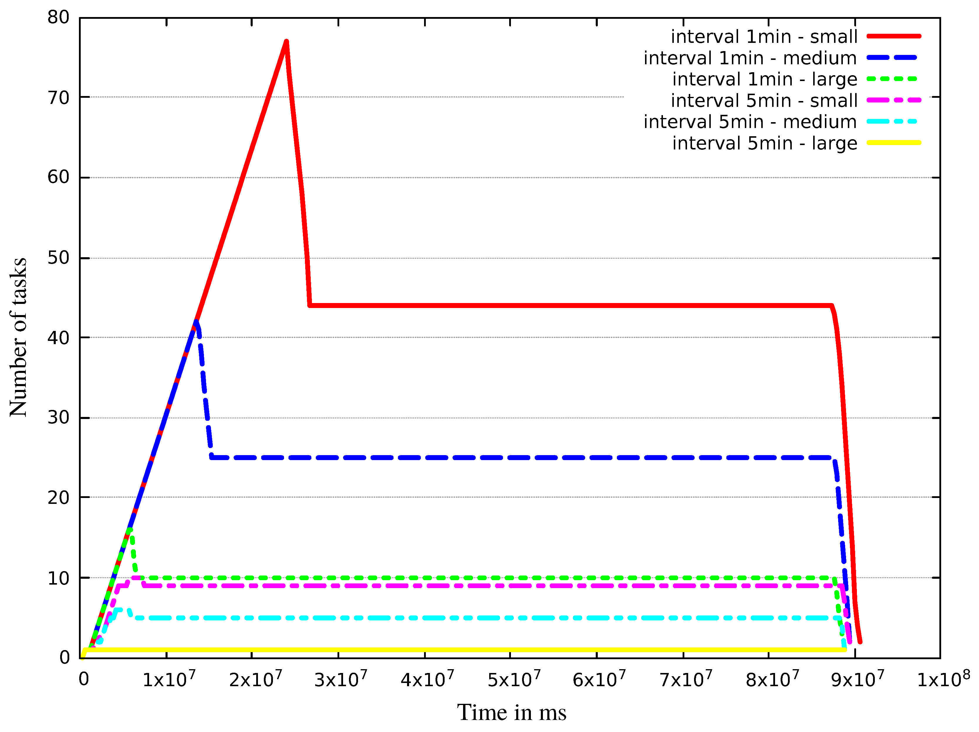
Figure 12.
Number of virtual machines in scenario N
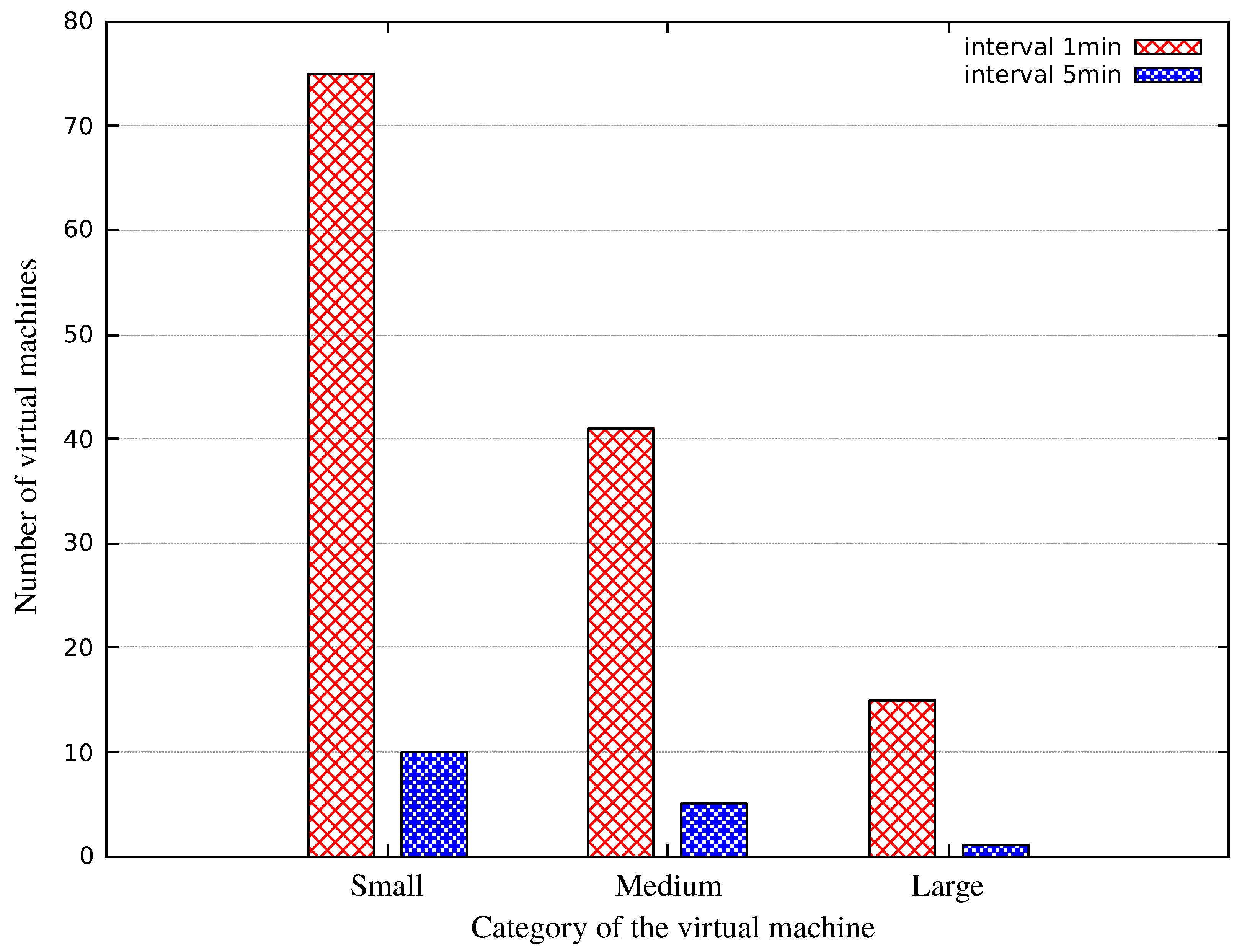
Figure 13.
Number of tasks over time in scenario N

Figure 14.
Cost of the IoT providers in N
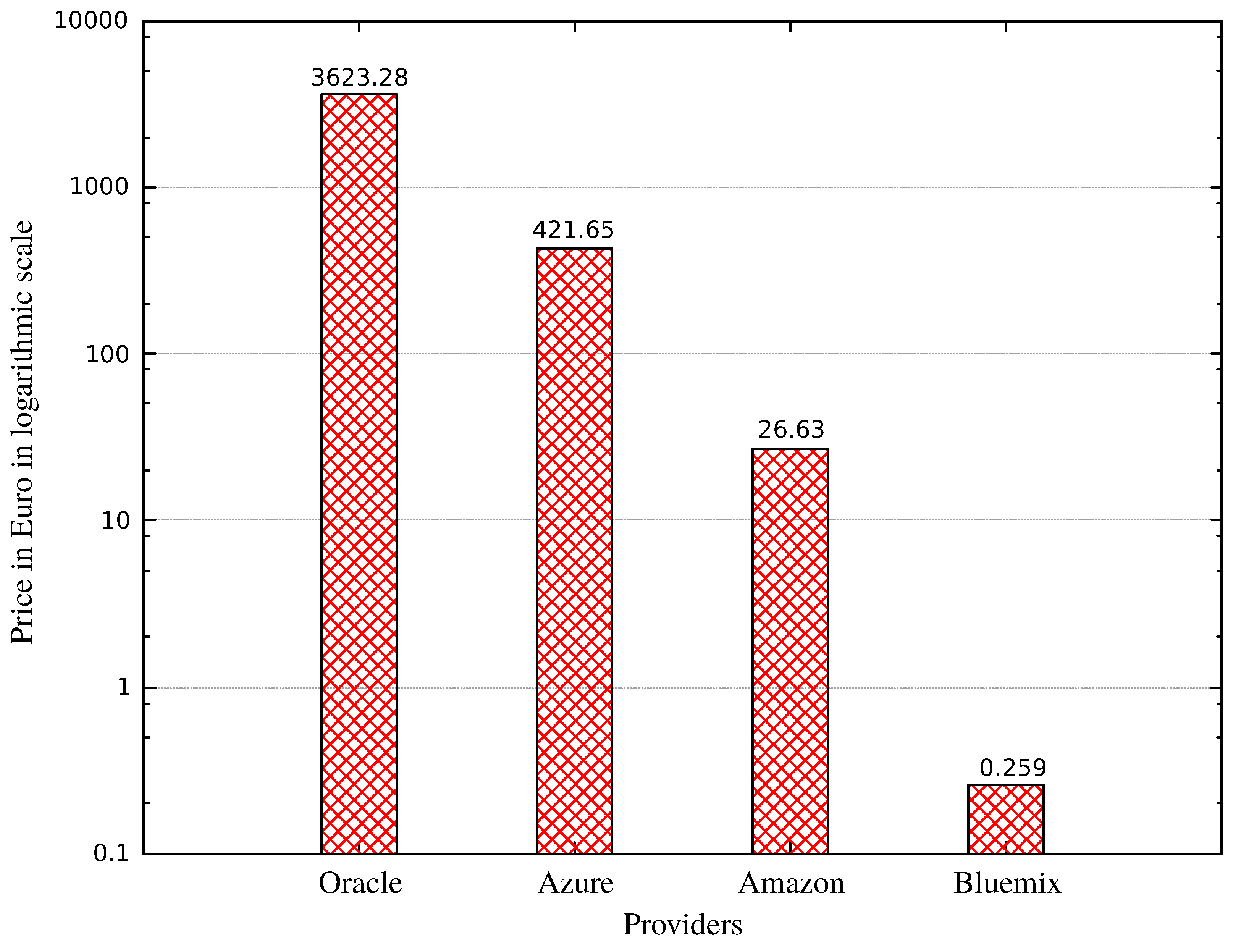
Figure 15.
Number of tasks in scenario N

Figure 16.
Cost of the Oracle cloud provider in scenario N
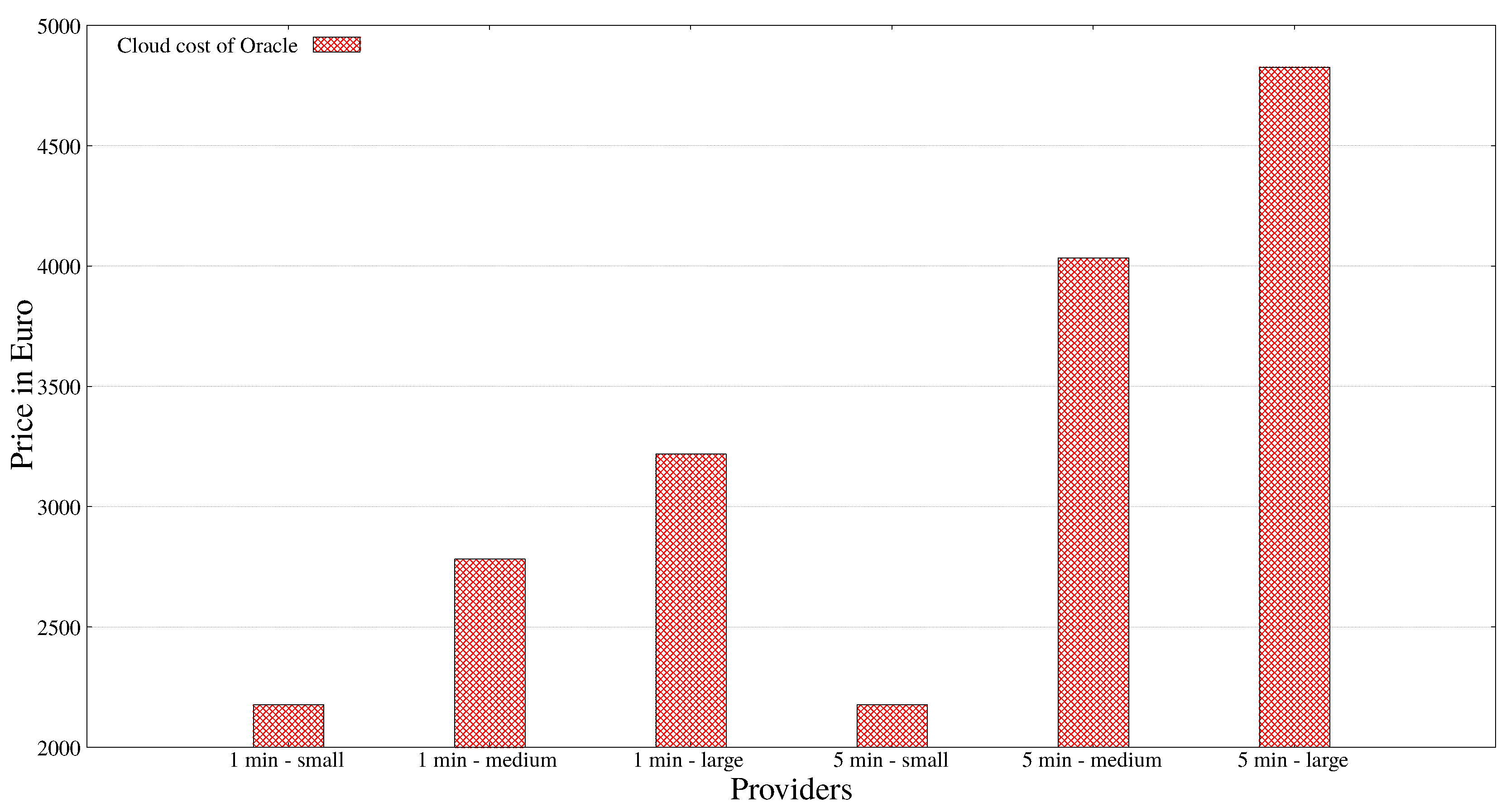
Figure 17.
Number of tasks and virtual machines in scenario N
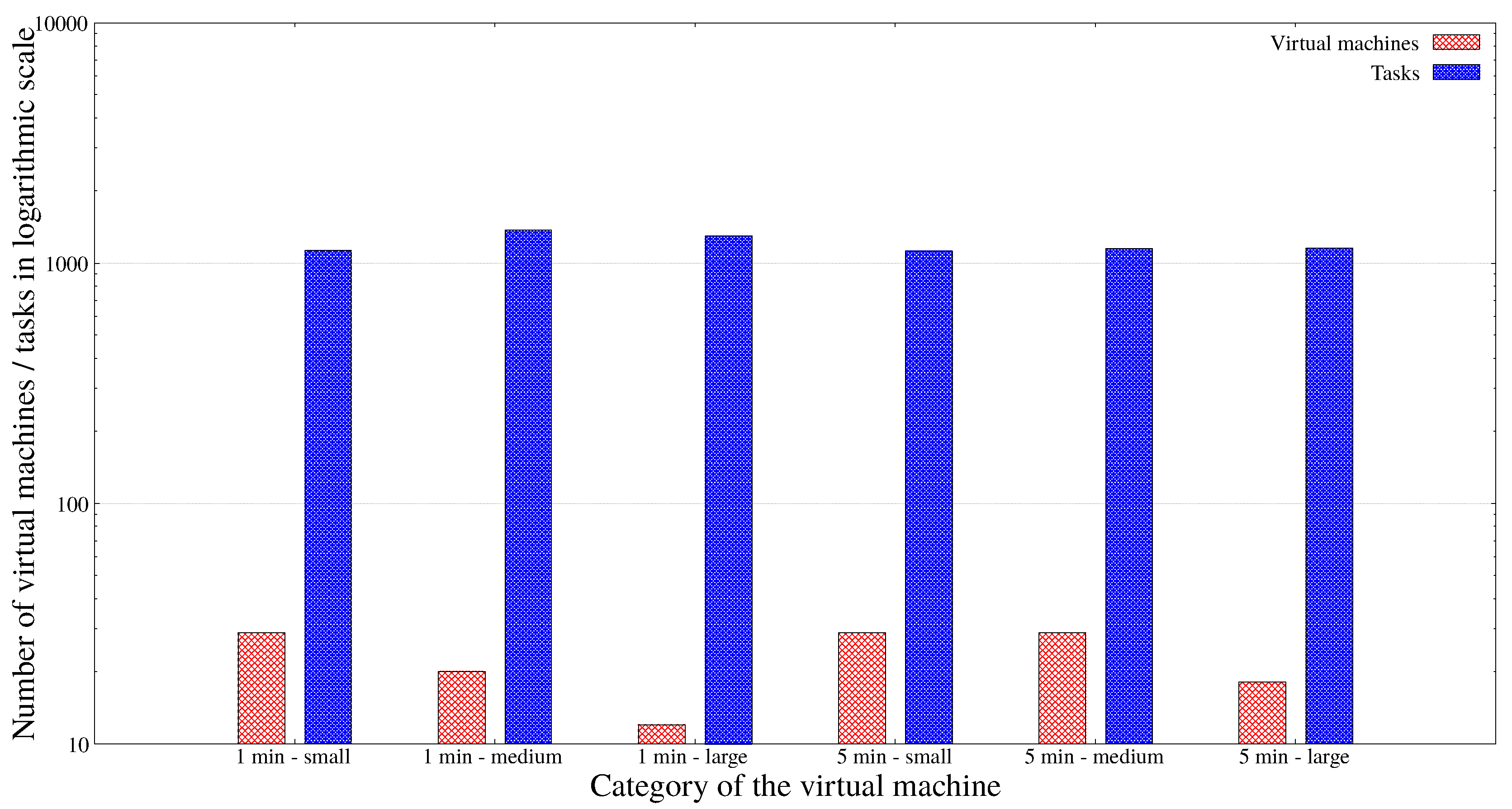
Figure 18.
Results of scenario N

Table 1.
Used VMs, number of task and produced data in scenario N
| Amount of Data (Byte) | Number of VMs | Number of Tasks | Produced Data (GB) |
|---|---|---|---|
| 50 | 12 | 1153 | 0.261 |
| 100 | 27 | 2299 | 0.522 |
| 200 | 28 | 4486 | 1.044 |
Table 2.
Used Virtual Machines (VMs), number of tasks and produced data in scenario N
| Station Type | Number of VMs | Number of Tasks | Produced Data (GB) |
|---|---|---|---|
| fixed | 28 | 1555 | 0.348 |
| random | 28 | 1561 | 0.352 |
Table 3.
IoT costs with a small VM category in scenario N
| VM Category | Small | |||||||
|---|---|---|---|---|---|---|---|---|
| Interval | 1 min | 5 min | ||||||
| Azure cloud cost | 20.039 | 4.200 | ||||||
| IoT provider | Bluemix | Amazon | Oracle | Azure | Bluemix | Amazon | Oracle | Azure |
| IoT side cost | 0.31948 | 32.80 | 4464.00 | 4215.5 | 0.06371 | 6.5436 | 4464.00 | 4215.5 |
| Sum | 20.35848 | 52.839 | 4484.039 | 4235.539 | 4.26371 | 10.7436 | 4468.2 | 4219.7 |
Table 4.
IoT costs with a medium VM category in scenario N
| VM Category | Medium | |||||||
|---|---|---|---|---|---|---|---|---|
| Interval | 1 min | 5 min | ||||||
| Azure cloud cost | 32.538 | 5.45 | ||||||
| IoT provider | Bluemix | Amazon | Oracle | Azure | Bluemix | Amazon | Oracle | Azure |
| IoT side cost | 0.31948 | 32.80 | 4464.00 | 4215.5 | 0.06371 | 6.5436 | 4464.00 | 4215.5 |
| Sum | 32.85748 | 65.338 | 4496.538 | 4248.038 | 5.51371 | 11.9936 | 4469.45 | 4220.95 |
Table 5.
IoT costs with a large VM category in scenario N
| VM Category | Large | |||||||
|---|---|---|---|---|---|---|---|---|
| Interval | 1 min | 5 min | ||||||
| Azure cloud cost | 62.667 | 7.128 | ||||||
| IoT provider | Bluemix | Amazon | Oracle | Azure | Bluemix | Amazon | Oracle | Azure |
| IoT side cost | 0.31948 | 32.80 | 4464.00 | 4215.5 | 0.06371 | 6.5436 | 4464.00 | 4215.5 |
| Sum | 62.98648 | 95.467 | 4526.667 | 4278.167 | 7.19171 | 13.6716 | 4471.128 | 4222.628 |
Table 6.
Cloud and IoT costs in scenario N
| IoT Provider | Bluemix | Amazon | Oracle | Azure | ||||
|---|---|---|---|---|---|---|---|---|
| IoT side cost | 0.18 | 18.92 | 14136.00 | 421.65 | ||||
| VM function | ON | OFF | ON | OFF | ON | OFF | ON | OFF |
| Bluemix cloud cost | 51.80 | 89.39 | 51.80 | 89.39 | 51.80 | 89.39 | 51.80 | 89.39 |
| Sum | 51.98 | 89.58 | 70.72 | 108.31 | 14187.80 | 14225.39 | 473.45 | 511.04 |
© 2017 by the authors. Licensee MDPI, Basel, Switzerland. This article is an open access article distributed under the terms and conditions of the Creative Commons Attribution (CC BY) license (http://creativecommons.org/licenses/by/4.0/).
Share and Cite
MDPI and ACS Style
Markus, A.; Kertesz, A.; Kecskemeti, G. Cost-Aware IoT Extension of DISSECT-CF. Future Internet 2017, 9, 47. https://doi.org/10.3390/fi9030047
AMA Style
Markus A, Kertesz A, Kecskemeti G. Cost-Aware IoT Extension of DISSECT-CF. Future Internet. 2017; 9(3):47. https://doi.org/10.3390/fi9030047
Chicago/Turabian StyleMarkus, Andras, Attila Kertesz, and Gabor Kecskemeti. 2017. "Cost-Aware IoT Extension of DISSECT-CF" Future Internet 9, no. 3: 47. https://doi.org/10.3390/fi9030047
Note that from the first issue of 2016, this journal uses article numbers instead of page numbers. See further details here.