Flow Shop Scheduling Problem and Solution in Cooperative Robotics—Case-Study: One Cobot in Cooperation with One Worker


1
Department of Visual Assistance Technologies, Fraunhofer Institute for Computer Graphic Research IGD, 18059 Rostock, Germany
2
Institute of Computer Science, University of Rostock, 18059 Rostock, Germany
*
Author to whom correspondence should be addressed.
Future Internet 2017, 9(3), 48; https://doi.org/10.3390/fi9030048
Submission received: 14 July 2017
/
Revised: 1 August 2017
/
Accepted: 11 August 2017
/
Published: 16 August 2017
Abstract
:This research combines between two different manufacturing concepts. On the one hand, flow shop scheduling is a well-known problem in production systems. The problem appears when a group of jobs shares the same processing sequence on two or more machines sequentially. Flow shop scheduling tries to find the appropriate solution to optimize the sequence order of this group of jobs over the existing machines. The goal of flow shop scheduling is to obtain the continuity of the flow of the jobs over the machines. This can be obtained by minimizing the delays between two consequent jobs, therefore the overall makespan can be minimized. On the other hand, collaborative robotics is a relatively recent approach in production where a collaborative robot (cobot) is capable of a close proximity cooperation with the human worker to increase the manufacturing agility and flexibility. The simplest case-study of a collaborative workcell is one cobot in cooperation with one worker. This collaborative workcell can be seen as a special case of the shop flow scheduling problem, where the required time from the worker to perform a specific job is unknown and variable. Therefore, during this research, we implement an intelligent control solution which can optimize the flow shop scheduling problem over the previously mentioned case-study.
1. Introduction and Related Research
Collaborative robotics is a novel successful trend in manufacturing which involves a safe cobot. The idea of the collaborative robotics is to gather the advantages of the industrial robot and the human worker together in the same work environment [1]. Since the manufacturing system is a matter of a continuous fluctuation in production demands such as the customization level and quantity [2], the presence of the human worker can be considered a very big advantage. This advantage stems from the fact that the worker can use his natural senses intuitively to form very complicated yet instant solutions. In contrast, the robot needs to be preprogramed to solve a specific problem.
A very simple example can be seen in an assembly scenario where the production customization level and volume is changing all the time. The worker can easily adapt his performance to assemble a new customized product without the need to stop the production process. Yet the cobot would be so useful if it could pick and place the exact needed parts of this customized product to the worker. The cobot can easily adapt to the pick and place operations based on previously programmed positions of all the product parts. In other words, it is much easier for the worker to adapt to manufacturing operations which require human experience such as assembly. While it is much more efficient for a cobot to adapt to much simpler operations such as pick and place. The efficiency of the cobot stems from the fact that it is more reliable than the worker in performing tasks that require heavy weight lifting or speed.
Sadik, and Urban are addressing the problem of self-organization in the cooperative workcell in [3]. They are mainly answering the question of how the cooperative workcell can continuously adapt to the variation in the number of workers or cobots during the cooperative manufacturing. The researchers are offering an interesting approach by combining the privileges of both the Holonic Control Architecture (HCA) and the International Society of Automation (ISA)-95 standard. The article applies the solution over a case-study which starts with two cobots in coordination with two workers. Then the number of the cobots varies from two to one and then to two again, the same variation in the worker numbers occurs as well. The results of the article show that the proposed solution is capable of achieving the maximum utilization of the available operational resources. Two important comments can be stated regarding this work, the first comment is that the researchers have used the event oriented concept to deal with the variation in the required time needed from the worker to accomplish an assigned task. In other words, the time needed from the worker to perform a task has never been measured or recorded during the presented case-study. The second comment is that they have only used the First Come First Serve (FCFS) method to schedule the cooperative tasks. Therefore, they did not test the effect of other scheduling methods on the production efficiency.
The research in [4] focuses on the cooperative workcell layout design and it extends that focus by proposing the question of how to allocate tasks among the existing cobots and workers. The research introduces an interesting investigation of the previous solutions to design a layout for a reconfigurable workcell. The article proposed an offline visualization tool to assist in task planning based on maximizing a utilization formula. One of the parameters which has been taken into consideration during task planning is the task completion time of the worker. It is not clear how this completion time has been obtained during the article, but it seems to be assumed in advance before deploying the simulation. If so, this makes the solution approach a bit shaky. Two case-studies have been used to test the research approach. During the two cases, the number of the cooperative resources is always fixed. That means that each time the number of the resources changes, the simulation should be rebuilt and redeployed again. In other words, the research does not put into consideration the adaption to the fluctuation in the number of the operational resources as a new dimension of configurability in the cooperative workcell. Moreover, the main motive of the research is to distribute the tasks among the available operational resources, and it does not schedule the whole existing group of tasks in the cooperative workcell.
The research in [5] addresses the physical safety problem in a cooperative workcell, the research introduces a novel approach to achieve the safety during the worker-industrial robot cooperation. The solution methodology suggested to estimate the worker task execution time. This estimation was based on an offline analysis of the worker and the industrial robot tasks in a simulation environment. From this analysis, the researchers were able to calculate the safety zone where the industrial robot is permitted to move. From a theoretical point of view, the research approach is well-explained. However, from the technical point of view, the article does not provide enough details to explain how to implement the solution over a real industrial case scenario. In our research, we address the scheduling problem which is another different subject than the physical safety in a cooperative robot. However, the idea of analyzing the worker task execution time in a cooperative manufacturing scenario seems to be not only useful for scheduling, but also for the physical safety.
In Section 2 of this article, we are going to explain the research case-study and formulate the research questions. In Section 3, we are going to introduce the research fundamentals which are needed to implement the solution. Section 4 will describe the solution implementation over the previously mentioned case-study. Finally, Section 5 will summarize and discuss the research to derive the conclusion and the future work.
2. Case-Study Description and Problem Formulation
The previous section has mentioned a practical example of a collaborative workcell, where one cobot is in cooperation with one worker in a reconfigurable manufacturing scenario. The cobot is responsible for the pick and place operations while the worker assembles the handled products. Due to the speed difference between the worker and the cobot, a buffer space is needed beside the worker to store the loaded jobs by the cobot till the worker is free to process them. In this paper, we will take this example as a case-study to show the solution approach.
In this case-study the production volume is continuously varying which leads to the fluctuation in the required time from both the cobot and the worker to complete a job. The required time from the cobot to pick and place the parts of an assigned job is unknown, however it can be calculated. Since the cobot speed is reliable, thus we can assume that the required time from the cobot to pick and place one job is a constant and equals to a Robot Time Constant (RTC). Therefore, by multiplying RTC by the required units number, the overall time can be calculated. On the other hand, the required time which is needed from the worker to assemble a job is varying, therefore this time cannot be calculated. However, it can be predicated by recording the needed time from the worker to assemble the previous jobs, then calculating the Worker Mean Time Value (WMTV), which can be used later to predict the overall needed time for assembling the next jobs.
The research question is very easy to state, yet it is very hard to answer. When a cobot is in coordination with a worker in the mentioned case-study. How can the control solution assign the next production job among many standing jobs to the cobot and the worker to minimize the overall makespan. Taking into consideration the previously mentioned uncertainty in the required time from the worker to accomplish a production job. The difficulty of answering this question stands from the fact that the answer is beyond an efficient scheduling algorithm only, since it needs an intelligent information control and communication solution which can understand the overall status of the workcell and monitor the worker time to be able to take logical decisions and therefore can apply the scheduling algorithm. During this research, we extend the research in [3] by applying Johnson algorithm to schedule the cooperation at the case-study. The required solution components as well as Johnson algorithm are going to be explained in details in the next section.
3. Solution Fundamentals
3.1. Johnson Algorithm for Two Stage Flow Shop Scheduling
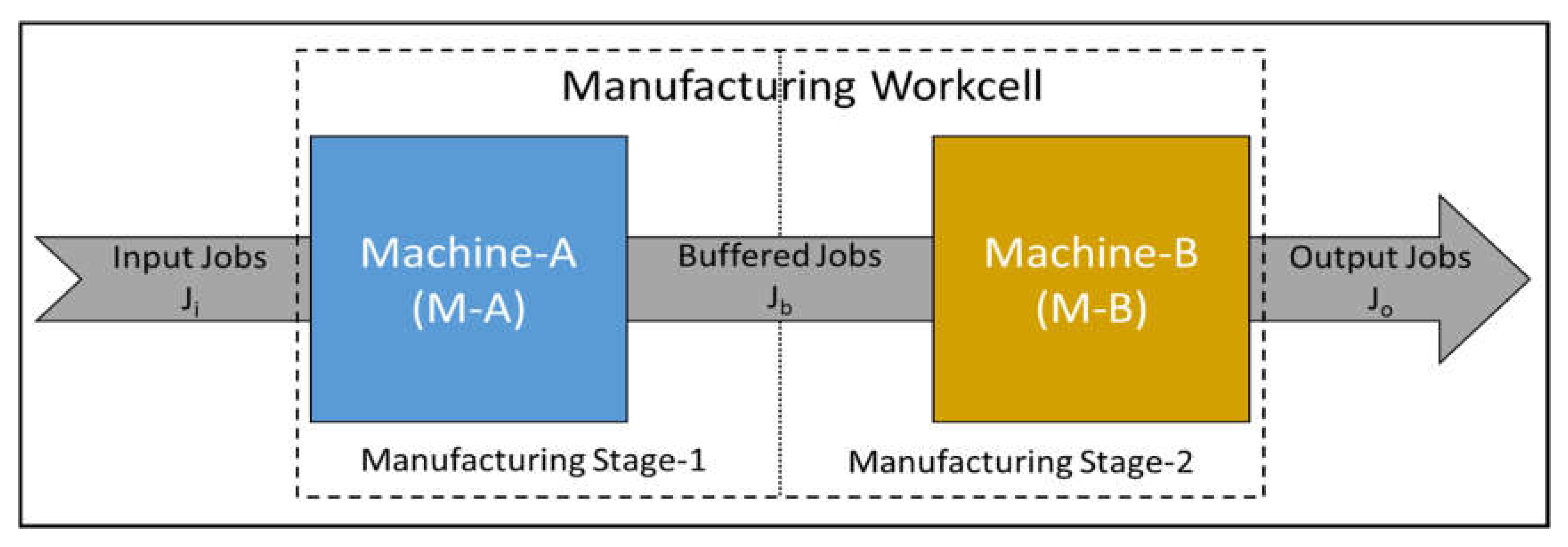
A typical two sequential stages flow shop scheduling problem can be solved by Johnson algorithm [6,7], Johnson scheduling model can be seen in Figure 1. The preconditions of this scheduling problem are that the production jobs always need to be processed by M-A first, then processed by M-B. The production speeds of M-A and B are different. Therefore, a buffer unit has to exist between M-A and B to recover this speed difference. Two kinds of time delay can be found, the first kind is M-B starvation delay, this means that M-B is free but waiting M-A to finish the current job to be able to start processing the same job. This delay must happen at least once at the first job assignment. The second kind of the time delay is the buffer delay. This delay happens when M-A has finished a job (Ji) while M-B is busy in processing a prior job. Therefore, Ji has to wait in the buffer till M-B is free and Ji processing turn comes.
Johnson algorithm tries to minimize the previously mentioned delays. Therefore, it minimizes the makespan of M-B which is the longest makespan of that manufacturing workcell [8]. Jonson algorithm can be summarized by the next three steps:
- Step-1: Find the shortest processing time among all the present non-scheduled standing jobs. If two or more jobs have the same processing time. Select one of them arbitrarily.
- Step-2: If the shortest processing time locates on M-A, schedule the corresponding job as the soonest. If the shortest processing time locates on M-B, schedule the corresponding job as the latest.
- Step-3: Eliminate the job that has been scheduled from the present non-scheduled standing jobs. Repeat steps 1 and 2 till scheduling all the jobs.
The left section of Table 1 shows a group of unscheduled jobs Ji. In order to schedule those jobs using Johnson algorithm we should find the shortest Processing Time (TP) which is J1 and equals to 5 time units, since this time locates on M-B, therefore it has to be scheduled at the end of the queue. J2 comes after with the shortest TP on M-A, therefore it has to be scheduled at the beginning of the queue. Then J5 is the job with the shortest TP on M-B, therefore we put it before J1. Finally, we find that J3 and J4 are equal in the shortest TP on M-A, therefore we select one of them arbitrarily to come after J2. In this example, we selected J4 to be scheduled first then J3. In order to prove that Johnson scheduling is the optimum solution, we compared it with the FCFS scheduling method which can also be seen at the middle section of Table 1 and in Figure 2a. By calculating the Operation Time (TO) based on the given TP. We can see that the makespan of the FCFS scheduling is 54 time units. While, by applying Johnson algorithm, the makespan is reduced to 49 time units which can be seen at the right section of Table 1 and in Figure 2b.
3.2. Holonic Control Architecture and Artificial Agents
HCA is a distributed control solution architecture which has been frequently used to solve the problem of reconfigurable manufacturing system [9,10]. The HCA defines the holon as an autonomous and cooperative building unit of the manufacturing system, the holon is mainly responsible for transforming, transporting, storing, and validating the information and the physical inputs. The HCA divides the manufacturing process tasks and responsibilities over different holon categories. The most known HCA model is the Product-Resource-Order-Staff-Architecture (PROSA), which is shown in Figure 3a. The PROSA basic holons are:
- Product Holon (PH): is responsible for processing and storing the different production plans which are necessary to obtain the proper manufacturing of a certain product.
- Order Holon (OH): is responsible for composing, managing the production orders. Furthermore, in a small scale enterprise, the OH distribute the tasks assignment among the existing operating resources and hence it monitors the execution of these assigned tasks.
- Operational Resource Holon (ORH): an entity on the shop floor which represents a physical object such as a machine, a robot, or a worker.
The most common technology to apply the HCA concept is the software agent. An artificial agent is a piece of code which is deployed in a particular environment and is able to accomplish autonomous actions in this environment to achieve some criteria which are specified by the artificial agent programmer [11]. An agent is autonomous by nature. The meaning of agent autonomy is that the agent self-steers its actions without direct assistance of the humans, and has a high degree of a self-directed control over its actions and its internal states. To achieve the concept of autonomy, the agent must be responsive, pro-active, and social. ‘Responsive’ means that the agent can perceive its environment and respond as fast as it is needed to the different changes happen in this environment. ‘Pro-active’ means that the agent is capable of taking initiatives based on a set of goal directed behaviors, thus it can exhibit opportunistic behavior. Finally, ‘social’ means that the agent can solve the problems and reach its goals by being able to interact with other autonomous agents and humans in its environment [12].
Conceptually, an autonomous agent is an artificial software problem solver [13]. This means that the autonomous agent must be able to select a specific set of actions and build its own plans to solve an existing problem. The set of actions which are selected to be executed by an autonomous agent is called a behavior. The artificial agent behaviors are coded by the agent developer. One or more behaviors can execute by an artificial agent to achieve its goal. The choice of a specific behavior among many should be based on a proper criterion which has been developed by the agent software creator. The agent socialization is the method that an agent would use to collect the information from its environment, therefore it can build an execution plan. A Multi-Agent System (MAS) is a flexible topology which links a group of artificial agents. The idea of the MAS is to compose a team of artificial agents whom together can solve a problem beyond the capabilities of an individual artificial agent [14].
The most famous middleware to apply the autonomous agent concept is JAVA Agent Development Environment (JADE) [15], which can be seen in Figure 3b. An instance of JADE runtime is an independent thread over a specific operating system. This instance is composed of a set of containers. A container by definition is a group of autonomous agents which are deployed under the same instance of JADE runtime. Every JADE runtime must have at least a main container, which contains two substantial agents. Those two substantial agents are the Agent Management System (AMS) and the Directory Facilitator (DF). AMS is responsible for giving a unique agent ID (AID) for every agent under its platform. The AID is mainly used as the communication address for an agent. Meanwhile, the DF is the yellow pages of JADE. This means that DF knows the services which can be provided by all the agent under a JADE runtime. Therefore, it can announce those services to obtain the service oriented communication policies [16]. JADE applies a standard communication protocol which is founded by the Foundation for Intelligent Physical Agent (FIPA) specifications. FIPA is an IEEE Computer Society standard which supports the creation of an agent-based network and guarantees interoperability with the other available standard technologies [17]. JADE agents use FIPA-Agent Communication Language (FIPA-ACL) in order to exchange the ACL-messages either inside or outside its operating platform. Furthermore, JADE provides a Graphical User Interface (GUI) to help the agent programmer to develop, deploy, and debug a MAS [18].
3.3. Rule Management System and Drools
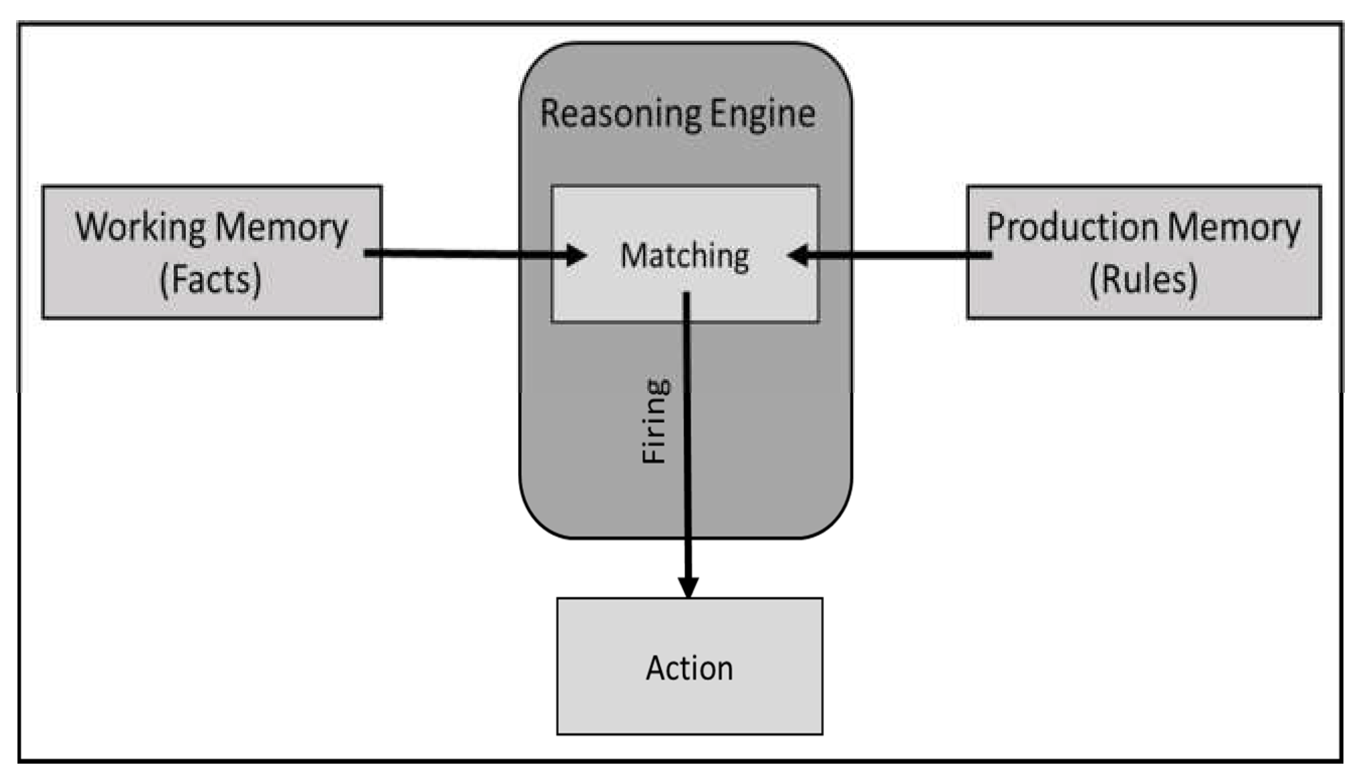
A Rule Management System (RMS) is a form of an expert system which usually uses an ontology based representation to codify the information into a knowledge base that can be used for reasoning [19]. An RMS depends on two kind of memory as it is shown in Figure 4. The working memory holds the facts which present the domain knowledge, while the production memory holds a set of rules which are usually presented in a form of conditional statements. The reasoning engine solves a given problem by matching the present facts with the existing rules. The reasoning engine organizes and controls the follow of the solution route based on one of the following reasoning methods [20]:
- Forward reasoning chaining: in forward reasoning chaining, the RMS starts with a set of initial facts then it determines new facts every time a rule matches a fact. The RMS will go through a chain of rules firing sessions to reach its final target, which ultimately leads to find the solution route from the initial facts to the final goal in a forward approach of reasoning.
- Backward reasoning chaining: in backward reasoning chaining, the RMS starts from the final goal, then it finds which rules must be fired to lead to this goal, therefore the RMS can determine the facts which are needed to reach the final goal. During the backward chaining, a consequence of sub-goals will appear, which ultimately leads to find the solution route from the final goal to the initial sub-goal in a backward approach of reasoning.
Drools is a Business Rule Management System (BRMS) that has been created by jboss organization, therefore it adds more features than a regular RMS [21]. As it provides a tool for a rule-based solution creation, managing, deploying, and analyzing. One of the biggest advantages of Drools is its ability to apply a hybrid chaining reasoning. A hybrid chaining reasoning is a mix between the forward and the backward chaining which can be more efficient in some cases than both. Also, Drools extends the Rete algorithm for pattern matching which called ReteOO. ReteOO denotes the enhancement of Rete algorithm by combing it with other Object Oriented (OO) concepts such as abstraction, inheritance, and encapsulation.
4. Solution Implementation
4.1. Johnson Algorithm for Two Stages Flow Shop Scheduling
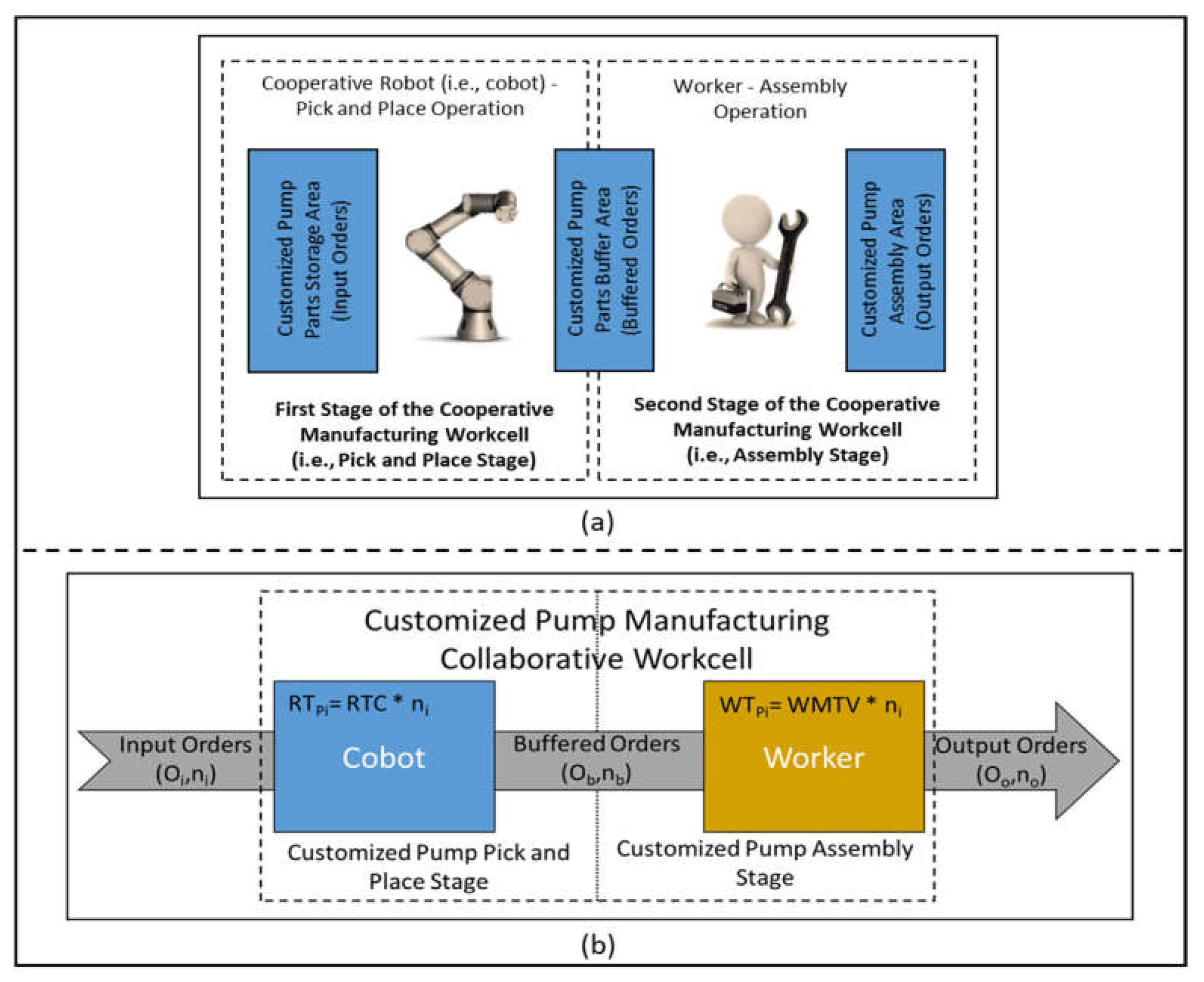
Figure 5 shows the shop flow model of the previously mentioned case-study. The model is a special case of the two sequential stages manufacturing workcell which has been described in detail in Section 3.1. A set of jobs (Oi, ni) is assumed to be picked and placed by the cobot, where Oi denotes the customized pump order in the same sequence they have been received and ni denotes the required number of units of this order. In the context of reconfigurable manufacturing, the production order is a customized version of a specific product. In our case-study a centrifugal pump (CP) manufacturing has been chosen as an example for a reconfigurable product. At the first stage of the cooperative workcell, it has been assumed that the cobot will always take the same time constant (RTC) to pick and place any pump regardless the customization level. Therefore, the required TP from the cobot to pick and place a customized order (RTPi) equals to the RTC multiplied by ni. At the second stage of the cooperative workcell, it has been assumed that we can continuously record the required time from the worker to assemble a job (Oi, ni). Thus, an average time value (WMTV) can be calculated. Therefore, a predication for the required processing time from the worker to assemble the next job (WTP(i+1)) can be estimated as WMTV multiplied by ni+1. An example of calculating the job processing time can be seen in Table 2.
Johnson algorithm is mainly depending on finding the shortest job processing time. This makes the algorithm simpler due to the assumption in our case-study. This is because RTPi and WTPi are correlated to each other’s by ni, while this correlation did not exist at Table 1. Therefore, Johnson algorithm can be obtained by comparing RTC to WMTV as shown in Table 2. Let us assume that n1 is less than n2. In case one, we will assume that RTC is less than or equal to WMTV, this means that RTP1 must be the shortest unscheduled processing time. Therefore, the sequence of the scheduled jobs will be J1 then J2. In case two, we will assume that RTC is greater than or equal to WMTV, this means that WTP1 must be the shortest unscheduled processing time. Therefore, the sequence of the scheduled jobs will be J2 then J1. From this comparison, we can modify Johnson steps to schedule the jobs based on the ascending sequence of ni, if RTC is less than or equal to WMTV. Otherwise, scheduling of the jobs is based on the descending sequence of ni.
4.2. Holonic Control Architecture Implementation
Figure 6 shows the GUI for the implemented case-study. While Figure 7 shows the interaction and the behaviors of those holons. Four holons exist in this implementation. The first holon is the PH with a GUI shown in Figure 6a. The PH is generating the pump order by choosing the pump size and quantity. By pressing send order button, the product agent which is shown in Figure 7a triggers a one shot behavior which sends the job via an ACL-message to the OH. The ACL-message contains the job details and it has an AGREE communication act as can be seen in Figure 6b. The OH GUI is shown in Figure 6b. The order agent implements a cyclic behavior which continuously receives the jobs from the pump agent. The AGREE-message sending/receiving operation is shown in line-1 of Figure 7b.
When the order agent receives a new job, it fires a new Drools reasoning session. The reasoning engine will perform a FCFS or Johnson scheduling based on the overall status of the cooperative workcell. The rules that control the scheduling decision making can be seen in details in Table 3. IF the cobot is free, the scheduled pump job will be assigned to it as it can be seen via the Robot Holon (RH) GUI in Figure 6c. A one shot behavior is triggered by Drools reasoning engine to send a REQUST-message to the robot agent as it can be seen in line 2 of Figure 7b. The robot agent has a cyclic behavior which continuously receives the job assignments.
When the robot agent receives a new job assignment, it initializes a timer with a value of ni multiplied by RTC. In our case-study we assumed that RTC value equals to 2.0 s. When the timer is elapses, the robot agent sends an INFORM message to the order agent to inform it has picked and placed the assigned task. This INFORM-message can be seen in line 3 of Figure 7b. When the order agent receives a robot done event, it fires a new Drools reasoning session. Drools will reschedule the existing standing jobs due to the decision table rules. Moreover, IF the worker is free, the scheduled jobs will be assigned to the worker as it can be seen via the Worker Holon (WH) GUI in Figure 6d.
A one shot behavior is triggered by the Drools reasoning engine to send a REQUST-WHEN-message to the worker agent as it can be seen in line 4 of Figure 7b. The worker agent has a cyclic behavior which is continuously receiving the order assignments. When the worker finishes assembling all the pump orders, he presses a task done button via his GUI. By pressing the worker task done, the worker agent triggers a one shot behavior which sends an INFORM-IF-message to the order agent. The INFORM-IF-message can be seen in line 5 of Figure 7b. When the order agent receives a worker done event, it fires a new Drools reasoning session. Drools will calculate the WMTV every time the OH receives a worker done event. Therefore, the rest of the scheduling will be based on the current WMTV.
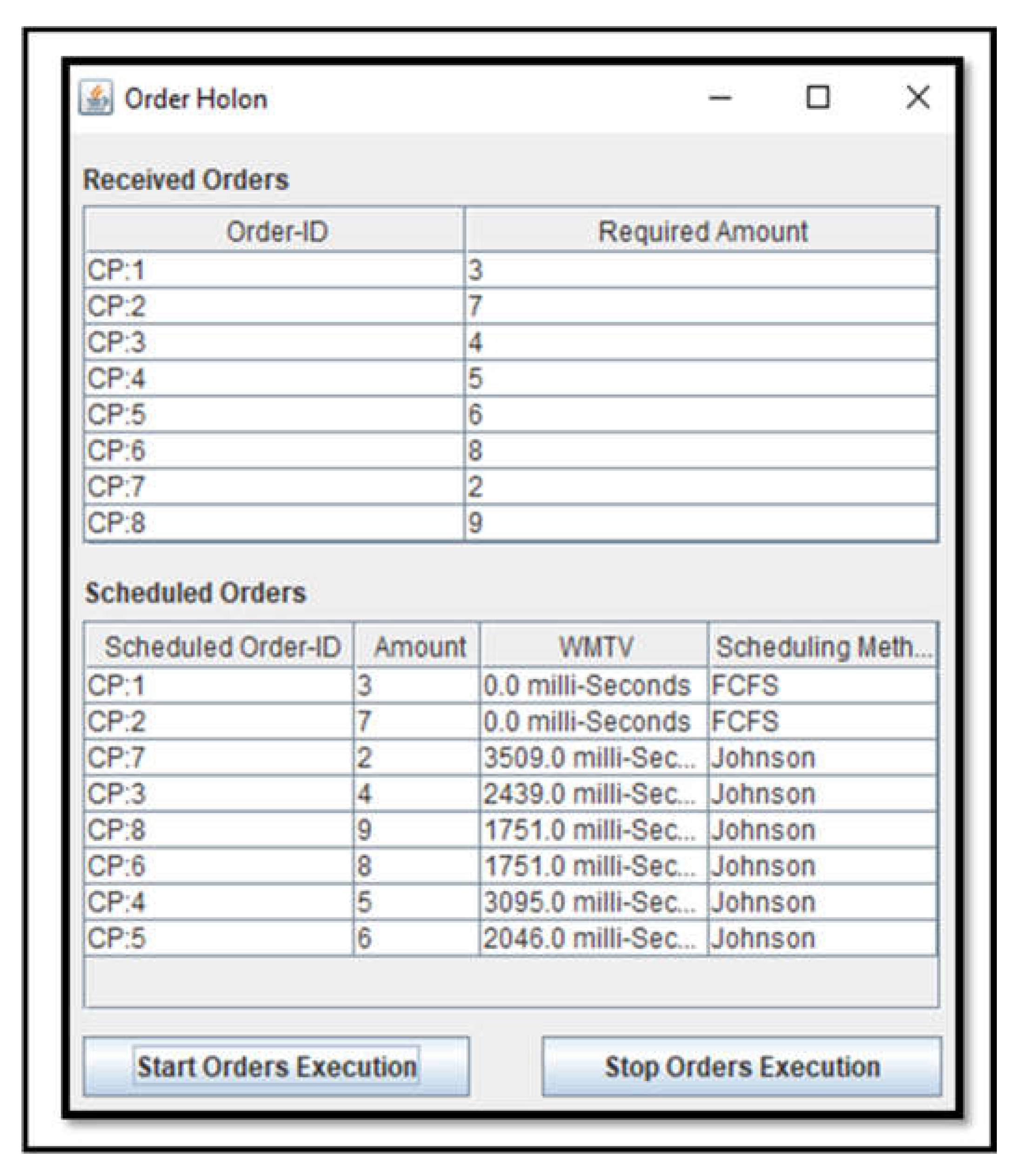
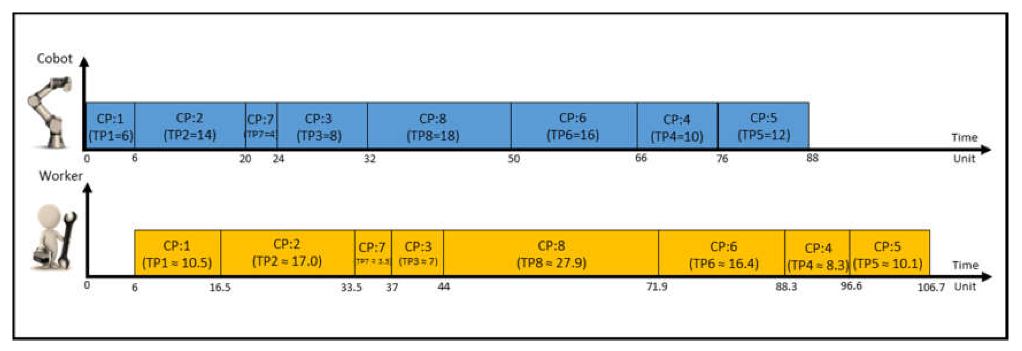
Figure 8 and Figure 9 show the scheduling results due to the calculation of the WMTV and the decision rules which are well-explained in Table 3. There are eight received jobs in Figure 8 which start with order-ID (CP:1) and end with order-ID (CP:8). Every pump order has a different customization level and a specific required quantity. However, the pump customization is out of the focus of this article (refer to [3]). The jobs scheduling is based on the previously mentioned Johnson algorithm for our case-study. By starting the production execution, the first two jobs (CP:1, CP:2) are scheduled based on FCFS. The reason behind selecting FCFS as a scheduling method is that the worker had not finished assembling CP:1 till CP:2 has been scheduled.
When the cobot finished to handle CP:2, the worker was already done with CP:1, therefore the value of WMTV could be calculated as 3.5 s which is greater than the value of RTC (i.e., 2.0 s). Therefore, the OH started to schedule the remaining jobs based on ascending their required quantity, that is why CP:7 (i.e., the least unscheduled quantity) was scheduled as the earliest. When the cobot has done with handling CP:7, the value of WMTV was 2.4 s which is still greater than the value of RTC. Therefore, the OH kept the scheduling based on ascending the required quantity, that is why CP:3 was scheduled as the earliest.
When the cobot was done with handling CP:3, the value of WMTV was 1.7 s which is less than the value of RTC. Therefore, the OH started to schedule the jobs based on descending their required quantity, that is why CP:8 (i.e., the biggest unscheduled quantity) was scheduled as the earliest. When the cobot has done with CP:8, the value of WMTV was still the same as before, therefore the OH has kept the scheduling based on descending the required quantity, that is why CP:6 was scheduled as the earliest.
When the cobot has done with handling job CP:8, the value of WMTV was 3.09 s, which is greater than the value of RTC. Therefore, the OH started again to schedule the jobs based on ascending their required quantity, that is why CP:4 was scheduled as the earliest. When the cobot was done with handling CP:4, the value of WMTV was 2.04 s which is still greater than the value of RTC. Therefore, the OH kept the scheduling based on ascending values of the required quantity, that is why CP:5 has been scheduled as the final scheduled job.
5. Summary, Conclusions, and Future Work
During this article, we introduced the problem of scheduling the production tasks in case of one cobot in collaboration with one worker in a reconfigurable manufacturing scenario. Taking into consideration the fluctuation in the required production customization level and quantity, we derived the idea of collaboration. Since the cobot is reliable in terms of speed and weight lifting, it therefore can be assigned to simple operations to adapt to such as pick and place operations. Meanwhile, the worker can adapt to more complex operations such as assembly operations.
The article proposed a solution approach via an analogy between Johnson scheduling algorithm and the case-study scenario. The analogy was based on the assumption that the required time for the worker to finish a certain job can be always monitored and recorded, then that time value was used to predict the worker task time for the future jobs and compare it to the required time from the cobot the same future jobs. The HCA has been used to implement this solution via the autonomous reactive agent and the rule management system technologies. The OH was responsible for receiving the jobs from the PH, then scheduling them based on a comparison between RTC and WMTV. Ultimately, the OH can assign the jobs for the cobot and the worker based on their statuses. The OH used JADE agent messaging to comprehend the production jobs and the statuses of the cobot and the worker, and also to calculate the WMTV. Simultaneously, the OH used Drools RMS to take a scheduling or a job assignment decision.
The case-study implementation showed the success of the solution approach. That is because the solution optimized the two kinds of delay which can exit in two stage cooperative workcell. The first delay is a result of the worker starvation. This means that the worker is in free status but waiting for the cobot to process the job. This delay must happen at least one once at the very beginning of the case-study implementation. Otherwise, the worker was always busy during the rest of the implementation. The worker starving delay was minimized even when the WMTV was less than the RTC (i.e., the worker is faster than the cobot). The second source of delay which was optimized by the solution is the buffer delay. This delay can be so obvious when the cobot is done with handing all the scheduled jobs while the worker is still operating. To minimize this delay, the shortest jobs of the worker should be held to the end of the scheduling. However, the solution does not aim to only minimize that delay as it also tries to adapt to the current situation to optimize the two kinds of delay in the workcell. Therefore, we could see at the case-study implementation that the first two jobs have been scheduled as FCFS, then the solution started to schedule based on Johnson algorithm and the time has been taken from the worker to finish the previous jobs. Thus, when the cobot was done with handing all the scheduled jobs, the worker was done with the first scheduled five jobs and assembling the sixth job. This can be derived by counting the number of changes in the value of WMTV in Figure 8. This means that CP:4 and CP:5 were still in the buffer when the cobot was done with all the scheduled jobs. The sum of the required units in CP:4 and CP:5 is 11 units. This number was not the minimum quantity of the two jobs, but it was the optimal due to the previously explained scenario of the case-study.
During this research, we tried to simplify Johnson algorithm by using RTC, WMTV, and ni. The main reason behind that was to facilitate the illustration of the whole solution idea. However, the same solution approach can be accomplished by using the original steps of Johnson algorithm. This can fit other operations which have no specific number of units but still the time of the operation is variable. However, finding a correlation between the cobot and the worker processing times will always simplify Johnson scheduling steps. The same approach of measuring the worker time of executing a task can be used as well if the cobot task time is variable. Then predicting the next jobs processing time based on those measurements to achieve Johnson scheduling at the next job assignment. Even though the case-study was a very specific scenario, the same solution approach can be followed to extend the number of collaborated operational resources, or the nature of the manufacturing scenario. Therefore, in our future research, we will study more generic case-studies and add more collaborative resources to the study.
Acknowledgments
This research has been supported by the German Federal State of Macklenburg-Western Pomerania and the European Social Fund under grant ESF/IV-BM-B35-0006/12 and by grants from University of Rostock and Fraunhofer IGD.
Author Contributions
Ahmed R. Sadik conceived the implementation and the analysis of the case study and studied the interaction; Bodo Urban conceived the research concept and the problem statement.
Conflicts of Interest
The authors declare that there is no conflict of interest.
References
- Sadik, A.; Urban, B. A Holonic Control System Design for a Human & Industrial Robot Cooperative Workcell. In Proceedings of the 2016 International Conference on Autonomous Robot Systems and Competitions (ICARSC), Bragança, Portugal, 4–6 May 2016; pp. 118–123. [Google Scholar]
- Elmaraghy, H.A. Flexible and reconfigurable manufacturing systems paradigms. Int. J. Flex. Manuf. Syst. 2005, 17, 261–276. [Google Scholar] [CrossRef]
- Sadik, A.; Bodo, U. Combining Adaptive Holonic Control and ISA-95 Architectures to Self-Organize the Interaction in a Worker-Industrial Robot Cooperative Workcell. Future Internet 2017, 9, 35. [Google Scholar] [CrossRef]
- Tsarouchi, P.; Michalos, G.; Makris, S.; Athanasatos, T.; Dimoulas, K.; Chryssolouris, G. On a human–robot workplace design and task allocation system. Int. J. Comput. Integr. Manuf. 2017, 1–8. [Google Scholar] [CrossRef]
- Pellegrinelli, S.; Moro, F.; Pedrocchi, N.; Molinari Tosatti, L.; Tolio, T. A probabilistic approach to workspace sharing for human–robot cooperation in assembly tasks. CIRP Ann.-Manuf. Technol. 2016, 65, 57–60. [Google Scholar] [CrossRef]
- Stevenson, W.; Ness, P. Study Guide for Use with Production/Operations Management; McGraw-Hill: Boston, MA, USA, 1999. [Google Scholar]
- Grzechca, W. Manufacturing in Flow Shop and Assembly Line Structure. Int. J. Mater. Mech. Manuf. 2015, 4, 25–30. [Google Scholar] [CrossRef]
- Al-Harkan, I.M. On Merging Sequencing and Scheduling Theory with Genetic Algorithms to Solve Stochastic Job Shops. PH.D. Thesis, University of Oklahoma, Norman, OK, USA, 1997. [Google Scholar]
- Babiceanu, R.; Chen, F. Development and Applications of Holonic Manufacturing Systems: A Survey. J. Intell. Manuf. 2006, 17, 111–131. [Google Scholar] [CrossRef]
- Van Brussel, H.; Wyns, J.; Valckenaers, P.; Bongaerts, L.; Peeters, P. Reference architecture for holonic manufacturing systems: PROSA. Comput. Ind. 1998, 37, 255–274. [Google Scholar] [CrossRef]
- Botti, V.; Giret, A. Holonic Manufacturing Systems. In ANEMONA—A Multi-Agent Methodology for Holonic Manufacturing Systems, 1st ed.; Springer: London, UK, 2008; pp. 7–20. [Google Scholar]
- Jennings, N.; Wooldridge, M. Agent Technology, 1st ed.; Springer: Berlin, Germany, 1998; pp. 3–28. [Google Scholar]
- Shen, W.; Hao, Q.; Yoon, H.; Norrie, D. Applications of agent-based systems in intelligent manufacturing: An updated review. Adv. Eng. Inform. 2006, 20, 415–431. [Google Scholar] [CrossRef]
- De Meo, P.; Messina, F.; Rosaci, D.; Sarné, G. An agent-oriented, trust-aware approach to improve the QoS in dynamic grid federations. Concurr. Comput. Prac. Exp. 2015, 27, 5411–5435. [Google Scholar] [CrossRef]
- Jade Site. Available online: http://jade.tilab.com/ (accessed on 8 January 2017).
- Teahan, W. Artificial Intelligence–Agent Behavior, 1st ed.; BookBoon: London, UK, 2010. [Google Scholar]
- Bellifemine, F.; Caire, G.; Greenwood, D. Developing Multi-Agent Systems with JADE, 1st ed.; Wiley: Chichester, UK, 2008. [Google Scholar]
- FIPA Site. Available online: http://www.fipa.org/ (accessed on 1 February 2017).
- Ordóñez, A.; Eraso, L.; Ordóñez, H.; Merchan, L. Comparing Drools and Ontology Reasoning Approaches for Automated Monitoring in Telecommunication Processes. Procedia Comput. Sci. 2016, 95, 353–360. [Google Scholar] [CrossRef]
- Al-Ajlan, A. The Comparison between Forward and Backward Chaining. Int. J. Mach. Learn. Comput. 2015, 5, 106–113. [Google Scholar] [CrossRef]
- Drools Expert User Guide. Available online: https://docs.jboss.org/drools/release/5.2.0.CR1/drools-expert-docs/html_single/ (accessed on 18 April 2017).
Figure 1.
Model of two sequential stages manufacturing workcell.

Figure 2.
(a) First Come First Serve Scheduling Gantt chart; (b) Johnson Scheduling Gantt chart.
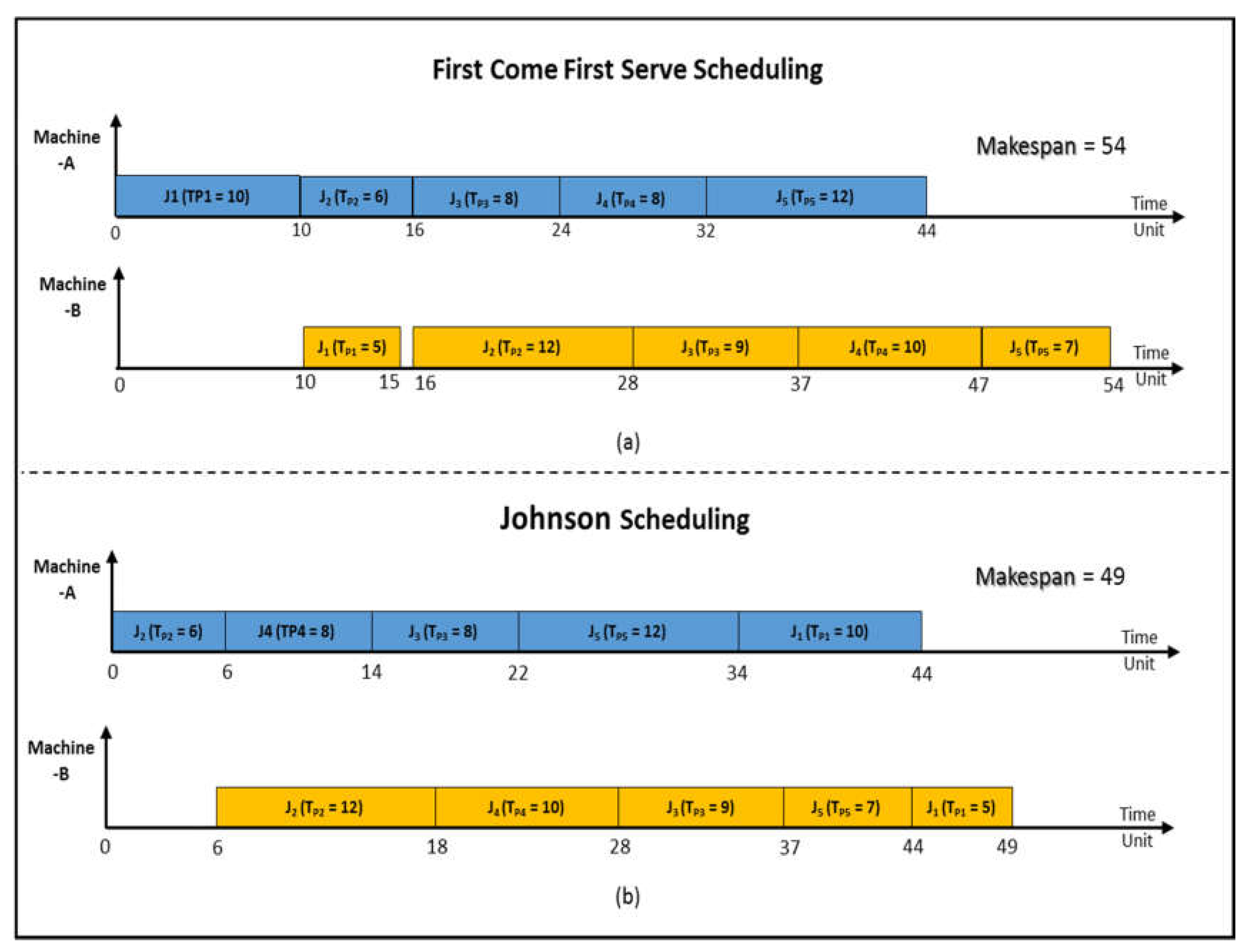
Figure 3.
(a) PROSA (Product-Resource-Order-Staff-Architecture) model; (b) JADE (JAVA Agent Development Environment) framework.
Figure 3.
(a) PROSA (Product-Resource-Order-Staff-Architecture) model; (b) JADE (JAVA Agent Development Environment) framework.
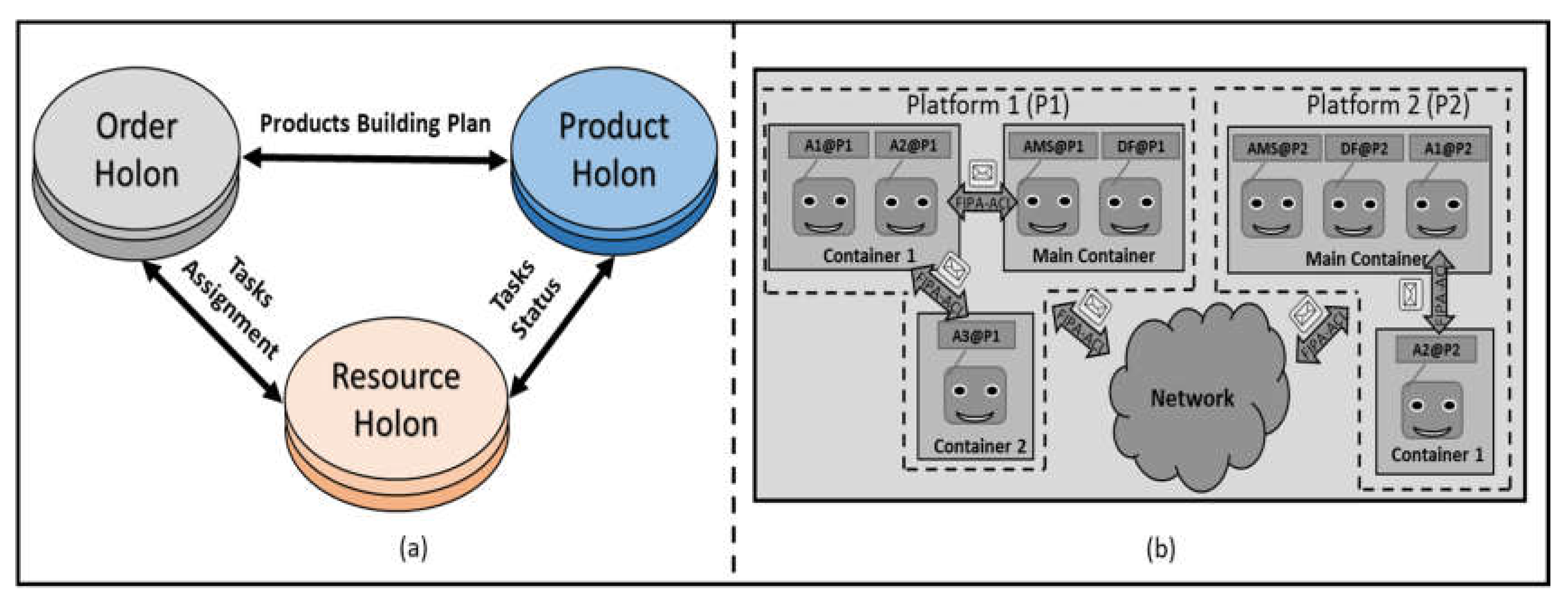
Figure 4.
Rule Management System components.

Figure 5.
(a) Model of the case-study workcell; (b) Analysis of the case-study model.

Figure 6.
(a) Product Holon Interface; (b) Order Holon Interface; (c) Robot Holon Interface; (d) Worker Holon Interface.
Figure 6.
(a) Product Holon Interface; (b) Order Holon Interface; (c) Robot Holon Interface; (d) Worker Holon Interface.
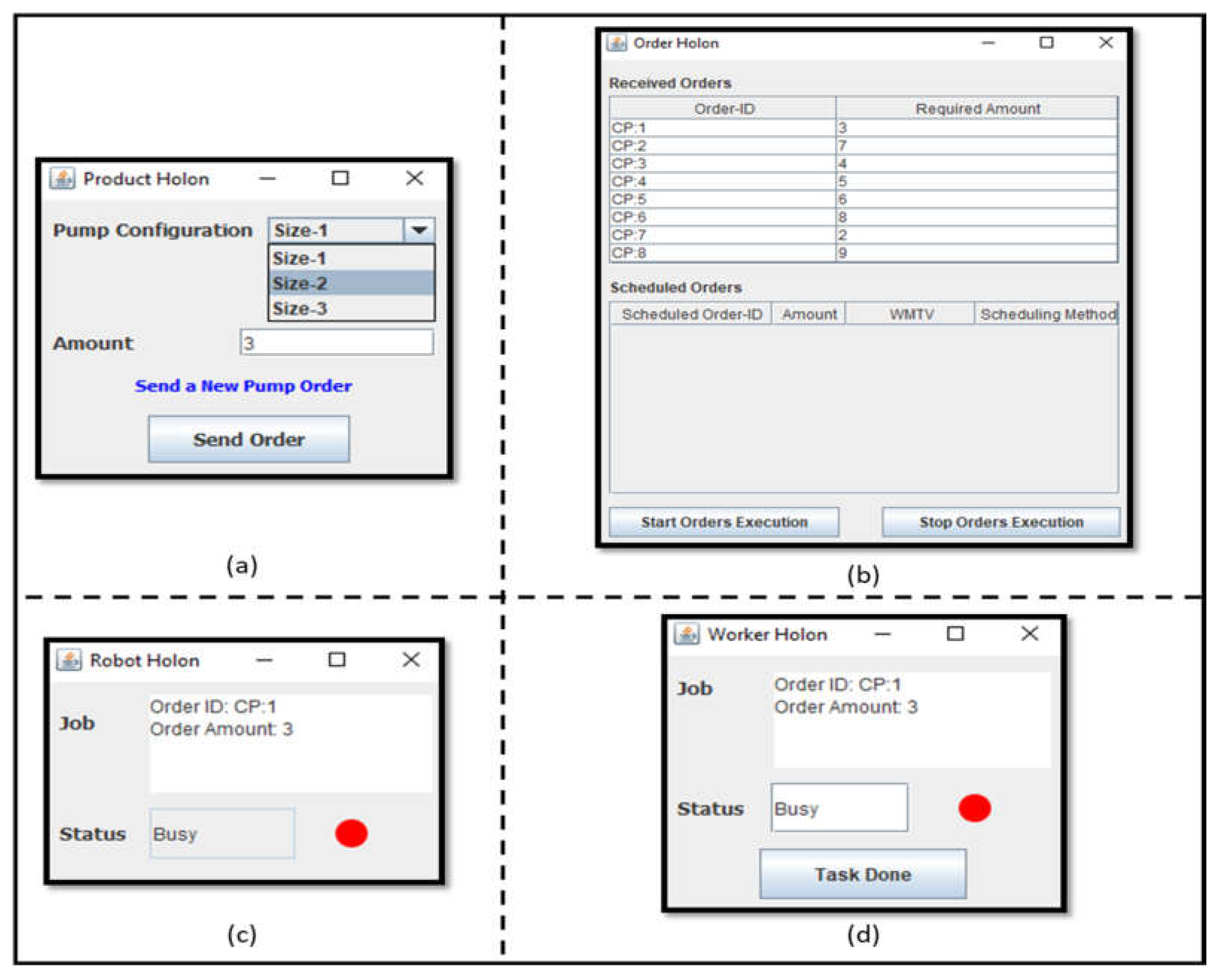
Figure 7.
(a) Case-study holons interaction and behaviors; (b) Case-study communication model.
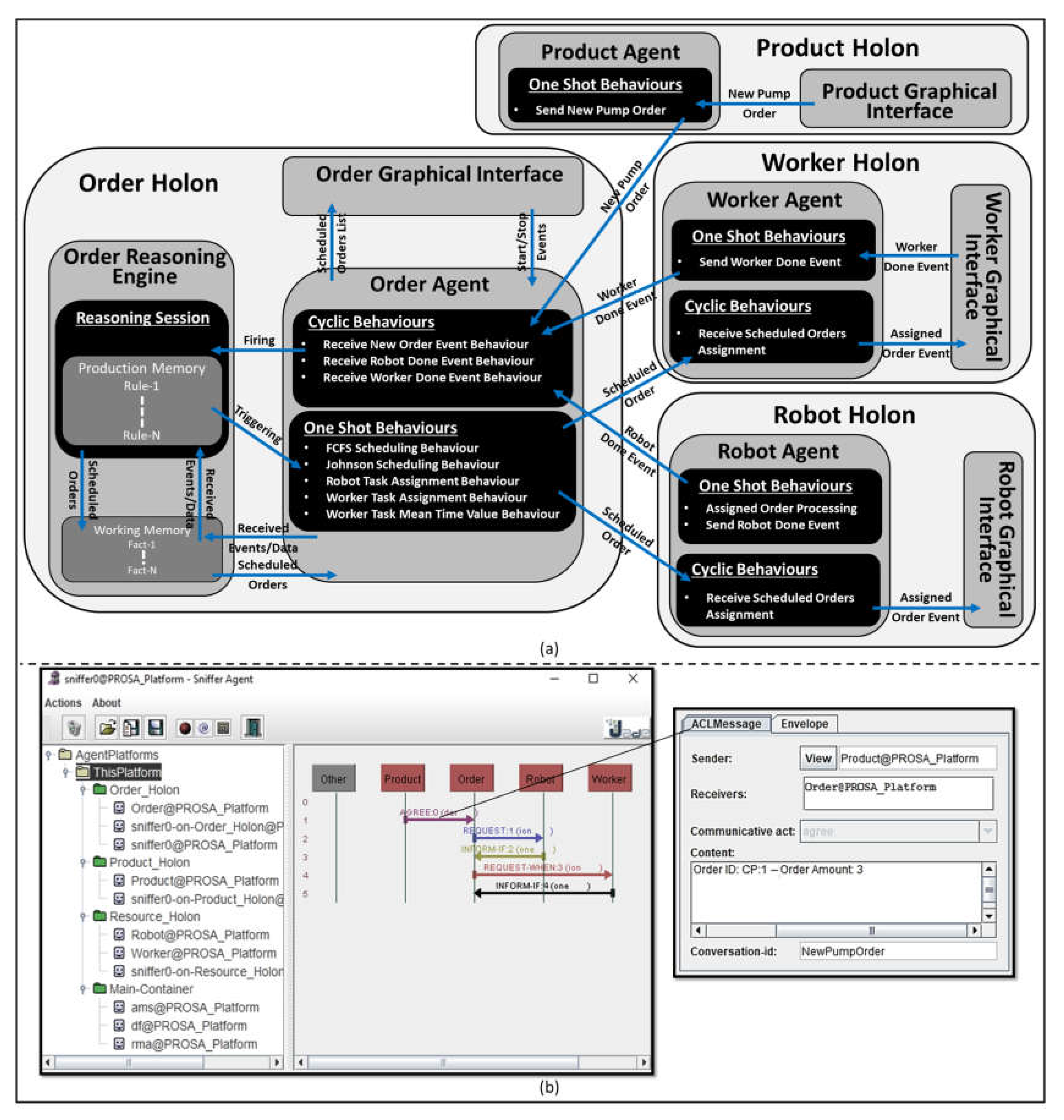
Figure 8.
Case-study scheduling results.

Figure 9.
Gantt chart of the case-study scheduling.


Table 1.
Johnson Scheduling vs. First Come First Serve Scheduling.
| Unscheduled Jobs List | First Come First Serve Scheduling | Johnson Scheduling | ||||||
|---|---|---|---|---|---|---|---|---|
| Ji | TPi@M-A | TPi@M-B | Ji | TOi@M-A | TOi@M-B | Ji | TOi@M-A | TOi@M-B |
| J1 | 10 | 5 | J1 | 0:10 | 10:15 | J2 | 0:6 | 6:18 |
| J2 | 6 | 12 | J2 | 10:16 | 16:28 | J4 | 6:14 | 18:28 |
| J3 | 8 | 9 | J3 | 16:24 | 28:37 | J3 | 14:22 | 28:37 |
| J4 | 8 | 10 | J4 | 24:32 | 37:47 | J5 | 22:34 | 37:44 |
| J5 | 12 | 7 | J5 | 32:44 | 47:54 | J1 | 34:44 | 44:49 |
Table 2.
Johnson Scheduling Based On RTC (Robot Time Constant) and WMTV (Worker Mean Time Value).
| Unscheduled Jobs List | Johnson Scheduling Case-1: RTC ≤ WMTV | Johnson Scheduling Case-2: RTC ≥ WMTV | ||||||
|---|---|---|---|---|---|---|---|---|
| Ji = (Oi, ni) | RTPi | WTPi | Ji | RTPi | WTPi | Ji | RTPi | WTPi |
| J1 = (O1, n1) | RTC * n1 | WMTV * n1 | J1 | RTC * n1 | WMTV * n1 | J2 | RTC * n2 | WMTV * n2 |
| J2 = (O2, n2) | RTC * n2 | WMTV * n2 | J2 | RTC * n2 | WMTV * n2 | J1 | RTC * n1 | WMTV * n1 |
≤ ≡ Less than or equal to, ≥ ≡ Greater than or equal to, * ≡ Multiplied by.
Table 3.
Drools Scheduling and Order Assignment Decision Table.
| Event | State Rule | Action | State Explanation | ||||||
|---|---|---|---|---|---|---|---|---|---|
| Start Flag | Stop Flag | Worker Done Counter | Robot Status | Worker Status | Received Orders List | Scheduled Orders List | |||
| New Order Event | True | False | Equal to 0 | Free | Don’t Care | Don’t Care | Don’t Care | -FCFS scheduling -Robot order assignment | -New order event is received at the very beginning. -New order event is received after the robot is done with all the previously assigned orders, while the worker has not finished the first assigned order. |
| New Order Event | True | False | Equal to 0 | Busy | Don’t Care | Don’t Care | Don’t Care | -FCFS scheduling | -New order event is received while the robot is executing one previously assigned order, while the worker has not finished the first assigned order. |
| New Order Event | True | False | Greater than 0 | Free | Don’t Care | Don’t Care | Don’t Care | -Johnson scheduling -Robot order assignment | -New order event is received after the robot is done with all the previously assigned order, while the worker has finished at least the first assigned order. |
| New Order Event | True | False | Greater than 0 | Busy | Don’t Care | Don’t Care | Don’t Care | -Johnson scheduling | -New order event is received while the robot is executing one previously assigned order, while the worker has finished at least the first assigned order. |
| Robot Done Event | True | False | Equal to 0 | Don’t Care | Free | Not Empty | Don’t Care | -FCFS scheduling -Worker order assignment | -The robot finished one assigned order while the worker is free and has not assigned any previous order. |
| Robot Done Event | True | False | Equal to 0 | Don’t Care | Busy | Not Empty | Don’t Care | -FCFS scheduling | -The robot finished one assigned order while the worker is executing the first assigned order. |
| Robot Done Event | True | False | Greater than 0 | Don’t Care | Free | Not Empty | Don’t Care | -Johnson scheduling -Worker order assignment | -The robot finished one assigned order while the worker is free and has finished at least one assigned order. |
| Robot Done Event | True | False | Greater than 0 | Don’t Care | Busy | Not Empty | Don’t Care | -Johnson scheduling | -The robot finished one assigned order while the worker is busy and has finished at least one assigned order. |
| Worker Done Event | True | False | Don’t Care | Don’t Care | Don’t Care | Don’t Care | Not Empty | -Calculate the order execution average time -Worker task assignment | -The worker finished one assigned order while still there is at least one order in the scheduled orders list. |
| Worker Done Event | True | False | Don’t Care | Don’t Care | Don’t Care | Don’t Care | Empty | -Calculate the order execution average time | -The worker finished one assigned order while the scheduled orders list is empty. |
© 2017 by the authors. Licensee MDPI, Basel, Switzerland. This article is an open access article distributed under the terms and conditions of the Creative Commons Attribution (CC BY) license (http://creativecommons.org/licenses/by/4.0/).
Share and Cite
MDPI and ACS Style
Sadik, A.R.; Urban, B. Flow Shop Scheduling Problem and Solution in Cooperative Robotics—Case-Study: One Cobot in Cooperation with One Worker. Future Internet 2017, 9, 48. https://doi.org/10.3390/fi9030048
AMA Style
Sadik AR, Urban B. Flow Shop Scheduling Problem and Solution in Cooperative Robotics—Case-Study: One Cobot in Cooperation with One Worker. Future Internet. 2017; 9(3):48. https://doi.org/10.3390/fi9030048
Chicago/Turabian StyleSadik, Ahmed R., and Bodo Urban. 2017. "Flow Shop Scheduling Problem and Solution in Cooperative Robotics—Case-Study: One Cobot in Cooperation with One Worker" Future Internet 9, no. 3: 48. https://doi.org/10.3390/fi9030048
Note that from the first issue of 2016, this journal uses article numbers instead of page numbers. See further details here.