Energy-Aware Adaptive Weighted Grid Clustering Algorithm for Renewable Wireless Sensor Networks


1
School of Electronic and Information Engineering, Hebei University of Technology, Tianjin 300401, China
2
Department of Computer Science and Engineering, University of Engineering and Technology (UET), Lahore 54890, Pakistan
3
Department of Electrical, Electronic and Information Engineering (DEI), University of Bologna, 40136 Bologna, Italy
*
Author to whom correspondence should be addressed.
Future Internet 2017, 9(4), 54; https://doi.org/10.3390/fi9040054
Submission received: 23 July 2017
/
Revised: 16 September 2017
/
Accepted: 19 September 2017
/
Published: 23 September 2017
Abstract
:Wireless sensor networks (WSNs), built from many battery-operated sensor nodes are distributed in the environment for monitoring and data acquisition. Subsequent to the deployment of sensor nodes, the most challenging and daunting task is to enhance the energy resources for the lifetime performance of the entire WSN. In this study, we have attempted an approach based on the shortest path algorithm and grid clustering to save and renew power in a way that minimizes energy consumption and prolongs the overall network lifetime of WSNs. Initially, a wireless portable charging device (WPCD) is assumed which periodically travels on our proposed routing path among the nodes of the WSN to decrease their charge cycle time and recharge them with the help of wireless power transfer (WPT). Further, a scheduling scheme is proposed which creates clusters of WSNs. These clusters elect a cluster head among them based on the residual energy, buffer size, and distance of the head from each node of the cluster. The cluster head performs all data routing duties for all its member nodes to conserve the energy supposed to be consumed by member nodes. Furthermore, we compare our technique with the available literature by simulation, and the results showed a significant increase in the vacation time of the nodes of WSNs.
1. Introduction
Wireless sensor networks (WSNs) consist of spatially distributed autonomous devices using sensors to monitor physical or environmental conditions. A WSN system incorporates a gateway that provides wireless connectivity back to the wired/wireless world and distributed nodes equipped with radio transceivers, microcontrollers, external memory, and electronic circuits for interfacing with the sensors, and small-embedded batteries. WSNs also find their applications in military surveillance [1,2], geo-fencing [3], healthcare monitoring [4,5], environmental monitoring [6,7,8], and remote monitoring [9]. Additionally, sensors are the primary key sources of Big Data Analytics—the process of examining large data sets for customer-focused business decisions and market trends [10,11]. The main limitation of WSNs is their batteries. Due to the finite capacity of batteries, the lifetime performance of WSNs is a fundamental bottleneck. The nodes consume energy for sensing, communicating, and data processing. The energy used in data communication is higher than any other process [12,13].
It is well established that power maximization approaches such as conservation of energy [14,15], ambient power or environmental energy harvesting [16,17,18,19], incremental deployment and battery replacement [20,21] exert a profound influence on the enhancement and enrichment of the lifetime of WSNs. In addition, these techniques evaluate the lifetime increment of the batteries, but on the contrary they are unable to reduce energy consumption. Harvesting natural energy, such as solar power [16,18], vibrations [17], and the wind [19] is solely dependent on climatic conditions [22]. Thus, the source of energy is random and potentially sporadic, such as for solar-powered nodes which are exclusively dependent on the influx of the sun rays.
The commercialization [23] of wireless charging (power transfer) technology is a promising option to address the energy limitations in WSNs [24]. Kurs et al. [25,26] introduced the concept of wireless power transfer (WPT), which transfers power through magnetic fields between two coupled coils, a phenomenon called coupled resonators, as a function of the geometry, distance, and electrical properties of the devices used. The wireless power transfer proposed by this research group has high efficiency and the potential to charge devices from a relatively long distance. The wireless power transfer method developed by Kurs et al. has numerous advantages such as the WPT transmits energy via a non-radiative recombination process. The power transmission range can be further improved by the installation of repeaters between power transmitting and receiving devices.
In contrast to battery substitution and wireless power transfer techniques, the innovation of the renewable wireless charging approach permits a charger to transfer power to the nodes remotely without strict management and environmental effects (air, dirt and chemicals) between them [27]. In the last decade, several researchers have conducted research pertaining to wireless charging frameworks, but herein, we have attempted to develop a technique which caters to the needs of WSNs i.e., a rechargeable wireless network which remains operational and minimizes energy consumption. Our research pathways have been delineated as below:
1. In the environment of single-hop data routing, the distance between the nodes and base station may vary due to their randomly dispersed deployment which causes high-energy consumption. To overcome this, a weighted clustering algorithm is proposed which divides all nodes, based on their positions and remaining energy levels, into multiple groups called clusters. A cluster head is appointed to each cluster so that nodes can conserve energy via direct communication with their cluster head. Each cluster head has a higher amount of energy which is responsible for communicating with the base station and other nodes as well. It reduces the consumption of energy compared with the single-hop routing and Geometric Routing Protocol (GR-Protocol).
Shuo et al. suggested a feasible traveling path for the wireless charging vehicle (WCV) to reduce the computation time [28]. Upon following that feasible path, the WCV decreases the computation time with the help of a geometric heuristic technique. GR-Protocol divides the whole network into small grids. The sizes of all grids remain the same or lower than the maximum defined range. The GR-Protocol notifies the center location at which the WCV is staying to recharge all member nodes via a one-to-many wireless power transfer approach. Thus, the GR-Protocol minimizes the computation time to elongate the lifetime of the WSN.
2. A novel traveling path, based on the shortest path algorithm, for the wireless portable charging device (WPCD) is devised to cover all the nodes during the charging process. This optimized path increases the vacation time that is responsible for the overall network lifetime. The aforementioned proposed techniques are associated with each other to minimize the transmission energy and maximize the vacation time of the WPCD. The simulation results show that the proposed method outperforms the existing methods regarding vacation time, remaining energy, energy consumption and arrival time of the WPCD at every node.
The remaining paper is structured as follows: Section 2 describes the related work. The preliminary description of the problem and system model is mentioned in Section 3. In Section 4, we have proposed the traveling path of the WPCD followed by the weighted grid-clustering algorithm, which is written in Section 5. The simulation and performance assessment are presented in Section 6. Section 7 concludes the paper with discussion of a future research direction.
2. Related Work
Energy efficiency is a critical issue for a WSN. To make a WSN effective in hazardous environments is a big challenge. To date, the bulk of research concerning the lifetime performance of WSN has been done. Rahimi et al. explored the mobility concept of nodes in search of energy [29]. Mobile nodes can transfer power to the immobile nodes to elongate the lifetime of the WSN.
Kurs et al. upgraded an innovation for charging numerous devices concurrently by using appropriate coupled magnetic resonators [26]. Yi Shi et al. considered the issue of scalability for nodes in rechargeable wireless networks [30]. Shi et al. described the optimization of multi-hop dynamic data routing and scheduling for the wireless charging vehicle by using the wireless power transfer technique [31]. Motivated by their research in wireless power transfer, we have explored both single-hop routing and multi-hop routing in this study by using the proposed weighted grid clustering algorithm. Additionally, the WPCD travels periodically along the proposed route and charges the nodes that come along its way. The total distance from the first node to the last node, that the WPCD navigates in the network is called the traveling cycle, whereas the entire time which the WPCD spends at a rest station (RS) to recharge its battery for the next cycle is called vacation time.
Fu et al. introduced the concept of energy synchronization charging (ESync) between nodes based on a set of nested traveling salesman problem (TSP) tours to enhance the charging travel distance as well as the charging delay of sensor nodes [32]. Li et al. developed an approach, which used wireless power transfer for electrical vehicles in their work [33]. Chen et al. proposed an energy efficient GR-Protocol to minimize energy consumption and time complexity through the calculation of traveling (computation) time for WCV [28]. Of late, they have also developed a framework for simulating a WSN environment for wireless power transfer using mobile vehicles [34].
Most of the existing work on rechargeable wireless sensor networks investigates the optimized path for the WPCD using an approach that increases the vacation time. Previous researchers consider mathematical optimization to optimize an objective function based on the traveling path of the WPCD and energy model. However, these optimization algorithms are not economically feasible for the sensor nodes and need experts to implement them. Assuming all these considerations, we proposed a unique traveling path for the WPCD based on the shortest path to increase its vacation time, which is relatively economical to compute.
3. The Preliminary Description of the Problem
3.1. Problem Formulation
To formulate this energy issue, N number of nodes equipped with the power-receiving batteries distributed throughout the two-dimensional area, a rest station (RS), a base station (BS), and a WPCD are considered. The deployed nodes are considered as static (fixed) nodes. Notations for the entire network model are defined in Table 1.
The WPCD starts its journey from a RS and travels among all the nodes to transfer power via WPT. After completing the cycle, it recharges its own battery at the RS. In a practical environment, the WPCD can be the vehicle driven by a person on the proposed traveling path. If a person is driving the vehicle, he can also save the WPCD from the hurdles found during its traveling path. The WiTricity Corporation has numerous light weighted, low power and small products that can be installed on the WPCD for wireless power transfer [35]. For instance, the WPCD can be equipped with the WiTricity-3300 which weighs 3.6 kg and is 20 cm × 28 cm × 7 cm in size. In our scenario, energy and maintenance cost required for the moving of the WPCD is not considered as it is not a bottleneck.
A set of N nodes deployed in a two-dimensional region is displayed in Figure 1.
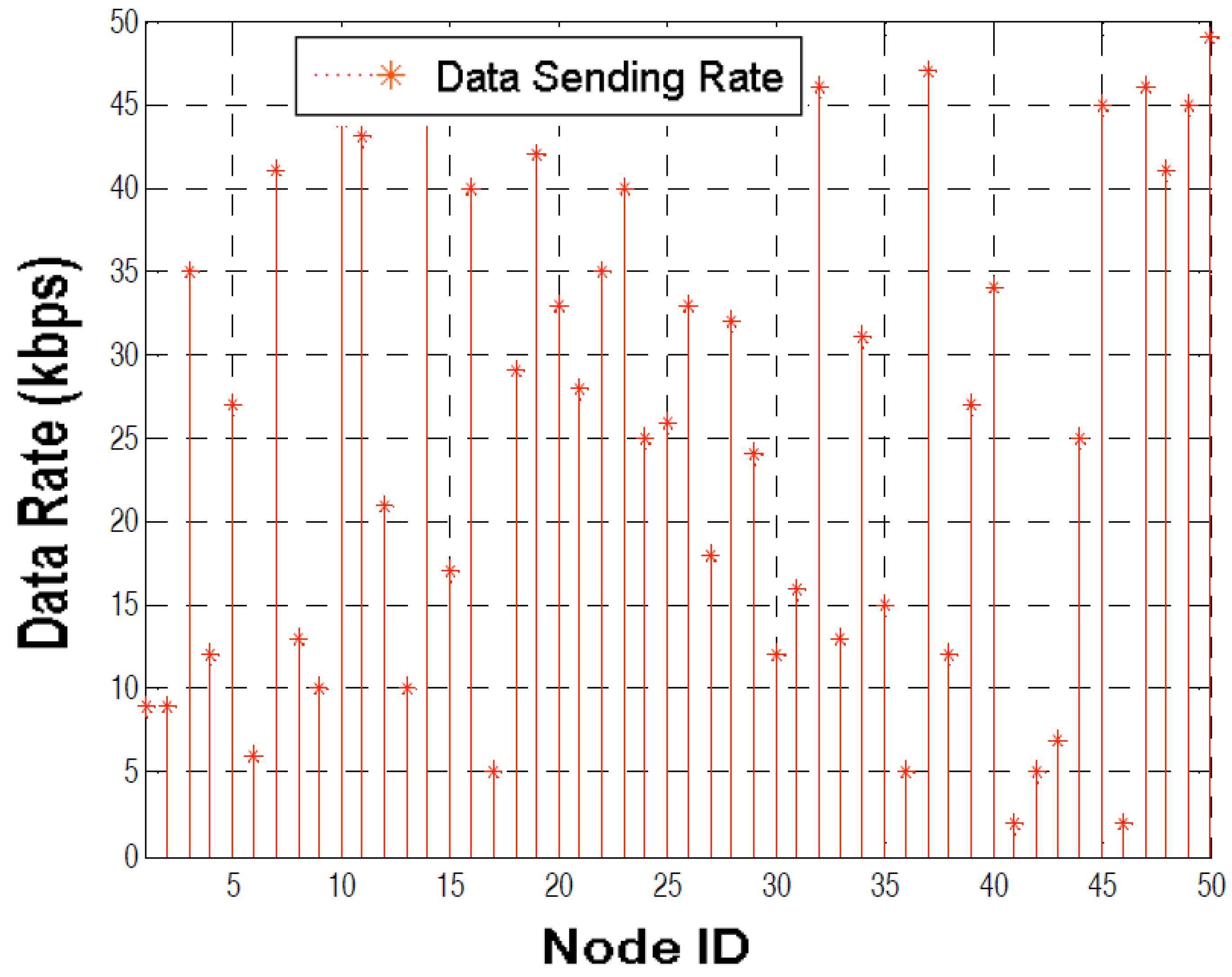
All the nodes in the wireless sensor network are assumed to be facilitated with a battery of maximum energy Emax. The energy of the node decreases with the passage of time and then dies out if the energy reaches below the Emin. Thus, Emin is the minimum energy required to keep a sensor node functional. Each node senses data and forwards it to the base station. The flow rate is different with time because our energy consumption model is handling the rate of flow of data and routing as well. Further, each node sends data at the rate of Ri (bps), where i is any single node in network N.
Shi et al. described the renewable energy cycle of the WPCD [31]. In the proposed energy cycle, the WPCD starts its journey from a RS and remains engaged for recharging the battery of all sensor nodes that come along its way. We assume that the WPCD has adequate energy stored to charge all the sensor nodes in the network. The WPCD will traverse all the nodes for recharging the power with the velocity of V (m/s). After leaving from the RS, the WPCD starts to charge the first node i. As mentioned above, the traveling path of the WPCD, is decided by the shortest path algorithm. The rate at which power is transferred via WPT, from the WPCD to the node’s battery is denoted as U. The WPCD spends τi time to recharge the first node i and then moves to the nearest node j. The communication radius of the WPCD is denoted as Rc. Using Rc, the WPCD calculates the distance of the node from its location and selects the closest node for charging. Once the first node is charged, WPCD recalculates the distance for the next closest node and this cycle will continue until the completion of recharging all the nodes. After completing the full round of the network, the WPCD returned to the rest station to recharge its battery.
3.2. System Model
To handle the data flow rate and energy consumption for each node of the renewable wireless sensor network, the following energy model has been used. This model represents a routing scheme with the following flow balance constraints:
Here gij and giB(t) are the data flow rate from sensor node i to j and base station. And, gki(t) is the rate of gathering data in a time t. Equation (1) implies the rate of generating data at node i plus the rate of receiving data from any other node k is equal to the rate of sending data from node i to j and the base station. Here, the energy consumption of a node during a renewable cycle must meet two significant requirements:
- The energy of each node remains equal both at the beginning and at the end of one renewable cycle during the time of τ.
- To make a node operational, the energy of the node is never less than the Emin.
We handle the above issues by the following energy consumption constraints:
There is some energy consumption for data sending and data gathering. Equation (2) is responsible for energy consumption in the network, as pi(t) is the rate of energy consumption for node i over a time t, whereas ρ is denoted as the energy consumption coefficient for receiving data measured by the rate of generating data (Ri). Accordingly, in this energy model, represents the energy consumption rate for gathering data. , is the rate of energy consumption for sending data from the sensor nodes.
As Emin is a threshold value, the proposed model assumes that the energy of each node is not less than this threshold value. A charge cycle is divided into three main parts:
- The WPCD starts its journey from a RS and arrives at node i on the prescribed path using the shortest path algorithm.
- During time τi, the WPCD charges the battery of node i remotely via wireless power transfer technology.
- Then, the WPCD revolves towards the next node to supply power. Finally, it takes a vacation at the RS until the start of the next cycle. Vacation time denoted as τvac, helps the WPCD to energize its battery for the next charge cycle whereas τ is the complete time required for one charge cycle.
To cope with the performance limitations on a network; the layout is transferring the power to each node intermittently so that its energy never falls below Emin. To increase τvac for the WPCD at the RS, we need to maximize the objective function (i.e., ) as presented in [36]. As per this objective function, we can either maximize the value of the numerator (i.e., τvac) as a vacation time or minimize the value of the denominator (i.e., τ) as overall traveling time.
4. Proposed Travelling Path for the WPCD
Kumar et al. presented an energy efficient algorithm, which minimizes the consumption of energy based on the value of bit error probability [37]. By using the shortest path algorithm, we proposed a route for the WPCD to travel inside the network.
First, a message broadcasts through the WPCD to get the location information about all nodes. Second, the WPCD figures out the shortest distance between the nodes based on the location information received. Third, it selects the nearest node first to recharge its battery. Fourth, it moves to the next closest node to recharge its battery and this cycle goes on until each node gets fully recharged. Finally, the WPCD returns to the RS, where it gets itself recharged before initiating the next recharge cycle.
To understand this algorithm, we assume three nodes with their prescribed location on U(y1, z1), V(y2, z2), and W(y3, z3). The WPCD starts to find the distance of all nodes from its origin (0, 0). The distances of the nodes U, V, and W are denoted by d1, d2, and d3 respectively.
The WPCD calculates the distances d1, d2, and d3 using the above formulas and if it finds d1 to be the shortest distance for node U from its origin, it moves towards node U for recharging its battery to its fullest. Once the WPCD recharges the battery of node U, then it removes d1 from its routing table. The same comparison goes for nodes V and W, if it finds d3 smaller than d2, the WPCD will travel to the W node and recharge it to its fullest. After recharging the battery of node W, d3 will also be removed from the routing table. Later, the distance d3 of the node V will also be removed from the routing table after charging its battery by the WPCD. The cycle goes on until all, in this case, d1, d2 and d3 get removed from the routing table using the following comparison formulas.
With the help of following general equations, comparative calculation of the remaining distance continues among the nodes until every node gets reached for recharging.
The symbols of y and z are the coordinates of the nodes, where i, j and k are member nodes from the total number of nodes N which can be expressed by the following set:
Total number of the nodes in the entire network model = {i, j, k.......N}.
5. Weighted Grid Clustering Algorithm
5.1. Weighted Grid Clustering
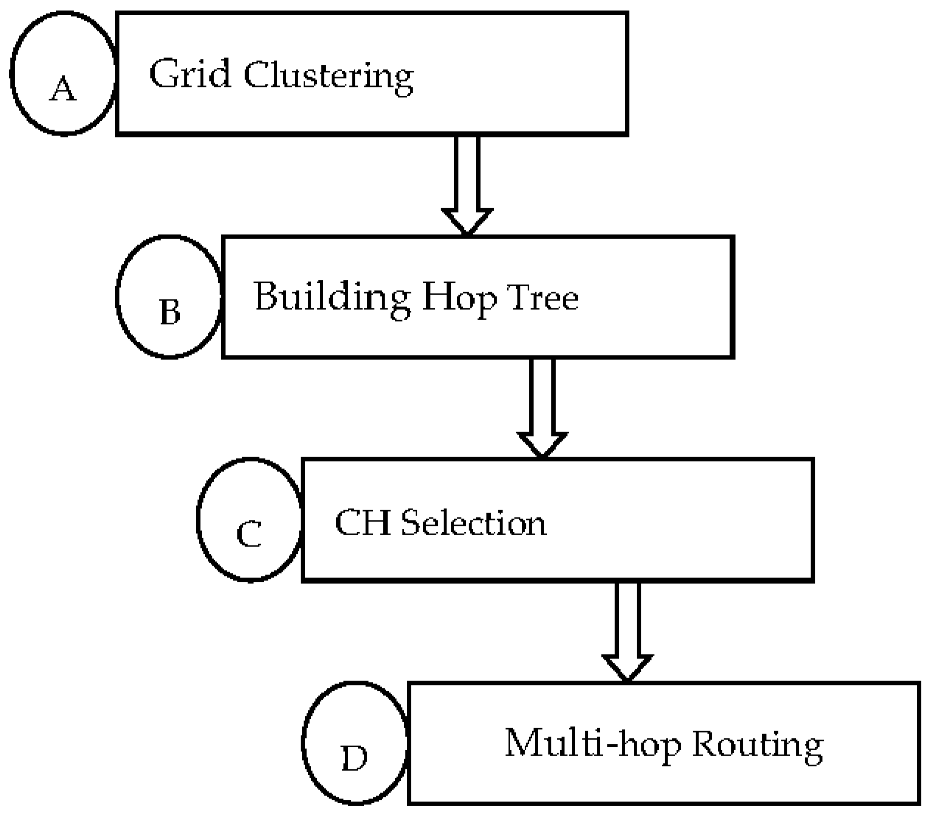
For energy conservation, we propose a technique which consists of four models namely grid clustering, building the Hop tree, selection of a dynamic cluster head, and multi-hop routing and Hop tree update [38].
The process starts with the division of even-sized grids in the WSN. Once the grid structure is built, a node called sink broadcasts the Hop configuration message. This message helps in selecting a dynamic cluster head (CH) among all the other member nodes by their remaining battery capacity. Subsequently, the corresponding cluster head in the grid collects the data from all its member nodes and forwards it to the base station. The overall routing process is shown in Figure 2.
The grid-based clustering technique directly depends on the formation of a CH, which plays the role of a gateway between nodes and the base station. The sensor nodes send their data to the CH and then the CH manages all the functions of delivering data. Moreover, the CH acts as a bridge between the nodes for information exchange. The CH can send the data to the concerned node and base station instantaneously, or it uses any other CH as a medium if needed. In conclusion, two main observations for saving more energy are noticed, as follows:
- A CH saves energy and space by creating only one routing table for all nodes rather than making an individual routing table for each node as in single-hop routing.
- A CH schedules the activities for all nodes in its specified region. These activities are maintained by broadcasting a message to all the member nodes. This message contains different schedules in which nodes can perform their operations (sending/receiving) with the CH and other nodes as well. After that, nodes can turn on their sleep mode.
After completing the clustering structure, all the nodes are free to transmit data locally with the help of the CH. Then, the CH forwards data to the base station via neighbor grids. The proposed scenario describes that grid-based routing provides the multi-hop routing between CHs and it also prevents the long range data transmission.
5.2. Construction of the Hop Tree
The area of the grid is assumed to be a square with length of size, s. A division of the square-based grid helps easy coordination among the nodes. Each node in a specific grid calculates its grid coordinates (X, Y) according to the node’s location (x, y) with the help of the following equation:
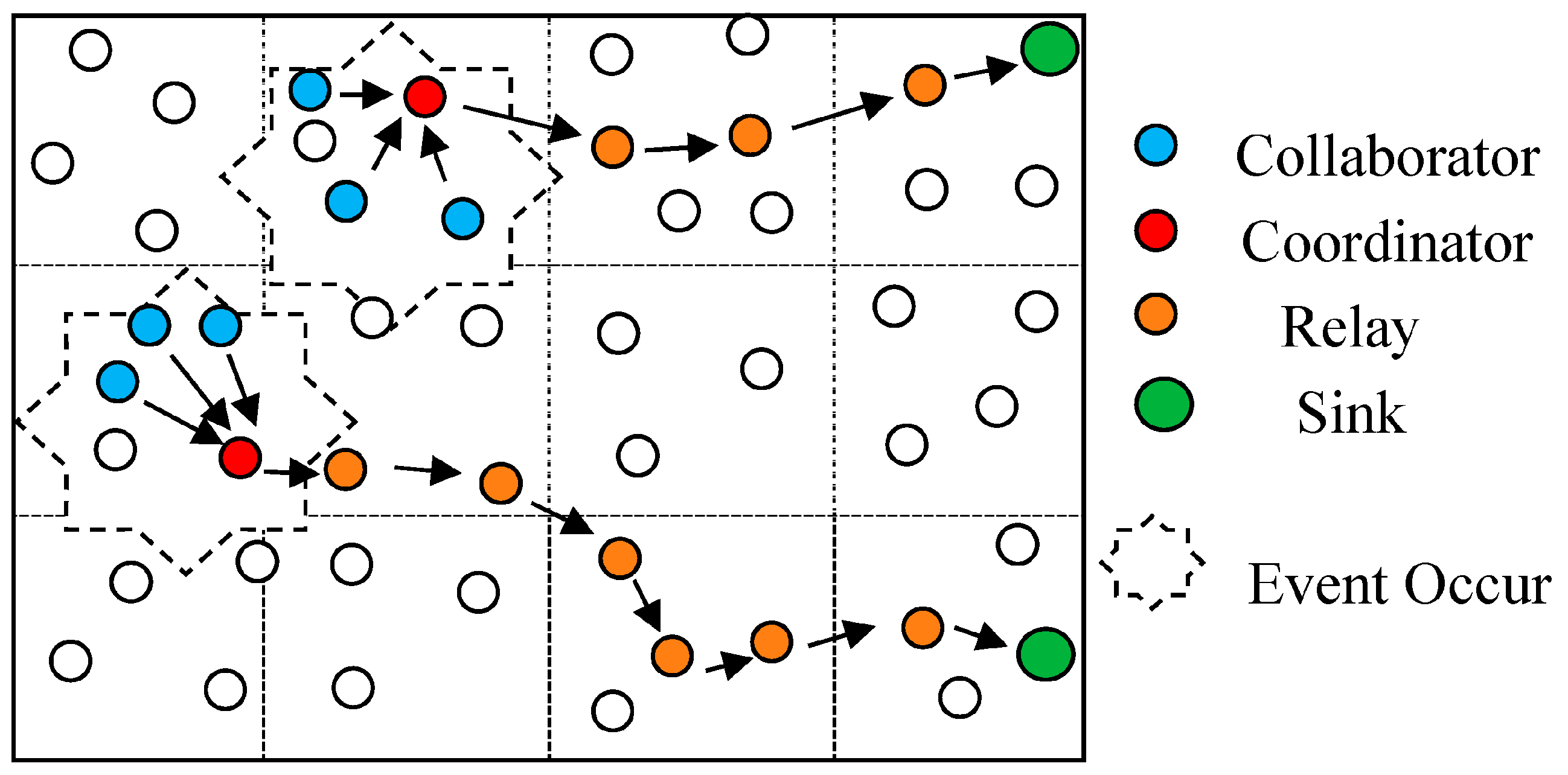
The location of the node (x, y) is found using a GPS. Four technical roles for different nodes have been assigned during the whole procedure of cluster routing [39]. These are as follows:
- Sink: A node which is responsible for accumulating data from the following defined coordinator and collaborator nodes.
- Relay: These nodes receive data from the coordinator and forward it to the sink.
- Collaborator: If there is some data from any node, then these nodes are responsible for sending this data towards the coordinator.
- Coordinator: This node accumulates all the data from the collaborator and sends the result towards the sink. These roles of the sensor nodes are shown in Figure 3.
The pseudo code of this process is given in Algorithm 1.
| Algorithm 1. Building of the Hop Tree |
|
Construction of the Hop tree phase calculates the distance between the nodes and the sink. This distance is calculated by the number of hops between them. The sink node initiates this stage with a Hop Configuration Message (HCM) to all the member nodes of the entire renewable sensor network. This HCM is comprised of two fields, namely the Node Identifier (NID) and HopToTree (HTT). NID carries the identification of the next node, whereas HTT stores the distance from nodes to sink in several hops. At the start of the tree construction, the HTT value for the sink node is stored as 1 whereas the HTT values for remaining nodes are stored as infinity. After receiving the HCM message, each node compares if the value of HTT in the HCM message is less than the value of the HTT which is already stored as 1. At the same time, if the first sending of any member node u is also true then the condition of our algorithm proves true. Then each member node updates the storedvalue of the NextHop variable with the value of the HCM (HTT and NID). On the contrary, the value of the HCM message will also be updated regarding the NextHop variable, HTT and NID as described on line 6–9 of Algorithm 1. Inversely, if the condition is false, the node deletes the received HCM and HTT. The stored values of HCM and HTT remain the same. This procedure repeatedly occurs to configure the complete network.
5.3. Selection of Cluster Heads
After the construction of the Hop Tree, the next stage is the selection of cluster heads, which is described in Algorithm 2.
| Algorithm 2. Selection of a Cluster Head among Clusters |
|
The higher energy nodes in the network are the best candidates for CH selection. The algorithm starts selecting the CH when an event occurs, i.e., two nodes want to communicate with each other or with the base station. This phase depends on the weights of the nodes. Each node calculates its weight with its remaining energy (residual energy), the distance between the node to the sink and its buffer size.
The node distance may vary from the sink, so the node which is closest to the sink node will be more eligible. If there is a tie between two nodes having the same distance, then the node with the smallest NID wins the race. The other option is energy calculation among all the sensor nodes, these nodes, which frequently participate in the communication, are exhausted rapidly due to more usage of their energy than other nodes that contain less data and hence use a lesser amount of energy. For effective CH selection, each node must know its remaining energy, since election takes place based on the highest remaining energy among the sensor nodes. After that, the buffer size of that node will be calculated to accumulate the weight (Wu). Finally, a single node with maximum weight is selected as a cluster head, which is then broadcast to the entire network member nodes. Every member node of the grid remembers its CH and all the event detection reports are sent directly to the CH.
During the CH selection, we assume S number of nodes within one cluster, where u is a single node in S.
where Eru denotes the residual energy of that node u, Du denotes the distance between the member node u and the sink node. The remaining buffer size of the node u is designated by the Bu; and α, β, γ are weights. These weights (α, β, γ) are assigned to Eru, Du and Bu respectively as expressed in the Equation (12). The following criteria for assigning the weights are considered:
Wu = Eru × γ + Du × β + Bu × α
γ > β > α and α + β + γ = 1
The value of γ cannot be greater than 0.45 as the maximum energy (Emax) of each node is 10,800 J.
The sum of these weights is calculated with 1 as a probability factor for most appropriate selection of the CH.
This criterion is defined after the empirical evaluation of each node’s status. During the calculation process of Wu, the most important factor is residual energy which is directly dependent on the initial Emax of a particular node. Thus, the highest value of weight γ is assigned to the residual energy which is measured in Joule. The value β is assigned as the second significant weight to the buffer size of the node which can be calculated in KB. Lastly, the smallest value of weight α is assigned to the distance. The distance Du is measured regarding the number of hops (e.g., node u has seven hops to the sink node). We have calculated the most suitable constant values of α = 0.2, β = 0.35 and γ = 0.45 after the analysis of different nodes during different simulations which is depicted in Figure 4.
With the help of the Equations (12) and (13), a weighted sum of the nodes is calculated, and the cluster head is selected. Now, each CH is responsible for collecting information from the member nodes and forwarding aggregated data towards the sink node.
5.4. Multi-Hop Routing
The cluster head is now responsible for route formation and routing the data towards the sink node. The routing of data is divided into two main types:
- Inter cluster data routing
- Intra cluster data routing
For route selection and data transfer, the node, which is considered as a coordinator, forwards the route selection ACK message to the NextHop. After receiving the message, NextHop replies to the coordinator and thus the hop tree updating process starts. These steps go on repeating until the sink node is found or a node is reached which is already located on the route. Once a route is established, multi-hop data routing also starts. The main goal of this phase is to update the HopToTree value of all the nodes so that each node obtains the new next-hop ID for further routing. Finally, the new relay node initiates the hop tree updates after implementing the Hop Tree Algorithm.
When a member node of a CH has some data to send, CH will wait for the data from any other member node. CH will collect the data from its entire descendants and forwards the aggregated data to the NextHop node. Using this routing technique, energy consumption is highly reduced. The whole process is explained in Algorithm 3.
| Algorithm 3. Multi-hop routing and Hop Tree update |
|
6. Simulation and Performance Assessment
6.1. Simulation Environment
Simulation results of the proposed solution are illustrated in this section by both tabular and graphical representations. We evaluated our proposed method with the single-hop routing and GR-Protocol algorithm regarding vacation time, remaining energy and energy consumption for each node. The default parameters used in the simulation are written below in Table 2.
The computation and simulation were carried out in MATLAB [40]. The hardware requirements include an Intel Core i5 and minimum 4 GB of RAM. In all instances, the time of the WSN was measured in seconds. Sensor nodes are deployed in a 1000 × 1000-m square area by using omni-directional antenna parameters.
For each node, we picked a regular NiMH battery equipped with a charge receiving coil. The maximum and minimum energy for each node are considered on the specifications of NiMH batteries where the nominal cell voltage is 1.2 V and the electricity quantity is 2.5 Ah [41]. Accordingly, we have the values of Emax and Emin as follows:
- Emax = 1.2 × 2.5 × 3600 seconds = 10,800 J = 10.8 kj
- Emin = 0.05 × Emax = 540 J = 0.54 kj
Simulation is initialized with the maximum amount of energy charge at each node. If the energy level of any node reaches below the Emin (540 J), the node does not remain operational. The simulation model is like the numerical analysis that uses different numerical approximations. First, the proposed shortest traveling path for the WPCD is implemented for the maximization of the objective function (i.e., ). The parameters (i.e., τvac, τ) are calculated from numerical computations. Subsequently, as in the module on model design, the provable-optimal solution is developed for routing protocol based on the proposed weighted grid clustering, arrival time of the WPCD, charging time of the single node and total charge cycle time of the entire network. An energy consumption model is handling the energy consumed by the WSN in single-hop and dynamic (grid clustering) routing. Comparing numerical results shows the overall behavior of the network linked with the renewable charge cycle. Finally, to show the uniformity of the results, mean and variance are calculated by repeating the experiment in different situations which are as follows:
- Different types of routing scenario (single-hop and grid clustering)
- Diverse values of weighted parameters (α, β and γ are shown in Figure 4)
- Different locations of deployed nodes (11 different cases to compute the mean and variance)
- Considering the special situations of nodes (busy nodes, CH nodes and idle nodes)
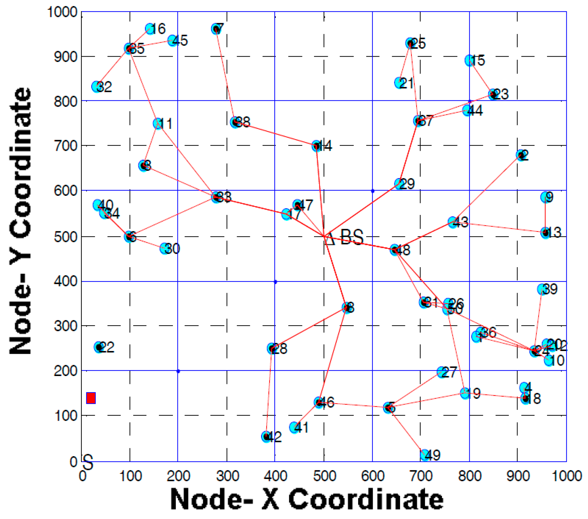
Generally, the WPCD traverses the randomly deployed node on the physical path, P. Deployment of nodes is shown in Figure 5, Figure 6 and Figure 7 during different simulation environments. In Figure 5, the red dot is the WPCD, moving in the WSN to charge the battery of each node, whereas the triangle symbol is the BS. Figure 6 presents the clustering scope as red lines in one simulation case. Figure 7 displays the square-sized grid division in another case. Figure 7 also shows the CH as a black colored node in the designated grid. After completing the deployment, simulation ran for one hour to get the desired results. Observing the graphical results, it was concluded that the energy consumption in grid clustering routing is less for data transmission as compared with typical single-hop routing and GR-Protocol.
6.2. Results
The simulation results of the first 20 nodes at the same coordinate location are presented in Table 3. The first column of the table shows the particular node approached by the WPCD. Node locations for single-hop routing and multi-hop routing are mentioned in the second and the fifth column respectively. Simulation results are evaluated with the help of column 3, 4, 6, and 7. When the WPCD approaches any node, the remaining energy (minimal energy) of that node increases due to the implementation of proposed grid clustering routing, which is demonstrated in column 5. The significant increase in minimal energy of the nodes can be compared in column 4 and column 7.
Additionally, the data sending rate in the renewable WSN can be viewed in Figure 8.
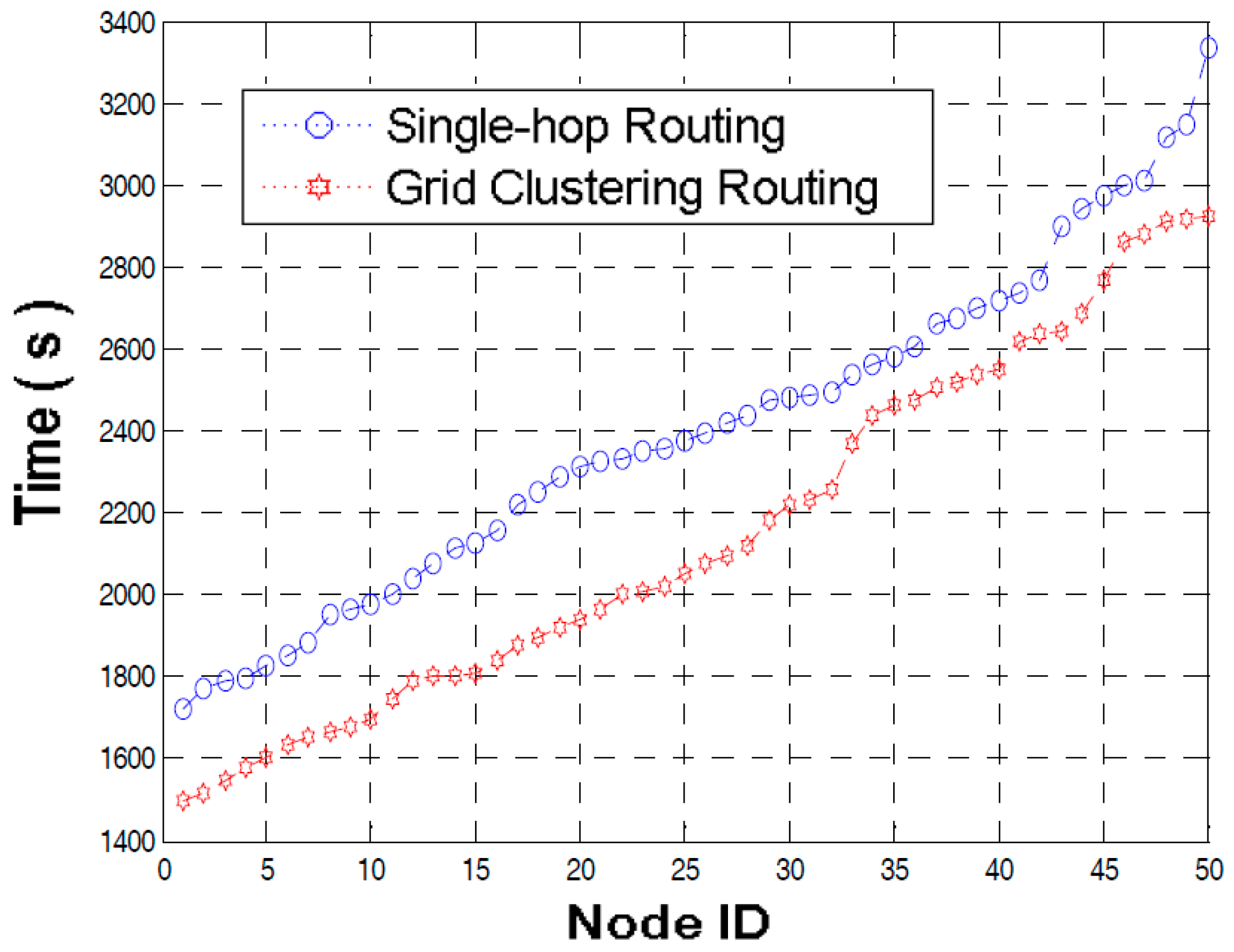
Single-hop routing requires a long time to initiate the node’s battery recharge via WPT as compared with the weighted grid clustering routing. The proposed solution gives shortened arrival time (the time to initiate the node’s battery recharge) for the WPCD at each node in the recharge cycle. The metric for the arrival time of the WPCD is ai(t) as shown in Figure 9, which needs to be decreased. So, the graph represents the single-hop routing with a blue circle line which has higher arrival times than the proposed weighted grid clustering routing, shown as a red star line.
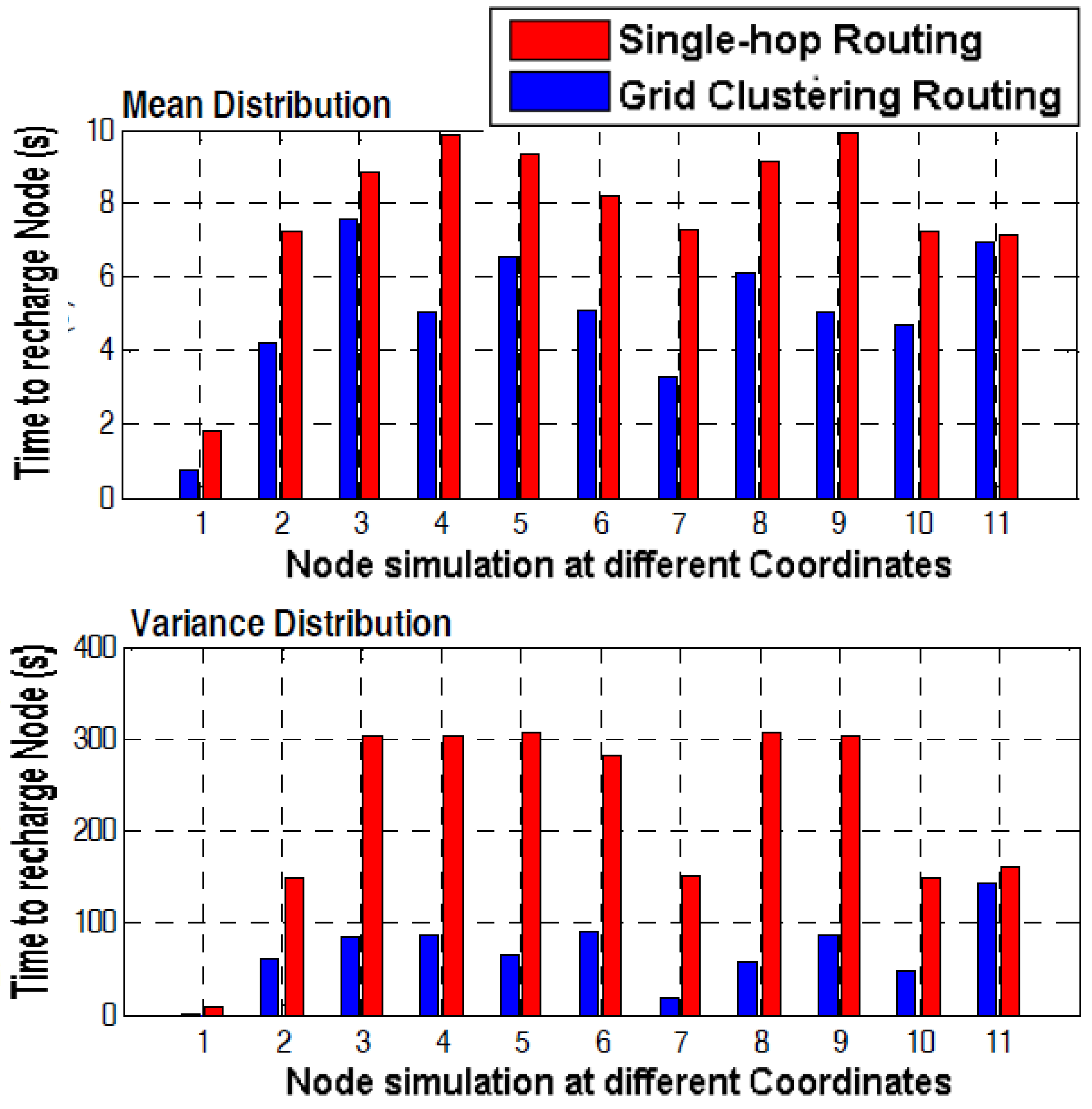
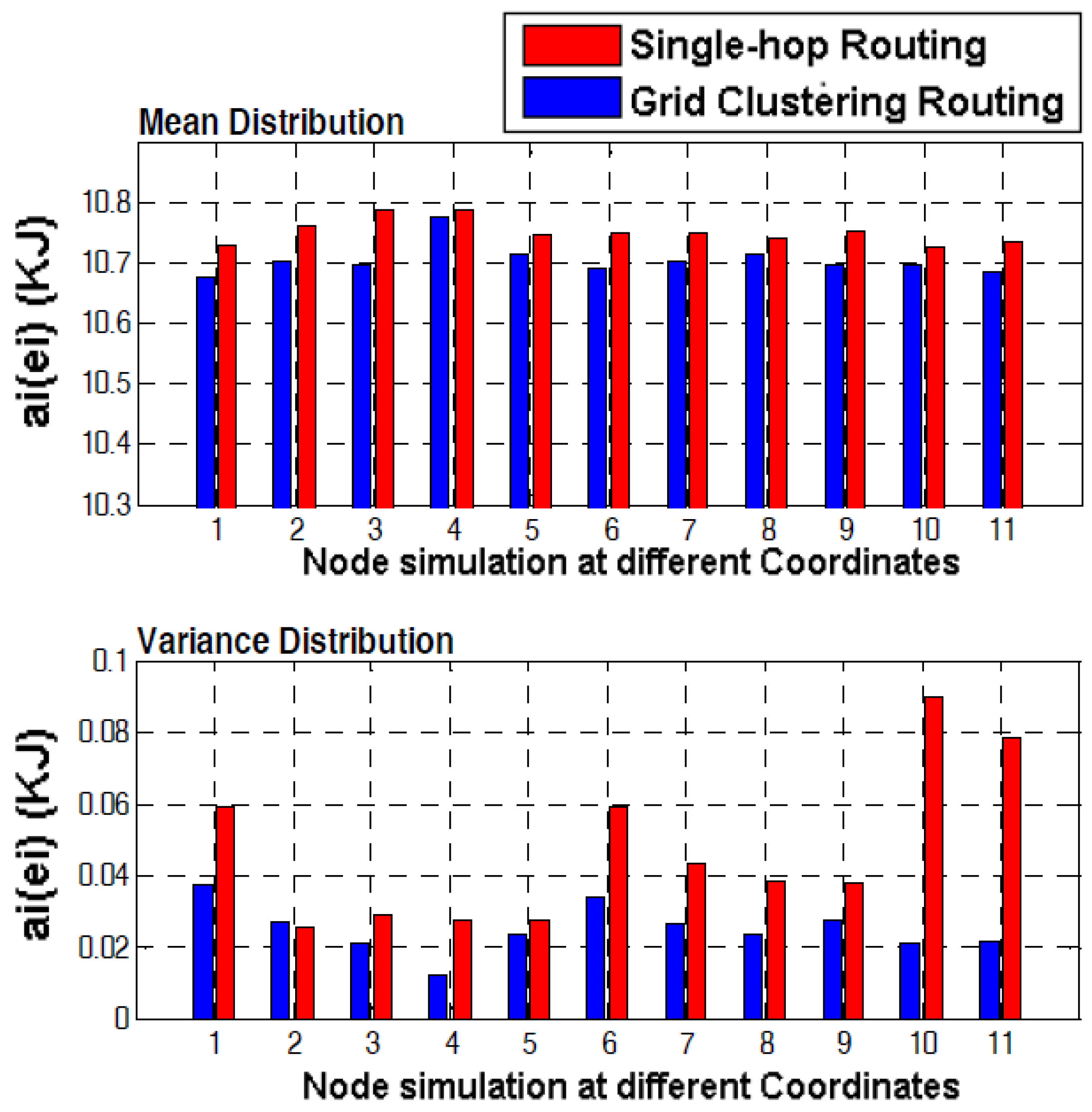
When the WPCD arrives at a node, there are two more factors involved, one is the time required to recharge the node, and the other is the minimal energy of each node in the WSN. Figure 10 is plotted to expose the mean and variance distribution of time needed to charge a node with the help of weighted grid-based routing and single-hop routing, as well. The mean and variance of the obtained simulated data has been calculated several times to check the reproducibility of the simulation. The rechargeable wireless network sustainability depends on the overall lifetime of small sensor nodes, which depends on the energy capacity of the node’s battery [42,43]. The high minimal energy of the node from applying the grid-based routing is shown in Figure 11. It is observed that the mean and variance distribution of the minimal energy of each node is also higher than the single-hop routing. The mean and variance distribution presented consistent results for the time to recharge the node and for minimal energy which is shown in Figure 10 and Figure 11, respectively.
6.3. Comparative Graphs
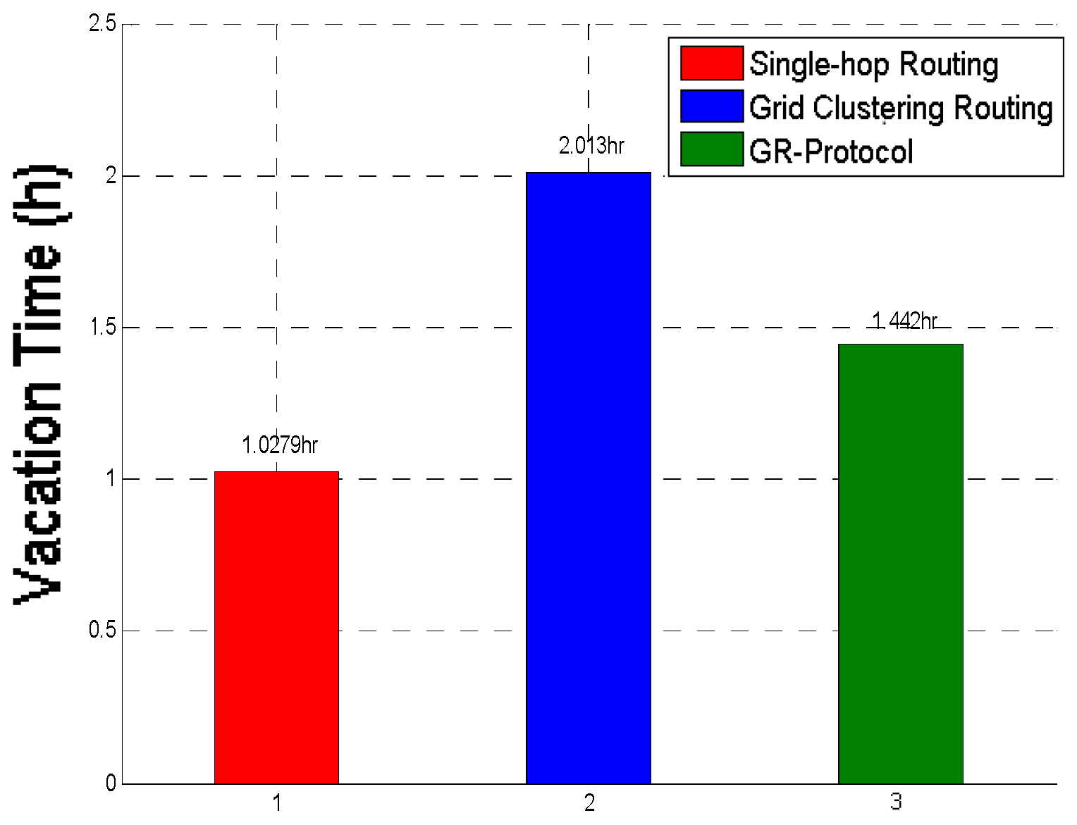
This section mainly refers to the comparison of the proposed method with single-hop routing and the existing GR-Protocol. Figure 12 shows the maximum vacation time. It is observed that our proposed mechanism displays almost 50% higher vacation time than that of single-hop routing. GR-Protocol divides the entire topology into several grids in a way that sensor nodes in the same grid are all serviced by the WPCD at the same time. So, this technique requires more time to recharge the sensor nodes for its one-to-many wireless recharging method. In our proposed method, the WPCD follows the shortest path algorithm to traverse the sensor nodes and at the same time, our energy conserving technique helps to keep enough energy for each sensor node. Thus, our solution outperforms the GR-Protocol. Energy management for a WSN is a basic issue that needs to be standardized. In our WSN, each node has some tasks (data transmission) to perform by utilizing its energy, while our objective is to perform those tasks with a minimum amount of energy.
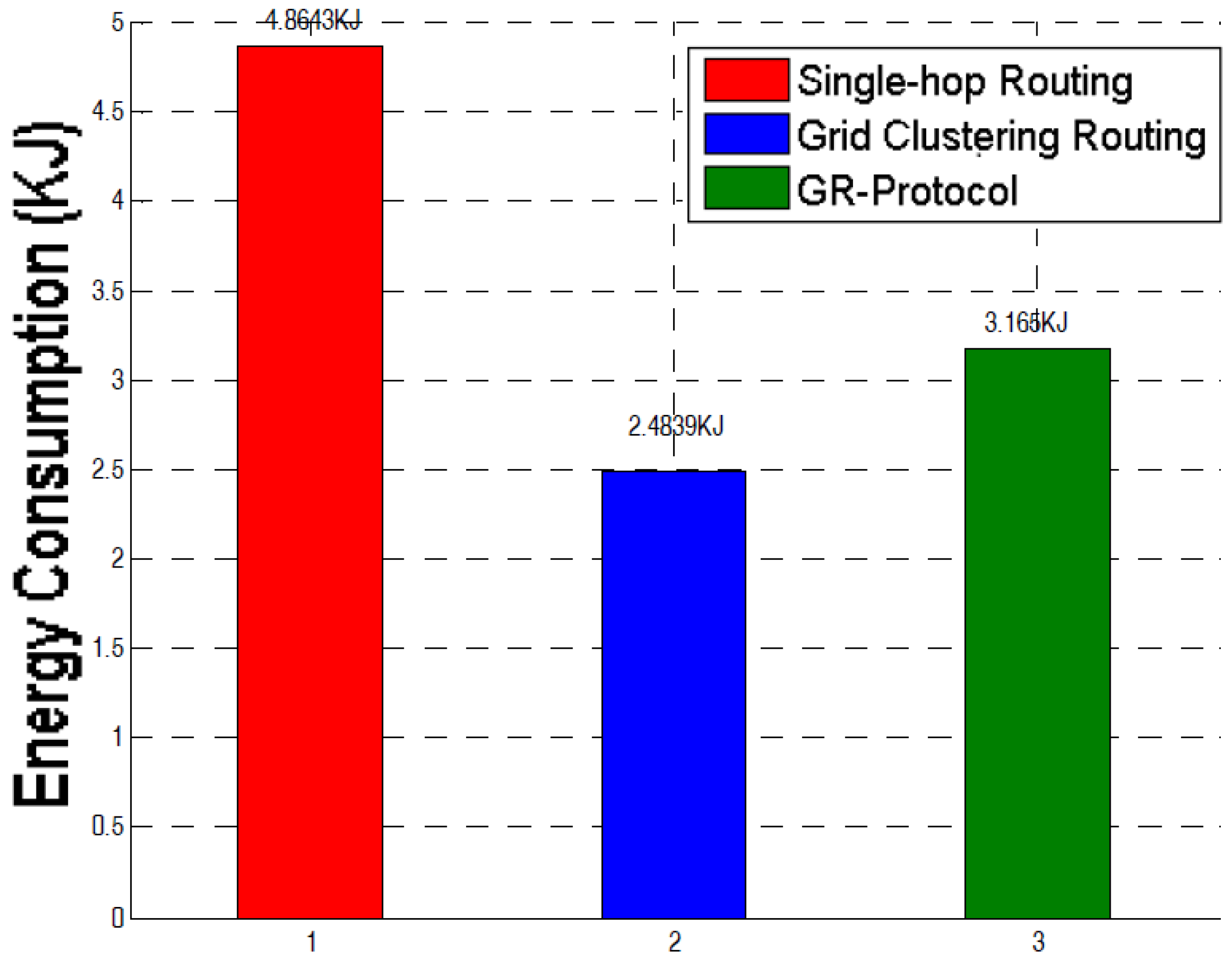
In the proposed approach, the clustering technique minimizes the transmission (data sending/receiving) energy of the sensor nodes. In single-hop routing, all the sensor nodes send the data to the base station directly with high transmission energy which gives the worst performance. GR-Protocol optimizes the traveling path of the WPCD only and does not consider the overall protocol for data routing in the WSN. Figure 13 shows that the proposed protocol outperforms both methods regarding energy consumption.
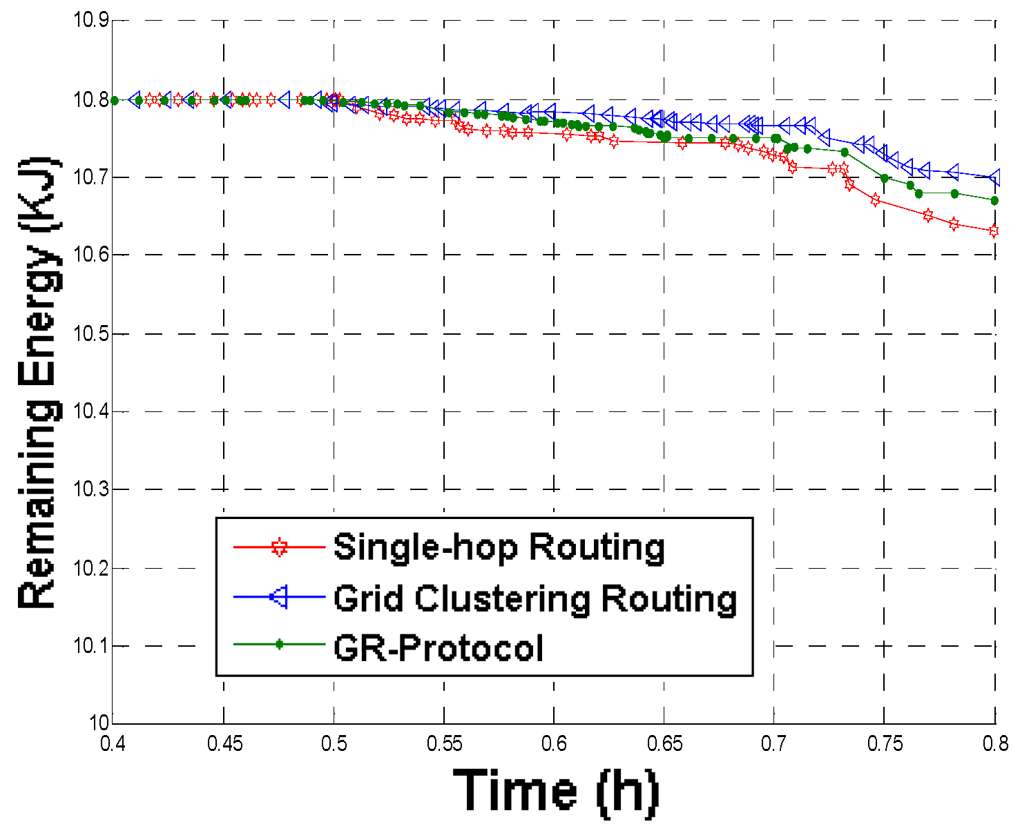
Once the WPCD completes its first cycle and returned to self-maintenance at the rest station, the next cycle needs to occur to make the WSN functional again. For this cycle, the remaining battery of each node plays a pivotal role. Suppose node 5 has a fifty percent charge remaining, then the WPCD spends less time to fully charge its battery. So, the proposed method manages the high remaining energy at each node. For the remaining energy, single-hop routing performs poorly. GR-Protocol shows moderate performance as its energy consumption level is better than single-hop and worse than our proposed method. This is shown in Figure 14.
Table 4 represents the overall time consumed, total distance and shortest traveling time by the WPCD in the renewable wireless network.
7. Conclusions and Future Work
This research finds that the loss of network persistence is the main drawback for WSNs, which can be improved with the use of renewable charge cycles and an efficient routing scheme. The suggested methodology results in maximizing the vacation time over the charge cycle time and optimizing the path for the WPCD with the help of a shortest path algorithm. The important properties of WSN are addressed, i.e., minimizing the recharge time, energy consumption, and maximizing the remaining energy of the node. The numerical and simulation results show that grid-based clustering is the much better energy conservation technique for extending the life of the WSN. The research model posits the best possible renewable cycle and grid clustering strategies and decides a better WSN layout for the efficiency of energy.
Probing deeper, the simulated results raise some points to be addressed in future work. One main point is the scalability, i.e., a wide area of the network should be taken for deployment of the WSN by reducing its phases. Another intention is to develop more economically feasible and energy saving strategies in the renewable charge cycle of a WSN. This strategy enables the WPCD to gather data from each node while charging the battery of that node concurrently. Further exploration is still required to investigate the issues mentioned above in the present work.
Acknowledgments
Our research work is funded by National Natural Science Foundation of China (No. 51208168), Natural Science Foundation of Hebei Province (No. 2016202341) and Natural Science Foundation (No. 13JCYBJC37700) of Tianjin as well.
Author Contributions
Nelofar Aslam and Kewen Xia conceived and designed the experiments; Nelofar Aslam performed the experiments; Nelofar Aslam and Muhammad Usman Hadi analyzed the data; Muhammad Tafseer Haider contributed analysis tools; and finally, Nelofar Aslam wrote the paper. All the authors have contributed substantially to the work reported.
Conflicts of Interest
The authors declare no conflicts of interest.
References
- Mahamuni, C. A military surveillance system based on wireless sensor networks with extended coverage life. In Proceedings of the 2016 International Conference on Global Trends in Signal Processing, Information Computing and Communication (ICGTSPICC), Jalgaon, India, 22–24 December 2016. [Google Scholar]
- Luo, H.; Wu, K.; Guo, Z.; Gu, L.; Ni, L. Ship Detection with Wireless Sensor Networks. IEEE Trans. Parallel Distrib. Syst. 2012, 23, 1336–1343. [Google Scholar] [CrossRef]
- Ramar, R.; Shanmugasundaram, R. Connected k-Coverage Topology Control for Area Monitoring in Wireless Sensor Networks. Wirel. Pers. Commun. 2015, 84, 1051–1067. [Google Scholar] [CrossRef]
- Yaakob, N.; Khalil, I. A Novel Congestion Avoidance Technique for Simultaneous Real-Time Medical Data Transmission. IEEE J. Biomed. Health Inform. 2016, 20, 669–681. [Google Scholar] [CrossRef] [PubMed]
- Risodkar, Y.; Pawar, A. A survey: Structural health monitoring of bridge using WSN. In Proceedings of the 2016 International Conference on Global Trends in Signal Processing, Information Computing and Communication (ICGTSPICC), Jalgaon, India, 22–24 December 2016. [Google Scholar]
- Lazarescu, M. Design of a WSN Platform for Long-Term Environmental Monitoring for IoT Applications. IEEE J. Emerg. Sel. Top. Circuits Syst. 2013, 3, 45–54. [Google Scholar] [CrossRef]
- Figueiredo, C.M.; Nakamura, E.F.; Ribas, A.D.; de Souza, T.R.; Barreto, R.S. Assessing the communication performance of wireless sensor networks in rainforests. In Proceedings of the 2009 2nd IFIP Wireless Days (WD), Paris, France, 15–17 December 2009; pp. 1–6. [Google Scholar]
- Lara-Cueva, R.; Gordillo, R.; Valencia, L.; Benitez, D. Determining the Main CSMA Parameters for Adequate Performance of WSN for Real-Time Volcano Monitoring System Applications. IEEE Sens. J. 2017, 17, 1493–1502. [Google Scholar] [CrossRef]
- Rotariu, C.; Bozomitu, R.; Cehan, V.; Pasarica, A.; Costin, H. A wireless sensor network for remote monitoring of bioimpedance. In Proceedings of the 2015 38th International Spring Seminar on Electronics Technology (ISSE), Eger, Hungary, 6–10 May 2015. [Google Scholar]
- Wang, P.; Hou, H.; He, X.; Wang, C.; Xu, T.; Li, Y. Survey on Application of Wireless Sensor Network in Smart grid. Procedia Comput. Sci. 2015, 52, 1212–1217. [Google Scholar] [CrossRef]
- Li, R.; Asaeda, H.; Li, J.; Fu, X. A Distributed Authentication and Authorization Scheme for In-Network Big Data Sharing. Digit. Commun. Netw. 2017. [Google Scholar] [CrossRef]
- Razzaque, M.; Dobson, S. Energy-Efficient Sensing in Wireless Sensor Networks Using Compressed Sensing. Sensors 2014, 14, 2822–2859. [Google Scholar] [CrossRef] [PubMed] [Green Version]
- Zaman, N.; Jung, L.T.; Yasin, M. Enhancing Energy Efficiency of Wireless Sensor Network through the Design of Energy Efficient Routing Protocol. J. Sens. 2016, 2016, 1–16. [Google Scholar] [CrossRef]
- Chang, J.H.; Tassiulas, L. Energy conserving routing in wireless ad-hoc networks. In Proceedings of the Nineteenth Annual Joint Conference of the IEEE Computer and Communications Societies, INFOCOM ’05, Tel Aviv, Israel, 26–30 March 2000; pp. 22–31. [Google Scholar]
- Li, Q.; Aslam, J.; Rus, D. Online power-aware routing in wireless Ad-hoc networks. In Proceedings of the 7th Annual International Conference on Mobile Computing and Networking, MobiCom ’01, Rome, Italy, 16–21 July 2001; pp. 97–107. [Google Scholar]
- Fan, K.-W.; Zheng, Z.; Sinha, P. Steady and fair rate allocation for rechargeable sensors in perpetual sensor networks. In Proceedings of the 6th ACM conference on Embedded network sensor systems, SenSys ’08, Raleigh, NC, USA, 5–7 November 2008; pp. 239–252. [Google Scholar]
- Meninger, S.; Mur-Miranda, J.; Amirtharajah, R.; Chandrakasan, A.; Lang, J. Vibration-to-electric energy conversion. IEEE Trans. VLSI Syst. 2001, 9, 64–76. [Google Scholar] [CrossRef]
- Kansal, A.; Potter, D.; Srivastava, M.B. Performance aware tasking for environmentally powered sensor networks. In Proceedings of the Joint International Conference on Measurement and Modeling of Computer Systems—SIGMETRICS 2004/Performance 2004, New York, NY, USA, 10–14 June 2004. [Google Scholar]
- Park, C.; Chou, P. AmbiMax: Autonomous Energy Harvesting Platform for Multi-Supply Wireless Sensor Nodes. In Proceedings of the 2006 3rd Annual IEEE Communications Society on Sensor and Ad Hoc Communications and Networks, Reston, VA, USA, 25–28 September 2006. [Google Scholar]
- Tong, B.; Li, Z.; Wang, G.; Zhang, W. On-Demand Node Reclamation and Replacement for Guaranteed Area Coverage in Long-Lived Sensor Networks. In Lecture Notes of the Institute for Computer Sciences, Social Informatics and Telecommunications Engineering; Quality of Service in Heterogeneous Networks; Springer: Berlin/Heidelberg, Germany, 2009; pp. 148–166. [Google Scholar]
- Tong, B.; Wang, G.; Zhang, W.; Wang, C. Node Reclamation and Replacement for Long-lived Sensor Networks. In Proceedings of the 2009 6th Annual IEEE Communications Society Conference on Sensor, Mesh and Ad Hoc Communications and Networks, Rome, Italy, 22–26 June 2009. [Google Scholar]
- Yang, J.; Ozel, O.; Ulukus, S. Broadcasting with an Energy Harvesting Rechargeable Transmitter. IEEE Trans. Wirel. Commun. 2012, 11, 571–583. [Google Scholar] [CrossRef]
- Klues, K.; Hackmann, G.; Chipara, O.; Lu, C. A component-based architecture for power-efficient media access control in wireless sensor networks. In Proceedings of the 5th International Conference on Embedded Networked Sensor Systems—SenSys ’07, Sydney, Australia, 6–9 November 2007. [Google Scholar]
- Yang, Y.; Wang, C. Wireless Rechargeable Sensor Networks; SpringerBriefs in Electrical and Computer Engineering; Springer: Cham, Switzerland, 2015. [Google Scholar]
- Kurs, A.; Karalis, A.; Moffatt, R.; Joannopoulos, J.D.; Fisher, P.; Soljacic, M. Wireless Power Transfer via Strongly Coupled Magnetic Resonances. Science 2007, 317, 83–86. [Google Scholar] [CrossRef] [PubMed]
- André, K.; Moffatt, R.; Marin, S. Simultaneous mid-range power transfer to multiple devices. Appl. Phys. Lett. 2010, 96, 044102. [Google Scholar]
- Hassan, M.; Zawawi, A. Wireless power transfer (Wireless lighting). In Proceedings of the 2015 5th International Conference on Information & Communication Technology and Accessibility (ICTA), Marrakech, Morocco, 21–23 December 2015. [Google Scholar]
- Chen, S.-H.; Cheng, Y.-C.; Lee, C.-H.; Wang, S.-P.; Chen, H.-Y.; Chen, T.-Y.; Wei, H.-W.; Shih, W.-K. Extending sensor network lifetime via wireless charging vehicle with an efficient routing protocol. In Proceedings of the SoutheastCon 2016, Norfolk, VA, USA, 30 March–3 April 2016. [Google Scholar]
- Rahimi, M.; Shah, H.; Sukhatme, G.; Heideman, J.; Estrin, D. Studying the feasibility of energy harvesting in a mobile sensor network. In Proceedings of the 2003 IEEE International Conference on Robotics and Automation (Cat. No. 03CH37422), Taipei, Taiwan, 14–19 September 2003. [Google Scholar]
- Shi, Y.; Xie, L.; Hou, Y.T.; Sherali, H.D. On renewable sensor networks with wireless energy transfer. In Proceedings of the IEEE INFOCOM 2011, Shanghai, China, 10–15 April 2011. [Google Scholar]
- Shi, L.; Han, J.; Han, D.; Ding, X.; Wei, Z. The dynamic routing algorithm for renewable wireless sensor networks with wireless power transfer. Comput. Netw. 2014, 74, 34–52. [Google Scholar] [CrossRef]
- Fu, L.; He, L.; Cheng, P.; Gu, Y.; Pan, J.; Chen, J. ESync: Energy Synchronized Mobile Charging in Rechargeable Wireless Sensor Networks. IEEE Trans. Veh. Technol. 2015, 65, 7415–7431. [Google Scholar] [CrossRef]
- Li, S.; Mi, C.C. Wireless Power Transfer for Electric Vehicle Applications. IEEE J. Emerg. Sel. Top. Power Electron. 2015, 3, 4–17. [Google Scholar]
- Chen, S.-H.; Chen, T.-Y.; Cheng, Y.-C.; Wei, H.-W.; Hsu, T.-S.; Shih, W.-K. Developing a user-friendly sensor network simulator to imitate wireless charging vehicle behaviors. In Proceedings of the 2016 International Conference on Computing, Networking and Communications (ICNC), Kauai, HI, USA, 15–18 February 2016. [Google Scholar]
- WiPower | Qualcomm. 2017. Available online: https://www.qualcomm.com/products/wipower (accessed on 5 August 2017).
- Xie, L.; Shi, Y.; Hou, Y.T.; Lou, W.; Sherali, H.D.; Midkiff, S.F. On renewable sensor networks with wireless energy transfer: The multi-node case. In Proceedings of the 2012 9th Annual IEEE Communications Society Conference on Sensor, Mesh and Ad Hoc Communications and Networks (SECON), Seoul, Korea, 18–21 June 2012. [Google Scholar]
- Kumar, K.S.; Amutha, R. An Algorithm for Energy Efficient Cooperative Communication in Wireless Sensor Networks. KSII Trans. Internet Inf. Syst. 2016, 10, 3080–3099. [Google Scholar]
- Zhuang, Y.; Pan, J.; Wu, G. Energy-optimal grid-based clustering in wireless microsensor networks with data aggregation. Int. J. Parallel Emergent Distrib. Syst. 2010, 25, 531–550. [Google Scholar] [CrossRef]
- Nakade, V.; Chavhan, N. Review on DRINA: An Energy Efficient Routing Approach for Wireless Sensor Networks. In Proceedings of the 2015 Fifth International Conference on Communication Systems and Network Technologies, Gwalior, India, 4–6 April 2015. [Google Scholar]
- MATLAB R2015a Free Download. Download Latest Free Software. [Online]. Available online: https://www.mathworks.com/products.html?s_tid=gn_ps (accessed on 1 September 2016).
- Reddy, T.B. Linden’s Handbook of Batteries, 4th ed.; McGraw-Hill: New York, NY, USA, 2011. [Google Scholar]
- Rout, R.R.; Krishna, M.S.; Gupta, S. Markov Decision Process-Based Switching Algorithm for Sustainable Rechargeable Wireless Sensor Networks. IEEE Sens. J. 2016, 16, 2788–2797. [Google Scholar] [CrossRef]
- Sun, P.; Li, G.; Wang, F. An Adaptive Back-Off Mechanism for Wireless Sensor Networks. Future Internet 2017, 9, 19. [Google Scholar] [CrossRef]
Figure 1.
A sketch of a sensor network with a wireless portable charging device (WPCD).
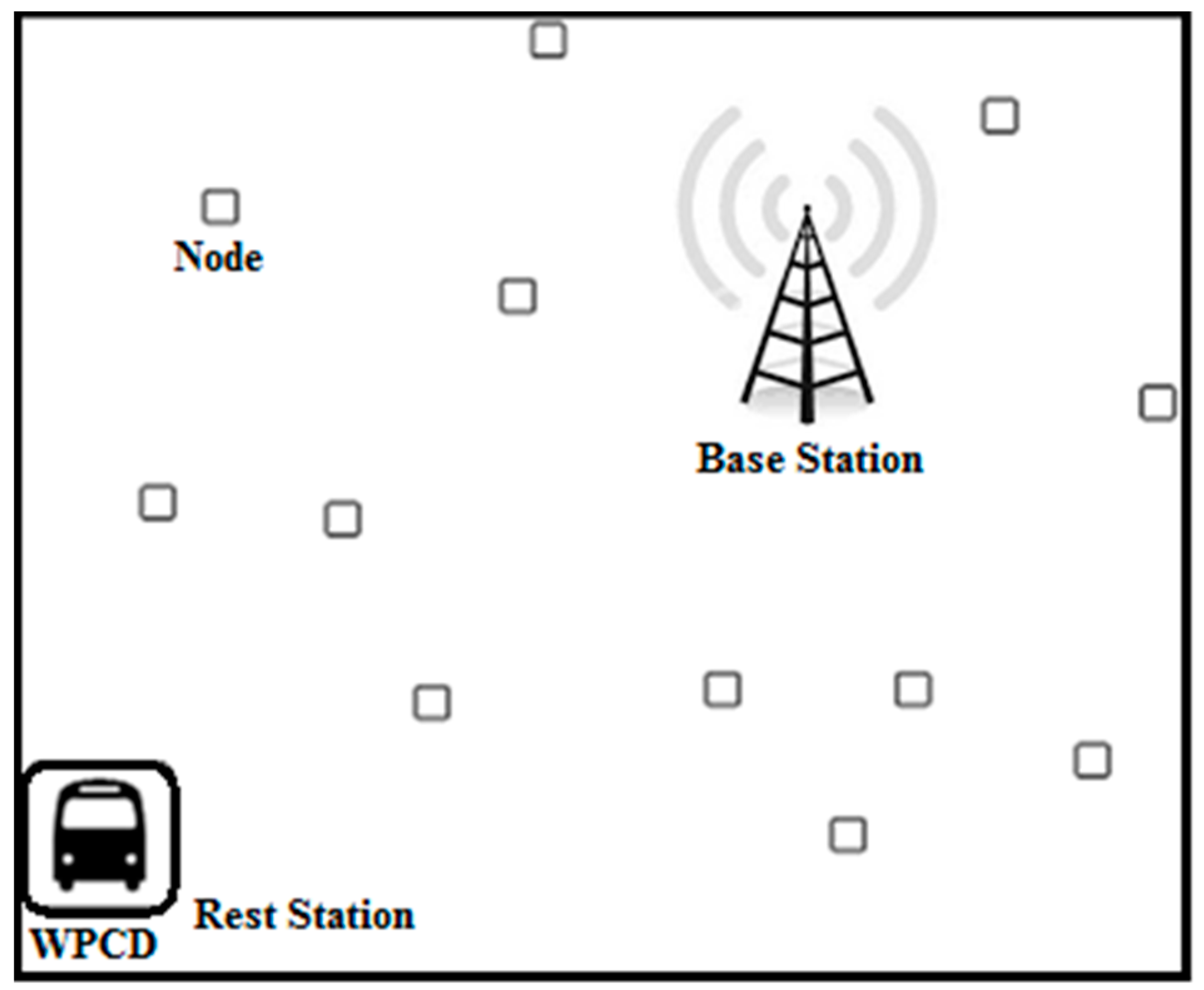
Figure 2.
Weighted grid clustering routing design diagram.

Figure 3.
Roles of nodes in the clustered environment.

Figure 4.
Node’s status (Wu) at different simulations for being a cluster head (CH).
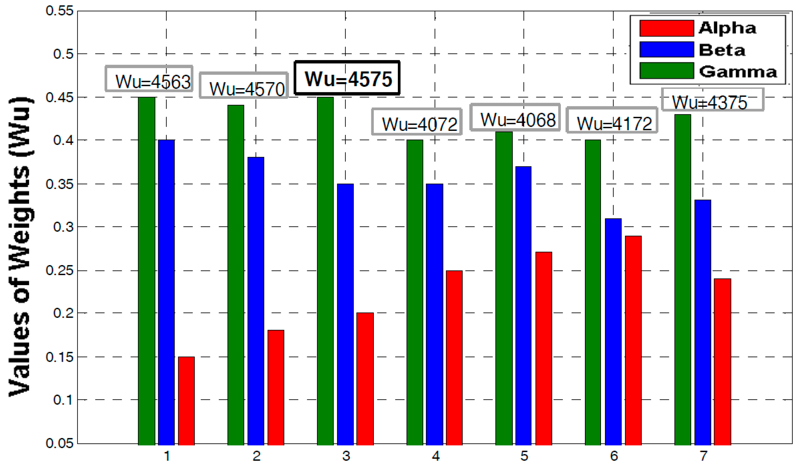
Figure 5.
Randomly deployed node in the wireless sensor network (WSN).
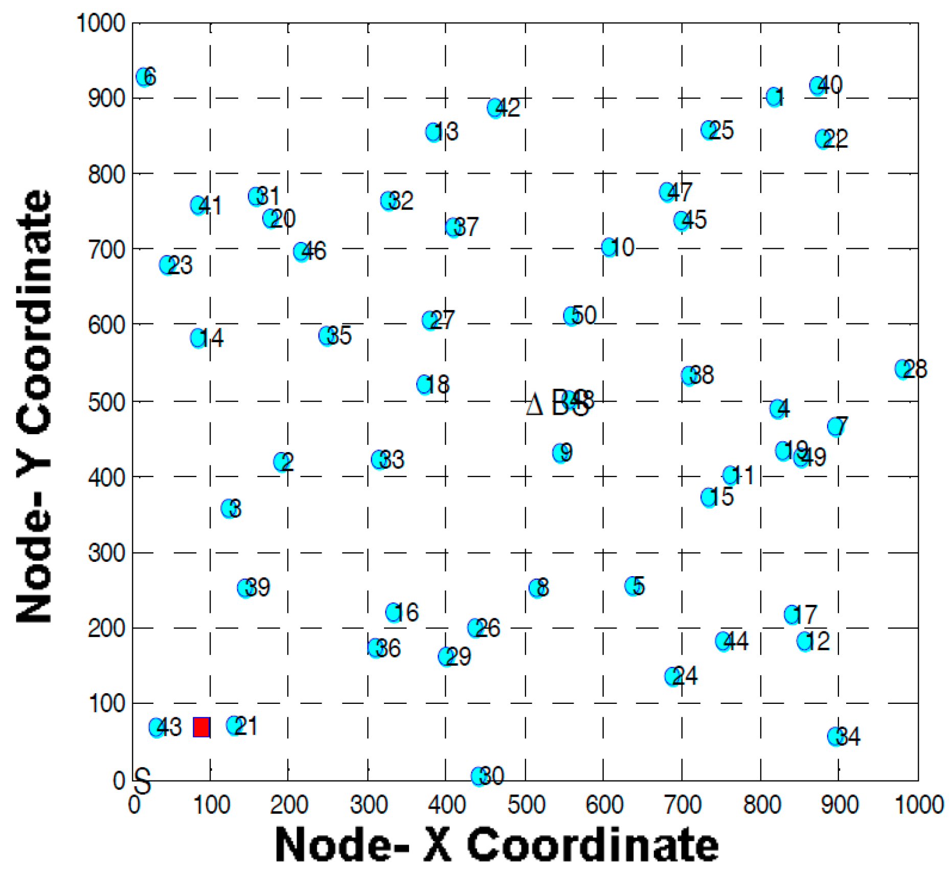
Figure 6.
Shortest path measurement.
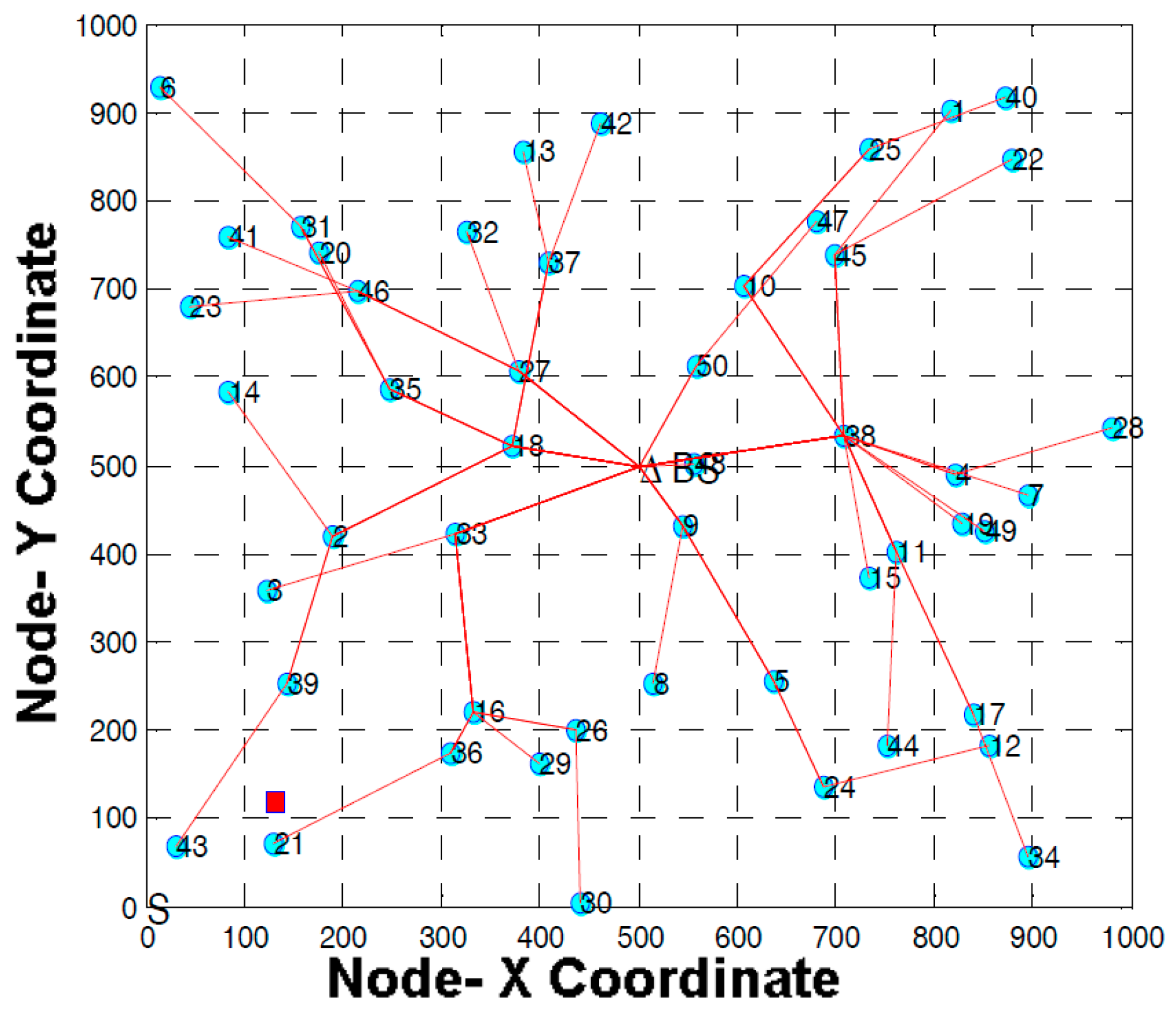
Figure 7.
Grid clustering routing.

Figure 8.
Data sending rate of the network.

Figure 9.
Arriving time of WPCD at each node.

Figure 10.
Time needed to recharge the specific node.

Figure 11.
Minimal energy of each node.

Figure 12.
Comparative vacation times of the WPCD.

Figure 13.
Energy consumption of 50 deployed nodes.

Figure 14.
Remaining energy after first charge cycle.


Table 1.
Notations for the entire network model.
| Notation | Detail Description of the Notations |
|---|---|
| WPCD | wireless portable charging device |
| RS | rest station |
| BS | base station |
| N | number of nodes in the wireless sensor networks |
| P | path of travel for WPCD |
| Ƥ | the whole set of traveling path for WPCD |
| ACK | route formation acknowledgment message |
| ρ | the coefficient of energy consumption for receiving the data |
| Tm | the whole set of time instances in considering m phase |
| U | the full transfer rate of WPCD |
| V | revolving speed of WPCD |
| ai | time to approach node i by WPCD in the first charge cycle |
| Cij or CiB | energy consumption coefficient for sending data from node i to j and base station alternatively |
| Dij | located distance between node i and j |
| Dp | moving distance for the prescribed path P |
| DTSP | shortest traveled distance in a charge cycle |
| Emax | the maximum energy of a node’s battery |
| Emin | the minimum energy of a node’s battery |
| ei(t) | the energy of sensor node at time t |
| gij(t) or giB(t) | the coefficient for flow rate from node i to j base station respectively |
| Ri | the rate of gathering data by monitoring the environment |
| Ui | power transfer rate at node i in the first charge cycle |
| πi | ith node visited by the WPCD |
| τ | complete time spent by the WPCD in a charge cycle |
| τi | time used by the WPCD to charge the battery of node i |
| τ0 | a time when WPCD is not transferring power to any node |
| τvac | vacation time (time for WPCD to be charge itself) |
| τp | time to travel of WPCD for a path P |
| τTSP | minimum moving time of WPCD in the charge cycle |
Table 2.
Simulation parameters.
| Parameters | Assumed Values |
|---|---|
| Number of nodes | 50 |
| Length | 1000 m |
| Width | 1000 m |
| Emax | 10,800 J |
| Emin | 540 J |
| ρ | 5 × 10⁻⁸ J/b |
| Location of BS | [500, 500] m |
| Location of WPCD | [0,0] |
| Speed of WPCD | 5 m/s |
| U | 5 W |
| Antenna | Omni-directional |
| Path Loss | Log Normal Shadowing |
| Routing | Grid-based clustering, Single-hop, GR-Protocol |
| Simulation run time | Almost 1 h |
| Communication radius | 100 m |
| Voltage of battery (NiMH) | 1.2 V |
| Electricity quantity of battery (NiMH) | 2.5 Ah |
Table 3.
Each node performance.
| Node | Node Location (m) (x, y) | Arriving Time of WPCD (s) | Node’s Minimal Energy ei(ai) kj | Node Location (m) (x, y) | Arriving Time of WPCD (s) | Node’s Minimal Energy ei(ai) kj |
|---|---|---|---|---|---|---|
| Single-hop Routing | Single-hop Routing | Single-hop Routing | Grid Clustering Routing | Grid Clustering Routing | Grid Clustering Routing | |
| 1 | (816.9, 901.8) | 1757.1 | 10.6 | (816.9, 901.8) | 1498.9 | 10.8 |
| 2 | (189.5, 419.5) | 1821.9 | 10.5 | (189.5, 419.5) | 1515.4 | 10.8 |
| 3 | (123.7, 358.1) | 1849.2 | 10.7 | (123.7, 358.1) | 1547.1 | 10.8 |
| 4 | (821.0, 489.0) | 1873.9 | 10.7 | (821.0, 489.0) | 1576.1 | 10.8 |
| 5 | (637.9, 256.0) | 1894.8 | 10.6 | (637.9, 256.0) | 1605.5 | 10.8 |
| 6 | (16.1, 929.2) | 1908.7 | 10.7 | (16.1, 929.2) | 1635.7 | 10.8 |
| 7 | (896.0, 466.7) | 1951.8 | 10.7 | (896.0, 466.7) | 1650.4 | 10.8 |
| 8 | (515.3, 254.0) | 1969.8 | 10.7 | (515.3, 254.0) | 1662.1 | 10.8 |
| 9 | (544.5, 431.2) | 1995.9 | 10.7 | (544.5, 431.2) | 1674.4 | 10.8 |
| 10 | (606.4, 702.5) | 2014.4 | 10.7 | (606.4, 702.5) | 1698.2 | 10.8 |
| 11 | (760.4, 402.3) | 2056.3 | 10.7 | (760.4, 402.3) | 1747.4 | 10.8 |
| 12 | (855.3, 181.8) | 2098.6 | 10.4 | (855.3, 181.8) | 1789.6 | 10.8 |
| 13 | (382.9, 856.2) | 2134.0 | 10.4 | (382.9, 856.2) | 1799.6 | 10.8 |
| 14 | (84.6, 584.2) | 2146.2 | 10.7 | (84.6, 584.2) | 1803.3 | 10.8 |
| 15 | (733.9, 373.5) | 2159.6 | 10.7 | (733.9, 373.5) | 1809.5 | 10.8 |
| 16 | (733.9, 373.6) | 2175.5 | 10.7 | (733.9, 373.6) | 1838.0 | 10.8 |
| 17 | (839.7, 219.0) | 2229.5 | 10.5 | (839.7, 219.0) | 1874.3 | 10.8 |
| 18 | (371.7, 522.2) | 2250.5 | 10.7 | (371.7, 522.2) | 1897.5 | 10.7 |
| 19 | (828.2, 433.4) | 2275.9 | 10.7 | (828.2, 433.4) | 1919.7 | 10.8 |
| 20 | (176.5, 741.3) | 2303.5 | 10.7 | (176.5, 741.3) | 1939.6 | 10.8 |
Table 4.
Entire simulation results for a wireless rechargeable network.
| Single-Hop Routing | Grid Clustering Routing | |
|---|---|---|
| Total Distance covered by WPCD | 6502.826120 (m) | 6761.404616 (m) |
| Traveling Time for WPCD by Physical Path P | 1300.565224 (s) | 1352.280923 (s) |
| Overall Time consumed in the renewable charge cycle | 1666.658984 (s) | 1393.098968 (s) |
© 2017 by the authors. Licensee MDPI, Basel, Switzerland. This article is an open access article distributed under the terms and conditions of the Creative Commons Attribution (CC BY) license (http://creativecommons.org/licenses/by/4.0/).
Share and Cite
MDPI and ACS Style
Aslam, N.; Xia, K.; Haider, M.T.; Hadi, M.U. Energy-Aware Adaptive Weighted Grid Clustering Algorithm for Renewable Wireless Sensor Networks. Future Internet 2017, 9, 54. https://doi.org/10.3390/fi9040054
AMA Style
Aslam N, Xia K, Haider MT, Hadi MU. Energy-Aware Adaptive Weighted Grid Clustering Algorithm for Renewable Wireless Sensor Networks. Future Internet. 2017; 9(4):54. https://doi.org/10.3390/fi9040054
Chicago/Turabian StyleAslam, Nelofar, Kewen Xia, Muhammad Tafseer Haider, and Muhammad Usman Hadi. 2017. "Energy-Aware Adaptive Weighted Grid Clustering Algorithm for Renewable Wireless Sensor Networks" Future Internet 9, no. 4: 54. https://doi.org/10.3390/fi9040054
Note that from the first issue of 2016, this journal uses article numbers instead of page numbers. See further details here.