Analyzing Land Cover Change and Urban Growth Trajectories of the Mega-Urban Region of Dhaka Using Remotely Sensed Data and an Ensemble Classifier

Department of Geography, University of Florida; Gainesville, FL 32611, USA
*
Author to whom correspondence should be addressed.
Sustainability 2018, 10(1), 10; https://doi.org/10.3390/su10010010
Submission received: 29 November 2017
/
Revised: 19 December 2017
/
Accepted: 19 December 2017
/
Published: 21 December 2017
(This article belongs to the Special Issue Sustainability in an Urbanizing World: The Role of People)
Abstract
:Accurate information on, and human interpretation of, urban land cover using satellite-derived sensor imagery is critical given the intricate nature and niches of socioeconomic, demographic, and environmental factors occurring at multiple temporal and spatial scales. Detailed knowledge of urban land and their changing pattern over time periods associated with ecological risk is, however, required for the best use of critical land and its environmental resources. Interest in this topic has increased recently, driven by a surge in the use of open-source computing software, satellite-derived imagery, and improved classification algorithms. Using the machine learning algorithm Random Forest, combined with multi-date Landsat imagery, we classified eight periods of land cover maps with up-to-date spatial and temporal information of urban land between the period of 1972 and 2015 for the mega-urban region of greater Dhaka in Bangladesh. Random Forest—a non-parametric ensemble classifier—has shown a quantum increase in satellite-derived image classification accuracy due to its outperformance over traditional approaches, e.g., Maximum Likelihood. Employing Random Forest as an image classification approach for this study with independent cross-validation techniques, we obtained high classification accuracy, user and producer accuracy. Our overall classification accuracy ranges were between 85% and 97% with kappa values between 0.81 and 0.94. The area statistics derived from the thematic land cover map show that the built-up area in the 43-year study period expanded quickly, from 35 km2 in 1972 to 378 km2 in 2015, with a net increase rate of approximately 980% and an average annual growth rate of 6%. This growth rate, however, was higher in peripheral areas, with a 2903% increase and an annual expansion rate of 8%, compared to a 460% increase with an annual growth rate of 4% in the core city area (Dhaka City Corporation). This huge urban expansion took place in the north, northwest, and southwest regions of Dhaka, transforming areas that were previously agricultural land, vegetation cover, wetland, and water bodies. The main factors driving the city towards northern corridors include flood-free higher land, the availability of a transportation network, and the agglomeration of manufacturing-based employment centers. The resulting thematic map and spatial information produced from this study therefore serve to facilitate a detailed understanding of urban growth dynamics and land cover change patterns in the mega-urban region of Dhaka, Bangladesh.
1. Introduction
Although the overwhelming majority of Bangladesh’s population lives in rural settings with a low level of urbanization compared to other Asian countries (currently 34%), the megacity of Dhaka has experienced massive urbanization in recent years, which sharply contrasts with the rate of urbanization in other nations. The population of Dhaka, for example, rapidly inflated from nearly 1 million people in 1972 to 17 million or more in 2015 [1,2,3], making it one of the most densely inhabited and most quickly urbanized cities in the world [4]. Various estimates suggest that if the current trend of population growth continues, together with the ever-increasing economic growth and industrialization that is expected to occur over the next 10–15 years, Dhaka will emerge as the sixth-largest urban cluster on the planet [3]. The Dhaka mega-urban center is projected to reach an annual population growth rate of 2.98% by 2030, with the total population in the city territory surpassing 27.37 million by this time [1,3], and exceeding the growth rate of other major urban centers such as Beijing, Shanghai, and Mexico City. This immense and swift urbanization driven by population growth in Dhaka is primarily inflated by a great influx of rural migrants. Rural dwellers immigrate to the urban center either looking for work in a booming industrial sector (i.e., such as readymade garments around the city) [5] or to avail themselves of civic facilities such as health care clinics, education, and so on. Such growth has also resulted from the increasing frequency of natural disasters like floods, erosion, increasing salinization, and concomitant loss of agricultural productivity in the surrounding countryside, which has previously caused large-scale rural-to-urban migration. The current urbanization pattern with its fast and uncontrolled expansion, has, however, put Dhaka’s critical environment, ecology, and land resources at further risk, especially with the presence of highly eco-sensitive wetland areas in close proximity to the city [6]. For example, water bodies and wetlands surrounding Dhaka are facing destruction as these are being filled up to construct multi-storied buildings and other real estate developments. Coupled with an unbearable traffic gridlock, high pollution levels, and insufficient infrastructure and housing development [2], this ranks Dhaka as one of the least livable cities on Earth [7].
There have been overwhelming indications that such rapid urbanization with increasing anthropogenic activities driven by population growth has been the major driver of changing land cover and the resultant escalated impact on global climate change [8], with other long-lasting effects on many biophysical processes [9] Such unplanned urbanization and commensurate land cover change is the primary cause of habitat transformation [10,11], losses of biodiversity, and the breakdown of ecosystem services [10]. Noticeable impacts on the adjacent environment of urbanized land cover include broad exploitation of productive agricultural land [11,12], wildlife habitat degradation and isolation [9], hydrological cycle disruption [13], and degradation of green cover patches [14]. Furthermore, urbanization destroys soil productivity by changing the structure and function of agricultural landscapes [15,16], causing serious threats to fresh food production while simultaneously increasing the risk to long-term food security in the region and beyond [11].
The megacity of Dhaka shelters large proportions of the urban population and is responsible for a major share of the country’s economic activities as well as the consumption of food and natural resources. The city is the major engine of Bangladesh’s economic growth, which yields about one-third of the country’s total GDP [17]. Due to its massive population concentrations and rapid development dynamics, Dhaka is gaining increasing importance as an economic, political, and administrative hub for the whole nation. Despite its rapid population increase and significant urban expansion, the volume of scientific research and analysis of the urbanization trends, patterns, and processes of Dhaka in relation to their spatial and temporal context has yet to be produce conclusions. Earlier studies carried out by Dewan et al. (2009) [18] and Ahmed et al. (2015) [19] aimed to explain land cover change in Dhaka; however, their attempts were limited in terms of aerial extension, temporal frequencies, and available methodology. In addition, accurate information on the physical dimensions of urban areas is often confusing and difficult to obtain.
Given the rapid rate of urban expansion with high inter- and intra-annual variability of land use practices in developing countries like Bangladesh, a higher frequency and a longer temporal sequence of urban growth analysis is crucial, such that decadal changes are no longer enough. Rather, a much higher frequency of analysis is preferred. Such consistent monitoring enables concerned authorities to have a clear picture of the current state of various land use types, and the physical direction and the complexity of their development dynamics over time in response to evolving economic, social, and biophysical conditions. Thus, a better understanding of land and environmental resources and their changing patterns is crucial for a sustainable urban future for Dhaka.
As remote sensing represents a major source of current and historical urban information by providing spatially consistent coverage of large areas with fine spatial resolution and temporal frequencies [20], the aim of this study is, therefore, to quantify the full continuum of urban growth in Dhaka using open-source Landsat imagery. Using the ensemble classifier Random Forest with multi-date remote sensing imagery, we studied land cover change and urban expansion of the greater Dhaka for the period of 1972 to 2015. The land cover map and spatial metrics generated from this study may serve as a valuable tool for planners who need to better understand and more accurately characterize urban processes and territorial planning regarding urban growth in Dhaka’s region.
2. Materials and Methods
2.1. Study Area
Dhaka has the unique position of being at once the oldest, historically largest, and most centrally located city in Bangladesh (23.3–24.6° N and 90.1–90.3° E) (Figure 1). The current study area is a polycentric urbanized area, comprising a number of cities and growth centers that are physically contiguous with and relate to one another through population growth, economic activities, and physically connections (developed road networks and urban expansion). Dhaka and neighboring areas are witnessing a surge of industrial and economic activities and has become an attractive destination for direct foreign investment in Bangladesh. It is a powerful engine of economic growth, providing important economic, social, and cultural opportunities for the entire nation. The total aerial expansion of this mega-urban region as selected for this study is 1528 km2, which is called the Detailed Urban Planning Area of Greater Dhaka (DAP).
Historically, the city witnessed a lot of different rulers and kingdoms, which led to its development as a widely-connected urban center. In the 7th to 8th centuries, Dhaka was under the Buddhist kingdom, then controlled by Hindu rulers. From 1299 to 1608 the city was governed by Turks and Pathans, and then dominated by Mughals beginning in 1608 [21]. From the beginning of the 17th century Dhaka was governed by a succession of European settlers, first by the Portuguese, then the Dutch, French, and later the English colonial powers [22].
Originally Dhaka City was a small town lying between the rivers Buriganga in the south and Dulai Khal in north, with its center near the present Bangla Bazar [23]. Later the city expanded northwards from the banks of the Buriganga River due to the physical constraints imposed by vast swampy areas to the east and west of the city. This barrier still exists but is no longer as effective as in the past since much of this swampy land has already been filled in or is targeted for future urban development and infilling by land developers, co-operative societies, or individuals. As a result, while the city is still expanding northwards, it is now also experiencing growth in all directions and mostly in chaotic and unplanned ways. The 400-year-old city first came within the framework of planning in 1840 with the formation of a municipal committee [24]. A more formal organization of urban development was initiated in 1959 with the adoption of a master plan [23]. Dhaka was first electrified in 1878 and connected by railway with the southeast-neighboring township of Naryanganj in 1885.
Dhaka City and its surrounding areas comprise six municipalities, Kadamrasul, Gazipur, Naryanganj, Sidirganj, Savar, and Tongi, and a number of connecting small urban areas. They are physically contiguous, and have grown into one of the world’s largest megacities, with a very rapid rate of urban expansion. There are five major river systems rolling across the megacity, i.e., the Buriganga-Dhaleshwari to the south, Bansi-Dhaleshwari to the west, Turag Rivers to the North-West, Tongi Khal to the North, and the Shitallakhya-Balu to the east and southeast. These rivers have been the most important means of travel and communication for a long period. Dhaka and its neighboring areas are composed of alluvial terraces of the southern part of the Pleistocene uplands known as the Madhupur tract and low-lying areas around the confluence of the Meghna and Lakhya rivers.
Geomorphic classifications reveal that a relatively young floodplain constitutes the largest area, followed by the higher terraces of the Pleistocene period. Low-lying swamps and marshes located in and around the city are examples of other major geomorphic features.
The elevation in the area ranges from 0 to 24 m above mean sea level. Except for the Pleistocene terraces on the northern edge, 17% of the land is 0–5 m above mean sea level, which accounts for 250 km2 of the total area. In addition, around 21% of the land is 6–7 m (314 km2), and the rest (53%) of the land is 9–24 m above the mean sea level. Dhaka enjoys a fairly equitable tropical monsoon climate, with an annual average temperature of 25 °C (77° F) and monthly means varying between 18 °C (64° F) in January and 29 °C (84° F) in August. Annual rainfall of Dhaka City varies from 1169 to 3028 mm and the annual average rainfall of 2076 mm [25]. Nearly 80% of the rainfall occurs during the monsoon season, which lasts from May to the end of September.
2.2. Data and Processing
This study uses a series of Landsat imagery, geospatial information, and multilayer census data in addition to fieldwork and survey data. Considering the local climate patterns, especially the effect of the monsoon on image spectral signatures and landscape configuration across the study area, we downloaded eight periods of cloud-free Landsat images captured in the dry season between December and January for the following years: MSS 1972, 1980, TM 1990, 1995, 2005, 2010, ETM+ 2000, and OLI-TIRS 2015. Along with Landsat data, a supplementary night light imagery, OLS (Operational Line-scan System) sensor, 1 km2 spatial resolution, version 4, Defense Meteorological Satellite Program/Operational Linesca System (DMSP-OLS) Nighttime Lights composite images were downloaded from NOAA (https://www.ngdc.noaa.gov/). Since urban areas or developed regions reveal higher light reflectance during the night time [26], this DMSP-OLS night light signature is believed to be an important driver in our regression-based model calibration. As DMSP-OLS data are only available from 1992 to 2013, spectral signature of these imagery for 1992, 1995, 2000, 2005, 2010, and 2013 were used for model calibration for the years 1990, 1995, 2000, 2005, 2010, and 2015, respectively. In addition, a continuous surface elevation map was generated using a Shuttle Radar Topography Mission (SRTM) 30 m spatial resolution image acquired in September 2014. All downloaded images were visually inspected for geometric precision. Recent GIS data including planning boundaries, different levels of administrative boundaries, road networks, water bodies, and other physical features were collected from the Dhaka City Corporation, Urban Development Directorate, and RAJUK. Given the classifier model such as Random Forest employed in this study, only the visible, near infrared and thermal bands from Landsat imageries were stacked, mosaicked, and later subsetted using the study area boundary. Several spectral and spatial image enhancement techniques were applied to improve image signatures. Since remotely sensed data vary in spatial, geometric, radiometric, spectral, and temporal resolutions, all images were geometrically corrected, resampled, and transformed to the local coordinate system: Bangladesh Transverse Mercator Projection (BTM). As MSS images and DMSP-OLS come with 60-m and 1-km resolution, respectively, we artificially resampled MSS and DMSP-OLS imagery to 30-m spatial resolution so that all the images used in this study have identical spatial resolutions, thus enabling our mapping and analysis to continue. All preliminary image processing such as mosaicking, subsetting, spectral signature analysis, image filtering, and enhancement were carried out using ERDAS Imagine image processing software. The main image classification algorithm Random Forest was executed in R-studio. Finally, to reduce potential salt-and-pepper effects, a 3 × 3 majority filter was applied before the classified land covers were used for further analysis [27,28]. To demonstrate the spatial configuration of urban expansion, eight transect zones, forming fan-shaped areas, were created with respect to the pre-determined urban center. The fan-shaped transects were drawn in GIS, referenced at the location of the RAJUK building in the center of the old Dhaka. Then using a GIS overlay, the built-up areas that fall within each zone were aggregated and the total area of each category within each sector was calculated. These transect zones and sector analysis methods are effective for characterizing the quantity of both the spatial distribution and orientation of urban expansion. Finally, these values were displayed as spider graphs allowing the spatial distribution of built-up areas to be visualized and illustrated.
2.3. Land Cover Classification Scheme
Accurate information on land use and its human interpretation using satellite-derived data is critical given the complex multi-scale interactions between socioeconomic, demographic, and environmental factors occurring at multiple temporal and spatial scales [29,30]. These multifaceted interactions with their periodically changing patterns and resultant effects on anthropological and ecological wellbeing are required to be documented and utilized for planning, such as for the best uses of critical land and use of available environmental resources [31]. Land cover classification using open-source Landsat imagery has been widely employed to document local to large-scale global landscape changes and their anthropogenic disturbances [31,32]. Acquiring accurate land cover information for such studies, however, can still be a challenging task, particularly in urban areas, due to extremely heterogeneous landscapes and the frequent problem of mixed pixels [33,34]. For example, sand or bare soil is often confused with bright impervious surfaces, e.g., concrete, due to their similar spectral reflectance [34,35]. To deal with such a challenging task as land cover classification across a diverse urban landscape, a wide range of parametric and non-parametric methods for analysis of satellite-derived imagery are in practice and continue to be proposed. Since increasing accuracy in land cover classifications is essentially important for remote sensing analysis, data mining technology and machine learning algorithms such as Support Vector Machine (SVM), Artificial Neural Network (ANN), Decision Tree (DT), and ensembles classifier such as Random Forest (RF) are used in remote sensing studies and have shown a large increase in recent times [34,36]. In particular, Random Forest [37] has recently received considerable attention in remote sensing image classification due to its ability to successfully handle high data dimensionality and multicollinearity with computational efficiency [38], often producing higher classification accuracy than traditional methods [39,40]. The land cover classification method for this study was therefore selected to be Random Forest, due to it being such a powerful machine learning ensemble and non-parametric statistical learning technique.
The model with associated packages was loaded and executed in R open-source statistical computing and graphics software (https://www.r-project.org/). Since the aim of this study was to examine the land cover change and spatial extent of built-up areas, we adopted a simple classification system, partly derived from Anderson’s [41] first-order hierarchical classification system. In this way, six representative land cover categories were generated (Table 1) using expert knowledge of the study area and the extensive field survey undertaken in July 2016.
2.4. Random Forest Classification Method
Random forest is a machine-learning algorithm, with classification and regression techniques (developed by Breiman, 2001) based on a combination of a large set of decision trees. The basic premise of this approach is that a set of classifiers performs better than an individual classifier. Simply, the model works by randomly picking a sample of observations and a sample of variables (typically, a few hundred to several thousand depending on the size and nature of the training set) with replacement to produce a large number of individual decision trees [42]. These individual trees are then aggregated using bootstrap aggregation sampling techniques called bagging, from which the final class assignment is determined by applying a majority voting rule [40,42]. The principal of random forest is to improve variance reduction of bagging by reducing the correlation between the trees without increasing the variance too much [37]. This is achieved in the tree-growing process through combinations of many binary decision trees. Using bootstrapping techniques, each tree is trained by selecting a random set of variables coming from the training sample and choosing randomly at each node a subset of explanatory variables [36]. This bootstrapping approach allows the model to perform better as it reduces the variance of the model without increasing the bias. The idea of bootstrapping is that the prediction of a single tree is highly sensitive to noise while the average of many trees is not, if they are uncorrelated. Observations in the original training data that are not used to fit the respective tree or happen in the bootstrap sample can be used for an unbiased estimate of the prediction error or the out-of-bag (OOB) error [38]. Due to its ability to implicitly deal with missing values, and high-variance data, the algorithm has gained increasing popularity in recent times, with various applications in different fields of remote sensing [43,44]. It is a non-parametric approach, typically involved with the identification of multiple classes and the capability of determining variables of importance [45,46].
2.5. Model Specification/Parameter Setting
There are two parameters in Random Forest that the user is required to specify; first, the number of input variables randomly chosen at a specific split (mtry) and second, the number of trees in the forest (ntree). For classification, the default value of m is √p and the minimum node size is one. For regression the default value of m is p/3 and the minimal size of the terminal nodes of the trees was set to the default value of five. The node size allows for specification of the minimum number of observations in a node.
The selection of parameter m influences the final error rate [45]. If m is increased, both the correlation between the trees and the classification accuracy of individual trees in the forest are increased [47]. While the number of trees (ntree) can be as many as possible (default value 100) due to the RF model being fast and not overfitting, in practice the best values for these parameters will depend on the problem and should be treated as tuning parameters. In this study, the number of regression trees grown (ntree) was adjusted based on the out-of-bag (OOB) estimated error, and the optimum number of random variables to be tested in each tree (mtry) was estimated using the tune RF function in the Random Forest package [48]. Initially, we built a RF model based on the complete set of data including all spatial, spectral, and topographic variables with varied parameter settings. Then, using the variable of importance facilities, we ranked them in order according to their importance [49]. Using backward elimination processes, we eliminated the least important variables from the bottom of this list. Generally, we looked for a large break between variables in the variable of importance plot to decide how many important variables to choose [42]. For each forest model iteration, the number of regression trees grown (ntree) was set at 2000 and the mtry value was optimized based on the lowest OOB error. The lowest OOB error in our final model iteration were achieved when the mtry values were tuned between 5 and 6 on 20 variables out of 23.
2.6. Collection of Reference Data and Variable Selection
Owing to its diverse physiography and extremely heterogeneous land cover characteristics resulting from significant anthropogenic influence, it is challenging to accurately classify land cover properties in the study area. As a result, sufficient training data with close investigation of image pixel behaviors for each land cover category can minimize classification errors [50]. The primary reference data for this study were collected from field surveys using handheld GPS with predefined training site map locations associated with high-resolution Google Earth imagery during July 2016. Initially, training sites were manually identified on images with minimum areas of 10/10 pixels for each land cover category. As Jensen [51] recommended that the number of training pixels should at least be equal to 10 times the number of variables used in the classification model for a parametric classification approach, we collected approximately 400 samples across the study areas. Since most GPS-based ground training data collected were biased to locations across from/close to the road network, an additional 600 to 700 (varies on images) stratified random samples were also taken as reference data [28]. As several studies suggest that nonparametric machine learning classifiers such as Random Forest required a large number of reference data to attain the most favorable outcome [48,52], we combined ground training data and randomly chosen samples in order to get enough information on the land cover, while maintaining the spatial distribution of our reference data throughout the study area. Later, large portions of these samples were used as input variables for the Random Forest classifier and some were retained and used for validation for the thematic map of 2015. Reference data for the outputs for 2010, 2005, and 2000 were manually collected using Google Earth imagery, topographic maps from 2010, and Landsat imagery. However, for the outputs for 1995, 1990, 1980, and 1972, on-screen digitizing techniques were adopted and nearly 1000 training samples were generated across the study area. Using these training samples, we extracted spectral properties of selected bands and indices and later used these as input variables for the RF model calibration and predictions.
Since non-parametric-based regression models performed well once they were calibrated with sufficient variables [45], we developed 23 variables including three topographic variables, i.e., elevation, slope, and aspect, and 17 spectral variables from Landsat imagery. In addition, we computed several spatial variables such as road density, distance to the main road, and distance to the river. The topographic variables were mainly extracted from digital elevation data of SRTM imagery, while spectral variables were extracted from visible bands, NIR, and thermal bands of Landsat imagery. The computed indices using spectral reflectance of these band such as NDVI, NDBI, MSI, SAVI, Tasseled Cap Greenness, Brightness, Wetness, and PCA 1–3. The details of these variables and their computed techniques are given in Table 2.
If the number of variables is too large, as is often the case for multi-source studies, a RF can be applied only to those variables that have been identified as the most important and that contribute most to increased accuracy [45,53]. As a result, we calibrated our model based on a complete dataset, then used the variable importance results to tune parameter settings such as increasing the number of mtry. Using backward elimination processes, we curtailed the least important variables that were ranked far down the list of the variables of importance graph (Figure 2) [48]. In this way, the final RF models were developed based on a reduced number of datasets for every single period of image classification. As a large number of trees is recommended when using RF algorithms to stabilize the Mean Squared Error over many iterations [50,54], in each iteration process, the RF algorithm was run to grow 2000 trees with five to six of the 20 explanatory variables randomly selected at each node as potential variables to base the split on.
3. Results and Discussion
3.1. Accuracy Assessment
In Random Forest a cross-validation test is estimated internally during the bootstrapping process as 70% of training data are used for the tree growing process and the remaining 30% are used to estimate OOB error [42,53]. As a result, separate validation does not get an unbiased estimate of the test error [49]. However, self-testing is possible in order to assess model performance. In order to assess the accuracy of the land cover maps generated from the Landsat imagery, an independent sample was extracted using random sampling techniques in GIS. Congalton and Green (2009) [55] pointed out that an adequate number of validation data points for each class category is required to generate a statistical error matrix and accuracy assessment. In total 500 validation points were drawn using stratified random sampling to meet the demand of Congalton and Green’s (2009) rule-of-thumb of a minimum of 50 samples per class. Later these samples were cross-checked and validated class by class using land cover maps, Google Earth high-resolution imagery, and true color Landsat imagery.
The overall accuracy, user’s accuracy, producer’s accuracy, and the non-parametric Kappa coefficient were then derived from the confusion matrices to assess the classification accuracies. The overall classification accuracy was 85–97%, with kappa values ranging between 0.81 and 0.93. The highest classification accuracies were reported for 2010 and 2015 at 97.48 and 94.05%, with overall Kappa statistics of 0.94 and 0.93, respectively (see Table 3). The lowest overall accuracies were measured for 2000, 1995, and 1980 with 85%, 86%, and 86%, respectively.
The user accuracy for some classes, such as developed land, water bodies and fallow land were higher, over 90%, while these were lower for wetland and agricultural classes as they were often misclassified for 1972–1990. These misclassifications, however, were greatly reduced with the later map due to availability of land cover information such as Google Earth imagery and a land use map of the region. The confusion matrix obtained from OOB errors for the eight land cover maps shows variance explained with the model was between 95% and 98%. The most important variables according to the values of Mean Decrease Accuracy were varied but, in general, DMSP-OLS night-light reflectance, elevation, the red band, the NIR band, the thermal band, and tasseled cap greenness were of greatest importance (Figure 2). On the other hand, slope and aspect were the least promising indicators in our regression model and so we eliminated them from the final model iteration.
3.2. Land Cover Change and Urban Expansion
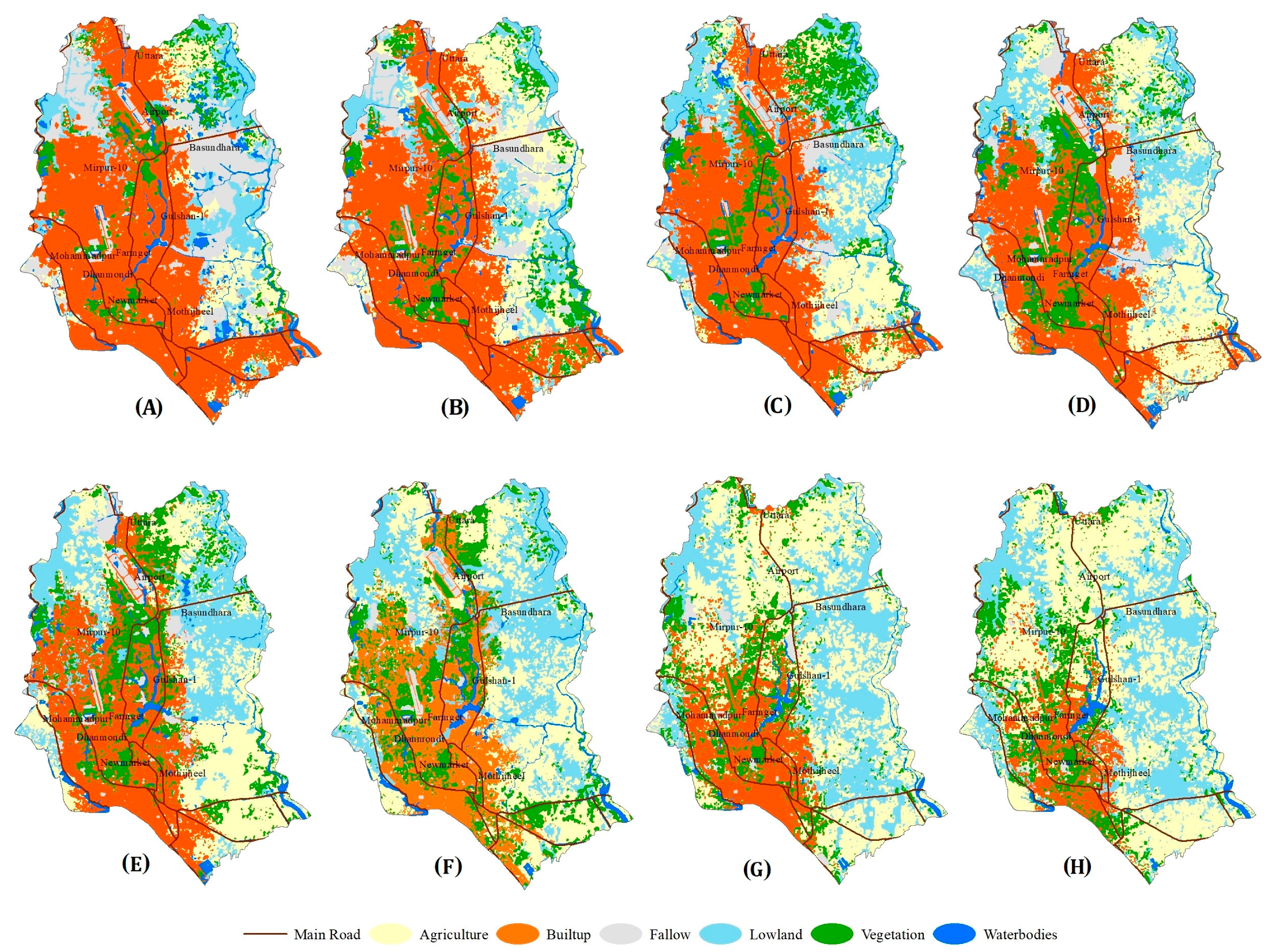
The spatial pattern of urban expansion between 1972 and 2015 suggests that Dhaka and its neighboring areas have witnessed notable urban expansion in the peri-urban and suburban areas, accompanied by a significant recent increase in population growth. Figure 3 presents the land use and land cover maps of greater Dhaka for the eight time periods (e.g., 1972, 1980, 1990, 1995, 2000, 2005, 2010, and 2015). Each growth center in the following discussion is presented separately to identify areas with significant land cover transformation and facilitate a more detailed understanding of urban pattern and trajectories across the region.
Through a comparison of the land cover maps generated in this study, along with close investigation of historical topographic maps and the empirical literature, it has been observed that there are three primary growth centers in the study area, specifically Savar in the northwest, Naryangang in the east, and Dhaka in the center, located on the banks of the rivers Dhaleswari, Lakkhya, and Buriganga, respectively [23,56]. These three mighty rivers fed the initial growth of these cities as they provided year-round navigable channels for trade, transportation, and commerce for the entire region. The area where the primary township developed was at a comparatively higher elevation than the surroundings (see Figure 1), and was thus safe from erosion and flooding and easily serviced by a water linkage.
Dhaka’s urban growth gained momentum only after 1950 when a large influx of Muslim migrants from India [22,57] resulted in rapid population growth in the city territory, from 335,935 in 1951 to 556,712 in 1961, with a net growth rate of 65% [58]. Such a huge and unexpected population explosion created enormous pressure on Dhaka’s existing housing and urban infrastructure and thus demanded land for further development that is away from the old city but readily available for housing and infrastructure development. As a result, major urban development projects during that time were initiated in the immediate north of the old city such as in Banani, Gulshan, and Baridhara, with 140 hectares, 290 hectares, and 150 hectares, respectively, acquired for high-class residential developments [23]. In addition, another 500 acres of agricultural land was acquired in the northwest in Dhanmondi for high-class residential development, following the recommendation of a sub-committee created by the East Pakistan planning division in 1948. Although this residential plan was only partially executed, the impacts of these housing developments have been quite significant in terms of the physical structure and spatial dimension of the city. Since then the city has expanded northward and high-class residential areas are constantly attempting to keep themselves at the northern periphery of the city (Figure 3).
The actual urban development in Dhaka, however, has increased drastically since 1971, when Dhaka became the national capital of the new sovereign state of Bangladesh. Even in the 1960s Dhaka was experiencing a very rapid population growth of over 6% annually, and this growth became much faster after 1971, with the population reaching 1,772,000 in 1974 from only 557,000 in 1961 [58]. The thematic map of 1972 representing built-up areas during that time in Dhaka was approximately 2750 ha or 9% of the total DCC areas (Table 4). Its immediate neighboring cities such as Gazipur, Naryanganj, and Savar were small townships with estimated built-up areas of approximately 243 ha, 238 ha, and 30 ha, respectively. Agricultural land (60%), lowland (21%), and vegetation cover (13%) were the dominant land cover types in 1972, and accounted for 96% of the study area. While in the DCC area those land cover classes were still higher contributors, their amounts were lowered to 47% for agricultural, 28% for lowland, and 14% for vegetation cover (Figure 4).
Major built-up area in the DCC area in the early 1970s still occupied the core city, but also expanded beyond the old city limits. In the period between 1972 and 1980, the built-up area in the DCC area clearly headed towards the west and north of the existing growth center (Figure 3 and Figure 5). The total built-up area had by this time increased by 72%, while the population in the DCC areas increased to 3,248,000, with a net growth rate of 120% [59,60]. Later population growth slowed down, but it was still at a startling rate in the following period. For example, between 1980 and 1990, Dhaka’s population doubled in size from 3,248,000 in 1980 to 6,619,000 in 1990, with an estimated population growth rate of 104% [61] and built-up growth rate of 46% during the same period.
By this time, Dhaka experienced dense development and clear expansion towards the north, northeast, and northwest by engulfing remnants of open and undeveloped land in core city areas (Figure 5). Developed land, as seen in this period (1980–1990), clearly expanded to Adabar, Mirpur-1, Mirpur-11 and Airport in the north and further north to the banks of the Turag River. A visible amount of developed land, as seen in 1990 maps of Tongi bazar (Gazipur) and the surrounding industrial areas, were the main impetus for urban development (Figure 3). The expansion of the city to the east and west was limited due to the presence of a huge depression between Dhaka and Savar, which resulted in major development having to occur in other directions, such as the rapid expansion along the north–south corridor of Dhaka City. While beyond the city limits to the north and northwest crosses into depression areas, vast lands were rural and agriculture in use, actively working as hinterland for Dhaka and yet to be incorporated within the full continuum of urban development by 1990.
Although built-up areas were small patches of the whole study area during the early period of this study, they rapidly increased in size in the following years, due in part to the booming business of export-oriented garment industries in Bangladesh. This type of business expansion had enormous impacts on urban growth in and around Dhaka as it contributed to industrialization and job opportunities in the cities, and spurred the mass movement of the surplus population away from the countryside [23]. As elevated land in the city has already been urbanized during the rapid urban development since the 1980s, such industrial expansion coupled with residential development could only expand to the north (Tongi-Gazipur) or by reclaiming the vast depression land in the east and west of the core city. As a result, arable and wetland areas, mainly located adjacent to the existing urban edge, have become the target of urban expansion, particularly since the 1990s. As such, land filling was triggered in the outskirts of the capital, engulfing canals, paddy fields, waterways, and the vast depression areas in the east and west of the city. As observed from land cover maps of 1990, major landfilling areas are identified in several locations such as in Khilkhet (Bashundhara Residential Area) and Mirpur (Duaripara and Rupganj). As a result, landfill area increased its proportional share from 475 hectares in 1980 to 801 hectares in 1990 in the DCC area (Table 4). As population pressure with industrial development continued to increase in the city limits, landfilling battles on the city outskirts concurrently increased at a rapid rate in the following decades. For example, fallow land reached 2144 hectares in 2000 and 4067 hectares in 2015 with a net growth rate of 45% and 127%, respectively (Table 4). The major landfilling areas are still identified in the eastern part of the city, such as Khilkhet in the Bashundahra Residential Area and other new locations at Aftabnagar, Banasree, and Karial (Figure 5). Between 2000 and 2015, the study area observed landfills in all directions including the existing location, and continuous expansion of the area that had been previously filled up. However, this time landfilling extended to the southeast along the Dhaka–Naryanganj highway and to the east in Keraniganj, crossing the river of Buriganga.
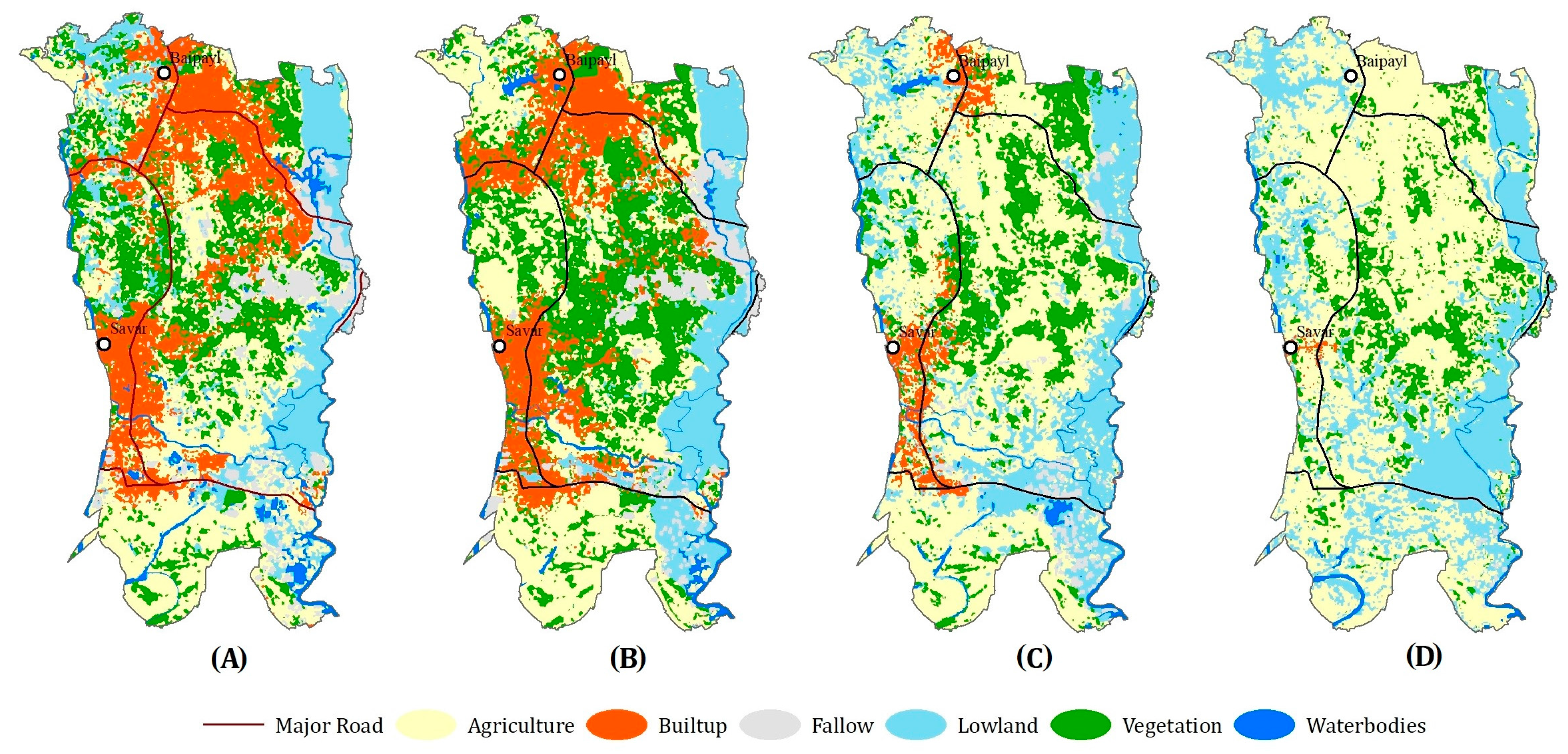
The initial urban development in Savar was on the northeast bank of the Dhaleswari River and the small township was located between the present Namabazar and Savar Thana (Figure 6). The whole region to the north, east, and south was largely agricultural or marshy land. As estimated from the thematic map of 1972, approximately 14,580 hectares or 58% was agricultural and 6954 hectares or 27% of the total land area in Savar was lowland (Table 5). An analysis of the land cover map of the Savar area reveals that the built-up area had increased between 1972 and 1980 by approximately 211%, while the population growth was around 92% (estimated from the 1974 to 1981 census) [59].
The trend of urban growth in Savar continued in the following years, but the rate was substantially higher than in the past. For example, in the period between 1990 and 1995 the total urban growth in Saver was approximately 325%, with an annual increase rate of 34%. Later developed land doubled in size as it increased from 628 hectares in 1995 to 1274 hectares in 2000, with a net increase rate of 103%. Although developed land continued to increase, the rate of growth was higher in the period of 2005–2010; the total built-up area reached 4660 hectares in 2010, with a net growth rate of approximately 150%. Population growth in the same period was highest at around 130% between the 2001 and 2011 census periods [62,63].
In 1974 Savar was a city with 131,429 inhabitants [58], but urban development pressure in Savar resulted from the establishment of a number of planned large-scale industrial zones, such as the Dhaka Export Processing Zone in Dhamsona in the early 1990s and heavy industrial plants in Nayarhat in the mid-1970s. As a result, the population swelled, due mainly to a great influx of rural migrants looking for work in the booming industrial sectors in Savar [23,57]. In addition, a number of establishments with growing tourism importance such as Jahanginrangar University, the Savar Cantonment, the Atomic Energy Center, and the National Memorial, have further reinforced development of Savar.
The southeastern city of Naryanganj was mainly known in the past as a salt trading center and for having the largest jute mill, high numbers of cotton mills, and other large-scale industrial plants. In its initial period, urban development was limited to the eastern and western banks of the Lakkhya river, as seen in the land cover map of 1972 (Figure 7): approximately 238 hectares of land were covered with built-up area (Table 6). The outer peripheral expansion of this city in the south was up to the Kashipur River and towards the north up to the Adamjee EPZ. Later, expansion of huge cotton industries in the early 1990sn along with other large-scale industrial development, meant the city underwent rapid urbanization to accommodate the growing number of workers and associated infrastructure development. As a result, between 1980 and 1990 the built-up area increased to 83%. This time the city is expanding towards the northwest, following the old axis of the Dhaka–Naryanganj highway, but, due to physical constraints such as the river Buriganga to the south and the flood-prone swampy land to the north, urban development away from the road was slow.
Nevertheless, due to the aftermath of the 1988 floods, this swampy land in the northwest outskirts of Naryanganj city and southeast periphery of Dhaka City, literally called Dhaka Naryanganj Demra (DND) flood protection dam, originally meant to protect the land from flooding and improve agricultural production, became the main target of residential development [64]. As a result, a large area in the DND area experienced rapid and chaotic urban development, which resulted in rapid land conversion from agricultural–lowland to residential development (Figure 7). Built-up area, therefore, increased from 612 hectares in 1990 to 1720 hectares in 2000, a net growth rate of 181%. The developed land in Narayanganj is expanding much faster in recent times due to the establishment of several planned industrial estates in Enayetnagar, Fatullaha, Adamje, Kachpur, and Panchabati, which has made the city one of the largest urban agglomerations in the region.
Beyond the Buriganga River, Keraniganj was primarily rural and dominated by various agricultural types. The built-up area estimated from the land cover map of 1972 (Figure 3) was approximately 138 hectares, while agricultural was around 12,305 hectares or 70% of the total land in Keraniganj. However, these areas have undergone rapid urbanization in recent times due to several connecting bridges over Buriganga, which established a quick gateway to Dhaka and the rest of the south Keraniganj. The major urban development in Keraniganj is now found in the immediate south bank of Buriganga, in such locations as Zinzira, Ragunathpur, Mandail, Kalindi, Barisur, Dakpara, Kaliganj, and up towards Mirerbag. In addition, the area also houses a number of small- and medium-scale manufacturing industries, warehouses, and lower-income residences. These manufacturing industries, along with ongoing massive-scale residential development projects in Ekuria, are making this area urbanize rapidly in recent times. As shown in the land cover map for 1990 to 2015 (Figure 3), the total built-up area in Keraniganj increased by 764%, while fallow land increased by 1052% (Table 7).
The area statistics derived from the land cover maps reveal that urban growth in the northern outskirts of Dhaka city in Gazipur (Figure 8) increased significantly, from 243 hectares in 1972 to 7640 hectares in 2015, with a total growth rate of 3038% (Table 7). This built-up growth rate is substantially higher than any other urban center studied here. Among the eight time periods, the highest urban growth in the region was recorded in the 1972–1980 and 2005–2010 periods at the rate of 145% and 100%, respectively. This growth can be attributed to both industrial development and expansion and human population growth in the region. Specifically, this area contains five universities, a high-tech park, a number of government, semi-government, and private offices, and the largest concentration of garment manufacturing industries in the countree. Due to the availability of flood-free, low-cost land with close proximity to the core city area, Gazipur has become the main target of both residential and industrial development in recent times. As a result, arable agricultural land and lowland cover types have been converted to developed land very quickly. As observed in the 43-year period, the total agricultural land dropped to 6784 hectares by 2015 from 25,186 hectares in 1972, a 73% decrease. The land cover statistics also suggest that vegetation cover in the region has increased over the 43-year study period; however, except for the forest cover in the north, this increase in vegetation is actually an increase in peri-urban settlement. These settlements are covered with homestead vegetation, as is typical across Bangladesh.
In the smallest administrative unit, Bandar, which is located on the eastern bank of the Shitallakhya River, the dominant land cover change is an increase in developed land (Figure 3). While the dominant land use is agriculture (41%), the land cover maps for the last 43 years show that developed land increased from 98 hectares in 1972 to 1532 hectares in 2015, with a net growth rate of 910%. The greatest increase is observed between 1995 and 2000, when the total built-up growth was 137% (Table 7). Within this conversion to developed land, the largest portion is industrial and port-related infrastructure development, which has expanded along the eastern bank of the Shitallakhya River in a north–south direction. This built-up expansion was mainly at the expense of agricultural land as the total area of agricultural land declined at a rate of approximately 34%, from 3549 hectares to 2362 hectares, across the period. The landfill area during the same period also increased substantially, from only 2 hectares in 1972 to 175 hectares in 2015. Much of these landfills are comprised of brickfields, which are expanding east and south out from the center.
Among the other three connecting growth centers (i.e., Soanrgaon, Rupganj, and Kaliganj) in this study, increasing cover of developed land was documented in Soanargaon and Rupganj, both of which are located in the southeast and east of the study area (Figure 1 and Figure 3). The development of Sonargaon was historically significant as it was the capital of Bangladesh in the 15th century. The urban development of this historic city gained momentum in recent times due to the significant increase of tourism-related services, educational institutions, and various private residential development projects. As such, developed land in Sonargaon has increased rapidly between 2000 and 2015, from 185 hectares to 851 hectares, with a net growth rate of 360%. Similarly, in Rupganj, urban area markedly increased from 197 hectares in 2000 to 1287 hectares in 2015, a net growth rate of 553% (Table 7). Additionally, the landfill area in Rupganj has increased since 1990, with 738 hectares in 2000 from only 30 hectares in 1990. This growth remained constant in the following year but at an accelerated rate, i.e., it reached 1840 hectares in 2010 and 3082 hectares in 2015 with total growth at a rate of 149% and 67%, respectively. Kaliganj in the northeast of this study area is a predominantly agricultural, rural, and peri-urban settlement (53% in total). The land use survey of 2006 estimates that 23% of the total land of Tongi, Gazipur, Kaliganj, and Rupganj was residential, including urban housing, rural homesteads, and informal housing; less than 1% is designated for industrial and commercial uses and 60% land is used for agricultural purposes [65].The recent land use survey conducted by RDP, RAJUK 2013 [66] estimated that residential land use comprises 36.5% of the current study area, while industrial and commercial uses comprise 2.6% and 1%, respectively. The total built-up area including residential, industrial, public facilities, road networks, commercial, and mixed use comprises 44% of the survey area, which closely aligns with our findings of 45% including urban and rural settlements (except for the small patches of forest in the north, vegetation classes in our study correspond with rural settlements, which account for almost 20%).
3.3. Urban Growth Trajectory Analysis
The spatial pattern of urban expansion between 1972 and 2015 suggests that Dhaka and its surrounding areas have experienced rapid urbanization, which has resulted in significant changes in land use over the 43-year period studied here. The spatial trajectory of urban expansion over the study period suggests that north, northwest, and southeast were the major directions experiencing urban development (Figure 9). By contrast, southern and western expansion are relatively low since the southern and western zones are dominated by low-lying marshy land, which clearly constrained the growth of built-up areas in these directions. The urban growth was estimated from the thematic map over the 43-year period in the direction toward the north (35% expansion), along the Dhaka–Mymensingh highway (Tongi-Gazipur) and northwest (30% expansion), the Savar–Ashulia corridor along the Dhaka–Aricha highway, and also toward the southwest (25.6%) along the Dhaka–Narayanganj and Dhaka–Chittagong highways (Figure 9). The development towards the north was significant due to comparatively flood-free land in that direction and particularly a number of development projects, such as shifting the airport from its old site at Tejgaon to its new site north of Kurmitola, which is about 10 km north of the old airport.
Another major development project is the Uttara Model Town located immediately north of the new airport. North of Uttara stands the industrial town of Tongi and beyond Tongi and Joydebpur has also been partly filled up with the establishment of two institutions of higher learning, the National University, and the Islamic University of Technology. Due to population growth and the subsequent expansion of trade and commerce, the current development of the city is radiating southwest, north, northeast, west, and northwest from the banks of the Burignaga River and extending into rural areas and beyond the outskirts. Dhaka’s recent growth has been linked with Narayanganj and Gazipur City, such that there are no gaps between Dhaka and those two connecting cities.
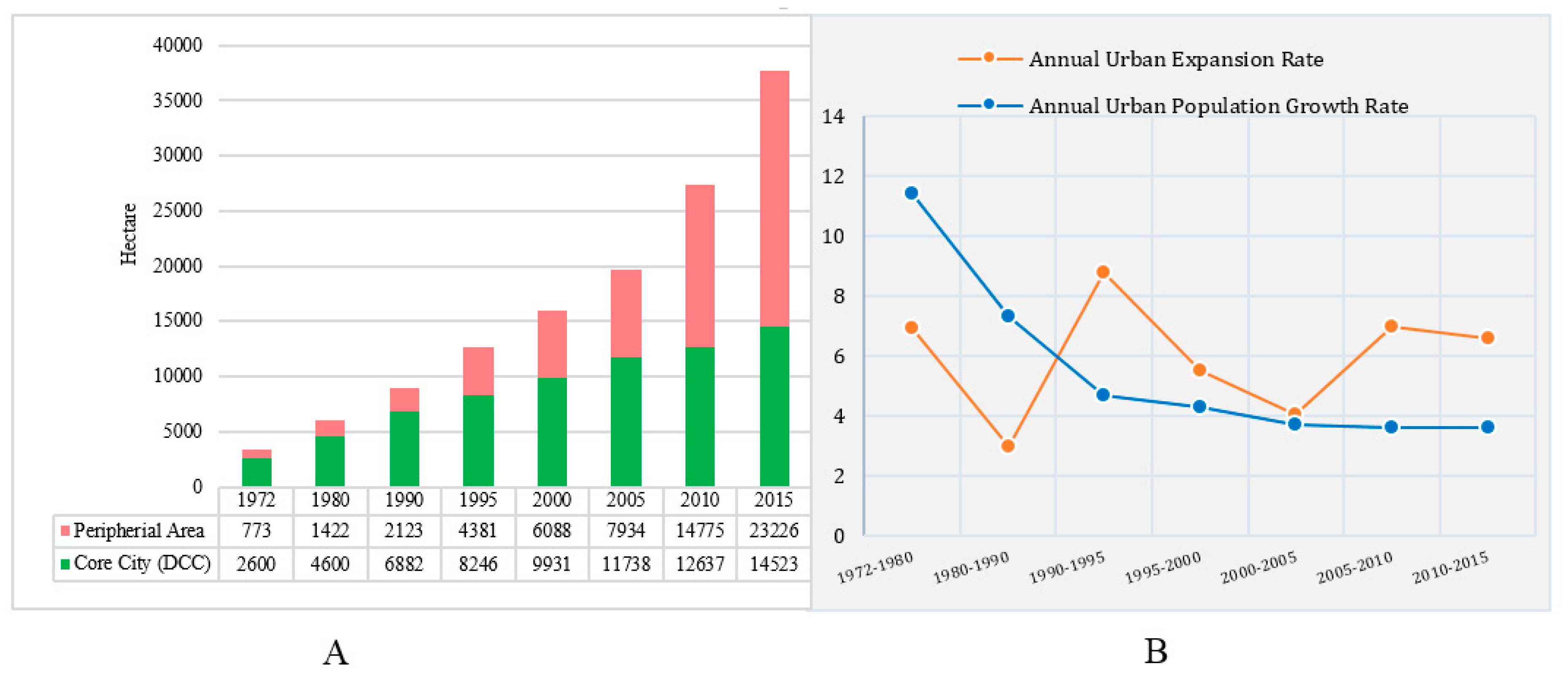
The spatial information derived from the time-series analysis land cover maps over the 43-year period shows that a continuous increase in built-up land occurred, at a rate much faster than the urban population growth in all connecting cities in this study. For example, between 1972 and 1980 and 1980 and 1990, the annual population growth rate was higher at 11.4% and 7.3%, respectively, while the urban expansion rate was only 7% and 3%, respectively (Figure 10B). Later population growth continued to fluctuate around 3.5% per annum, but the urban expansion rate maintained stable growth trends at around 6% until the end of the study period. Another important feature of this urban growth, as presented in Figure 10, is that peripheral growth was higher throughout the study period than the core city area (Figure 10A). In the 43-year period the total peripheral growth rate was 2903%, while that of the core city area was 459%.
In this study we utilized eight dates of imagery to develop our time series with different sensors and spatial resolutions. Since these images were not captured at the same time, the water level in permanent reservoirs such as ponds, rivers, canals, and seasonal wetlands was variable. As can be seen, actual quantities of water bodies and wetlands do fluctuate in different periods; however, the general trend is that wetlands in peri-urban areas were encroached on heavily by agricultural pressure, brickfield expansion, or landfilling. The areas where these processes were taking place are identified in the land cover maps. A possible explanation for this rampant urban development and encroachment in the city outskirts is the lack of space in the core area for further development, combined with the somewhat inadequate public policies concerning these wetlands and their environmental protection.
The Greater Dhaka Area is a bustling megacity with more than 18 million people, making it one of the most populated cities in the world, with a density of 23,234 inhabitants per square kilometer within the core city area (DCC). Like other megacities in the developing world, such huge population growth in association with inadequate urban services and lack of authorities’ reign over growth management has led to an increase in environmental degradation, exponentially growing slums, and increases in pollution, poverty, disease, crime, land grabbing, corruption, and traffic congestion. Fifty-five government agencies work to provide civic services in Dhaka, all typically following their own trajectories in decision-making, which often leads to chaos among the differing authorities, rarely reflecting citizens’ wishes in the implementation of development plans. In terms of driving urban expansion, existing planning guides played little role compared to individual and corporate agents such as real-estate developers, industrial entrepreneurs, investors, and other vested groups. Real-estate developers and manufacturing investors, such as export-oriented garment manufacturers in the city outskirts, have been instrumental in shaping urban development in Dhaka. Hence, this study’s findings highlight that a rapidly growing city like Dhaka should be managed through the proactive protection of natural and ecologically sensitive areas, along with the involvement of landowners, locals, land developers, and multilevel stakeholders based on a shared long-term vision concerning the most desirable and sustainable urban growth for Bangladesh.
4. Conclusions
Using multi-sensor time series satellite data and an ensemble classifier “Random Forest” with socioeconomic, demographic, and biophysical information, this study quantifies spatiotemporal land cover change and captures the full continuum of urban expansion in the megacity of Dhaka, Bangladesh, over a 43-year period. Employing Random Forest, the new classification algorithm in this study has shown high classification accuracy (e.g., overall accuracies of 85–97%) with the ability to discriminate minute details of land cover classification in the complex and heterogeneous landscape represented by such complex, urban land cover. Among the six land cover types, the agricultural class was the dominant land cover type throughout the study period. Its total volume, however, has declined significantly from 921 km2 in 1972 to 414 km2 in 2015, with a net decline of 55% over the 43-year study period. This rate was higher in the DCC with 142 km2, which accounted for 47% of the DCC area in 1972, and dropped to 33 km2, covering only 10% of DCC areas in 2015—a net decline of 77%. Compared to Dhaka City, neighboring cities like Gazipur in the north and Savar in the west experienced higher urban development during that period. The total urban development between 1972 and 1980 in Gazipur was 145% and in Savar was 211%, with annual growth rates of about 12% and 15%, respectively. This rapid urban growth with indiscriminate land reclamation processes has resulted in the degradation of agricultural land, forests, vegetated areas, wetlands, and water bodies across the whole region. The built-up area and fallow land in the same period in DCC increased by 459% and 3561%, respectively, while in the study region the net growth rates of built-up land and fallow land were substantially higher at 1019% and 11,270%, respectively. Major expansion occurred to the north, northwest, and southwest, consuming agricultural land, vegetation cover, and bodies of water. This increase in urban development resulted in a loss of agricultural land, vegetation cover, and bodies of water. In addition, the findings highlight the increasing vulnerability of ecologically sensitive wetlands in urban and peri-urban areas, which have largely been degraded and encroached on by the expansion of brickfield and landfilling. This study has highlighted that time series analysis of remotely sensed data and non-parametric, regression-based machine learning algorithms can be utilized to accurately classify complex, heterogeneous urban land cover with quite high classification accuracy. The methods and techniques employed in this study may serve as guidelines for future applications across varied landscapes. Furthermore, the resulting land cover maps and spatial information generated from this study may assist planners, stakeholders, and academia with gaining a detailed understanding of land cover change, urban growth patterns, and associated ecological risk in Dhaka’s mega-urban region of Bangladesh, thus helping to make better planning decisions for a more sustainable urban future.
Acknowledgments
The authors are grateful to the assistant editor and two unnamed reviewers for their constructive comments and suggestions that helped us to improve the manuscript. We also thankful to Amran Hossan (Cartography Lab), Masudur Rahman (Disaster Research, Training and Management Centre) and Urban Studio, Department of Geography and Environment, University of Dhaka for providing GIS data. Mohammad Mehedy Hassan is especially thankful to UF Geography for providing Graduate Student Fellowship (GSF).
Author Contributions
In this article, Mohammad Mehedy Hassan was responsible for research design, running the Random Forest analysis, and writing the paper. Jane Southworth was responsible for the research guiding and editing.
Conflicts of Interest
The authors declare no conflict of interest.
References
- United Nations. World Urbanization Prospects, 2014 Revision (United Nations, New York). Available online: https://esa.un.org/unpd/wup/Publications/Files/WUP2014-Report.pdf (accessed on 20 September 2017).
- UN-Habitat. Urbanization and Development—Emerging Futures. World Cities Report 2016; UN-Habitat: Nairobi, Kenya, 2016; Available online: http://wcr.unhabitat.org/wp-content/uploads/2017/02/WCR-2016-Full-Report.pdf (accessed on 20 September 2017).
- United Nations. The World’s Cities in 2016: Data Booklet. Econ. Soc. Aff. 2016, 29. Available online: http://www.un.org/en/development/desa/population/publications/pdf/urbanization/the_worlds_cities_in_2016_data_booklet.pdf (accessed on 20 September 2017).
- Demographia. Demographia World Urban Areas, 13th Annual Edition: 2017:04. Available online: http://www.demographia.com/db-worldua.pdf (accessed on 20 September 2017).
- World Bank. Bangladesh-Towards Accelerated, Inclusive and Sustainable Growth: Opportunities and Challenges: Overview; World Bank: Washington, DC, USA, 2012; Volume II, Main Report; Available online: http://documents.worldbank.org/curated/en/132321468014348379/Overview (accessed on 22 September 2017).
- Ahmed, F.; Bibi, M.H.; Monsur, M.H.; Ishiga, H. Present environment and historic changes from the record of lake sediments, Dhaka City, Bangladesh. Environ. Geol. 2005, 48, 25–36. [Google Scholar] [CrossRef]
- Economist Intelligence Unit (EIU). The Global Liveability Report 2017: A Free Overview; EIU: London, UK, 2017; Volume 14, Available online: http://pages.eiu.com/rs/753-RIQ-438/images/Liveability_Free_Summary_2017.pdf (accessed on 22 September 2017).
- Yao, X.; Wang, Z.; Wang, H. Impact of Urbanization and Land-Use Change on Surface Climate in Middle and Lower Reaches of the Yangtze River, 1988–2008. Adv. Meteorol. 2015. [Google Scholar] [CrossRef]
- Serneels, S.; Linderman, M.; Lambin, E.F. A multilevel analysis of the impact of land use on interannual land-cover change in East Africa. Ecosystems 2007, 10, 402–418. [Google Scholar] [CrossRef]
- Su, S.; Xiao, R.; Jiang, Z.; Zhang, Y. Characterizing landscape pattern and ecosystem service value changes for urbanization impacts at an eco-regional scale. Appl. Geogr. 2012, 34, 295–305. [Google Scholar] [CrossRef]
- Lambin, E.F.; Meyfroidt, P. Global land use change, economic globalization, and the looming land scarcity. Proc. Natl. Acad. Sci. USA 2011, 108, 3465–3472. [Google Scholar] [CrossRef] [PubMed]
- Foley, J.A.; Defries, R.; Asner, G.P.; Barford, C.; Bonan, G.; Carpenter, S.R.; Chapin, F.S.; Coe, M.T.; Daily, G.C.; Gibbs, H.K.; et al. Global consequences of land use. Science 2005, 309, 570–574. [Google Scholar] [CrossRef] [PubMed]
- Brown, S.; Versace, V.L.; Laurenson, L.; Ierodiaconou, D.; Fawcett, J.; Salzman, S. Assessment of spatiotemporal varying relationships between rainfall, land cover and surface water area using geographically weighted regression. Environ. Model. Assess. 2012, 17, 241–254. [Google Scholar] [CrossRef]
- Asgarian, A.; Amiri, B.J.; Sakieh, Y. Assessing the effect of green cover spatial patterns on urban land surface temperature using landscape metrics approach. Urban Ecosyst. 2015. [Google Scholar] [CrossRef]
- Su, S.; Ma, X.; Xiao, R. Agricultural landscape pattern changes in response to urbanization at ecoregional scale. Ecol. Indic. 2014, 40, 10–18. [Google Scholar] [CrossRef]
- Southworth, J.; Munroe, D.; Nagendra, H. Land cover change and landscape fragmentation—Comparing the utility of continuous and discrete analyses for a western Honduras region. Agric. Ecosyst. Environ. 2004, 101, 185–205. [Google Scholar] [CrossRef]
- Rahman, H.Z. Urbanization in Bangladesh: Challenges and Priorities. Bangladesh Econ. Forum. 2014, 21–22. Available online: http://www.pri-bd.org/upload/file/bef_paper/1414213688.pdf (accessed on 2 October 2017).
- Dewan, A.M.; Yamaguchi, Y. Using remote sensing and GIS to detect and monitor land use and land cover change in Dhaka Metropolitan of Bangladesh during 1960–2005. Environ. Monit. Assess. 2009, 150, 237–249. [Google Scholar] [CrossRef] [PubMed]
- Ahmed, S.; Bramley, G. How will Dhaka grow spatially in future? Modelling its urban growth with a near-future planning scenario perspective. Int. J. Sustain. Built. Environ. 2015, 4, 359–377. [Google Scholar] [CrossRef]
- Zhang, Q.; Seto, K.C. Mapping urbanization dynamics at regional and global scales using multi-temporal DMSP/OLS nighttime light data. Remote Sens. Environ. 2011, 115, 2320–2329. [Google Scholar] [CrossRef]
- Ahmed, S.U. Dacca—A Study in Urban History and Development; Curzon Press: London, UK, 1986. [Google Scholar]
- Rabbani, G. Dhaka: From Mughal Outpost to Metropolis; University Press Limited: Dhaka, Bangladesh, 1997. [Google Scholar]
- Islam, N. Dhaka from City to Megacity: Perspectives on People, Places, Planning and Development Issues; Urban Studies Program, Department of Geography, University of Dhaka: Dhaka, Bangladesh, 1996. [Google Scholar]
- Kabir, A.; Parolin, B. Planning and development of Dhaka—A story of 400 years. In Proceedings of the 15th International Planning History Society Conference, Cities, Nations and Regions in Planning History, Sao Paulo, Brazil, 15–18 July 2012; Volume 1, pp. 1–20. [Google Scholar]
- Ahammed, F.; Hewa, G.A.; Argue, J.R. Variability of annual daily maximum rainfall of Dhaka, Bangladesh. Atmos. Res. 2014, 137, 176–182. [Google Scholar] [CrossRef]
- Li, Q.; Lu, L.; Weng, Q.; Xie, Y.; Guo, H. Monitoring urban dynamics in the Southeast, U.S.A. using time-series DMSP/OLS nightlight imagery. Remote Sens. 2016, 8, 578. [Google Scholar] [CrossRef]
- Hassan, M.M.; Nazem, M.N.I. Examination of land use/land cover changes, urban growth dynamics, and environmental sustainability in Chittagong city, Bangladesh. Environ. Dev. Sustain. 2016, 18. [Google Scholar] [CrossRef]
- Hassan, M.M. Monitoring land use/land cover change, urban growth dynamics and landscape pattern analysis in five fastest urbanized cities in Bangladesh. Remote Sens. Appl. Soc. Environ. 2017, 7, 69–83. [Google Scholar] [CrossRef]
- Yu, W.; Zhou, W.; Qian, Y.; Yan, J. A new approach for land cover classification and change analysis: Integrating backdating and an object-based method. Remote Sens. Environ. 2016, 177, 37–47. [Google Scholar] [CrossRef]
- Dou, Y.; Liu, Z.; He, C.; Yue, H. Urban land extraction using VIIRS nighttime light data: An evaluation of three popular methods. Remote Sens. 2017, 9, 175. [Google Scholar] [CrossRef]
- Yuan, F.; Sawaya, K.E.; Loeffelholz, B.C.; Bauer, M.E. Land cover classification and change analysis of the twin cities (Minnesota) metropolitan area by multitemporal landsat remote sensing. Remote Sens. Environ. 2005, 98, 317–328. [Google Scholar] [CrossRef]
- Rutherford, G.N.; Bebi, P.; Edwards, P.J.; Zimmermann, N.E. Assessing land-use statistics to model land cover change in a mountainous landscape in the European Alps. Ecol. Model. 2008, 212, 460–471. [Google Scholar] [CrossRef]
- Weng, Q. Remote sensing of impervious surfaces in the urban areas: Requirements, methods, and trends. Remote Sens. Environ. 2012, 117, 34–49. [Google Scholar] [CrossRef]
- Deilmai, B.R.; Ahmad, B.B.; Zabihi, H. Comparison of two classification methods (MLC and SVM) to extract land use and land cover in Johor Malaysia. IOP Conf. Ser. Earth Environ. Sci. 2014, 20, 12052. [Google Scholar] [CrossRef]
- Xu, X.; Min, X. Quantifying spatiotemporal patterns of urban expansion in China using remote sensing data. Cities 2013, 35, 104–113. [Google Scholar] [CrossRef]
- Akar, Ö.; Güngör, O. Classification of multispectral images using Random Forest algorithm. J. Geod. Geoinf. 2012, 1, 105–112. [Google Scholar] [CrossRef]
- Breiman, L. Random Forests. Mach. Learn. 2001, 45, 5–32. [Google Scholar] [CrossRef]
- Belgiu, M.; Dragut, L. Random Forest in remote sensing: A review of applications and future directions. ISPRS J. Photogramm. Remote Sens. 2016, 114, 24–31. [Google Scholar] [CrossRef]
- Mountrakis, G.; Im, J.; Ogole, C. Support vector machines in remote sensing: A review. ISPRS J. Photogramm. Remote Sens. 2011, 66, 247–259. [Google Scholar] [CrossRef]
- Qian, Y.; Zhou, W.; Yan, J.; Li, W.; Han, L. Comparing machine learning classifiers for object-based land cover classification using very high resolution imagery. Remote Sens. 2015, 7, 153. [Google Scholar] [CrossRef]
- Anderson, J.R.; Hardy, E.E.; Roach, J.T.; Witmer, R.E. A Land Use/Land Covers Classification System for Use with Remote Sensor Data. U.S. Geological Survey Professional Paper. USGS 1976, 964, 1–26. [Google Scholar]
- Hastie, T.; Tibshirani, R.; Friedman, J. The Elements of Statistical Learning: Data Mining, Interface and Prediction; Springer: New York, NY, USA, 2009. [Google Scholar]
- Zhang, H.S.; Zhang, Y.Z.; Lin, H. Urban land cover mapping using Random Forest combined with optical and SAR data. In Proceedings of the IEEE International Geoscience and Remote Sensing Symposium (IGARSS), Munich, Germany, 22–27 July 2012; pp. 6809–6812. [Google Scholar]
- Pierce, A.D.; Farris, C.A.; Taylor, A.H. Forest ecology and management use of Random Forests for modeling and mapping forest canopy fuels for fire behavior analysis in Lassen Volcanic National Park, California, USA. For. Ecol. Manag. 2012, 279, 77–89. [Google Scholar] [CrossRef]
- Hapfelmeier, A.; Ulm, K. Variable selection by Random Forests using data with. Comput. Stat. Data Anal. 2014, 80, 129–139. [Google Scholar] [CrossRef] [Green Version]
- Archer, K.J.; Kimes, R.V. Empirical characterization of Random Forest variable importance measures. Comput. Stat. Data Anal. 2008, 52, 2249–2260. [Google Scholar] [CrossRef]
- Horning, N. Random Forests: An algorithm for image classification and generation of continuous fields data sets. Remote Sens. Environ. 2010, 199, 154–166. [Google Scholar]
- Chrysa, I.; Mallinis, G.; Gitas, I.; Tsakiri-strati, M. Remote sensing of environment estimating Mediterranean forest parameters using multi seasonal Landsat 8 OLI imagery and an ensemble learning method. Remote Sens. Environ. 2017, 199, 154–166. [Google Scholar] [CrossRef]
- Oliveira, S.; Oehler, F.; San-miguel-ayanz, J.; Camia, A.; Pereira, J.M.C. Forest ecology and management modeling spatial patterns of fire occurrence in Mediterranean Europe using multiple regression and Random Forest. For. Ecol. Manag. 2012, 275, 117–129. [Google Scholar] [CrossRef]
- Rodriguez-galiano, V.F.; Chica-olmo, M.; Abarca-hernandez, F.; Atkinson, P.M.; Jeganathan, C. Remote sensing of environment Random Forest classification of mediterranean land cover using multi-seasonal imagery and multi-seasonal texture. Remote Sens. Environ. 2012, 121, 93–107. [Google Scholar] [CrossRef]
- Jensen, J.R. Introductory Digital Image Processing, 3rd ed.; Prentice Hall: Upper Saddle River, NJ, USA, 2005. [Google Scholar]
- Ghosh, A.; Sharma, R.; Joshi, P.K. Random Forest classification of urban landscape using landsat archive and ancillary data : Combining seasonal maps with decision level fusion. Appl. Geogr. 2014, 48, 31–41. [Google Scholar] [CrossRef]
- Janitza, S.; Tutz, G.; Boulesteix, A. Random Forest for ordinal responses: Prediction and variable selection. Comput. Stat. Data Anal. 2016, 96, 57–73. [Google Scholar] [CrossRef]
- Eisavi, V.; Homayouni, S. Land cover mapping based on Random Forest classification of multitemporal spectral and thermal images. Environ. Monit. Assess. 2015, 187. [Google Scholar] [CrossRef] [PubMed]
- Congalton, R.G.; Green, K. Assessing the Accuracy of Remotely Sensed Data: Principles and Practices; CRC Press Taylor & Francis Group: London, UK, 2009. [Google Scholar]
- Rahman, M.; Zaman, K.B.; Hafiz, R. Translating text into space for mapping the past territory of a city: A study on spatial development of Dhaka during Mughal period. City Territ. Archit. 2016, 3, 7. [Google Scholar] [CrossRef]
- Amin, A. Dhaka’s Informal Sector and its Role in the Transformation of Bangladesh Economy; Ahmed, S.U., Ed.; Dhaka Past Present Future; The Asiatic Society: Dhaka, Bangladesh, 1991; pp. 446–470. [Google Scholar]
- Bangladesh Bureau of Statistics (BBS). Bangladesh Population Census; Dacca District; Government of Bangladesh: Dhaka, Bangladesh, 1974.
- Bangladesh Bureau of Statistics (BBS). Bangladesh Population Census 1981; Government of Bangladesh: Dhaka, Bangladesh, 1983.
- Bangladesh Bureau of Statistics (BBS). Bangladesh Population Census 1981; Dhaka Statistical Metropolitan Area (Dhaka, S.M.A.), Ministry of Planning, Government of Bangladesh: Dhaka, Bangladesh, 1985.
- Bangladesh Bureau of Statistics (BBS). Bangladesh Population Census 1991; Ministry of Planning, Government of Bangladesh: Dhaka, Bangladesh, 1993.
- Bangladesh Bureau of Statistics (BBS). Bangladesh Population and Housing Census 2001; Urban Area Report. Vol-3; Statistics and Informatics Division, Ministry of Planning, Government of Bangladesh: Dhaka, Bangladesh, 2008.
- Bangladesh Bureau of Statistics (BBS). Bangladesh Population and Housing Census 2011; Urban Area Report; Statistics and Informatics Division, Ministry of Planning, Government of Bangladesh: Dhaka, Bangladesh, 2014. Available online: www.bbs.gov.bd (accessed on 27 September 2017).
- Saha, B.; Tarek, M.H.; Saha, P. Quantification of the Environmental Degradation Due to the Urbanization of Dhaka Narayanganj Demra (DND) Project Area in Bangladesh; Global Journals Inc.: Framingham, MA, USA, 2012; Volume 12. [Google Scholar]
- Preparation of Detailed Area Plan (DAP) for DMDP (2006). Available online: http://www.rajukdhaka.gov.bd/rajuk/ (accessed on 20 November 2017).
- Rajdhani Unnayan Kartripakkha (RAJUK), Dhaka Structure Plan (2016–2035). Available online: http://www.rajukdhaka.gov.bd/rajuk/image/slideshow/Dhaka_Structural_Plan.html (accessed on 20 November 2017).
Figure 1.
Location of the study area and elevation. The boundary highlights the physical delimitation of each growth center.
Figure 1.
Location of the study area and elevation. The boundary highlights the physical delimitation of each growth center.
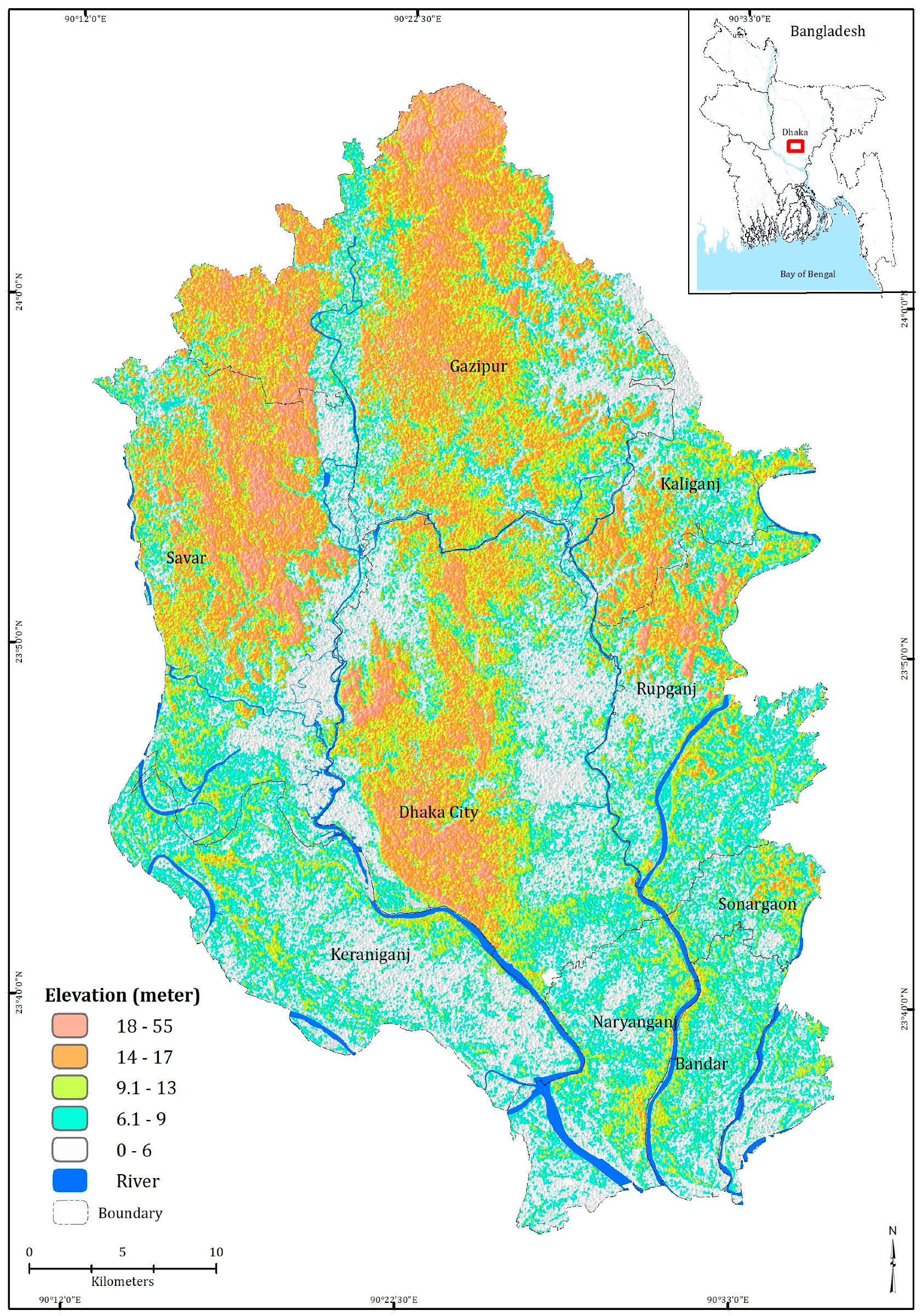
Figure 2.
The 20 most relative importance variables in descending order using the percentage of increase in mean squared prediction error: (A) 1990; (B) 1995; (C) 2000; (D) 2005; (E) 2010; (F) 2015.
Figure 2.
The 20 most relative importance variables in descending order using the percentage of increase in mean squared prediction error: (A) 1990; (B) 1995; (C) 2000; (D) 2005; (E) 2010; (F) 2015.
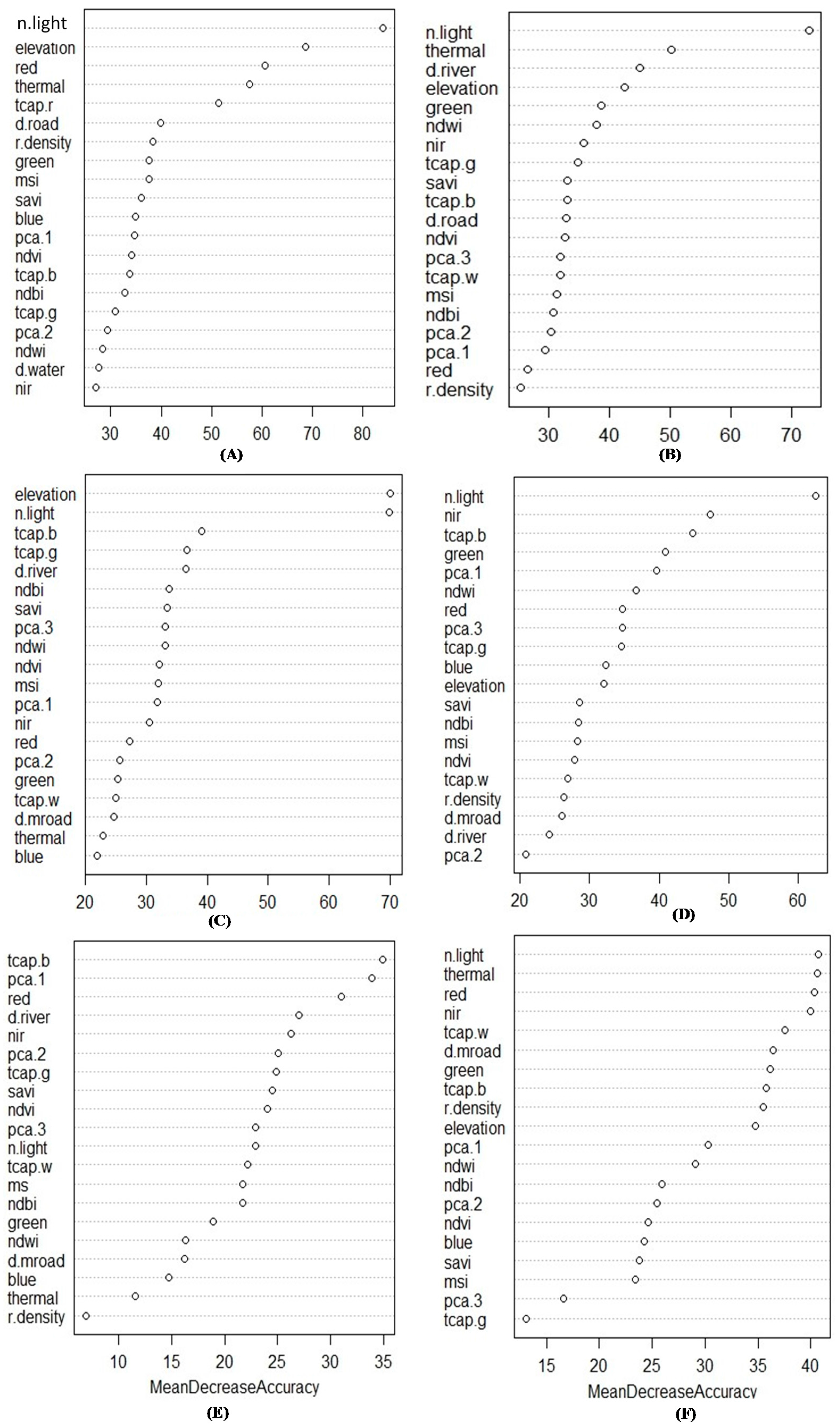
Figure 3.
Spatiotemporal distribution of land covers and patterns of urbanization in greater Dhaka from 1972 to 2015: (A) 2015; (B) 2010; (C) 2005; (D) 2000; (E) 1995; (F) 1990; (G) 1980; (H) 1972.
Figure 3.
Spatiotemporal distribution of land covers and patterns of urbanization in greater Dhaka from 1972 to 2015: (A) 2015; (B) 2010; (C) 2005; (D) 2000; (E) 1995; (F) 1990; (G) 1980; (H) 1972.
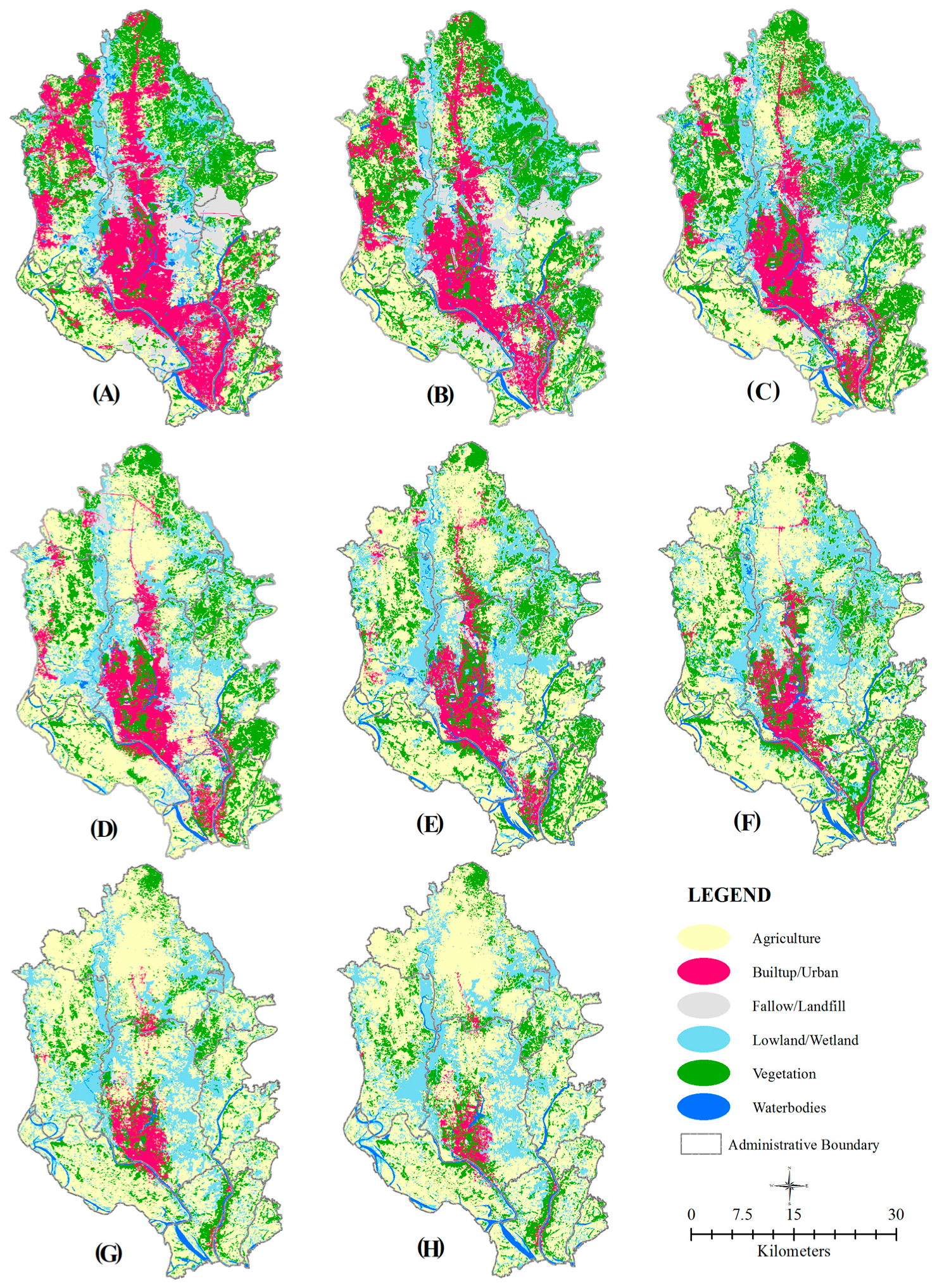
Figure 4.
The proportional distribution (%) of each land cover class in eight periods. (A) Core city area/Dhaka City Corporation area and (B) whole study area.
Figure 4.
The proportional distribution (%) of each land cover class in eight periods. (A) Core city area/Dhaka City Corporation area and (B) whole study area.
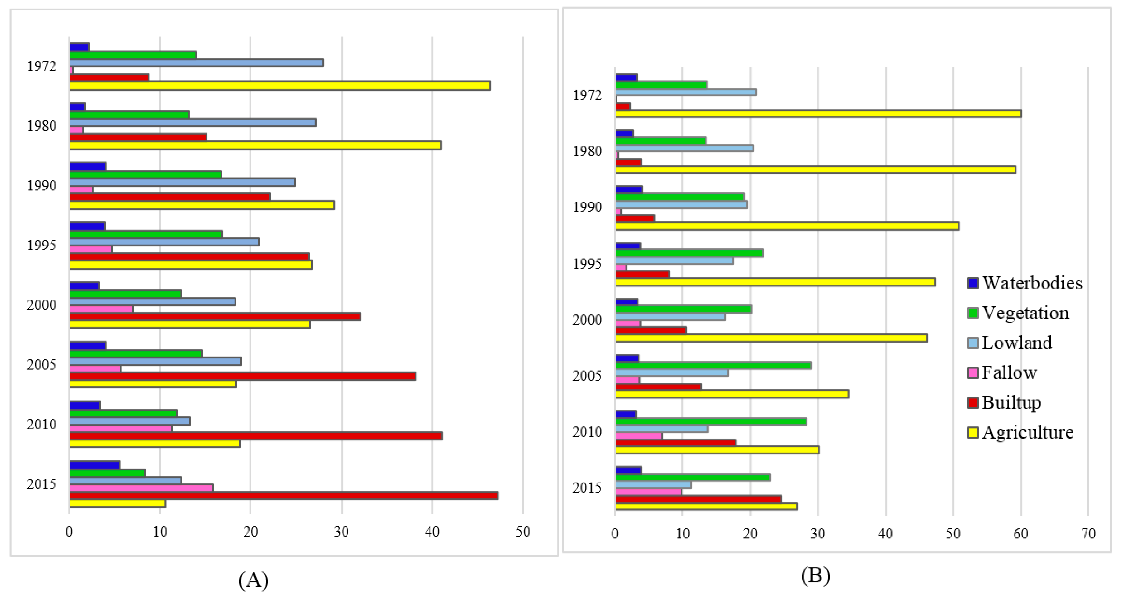
Figure 5.
Land cover map of the Core city/Dhaka City Corporation area (DCC) between 1972 and 2015. (A) 2015; (B) 2010; (C) 2005; (D) 2000; (E) 1995; (F) 1990; (G) 1980; (H) 1972.
Figure 5.
Land cover map of the Core city/Dhaka City Corporation area (DCC) between 1972 and 2015. (A) 2015; (B) 2010; (C) 2005; (D) 2000; (E) 1995; (F) 1990; (G) 1980; (H) 1972.

Figure 6.
Land use/land cover map of Savar from 1980 to 2015. Map: (A) 2015; (B) 2000; (C) 1990; and (D) 1980.
Figure 6.
Land use/land cover map of Savar from 1980 to 2015. Map: (A) 2015; (B) 2000; (C) 1990; and (D) 1980.

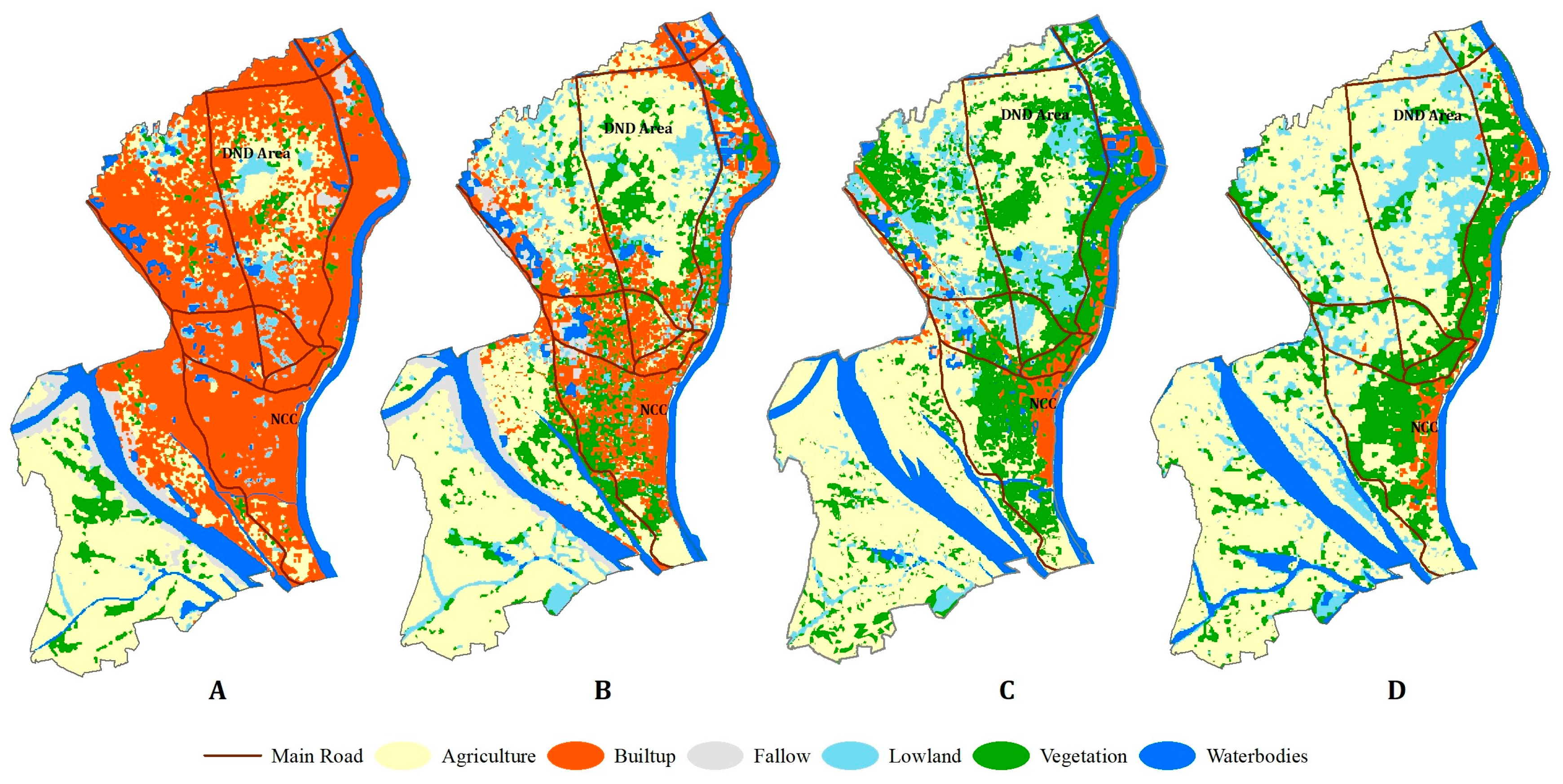
Figure 7.
Land use/land cover map of Naryanganj represents urban expansion for the years (A) 2015; (B) 2000; (C) 1990; and (D) 1980.
Figure 7.
Land use/land cover map of Naryanganj represents urban expansion for the years (A) 2015; (B) 2000; (C) 1990; and (D) 1980.

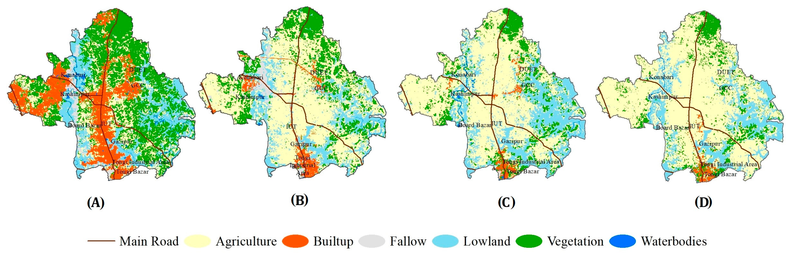
Figure 8.
Land cover map of Gazipur. (A) 2015; (B) 2000; (C) 1990 and (D) 1980.

Figure 9.
The spider diagram on the left represents spatial patterns of urban growth trajectories (in hectares) in 16 directions between 1972 and 2015. The map on the right shows recent urban growth trends in six major corridors. (A) Dhaka–Aricha Highway; (B) Savar–Ashluia–Baipayl; (C) Tongi–Gazipur along the Dhaka–Maymenshing Highway; (D) Dhaka–Chittagong Highway; (E) Dhaka–Narayanganj Road; and (F) Dhaka–Narayangang–Munshiganj corridors.
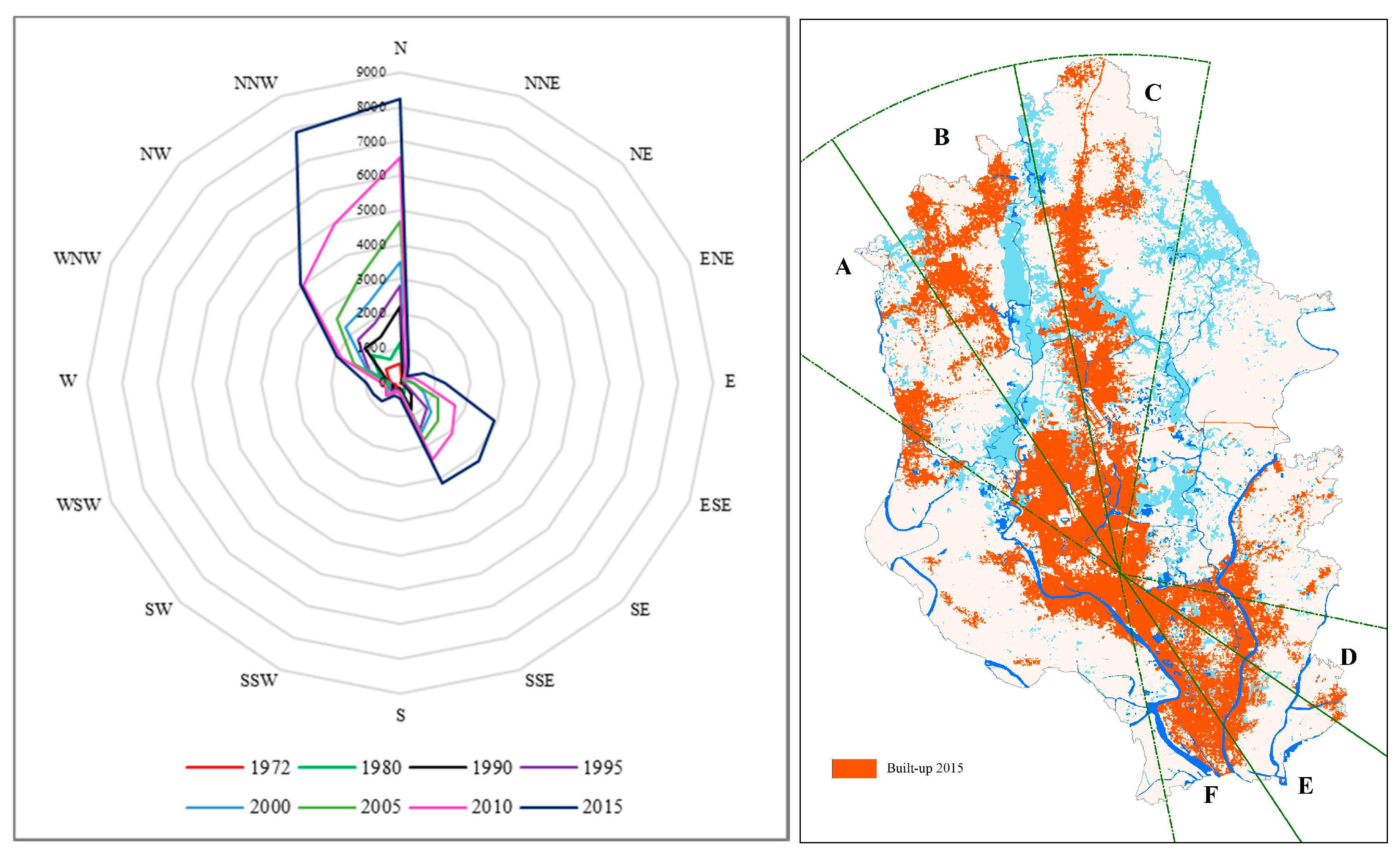
Figure 10.
The bar chart on the left (A) compares total built-up area between the core city (DCC) and the peripheral area and the line graph on the right (B) compares annual urban expansion rate (%) with annual urban population growth rate (%) from 1972 to 2015.
Figure 10.
The bar chart on the left (A) compares total built-up area between the core city (DCC) and the peripheral area and the line graph on the right (B) compares annual urban expansion rate (%) with annual urban population growth rate (%) from 1972 to 2015.

Table 1.
Descriptions of the major land cover categories.
| Land Cover Types | Description |
|---|---|
| Urban/Built-up area | These include all developed land, including commercial, residential, industrial, and other infrastructure |
| Agriculture/Crop field | Land used for agriculture, paddy field, vegetables, fruits, and other cultivable lands |
| Water bodies | Lake, ponds, lagoon, river, and aqua fishing |
| Forest and Vegetation | Hilly forest, bush and shrubs, settlements under tree cover, homestead vegetation |
| Landfill/Fallow land | Fallow land, uncultivated land, open hill, exposed soil, landfill, barren land, bare soil, sands, dunes and river banks, playgrounds and other restricted vacant land |
| Lowland/Wetland | Permanent and seasonal wetlands, marshy land, rills and gullies, swamps |
Table 2.
List of predictor variables and their descriptions. Topographic variables were derived from the SRTM 30 DEM. Spectral variables and spectral indices were computed using spectral bands of Landsat imagery of TM, ETM+, and OLI-TIRS.
Table 2.
List of predictor variables and their descriptions. Topographic variables were derived from the SRTM 30 DEM. Spectral variables and spectral indices were computed using spectral bands of Landsat imagery of TM, ETM+, and OLI-TIRS.
| Variable Type | Variable Name | Variable Description |
|---|---|---|
| Topographic Variables | Slope | Land slope extracted from SRTM 30-m DEM data |
| Elevation | Surface elevation above sea-level in meters calculated from a digital terrain model | |
| Aspect | Surface orientation calculated from DEM data | |
| Spectral Variables | Red Band | Spectral Value of Red Band |
| Green Band | Spectral Value of Green Band | |
| Blue Band | Spectral Value of Blue Band | |
| NIR Band | Spectral Value of Near Infrared Band | |
| Thermal Band | Spectral Value of Thermal Infrared Band | |
| DMSP-OLS | Spectral Signature of DMSP-OLS nighttime lights imagery | |
| Spectral Indices | NDVI | Normalized Difference Vegetation Index (NDVI) calculated as (NIR Band-Red Band)/(NIR Band + Red Band) |
| NDWI | Normalized Difference Water Index (NDWI) calculated as (Green Band-NIR Band)/(Green Band + NIR Band) | |
| NDBI | Normalized Difference Built-up Index (NDBI) calculated as; (SWIR-NIR)/(SWIR + NIR) | |
| MSI | Moisture Stress Index (MSI) calculated as; Mid Infrared/NIR | |
| SAVI | Soil Adjusted Vegetation Index (SAVI) calculated as; ((NIR-Red)/(NIR + Red + 0.5)) * 1.5)) | |
| TCAP-B | Tasseled Cap Analysis Brightness calculated as: (0.319 * Blue Band) + (0.542 * Green Band) + (0.490 * Red Band) + (0.604 * NIR Band) | |
| TCAP-G | Tasseled Cap Analysis Greenness calculated as: (−0.121 * Blue Band) − (0.331 * Green Band) − (0.517 * Red Band) + (0.780 * NIR Band) | |
| TCAP-W | Tasseled Cap Analysis Wetness calculated as: (0.652 * Blue Band) + (0.375 * Green Band) − (0.639 * Red Band) − (0.163 * NIR Band) | |
| PCA-1, PCA-2 and PCA-3 | Principal Component Analysis scores (first 3 PCA) calculated using all the Spectral Bands | |
| Infrastructure | Road Density | Road Density Scores calculated using line density function in ArcGIS |
| Distance to Main Road | Euclidian Distance from the main road calculated in ArcGIS | |
| Distance to River/Lake | Euclidian Distance from the main lake and river calculated in ArcGIS |
Table 3.
Accuracy assessment using independent reference points. UA: User Accuracy, PA: Producer Accuracy, OA: Overall Accuracy.
Table 3.
Accuracy assessment using independent reference points. UA: User Accuracy, PA: Producer Accuracy, OA: Overall Accuracy.
| 2015 | 2010 | 2005 | 2000 | 1995 | 1990 | 1980 | 1972 | |
|---|---|---|---|---|---|---|---|---|
| UA/PA | UA/PA | UA/PA | UA/PA | UA/PA | UA/PA | UA/PA | UA/PA | |
| Agriculture | 94/91 | 94/91 | 86/85 | 67/83 | 65/92 | 65/92 | 80/100 | 75/100 |
| Vegetation | 92/92 | 94/96 | 87/89 | 85/86 | 85/82 | 78/78 | 81/78 | 68/70 |
| Built-up | 91/96 | 92/92 | 96/92 | 98/90 | 96/88 | 93/84 | 94/88 | 93/78 |
| Lowland/Wetland | 94/94 | 96/94 | 89/92 | 71/74 | 75/78 | 67/70 | 80/74 | 60/63 |
| Fallow | 98/96 | 94/95 | 92/90 | 94/87 | 97/89 | 97/87 | 97/92 | 97/87 |
| Water bodies | 96/96 | 98/96 | 96/98 | 73/85 | 75/92 | 75/92 | 68/100 | 61/84 |
| OA | 94% | 97% | 91% | 85% | 86% | 89% | 86% | 87% |
| KAPPA | 0.93 | 0.94 | 0.89 | 0.81 | 0.82 | 0.87 | 0.82 | 0.84 |
Table 4.
Area statistics of each land cover category, total and annual increase/decrease rate in core city area (DCC) (Unit: Hectares and %).
Table 4.
Area statistics of each land cover category, total and annual increase/decrease rate in core city area (DCC) (Unit: Hectares and %).
| DCC | 1972 | 1980 | 1990 | 1995 | 2000 | 2005 | 2010 | 2015 | Increase/Decrease (Total %) | Increase/Decrease (Annual %) |
|---|---|---|---|---|---|---|---|---|---|---|
| Agriculture | 14,193 | 12,527 | 8958 | 8194 | 8142 | 5626 | 5762 | 3256 | −77 | −3 |
| Built-up | 2694 | 4643 | 6769 | 8105 | 9843 | 11,677 | 12,579 | 14,472 | 437 | 4 |
| Fallow/Landfill | 133 | 475 | 801 | 1444 | 2144 | 1729 | 3463 | 4867 | 3562 | 9 |
| Lowland/Water bodies | 9225 | 8854 | 8862 | 7601 | 6626 | 7020 | 5095 | 5479 | −41 | −1 |
| Vegetation | 4281 | 4027 | 5136 | 5183 | 3771 | 4474 | 3626 | 2451 | −43 | −1 |
Table 5.
Area statistics of each land cover class, total and annual increase/decrease rate in Savar (Unit: hectares and %).
Table 5.
Area statistics of each land cover class, total and annual increase/decrease rate in Savar (Unit: hectares and %).
| SAVAR | 1972 | 1980 | 1990 | 1995 | 2000 | 2005 | 2010 | 2015 | Increase/Decrease (Total %) | Increase/Decrease (Annual %) |
|---|---|---|---|---|---|---|---|---|---|---|
| 1972–2015 | 1972–2015 | |||||||||
| Agriculture | 14,580 | 14,764 | 14,265 | 13,043 | 12,614 | 7808 | 8029 | 8148 | −44.1 | −1.3 |
| Built-up | 40 | 93 | 148 | 628 | 1274 | 1861 | 4660 | 5071 | 12,576.4 | 11.9 |
| Fallow | 10 | 49 | 134 | 341 | 729 | 1116 | 1648 | 2092 | 20,825.5 | 13.2 |
| Lowland/Water bodies | 7543 | 7245 | 5950 | 7057 | 6147 | 6483 | 4094 | 4674 | −38.0 | −1.1 |
| Vegetation | 3186 | 3186 | 4839 | 4267 | 4572 | 8065 | 6906 | 5348 | 67.9 | 1.2 |
Table 6.
Area statistics of each land cover category, total and annual increase/decrease rate in Narayanganj (Unit: hectares and %).
Table 6.
Area statistics of each land cover category, total and annual increase/decrease rate in Narayanganj (Unit: hectares and %).
| Periods | 1972 | 1980 | 1990 | 1995 | 2000 | 2005 | 2010 | 2015 | Total Increase/Decrease (%) | Increase/Decrease (Annual %) |
|---|---|---|---|---|---|---|---|---|---|---|
| LUCC | 1972–2015 | 1972–2015 | ||||||||
| Agriculture | 5136 | 5200 | 4375 | 4275 | 4160 | 4220 | 3258 | 2370 | −53.8 | −1.8 |
| Built-up | 238 | 235 | 612 | 1633 | 1720 | 2217 | 3350 | 4880 | 1946.5 | 7.3 |
| Fallow | 2 | 5 | 131 | 244 | 435 | 335 | 411 | 410 | 23,910.6 | 13.6 |
| Lowland/Water bodies | 2331 | 2285 | 1847 | 1818 | 1881 | 1449 | 1427 | 1365 | −41.4 | −1.2 |
| Vegetation | 1790 | 1773 | 2531 | 1526 | 1301 | 1276 | 1051 | 472 | −73.6 | −3.1 |
Table 7.
Total built-up area (in hectares) in nine connecting cities from 1972 to 2015. The highest urban development in 43 years was documented in the core city area (DCC) and the lowest was in Kaliganj.
Table 7.
Total built-up area (in hectares) in nine connecting cities from 1972 to 2015. The highest urban development in 43 years was documented in the core city area (DCC) and the lowest was in Kaliganj.
| Urban/Built-Up (ha) | 1972 | 1980 | 1990 | 1995 | 2000 | 2005 | 2010 | 2015 |
|---|---|---|---|---|---|---|---|---|
| Dhaka City | 2600 | 4600 | 6882 | 8246 | 9931 | 11,738 | 12,637 | 14,523 |
| Gazipur | 243 | 596 | 818 | 1434 | 1684 | 2277 | 4554 | 7640 |
| Savar | 40 | 93 | 148 | 628 | 1274 | 1861 | 4660 | 5071 |
| Narayanganj | 238 | 335 | 612 | 1633 | 1720 | 2217 | 3350 | 4880 |
| Keraniganj | 138 | 241 | 296 | 338 | 539 | 557 | 629 | 1952 |
| Bandar | 98 | 115 | 152 | 196 | 482 | 579 | 667 | 1532 |
| Rupganj | 3 | 9 | 53 | 76 | 197 | 231 | 627 | 1288 |
| Sonargaon | 10 | 30 | 40 | 70 | 185 | 204 | 278 | 851 |
| Kaliganj | 0 | 1 | 1 | 1 | 3 | 5 | 6 | 6 |
© 2017 by the authors. Licensee MDPI, Basel, Switzerland. This article is an open access article distributed under the terms and conditions of the Creative Commons Attribution (CC BY) license (http://creativecommons.org/licenses/by/4.0/).
Share and Cite
MDPI and ACS Style
Hassan, M.M.; Southworth, J. Analyzing Land Cover Change and Urban Growth Trajectories of the Mega-Urban Region of Dhaka Using Remotely Sensed Data and an Ensemble Classifier. Sustainability 2018, 10, 10. https://doi.org/10.3390/su10010010
AMA Style
Hassan MM, Southworth J. Analyzing Land Cover Change and Urban Growth Trajectories of the Mega-Urban Region of Dhaka Using Remotely Sensed Data and an Ensemble Classifier. Sustainability. 2018; 10(1):10. https://doi.org/10.3390/su10010010
Chicago/Turabian StyleHassan, Mohammad Mehedy, and Jane Southworth. 2018. "Analyzing Land Cover Change and Urban Growth Trajectories of the Mega-Urban Region of Dhaka Using Remotely Sensed Data and an Ensemble Classifier" Sustainability 10, no. 1: 10. https://doi.org/10.3390/su10010010
Note that from the first issue of 2016, this journal uses article numbers instead of page numbers. See further details here.