An Algorithm for Modelling the Impact of the Judicial Conflict-Resolution Process on Construction Investment

Abstract

In this article, the modelling of the judicial conflict-resolution process is considered from a construction investor’s point of view. Such modelling is important for improving the risk management for construction investors and supporting sustainable city development by supporting the development of rules regulating the construction process. Thus, this raises the problem of evaluation of different decisions and selection of the optimal one followed by distribution extraction. First, the example of such a process is analysed and schematically represented. Then, it is formalised as a graph, which is described in the form of a decision graph with cycles. We use some natural problem properties and provide the algorithm to convert this graph into a tree. Then, we propose the algorithm to evaluate profits for different scenarios with estimation of time, which is done by integration of an average daily costs function. Afterwards, the optimisation problem is solved and the optimal investor strategy is obtained—this allows one to extract the construction project profit distribution, which can be used for further analysis by standard risk (and other important information)-evaluation techniques. The overall algorithm complexity is analysed, the computational experiment is performed and conclusions are formulated.

1. Introduction

In this article, it is considered how society rights violations may affect the implementation of a construction investment project. The infringement of society rights can be harmful to investors, since the judicial process can greatly increase the costs of the project and reduce the profit or even make it negative. On the one hand, it is important to avoid conflicts that can greatly increase the costs of the construction investment project or even force it to stop. On the other hand, in the case when the judicial process is avoided, some slight violations may greatly reduce the construction project’s costs or increase its value, leading to increased profit for construction investors. Thus, investors should make some decisions carefully during the preparation of the project. For a project’s successful execution, it is crucial to evaluate and manage risk factors in cases of different decisions. The correct decision strategy for a conflict-resolution process would minimise risks or costs. More generally, it is needed to choose the ratio between risks and costs. Usually, investors underestimate the risks, and thus the correct strategy selection made by construction investors leads one to avoid conflicts, which leads to avoidance of project failures and makes a great deal for sustainable city development. However, even if the optimal decision strategy is known, it is important to evaluate the project, since at the project initialization stage, such an evaluation helps one to select the most suitable project from all possible alternatives or to refuse to start any projects at all. Nowadays, planning and management technologies can greatly improve the quality of investor decisions. Integration of such technologies into project implementation is very significant for investors.

Investment efficiency plays a critical role in investment prioritisation, and therefore, it has become an important topic in recent research [1,2]; the irreversibility of potential negative outcomes of projects was studied [3], and the optimal project portfolio creation was studied [4]. There exist methods for supporting investments and resource allocation in risky environments (see [5]). The investment-supporting methods are important in the construction field; for example, a contractor’s selection can be supported by special methods [6,7]. Special problems are formulated and solved for assessment of unfinished construction projects [8]. The problem of optimal project selection can be very complex due to the risks associated with uncertainties in the projects, which should be properly addressed [9]. Some risks are highly related to conflicts between decision makers; for example, a recent study addressed the conflict between a construction company and selected suppliers [10]. However, there are no studies dedicated to evaluate the project from the perspective of risks that come from the judicial process that arise from some slight law violations that were made purposely. In this paper, we develop an algorithm that is aimed to help investors to manage the risks that are connected to the judicial conflict-resolution process, that is, an algorithm for modelling the impact of the judicial conflict-resolution process on construction investment.

In this paper, we concentrate on a specific case when the problem is defined by a graph with cycles, and some natural properties of the problem can be used to obtain a tree. Another important result of this work is formal representation of such a process with estimation of time and decision cycles. More specifically, the investment into construction of buildings is considered. In our case, decisions that should be made are dependent on the past (i.e., after some cycles it depends on which state it was in before), so initially it is not a Markov decision process [11]. However, during the execution of the proposed algorithm, it eventually becomes a Markov decision process, and, after the optimal strategy is selected, the process becomes a Markov chain. When the problem is formulated in the form of the Markov chain, there are many ways to solve it [12]. However, in this paper we consider this problem as a general problem on graphs. Since the Markov decision process structure is described by a tree, the solution of the considered problem is easy to find—we provide algorithms to solve it.

The practical importance of the analysis of the investment in building construction processes is well described in [13]. This forces companies to build on the limits of construction law restrictions and sometimes they even slightly violate the law. Some non-critical construction law violations can be widely found in construction projects that are already successfully finished [14]. In this situation, we are inclined to blame the drawbacks of laws that regulate urban planning and protection of visual identity (investors cannot always be expected to abandon their self-centred ends for the sake of urban values, etc.). This is largely influenced by confusing, non-effective systems for the coordination with government institutions and the public. The regulation of construction is confusing, and the builders breach the introduced requirements. Inappropriate distribution of functions among government institutions and private subjects raises a lot of problems. One of the outcomes of inappropriate legal regulation is violation of the society’s rights (i.e., the parties that are not directly related to the investment construction process, owners of neighbouring plots, users, communities of residential districts, etc.). Even if the construction is done without any violations of the procedures, negative impact on the surrounding environment may exist. This can be described as social cost in construction projects, and a state-of-the-art overview of social costs in the construction industry is presented in [15].

It may seem that a smart decision to make the law violations protects the interests of investors only. However, the investors may violate the law purposely in some cases only, and in other cases the modelling of processes would objectively indicate that breaking the law is not profitable—this would contribute to sustainable city development. More specifically, it is profitable to violate the law in the case when the risks of the conflict between the construction company and the society are small compared to the rewards. Obviously, if the potential profit is big, the investors would make decisions that lead to a high probability of the conflict. In this case, such an investment strategy stands against the higher degree of sustainability of city development. Thus, the proposed algorithm can be used to identify the cases when the behaviour of the investors may contribute to unsustainable development. Additional analysis of such cases would lead one to identify the rules that do not regulate the construction process strictly enough. An example of such a detailed analysis of territorial planning procedures is provided in [16], where a detailed description of Lithuanian laws and its regulating system can be found. The application of this research could contribute to the sustainable city development in two ways: by stopping the investors from taking risks that will probably lead to the conflict with society (leading to loses), and by indicating the drawbacks of the regulatory system when the law violations (i.e., risks) are profitable. In the first case, such modelling would prevent the investors from taking socially destructive actions (i.e., violation of the law). In the second case, it would work in two ways: it would encourage the investors to violate the law, and indicate that the regulation procedures must be modified to make the expected penalties large enough (in terms of probability of identifying the violations by inspecting institutes and the size of fines) to make it not profitable to violate the law. Thus, we assume that such modelling could be used (along with the investors) by institutions that control the development of territorial planning procedures. It is especially important in the case when the investor chooses to violate some critical laws, such as ones that are related to toxic waste [17]. The distinction between more and less important (in some sense) laws is out of the scope of the current research—it must be analysed in each case separately. However, the application of this research can indicate in which cases such analysis must be performed.

The modelling of such a process was already performed in [13,14], and was done using recurrence equations that were solved using the dynamic programming concept. However, the proposed method is limited to the decision tree, thus it does not support cycles. Moreover, it solves the fixed optimisation problem, which gives a limited amount of information. For example, it can give the average profit value, but cannot give any information on the risks of losing a large amount of invested money. These results were extended in [18,19], where the conceptual model was applied to describe the behaviour of two conflicting systems (the investor and community) in different states and times. It revealed the importance of duration of different events during a judicial conflict-resolution process and showed how to estimate it and include in the model. As a consequence, it became possible to estimate cycles in the graph that describe the process—this can be an important part of project evaluation. However, such modelling of judicial process resolution with estimation of time and cycles was not performed before, and this is what this research is dedicated to.

The main aim of this research is to perform the evaluation of the judicial conflict-resolution process’s impact on investment with estimation of time and decision cycles. More specifically, the authors develop an algorithm that allows one to extract the project’s profit distribution semi-automatically. The probability of occurrence of different events in different states must be evaluated by experts or by other means, as well as the whole set of events and the set of dependencies between these events—we assume that this data is known; for considered cases this data is partially taken from other publications. As for parameter estimation from empirical data—sometimes it is even possible to develop the patterns describing judicial decisions; in a recent research a large collection of judicial cases was used to measure the probabilities quite precisely [20]. It is important to note that the sensitivity analysis is out of the scope of this research; for example, probability values can be perturbed in order to gather more general results that are robust to errors of estimation of probability values in a similar way to what was done by other authors [21,22]. Some recent studies propose a comprehensive sensitivity analysis to identify the uncertain parameters that significantly influence the decision-making process in investments, and quantify their degree of influence [23].

The research topic deals with strategic management; it is strongly related to agency [24] and stakeholder [25] theories. According to the agency theory, the investor can be represented as a principal, and the construction company as an agent. One of problems being addressed in the agency theory is different risk toleration by a principal and an agent. The construction company (compared to the investors) may be less sensitive to a project failure, because the financial losses are not direct—they depend on contract clauses, the impact on reputation of the company [26], and so on. As for the investor—he loses the invested money directly as the project fails and stops. Thus, we assume that the construction company and the investors have different attitudes towards the risk of project failure. The proposed modelling supports the interests of the investors; these interests overlap with interests of society, and contribute to sustainable city development. In other words, this research contributes to the increase of investment protection; it can also affect corporate social responsibility for construction companies. The impact of investors’ protection on the company earnings management was analysed in recent research [27]. The stakeholder theory considers the will of an organisation to be directly affected by interests of different stakeholders. According to that theory, the society and the investors are external stakeholders of the organisation (construction company). In this case, the investors are shareholding stakeholders. In the stakeholder theory, the business decisions are usually optimised from the point of view of a business organisation (construction company)—optimisation is done taking into account the interests of all stakeholders. In this paper, we concentrate on the optimisation of decision strategy according to the interests of the investors. Thus, this research contributes to the stakeholder theory by investigating the risks taken by the investors. It is important to note that this does not mean that the investors are aware of the risks and will act according to them—the risks for the investors can be partially neglected by the construction company; however, according to stakeholder theory, the construction company should care for the interests of the investors. In recent work, there was performed an experimental scenario study in which investment behaviour was analysed in situations when management had to make trade-offs between shareholders’ and non-shareholding stakeholders’ interests [28]. In a similar way, the modelling proposed in this paper can potentially be applied to model the behaviour of the investors and their reactions to construction company decisions.

This research is dedicated to show how to model judicial processes and their impact; that is, it is focused on algorithms for computer simulation. This paper makes the following contributions. (1) We investigate the modelling of the investors’ behaviour that impacts the sustainability of the city development. The developed algorithm can be applied as a tool in other research in order to identify the drawbacks of the regulatory system and to evaluate impacts of regulation changes. Assuming that the investors take the risks that are too big, such modelling can help the investors to avoid socially destructive actions—law violations that would lead to judicial conflicts. If the risks are recommended to be taken, it would indicate that more investigation of some cases may be needed to evaluate the negative consequences of such violations on the sustainability. (2) We propose a modelling approach to evaluate the impact of the judicial conflict-resolution process on the investment. The model was based on another work [13], where the modelling was very limited to a specific case, which lacked the flexibility (without time or cycle estimation) and formalised algorithmic representation. (3) It provides the algorithm that lets one estimate the time and cycles (cyclic repeat of the events), giving a big variety of applications for similar process-modelling problems. Moreover, we propose a simple algorithm to calculate cost and time parameters for different scenarios (in [13], it was assumed to be known without any formal calculation procedure). (4) It provides the algorithms to simulate the impact of the judicial conflict-resolution process on the investment, when the costs of failure depend on time. More specifically, it shows how to extract the profit distribution from the model. This simulation result lets one evaluate different projects and compare them. (5) It shows how to model the Markov decision process (that is a part of the considered problem) using the algorithms on a tree that are represented from the perspective of the general theory of algorithms, independently from approaches that are usually used in these cases. The algorithms are represented in a simple-to-understand form as a recursion. Greedy algorithm and dynamic programming techniques are used.

This paper is organised as follows. In Section 2, we present an example of the process of judicial conflict resolution. In accordance with this example, we identify aspects that are important for the model, and in Section 3 propose the data structure that is suitable to describe the information that is needed for the algorithms. In Section 3, we propose a solution in the form of a set of algorithms. In Section 4, we apply these algorithms to the example from Section 2. The conclusions are formulated in Section 5.

2. Example and Problem Formulation

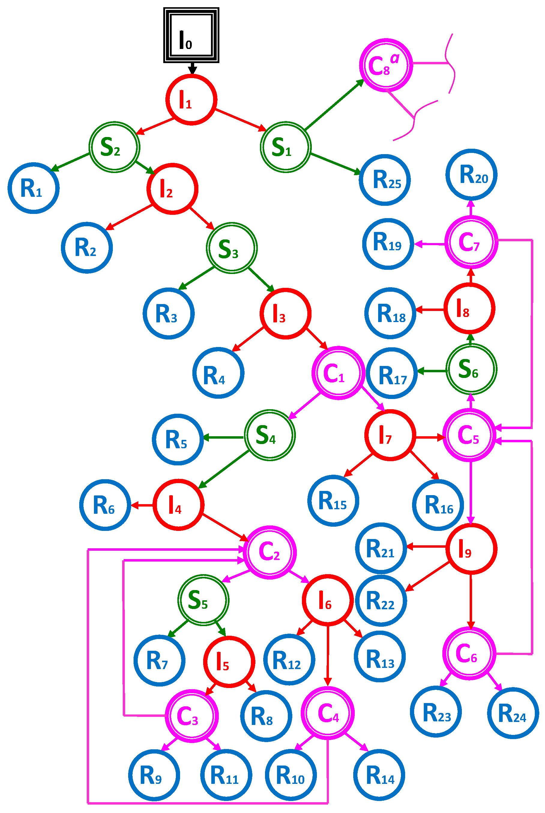
In this section we consider an example of the process of judicial conflict resolution that was already described before in [13,14]. This process is related to an investment project of a residential building that is located in Vilnius (Lithuania) at the address Seskines 45C [29]. In this section we will present only some details of this process. There are three sides involved in a conflict—the investor, the society and the court. We will refer to these sides by abbreviations $I_{k_1}$ (investor), $S_{k_2}$ (society) and $C_{k_3}$ (court), where $k_1,k_2,k_3$ are the identification numbers of different events in which decisions are made by different sides. The whole process is represented by the decision graph (Figure 1), in which decision nodes are $I_{k_1}$, chance nodes are $S_{k_2}$ and $C_{k_3}$, and the end nodes are $R_{k_4}$. $R_{k_4}$ represent the judicial conflict-resolution scenarios.

The description of graph edges is presented in

Table 1. The description of the conflict participants’ behaviour, and the losses due to the judicial process. Costs are presented in TEUR (thousands euros); $I,S,C$ denotes the Investor, the Society and the Court, respectively. R denotes the Result nodes (the ends of scenarios).

Edge	Actions (Decisions) Description	t (Days)	p	Losses (TEUR)
$(I_0,I_1)$	Project begins	0	$x_{0,1}$	0
$(I_1,S_2)$	I informs S (according to law)	180	$x_{1,1}$	0
$(I_1,S_1)$	I informs S (violates the law)	630	$x_{1,2}$	0
$(S_2,R_1)$	S does not submit its suggestions	30	0.8	0
$(S_2,I_2)$	S submits its suggestions	14	0.2	0
$(I_2,R_2)$	I accepts suggestions	14	$x_{2,1}$	1000
$(I_2,S_3)$	I rejects suggestions	14	$x_{2,2}$	0
$(S_3,I_3)$	S applies to an advanced hearing institution	7	0.7	0
$(S_3,R_3)$	S does not apply to an advanced hearing institution	30	0.3	0
$(I_3,R_4)$	I makes a peace treaty with S	14	$x_{3,1}$	150
$(I_3,C_1)$	I does not make a peace treaty with S	21	$x_{3,2}$	10
$(C_1,S_4)$	I loses	30	0.4	0
$(C_1,I_7)$	I wins	30	0.6	0
$(S_1,C_8)$	S applies to an advanced hearing institution	28	0.1	0
$(S_1,R_{25})$	S does not apply to an advanced hearing institution	30	0.9	0
$(S_4,R_5)$	S does not apply to a court of first instance	14	0.25	$-10$
$(S_4,I_4)$	S applies to a court of first instance	7	0.75	0
$(I_4,C_2)$	I does not make a peace treaty with S	7	$x_{4,2}$	20
$(I_4,R_6)$	I makes a peace treaty with S	7	$x_{4,1}$	100
$(C_2,S_5)$	I wins	90	0.5	0
$(C_2,I_6)$	I loses	90	0.5	0
$(S_5,R_7)$	S does not apply to a court of appeal	14	0.15	$-30$
$(S_5,I_5)$	S applies to a court of appeal	7	0.85	0
$(I_5,C_3)$	I does not make a peace treaty with S	7	$x_{5,2}$	10
$(I_5,R_8)$	I makes peace treaty with S	7	$x_{5,1}$	100
$(C_3,R_9)$	I wins	120	0.35	$-40$
$(C_3,R_{11})$	I loses	120	0.35	0
$(C_3,C_2)$	C returns a lawsuit to a court of first instance	120	0.3	0
$(I_6,R_{13})$	I does not apply to a court of appeal	14	$x_{6,1}$	0
$(I_6,C_4)$	I applies to a court of appeal	14	$x_{6,2}$	10
$(I_6,R_{12})$	I makes a peace treaty with S	14	$x_{6,3}$	200
$(C_4,R_{14})$	I loses	120	0.35	0
$(C_4,C_2)$	C returns a lawsuit to a court of first instance	120	0.3	0
$(I_7,R_{16})$	I does not apply to a court of appeal	14	$x_{7,1}$	0
$(I_7,C_5)$	I applies to a court of first instance	14	$x_{7,2}$	20
$(I_7,R_{15})$	I makes a peace treaty with S	14	$x_{7,3}$	150
$(C_5,S_6)$	I wins	90	0.5	0
$(C_5,I_9)$	I loses	90	0.5	0
$(S_6,R_{17})$	S does not apply to a court of appeal	14	0.15	$-30$
$(S_6,I_8)$	S applies to a court of appeal	7	0.85	0
$(I_8,C_7)$	I does not make a peace treaty with S	7	$x_{8,2}$	10
$(I_8,R_{18})$	I makes a peace treaty with S	7	$x_{8,1}$	100
$(C_7,R_{20})$	I wins	120	0.35	$-40$
$(C_7,R_{19})$	I loses	120	0.35	0
$(C_7,C_5)$	C returns a lawsuit to a court of first instance	120	0.3	0
$(I_9,R_{22})$	I does not apply to a court of appeal	14	$x_{9,1}$	0
$(I_9,C_6)$	I applies to a court of appeal	14	$x_{9,2}$	10
$(I_9,R_{21})$	I makes a peace treaty with S	14	$x_{9,3}$	200
$(C_6,R_{24})$	I wins	120	0.35	$-40$
$(C_6,R_{23})$	I loses	120	0.35	0
$(C_6,C_5)$	C returns a lawsuit to a court of first instance	120	0.3	0
$(C_4,R_{10})$	I wins	120	0.35	$-40$

with time values, costs and chance node probabilities or decision variable abbreviations. All money costs are measured in TEUR (thousands euros), time is measured in days. Some data was originally provided in Lithuanian litas—we converted it to euros by dividing by a factor 3.4528, and for simplicity performed some rounding off. For decision nodes the variables are denoted $X_{ij}$, which can be 1 or 0; i is the index of the investor node $I_i$ in which the decision is made; j is the number of decisions in this case. This means that for each i, values $X_{ij}$ are equal to 1, and remaining values are equal to 0.

The description of different ending scenarios is provided in

Table 2. The description of possible conflict endings.

End Nodes	Description	Success
$R_1,R_3,R_{25}$	successful completion of the judicial conflict	yes
$R_2$	project solution is changed, costs are increased	yes
$R_4,R_6,R_8,R_{12},R_{15},R_{18},R_{21}$	peace treaty is signed	yes
$R_5,R_7,R_9,R_{10},R_{17},R_{20},R_{24}$	investor wins the judicial conflict	yes
$R_{11},R_{13},R_{14},R_{16},R_{19},R_{22},R_{23}$	project failure	no

. However, it is unclear what are the actual profits (positive or negative) in different scenario cases—it depends on the graph (Figure 1).

To estimate costs, we use data from documents that are related to this investment project. Reference [30] is used to estimate the building price for sale by accumulating the quadrature of apartments (which is equal to 5998.8 m²) and multiplying it by its market value in 2007 taken from [31], which is mentioned to be from 1.39 to 2.17 TEUR, and for simplicity we assume that it is 1.5 TEUR per square metre. Thus, the estimation of the price the building was sold for gives 8998.2 TEUR. The building costs data is taken from [32] and is equal to 5508.6 TEUR. We note that we do not expect to estimate the needed data precisely—we consider this example for tests and demonstration purposes only, as our goal is to provide the algorithm for those who have access to this type of data directly. The building price and its distribution in time is important in order to estimate the amount of possible losses in the case when the investor loses the judicial process and fails to complete the project. Unfortunately, we do not have the exact data of the project’s cost distribution in time. However, we have the information on costs of the project that were paid before the judicial process was started—these costs were equal to 236.04 TEUR [33]. We use this number as project costs during the first phase of a project, which lasted for 613 days. The rest of $5508.573-236.04032$ we distribute as follows. We assume that the project costs in TEUR per day are higher at the beginning of the building process by 50% compared to the last phase of the building process due to additional costs of expensive machinery (cranes, etc.). The calculated data is used to compute average daily costs for different time intervals.

In

Table 3. The description of different project phases.

The Phase	Begin Date	End Date	Duration (Days)	Average Daily Costs (TEUR/Day)
1	1 October 2003	5 June 2005	613	0.3851
2	6 June 2005	4 September 2005	90	12.9018
3	5 September 2005	27 December 2006	478	8.6012
4	28 December 2006	28 April 2008	487	0

, we provide the interval lengths and average daily costs measured in TEUR per day for different project phases. Phase 1 is the phase before the actual building process has begun. Phases 2 and 3 describe the actual construction process; we separate the process into these phases taking into account that the project costs per day are higher at the beginning of the building process. Phase 4 describes the phase where the judicial process can be continued, however, the house construction is finished. The length of the first phase $l_1$ is taken from [19], the total cost is taken from [33] (as was mentioned before). The average daily costs parameter for phase 1, $c_1$, is calculated by dividing the total costs by $l_1$. The lengths for last two phases $l_2,l_3$ are taken as 90 and 478 days (the estimation for total length $l_2+l_3$ is taken from [32]) and the average daily costs $c_2,c_3$ are derived from the requirements $l_1{c}_1+l_2{c}_2+l_3{c}_3=5508.573$ and $c_2=1.5c_3$. The average daily costs are presented in Table 3. From this data we construct the average costs function $F\left(t\right)$ (Figure 2):

$$F\left(x\right)=\left\{\begin{array}{cc}0.3851,\hfill & 0\le t\le 613\\ 12.9018,\hfill & 613<t\le 703\\ 8.6012,\hfill & 1181<t\le 1668\\ 0,\hfill & 1668<t.\end{array}\right.$$

(1)

As was mentioned before, our goal is to provide an algorithm to extract the project profit distribution.

First of all, there is a degree of freedom for the investor, since in some situations he can make decisions on his own—as was mentioned before, there exist decision nodes $I_k$. Each decision node has a set of undefined probabilities $X_k=\{x_{k,j},j=1,\cdots ,m_k\}$. We define the investment strategy as a set of all graph decisions $X=\{X_k,k=1,\cdots ,M\}$. The investment strategy must be chosen before the project evaluation is performed. There are different ways to choose the optimal strategy for the considered project, and one of the simplest ways to do that is to solve the optimisation problem

$$\underset{X}{max}{P}_0\left(X\right),$$

(2)

where $P_0\left(X\right)$ is a function that computes the expected profit value for root node with number 0, and in the general case for each node n the expectation value is defined by a classical probabilistic expectation value formula

$$P_n\left(X\right)=\sum _{i\in children\left(n\right)}{P}_i\left(X\right)·p_{n,i},$$

(3)

where $children\left(n\right)$ returns the list of children indexes for the node with index n, $p_{n,i}$ is the probability for the node with number i to follow after the node with number n. However, there are no restrictions for the $P_n$ computational algorithm (algorithmic form is presented in Section 3), for example, if for risk evaluation purposes it is needed to avoid big loses, additional weights or nonlinear functions may be used. Moreover, it can be integrated into a business-intelligence system, followed by prediction of business-intelligence system effectiveness (see [34]) in order to select the appropriate technique. The Bellman [35] principle gives the rule of optimal strategy, which states that in the case when the graph is a tree, (2) is fulfilled when X is chosen such as

$$\underset{X}{max}{P}_n\left(X\right)\forall n,$$

(4)

which means that we can apply the dynamic programming principle and begin the computation from the bottom of the tree, where the values $P_n$ are known. However, in our case we cannot apply the dynamic programming principle directly, because we have cycles in a graph (Figure 1). So firstly, we must convert the graph into a tree with some assumptions. We should note that our graph can be interpreted as a tree with some exceptions—edges that form cycles. More specifically: $(C_3,C_2)$, $(C_4,C_2)$, $(C_6,C_5)$, $(C_7,C_5)$. The main assumption is based on the real meaning of these edges—these edges mean the process is returning to the first-instance court. In our graph, it was assumed that the first-instance court event can be repeated indefinitely; however, in reality, a court of appeal usually avoids repeating this event many times. Thus, naturally, we assume the maximum repeat count for this event to be 2. Note that we do not provide any proof for the optimal maximum of the event repeat count to be 2, since our algorithm supports any positive integer value. This assumption lets us convert the considered graph into a tree, since we can recursively make copies of the subgraph from the nodes the process returns to.

$P_n$ for end nodes (leaves) can be calculated by accumulating the project costs and times from the top of the tree to the bottom, and computing the profit at the end nodes using a pre-order tree-traversal algorithm idea, the exact algorithm of which will be presented in Section 4. Time must be converted to costs at success and failure nodes in different ways. In the case of success, all costs of the whole building project must be measured and subtracted from sale income (as we mentioned, we consider it to be 8998.2 TEUR). For failure nodes, the building costs must be measured up to the moment of failure.

To choose the optimal strategy, we use (2) and (3). After this, we can evaluate the project by extracting the scenario profit distribution from the tree.

3. The Data Structure and the Algorithms

Firstly, we declare the data structure that will be sufficient to store all data needed. Edges in Figure 1 represent decisions, and nodes represent events that occur after decisions are made. Assuming that there are no cycles in a graph (it is a tree), we let each node correspond to the directional edge that points to that node (i.e., end node of the edge). The data of all edges can be stored in nodes, so we can represent the whole process as a tree.

Each event has the price value and the time value. In our approach, the price value represents the price of that event, that is, the actual price needed to perform the decision. However, the time value represents the time needed to pass before the event starts. This allows us to store all information from the considered example into a decision tree.

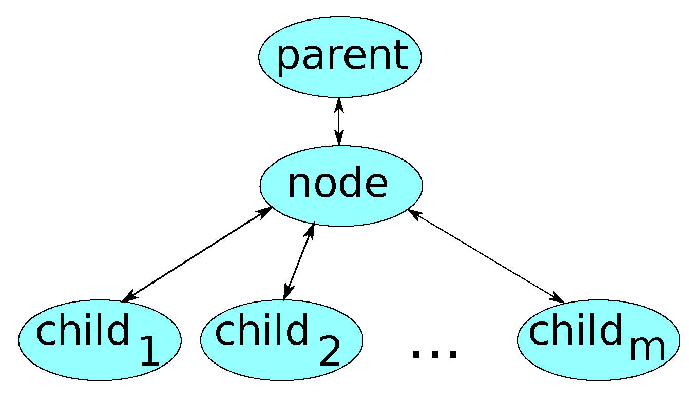
Thus, the basic element of our data structure (a tree) is a node with connections to parent and children nodes (Figure 3).

A more detailed description is presented in Algorithm 1, where the symbol “//” denotes comments that describe the corresponding fields. Field $type$ describes the type of a node. For our purposes, it is enough to define these types:

• 2—unsuccessful scenario end node,
• 1—investor decision node,
• 0—other nodes.

Note that types 1 and 2 are mutually exclusive, so we can use one field to describe this information. Field $cycle$ is the pointer that forms a cycle. We assume that if this pointer is not equal to $NULL$, then this node describes the edge to return to one of the previous events; we refer to it as cycle node. Here, we present some notes for such nodes:

• The node is fictive, that is, it must be added to the list of nodes to describe the additional edge (since in a graph there is more than one edge pointing to the same node).
• The node has no children—it is reserved to describe the parameters of an edge forming a cycle.
• After cycles are converted to the extended tree, such nodes must be deleted if they are leaves of the tree; the probabilities must be recalculated with the same proportions but without cycle nodes.

Algorithm 1: Data structure

struct {

int type; //node type

float p; //the probability for this node to be selected by parent

float price; //the price of event

float time; //the time before event starts

node* parent; //the pointer to parent node

vector< node* > children; //the list of children

node* cycle; //the pointer to the ancestor that forms a cycle

float priceTotal; //accumulated price

float timeTotal; //accumulated time

float value; //node expected profit value

} node;

Note, that in all presented functions it is assumed that the arguments are passed by reference, i.e., the changes of arguments are seen outside of these functions. We propose the algorithm that consists of these steps:

• Recursively make copies of the subgraph from nodes the process is returning to (i.e., looking for the pointer $cycle$), extend the tree by adding additional nodes. For this purpose we define a function $Expand$ in Algorithm 2.

  Algorithm 2: Cyclic expansion algorithm

  Function $Expand\left(node\right)$

  if $node.cycle!$ = NULL then

  if $depth<{depth}_{max}$ then

  $newNode=CopyOfSubtree(node.cycle)$

  $newNode.p=1$

  $newNode.parent=node$

  $node.children.add\left(newNode\right)$

  $depth=depth+1$

  $Expand\left(newNode\right)$

  $depth=depth-1$

  else

  // deletes unneeded fictive node and recalculates the probabilities

  // of parent’s children nodes leaving the same proportions

  smartDelete(node)

  end

  else

  for each node t in $node.children$ do

  Expand(t)

  end

  end

  end

• Calculate total times (field $timeTotal$) and costs (field $priceTotal$) up to the moment when events are finished—this is implemented in the function $CalcPars$ in Algorithm 3.
• Evaluate end-node scenarios (calculate field $value$) and select optimal strategy—function $CalcValues$ in Algorithm 4.
• Create profit (field $value$) distribution by calculating different scenario probabilities. A simple implementation is provided in Algorithm 5.

  Algorithm 3: Costs parameters calculation algorithm

  Function $CalcPars\left(node\right)$

  if $node.parent$ = NULL then

  $node.timeTotal=node.time$

  $node.priceTotal=node.price$

  else

  $node.timeTotal=node.time+node.parent.timeTotal$

  $node.priceTotal=node.price+node.parent.priceTotal$

  end

  for each node t in $node.children$ do

  $CalcPars\left(t\right)$

  end

  end

  Algorithm 4: Scenario profit evaluation and strategy selection algorithm

  Function CalcValues($node$)

  for each node t in $node.children$ do

  CalcValues(t)

  end

  if $node.children=NULL$ then

  Estimate($node$)

  else

  if $node.type=1$ then

  for each node t in $node.children$ do

  $t.p=0$

  end

  $best=t\mathrm{that} \mathrm{optimise}\underset{t\in node.children}{max}t.value$

  $best.p=1$

  end

  $n=node.children.size$

  $node.value={\displaystyle \sum _{i=1}^n}node.children\left[i\right].p·node.children\left[i\right].value$

  end

  end

  Algorithm 5: Probabilities calculation algorithm with distribution extraction

  Function CalcProbs($node$, $distribution$)

  if $node.parent$ = NULL then

  $node.probTotal=1$

  else

  $node.probTotal=node.p*node.parent.probTotal$

  end

  if $node.children.size\left(\right)>0$ then

  for each node t in $node.children$ do

  CalcProbs(t)

  end

  else

  $distribution.add(node.value,node.probTotal)$

  end

  end

In Algorithm 2, $CopyOfSubtree\left(node\right)$, there is the procedure of making a copy of a tree with the root $node$ and returning the root of this copy (see Algorithm 6). The Algorithm 2 uses a pre-order tree-traversal principle, and therefore, it travels through a tree, dynamically extending it. Since $CopyOfSubtree$ must make a copy of original data before extension, it uses the field $cycle$ as a barrier to ignore the extended part of a tree during algorithm execution.

Algorithm 6: Subtree-copying algorithm

Function CopyOfSubtree($node$)

$newNode\left(node\right)$// copies the node

$newNode.children.clear\left(\right)$

if $node.cycle=$ NULL then

for each node t in $node.children$ do

$newNode.children.add$($CopyOfSubtree\left(t\right)$)

end

for each node t in $newNode.children$ do

$t.parent=$($newNode$)

end

end

return $newNode$

end

Algorithm 3 calculates time and total costs accumulated until the according node’s event is finished. Here, the principle of pre-order tree-traversal is used as well, and this greedy-algorithm strategy guarantees that each node will have the sum of parameters of their ancestors added to the values of this node. Thus, at the end of this algorithm, leaves will have total time and cost parameters for different process scenarios.

After total time and cost parameters are obtained, the values of leaves (which represent end-scenario project profits) can be calculated directly using function $Estimate$ that is provided in Algorithm 7. However, values for the rest of the nodes must be calculated taking into account values of probabilities. The function $CalcValues$, which is presented in Algorithm 4, calculates values for all nodes and selects the optimal strategy. In Algorithm 4, the post-order tree-traversal idea is applied, that is, we use the dynamic programming principle with Formula (3). Note that Formula (3) calculates the classical expectation value, however, it can be easily changed to any other value-estimation procedure—it is especially useful when the user wants to add additional penalties for risk-management purposes. This value is used to select the optimal strategy, that is, it chooses the one with maximal value. Moreover, the last procedure $CalcProbs$ calculates the distribution of end-scenario profits. As can be seen from Algorithm 5, it is implemented using the pre-order tree-traversal principle to accumulate end-node probabilities and profit values; these probabilities are added to the distribution. $distribution.add$ represents collecting values and probabilities for distribution, that is, it accumulates (sums up) probabilities for same values.

Algorithm 7: Estimator

Function Estimate($node$)

if $node.type=2$ then

$node.value=-\left(node.priceTotal+\underset{0}{\overset{node.timeTotal}{\int }}F\left(t\right)dt\right)$

else

$node.value=P-\left(node.priceTotal+\underset{0}{\overset{t_{max}}{\int }}F\left(t\right)dt\right)$

end

end

Let m be the maximum repeat counts for the first-instance court event, which is usually small (we have assumed it to be 2 before). At the step of graph expansion, depending on a graph, $\mathcal{O}\left(n{a}^m\right)$ operations must be performed and the extended graph gets $\overline{n}=\mathcal{O}\left(n{a}^m\right)$ edges, where $a\ge 1$ is the maximum number of edges pointing to a root of a subtree leading to cyclic repeats. The rest of the procedures at other steps are based on recursive tree traversal that have the complexity order $\mathcal{O}\left(\overline{n}\right)$. Thus, the overall algorithm complexity is $\mathcal{O}\left(n{a}^m\right)$. In the next section we present the example formulas with more exact numbers.

4. Computational Experiment

In this section we apply the proposed project-evaluation algorithm to the example considered in Section 2. Firstly, we apply the data structure proposed in Algorithm 1 to the proposed example. The graph (Figure 1) has 83 nodes (excluding the beginning node $I_0$), however, as was mentioned before, we describe it as a tree with some exceptions that form cycles, more specifically: $(C_3,C_2)$, $(C_4,C_2)$, $(C_6,C_5)$, $(C_7,C_5)$ and the other four edges that are in the subtree with root $C_8^a$. Thus, in total there are eight cycles in a graph, as was mentioned before in Section 3; to describe them, an additional eight nodes are used.

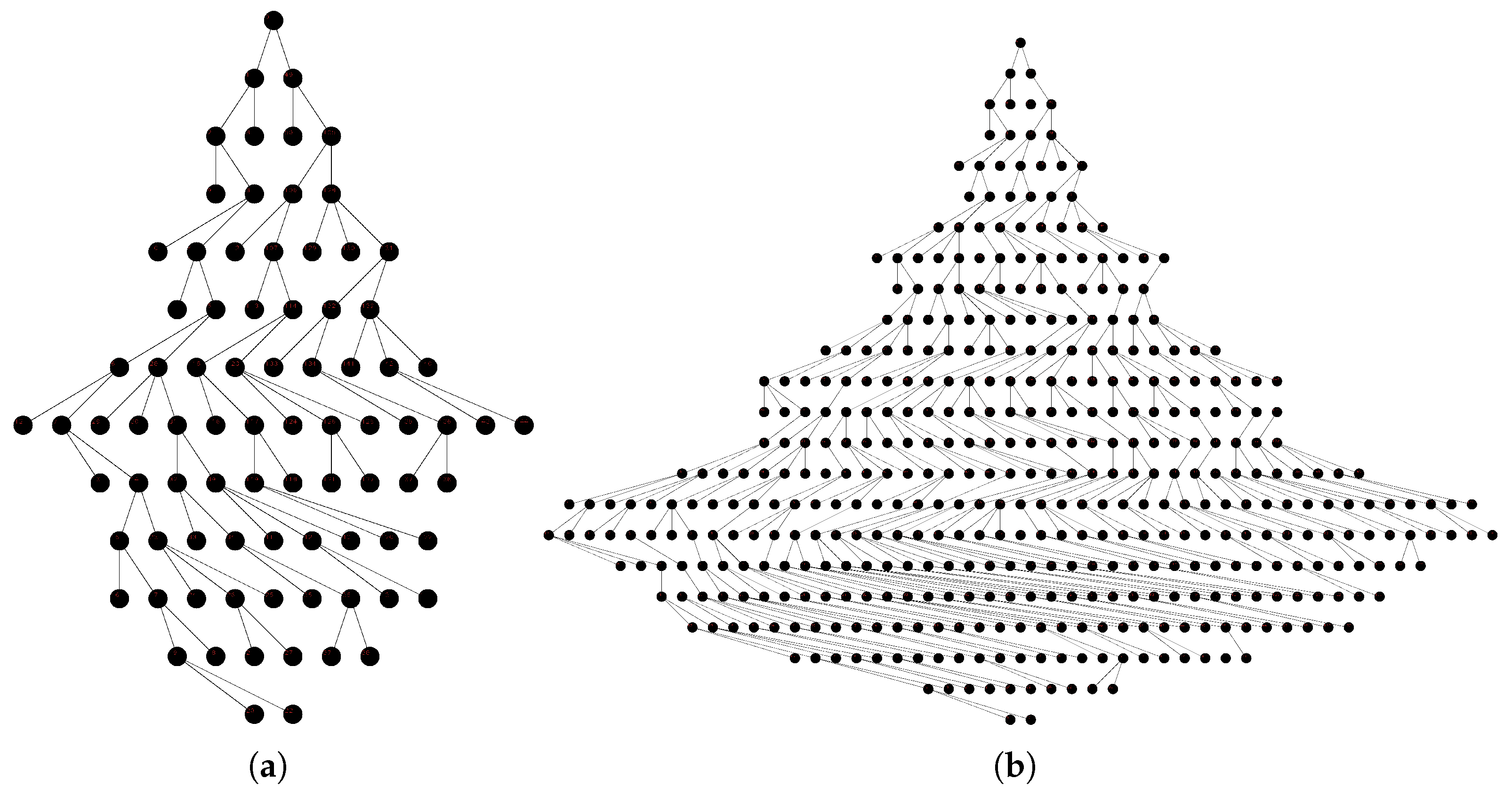
Now we consider the consequence of applying Algorithm 2 to our example. First of all, the number of nodes dramatically increases, because in this case each cyclic return during Algorithm 2 approximately doubles the number of cycles for future returns. That is, if we let each cycle repeat two times, we get $\overline{n}=91+4\times (14\times 4)+2\times ((14+2)\times 4)=91+2^2\times 56+2^1\times 64$. Here we get 91 by adding 8 cycle nodes to 83 initial nodes, the total number of nodes in all cycles is equal to 56 and we add 8 (resulting in 64) cycle nodes for all extension iterations except for the last one. In the general case (with any maximum depth), we can calculate the number of nodes with the formula

$$\overline{n}\left(m\right)=\left\{\begin{array}{cc}91+56·2^m+{\displaystyle \sum _{i=1}^{m-1}}64·2^i=\mathcal{O}\left(2^m\right),\hfill & m\ge 1\\ 83,\hfill & m=0\end{array}\right.,$$

(5)

where m is the maximum number of repeats for cycles, that is, with a large m the number of nodes doubles as m increases by 1. However, as we already mentioned before, m is small in the considered case, and therefore, this technique is suitable. The graphical illustrations for a graph without cycles and with cycles, and $m=2$, are presented in Figure 4.

Next, we apply Algorithms 3–5 to obtain the profit distribution that is provided in

Table 4. The profit distribution.

X	−4831.46	−2794.58	−417.96	3329.63	3389.63	3439.63	3489.63
P(X)	0.0000305	0.0000770	0.0002775	0.06	0.00227966	0.00593781	0.931398

.

As we see from Table 4, only seven different values can occur. Negative values represent project failures, however, some of them are considerably smaller than others; for example, we see that with probability 0.0002775, the profit is $-417.96$, which is not as bad as the value of $-4831.46$. This difference is caused by different time intervals before the failure occurs, that is, in the beginning of the project the costs spent on the building process are small. Thus, this information can be very important for risk management. The project profit expected value is equal to 3477.68, however, it is not informative for risk evaluation. The decisions that were made in decision nodes are stored in a graph—the chosen edges have probabilities equal to 1, and the remaining ones have probabilities equal to 0. In total, 63 decisions were made by the program. Since we have no notations for the subtree from node $C_8^a$ (as well as all nodes that were generated by the cycle-expansion algorithm), and some decisions are different than in the subtree from node $C_1$, we do not provide the set of decisions; we consider this as non-informative in the current research.

We see some negative values in Table 4, which means that in the considered case, the expected profit value is bigger in the case of the law violation. That is, small probabilities of getting negative incomes lower the expected profit by a smaller value than the possible project modification does (i.e., building according to an alternative project without the law violations). It is an open question whether such violation makes a negative impact on sustainability of city development. However, the bigger profit for construction investors can be followed by further investments resulting in a more sustainable city growth. The more detailed study of advantages and disadvantages of such a case in terms of sustainable city development is out of the scope of this research. Such a study would rely on more detailed information about violations, which can be found in other papers for Lithuanian cases [17].

We note that in the general case, after cyclic repeats of events, the decisions can become different. This means that if we did not expand these cycles, the strategies would be selected (by some means) and fixed—which could be not optimal. On the other hand, the number of cycles could be unlimited, for example, if we apply some implementation of a Monte Carlo method. However, as was mentioned before, it is reasonable to limit the number of cyclic repeats due to specificity of the real process (the initial assumption of unlimited repeats of events with constant probabilities, and its usage in a graph, is quite artificial). Thus, we conclude that our proposed algorithm fits the considered problem very well.

5. Conclusions

In this paper, the real-life example of the process of judicial conflict resolution was considered. It was found that the time estimation is important when the costs of failures strongly depend on time. It is obvious that in the considered case, the failure at the beginning stages of building construction is much less costly than the failure at the later construction stages. Thus, for modelling of the impact of such judicial processes on investment, the evaluation of time is critical. The proposed approach allows us to evaluate the project with an estimation of time. Identifying big risks is important to avoid project failures, and it also lets investors select the appropriate projects for investment.

It is normal for judicial processes to return back to the previous stages (e.g., a court of appeal returns to a court of first-instance), increasing the time of the judicial process, and therefore, it is important to evaluate such cyclic event repeats. However, in practice, the number of repeats for such events is limited, and therefore, we used that idea directly in the proposed cyclic-expansion algorithm to convert a graph into a tree by limiting the number of cyclic event repeats. Firstly, we apply the cyclic-expansion algorithm. Secondly, we apply the algorithm to calculate the parameters for end nodes by recursively accumulating time and costs through a tree (using pre-order tree traversal). Thirdly, we use an algorithm that is based on a post-order tree-traversal idea to evaluate all nodes and select the optimal strategy. Thereafter, the simple pre-order tree-traversal algorithm is applied to accumulate the probabilities and compute the distribution of scenario values.

In the general case, after cyclic repeats of events, the decisions can become different. Thus, the tree expansion is important, because it allows repeated decision nodes to have different values. The initial assumption of unlimited repeats of events with constant probabilities, and its usage in a graph, is quite artificial. Thus, it is optimal to limit the number of cyclic repeats due to specificity of the real process; this leads to the proposed cyclic-expansion approach directly.

After extracting the profit distribution of the project, it is impossible to estimate the project uniquely—it strongly depends on investors’ demands (i.e., risk versus profit evaluation). The analysis of the risk evaluation from the profit distribution is out of the scope of this research, and therefore, we consider the profit distribution as a final result of application of the proposed algorithm.

It is important to note that the algorithm does not identify the importance of the law violations in terms of sustainability. However, it could indicate in which cases the law violations are profitable for construction investors, that is, which cases need an additional investigation. In practice, it can be used in two ways. (1) By investors in a decision-support system to avoid risks of conflicts with society. (2) By institutions that control the development of territorial-planning procedures to identify and eliminate the weakness in law and regulations systems. If such kinds of tools were used in both suggested cases simultaneously, this would greatly contribute to a sustainable city development, because it would lead to much more predictable and sustainable behaviour of construction-process participants. In a similar way, the algorithm can be used by a scientific community to model how changes of territorial-planning procedures and laws impact the behaviour of construction-process participants. Thus, the proposed algorithm can support the development of rules regulating the construction process.

References

- Davidov, S.; Pantoš, M. Stochastic assessment of investment efficiency in a power system. Energy 2017, 119, 1047–1056. [Google Scholar] [CrossRef]
- Li, C. Empirical Study on the Impact Factors of the Investment Efficiency of Urbanization Construction in Guizhou Province, China. DEStech Trans. Econ. Manag. 2016. [Google Scholar] [CrossRef]
- Focacci, A. Managing project investments irreversibility by accounting relations. Int. J. Proj. Manag. 2017, 35, 955–963. [Google Scholar] [CrossRef]
- Shariatmadari, M.; Nahavandi, N.; Zegordi, S.H.; Sobhiyah, M.H. Integrated resource management for simultaneous project selection and scheduling. Comput. Ind. Eng. 2017, 109, 39–47. [Google Scholar] [CrossRef]
- Marugán, A.P.; Márquez, F.P.G.; Lev, B. Optimal decision-making via binary decision diagrams for investments under a risky environment. Int. J. Prod. Res. 2017, 55, 5271–5286. [Google Scholar] [CrossRef]
- Zavadskas, E.K.; Turskis, Z.; Antucheviciene, J. Selecting a contractor by using a novel method for multiple attribute analysis: Weighted Aggregated Sum Product Assessment with grey values (WASPAS-G). Stud. Inform. Control 2015, 24, 141–150. [Google Scholar] [CrossRef]
- Trinkūnienė, E.; Podvezko, V.; Zavadskas, E.K.; Jokšienė, I.; Vinogradova, I.; Trinkūnas, V. Evaluation of quality assurance in contractor contracts by multi-attribute decision-making methods. Econ. Res. Ekon. Istraž. 2017, 30, 1152–1180. [Google Scholar] [CrossRef]
- Lazauskas, M.; Kutut, V.; Zavadskas, E.K. Multicriteria assessment of unfinished construction projects. Gradevinar 2015, 67, 319–328. [Google Scholar]
- Suh, S.; Suh, W.; Kim, J.I. Risk analysis model for regional railroad investment. Eng. Comput. 2017, 34, 164–173. [Google Scholar] [CrossRef]
- Xu, J.; Zhao, S. Noncooperative Game-Based Equilibrium Strategy to Address the Conflict between a Construction Company and Selected Suppliers. J. Constr. Eng. Manag. 2017, 143, 04017051. [Google Scholar] [CrossRef]
- Bellman, R. A Markovian Decision Process. Indiana Univ. Math. J. 1957, 6, 679–684. [Google Scholar] [CrossRef]
- Richey, M. The evolution of Markov chain Monte Carlo methods. Am. Math. Mon. 2010, 117, 383–413. [Google Scholar] [CrossRef]
- Šostak, O.R.; Vakrinienė, S. Mathematical modelling of dispute proceedings between investors and third parties on allegedly violated third-party rights. J. Civ. Eng. Manag. 2011, 17, 126–136. [Google Scholar] [CrossRef]
- Šostak, O.R. Planning Development of Construction by Taking Into Account Interests of the Third Parties (Doctoral Dissertation, in Lithuanian). Ph.D. Thesis, Vilnius Gediminas Technical University, Vilnius, Lithuania, 2011. [Google Scholar]
- Celik, T.; Kamali, S.; Arayici, Y. Social cost in construction projects. Environ. Impact Assess. Rev. 2017, 64, 77–86. [Google Scholar] [CrossRef]
- Mitkus, S.; Šostak, O.R. Modelling the process for defence of third party rights infringed while implementing construction investment projects. Technol. Econ. Dev. Econ. 2008, 14, 208–223. [Google Scholar] [CrossRef]
- Mitkus, S.; Šostak, O.R. Preservation of healthy and harmonious residential and work environment during urban development. Int. J. Strateg. Prop. Manag. 2009, 13, 339–357. [Google Scholar] [CrossRef]
- Šostak, O.R.; Makutėnienė, D. Timely determining and preventing conflict situations between investors and third parties: Some observations from Lithuania. Int. J. Strateg. Prop. Manag. 2013, 17, 390–404. [Google Scholar] [CrossRef]
- Šostak, O.R.; Makutėnienė, D. Modelling a dispute hearing between an investor and the public concerned in administrative courts of the republic of Lithuania. Technol. Econ. Dev. Econ. 2013, 19, 489–509. [Google Scholar] [CrossRef]
- Zhou, W.Z.; Peng, Y.; Bao, H.J. Regular pattern of judicial decision on land acquisition and resettlement: An investigation on Zhejiang’s 901 administrative litigation cases. Habitat Int. 2017, 63, 79–88. [Google Scholar] [CrossRef]
- Manasse, P.; Savona, R.; Vezzoli, M. Danger Zones for Banking Crises in Emerging Markets. Int. J. Financ. Econ. 2016, 21, 360–381. [Google Scholar]
- Stević, Ž.; Pamućar, D.; Vasiljević, M.; Stojić, G.; Korica, S. Novel Integrated Multi-Criteria Model for Supplier Selection: Case Study Construction Company. Symmetry 2017, 9, 279. [Google Scholar] [CrossRef]
- Santos, S.F.; Fitiwi, D.Z.; Bizuayehu, A.W.; Shafie-Khah, M.; Asensio, M.; Contreras, J.; Cabrita, C.M.P.; Catalão, J.P.S. Impacts of Operational Variability and Uncertainty on Distributed Generation Investment Planning: A Comprehensive Sensitivity Analysis. IEEE Trans. Sustain. Energy 2017, 8, 855–869. [Google Scholar] [CrossRef]
- Eisenhardt, K.M. Agency theory: An assessment and review. Acad. Manag. Rev. 1989, 14, 57–74. [Google Scholar]
- Mitroff, I.I. Stakeholders of the Organizational Mind; Jossey-Bass: San Francisco, CA, USA, 1983. [Google Scholar]
- Gras-Gil, E.; Manzano, M.P.; Fernandez, J.H. Investigating the relationship between corporate social responsibility and earnings management: Evidence from Spain. Brq-Bus. Res. Q. 2016, 19, 289–299. [Google Scholar] [CrossRef]
- Martinez-Ferrero, J.; Gallego-Alvarez, I.; Garcia-Sanchez, I.M. A Bidirectional Analysis of Earnings Management and Corporate Social Responsibility: The Moderating Effect of Stakeholder and Investor Protection. Aust. Account. Rev. 2015, 25, 359–371. [Google Scholar] [CrossRef]
- Schwarzmüller, T.; Brosi, P.; Stelkens, V.; Spörrle, M.; Welpe, I.M. Investors’ reactions to companies’ stakeholder management: the crucial role of assumed costs and perceived sustainability. Bus. Res. 2017, 10, 79–96. [Google Scholar] [CrossRef]
- GooGle. Object Location on GooGle Maps. 2017. Available online: https://www.google.lt/maps/place/%C5%A0e%C5%A1kin%C4%97s+g.+45C,+Vilnius+07158/@54.7184175,25.2479231,17z/data=!4m5!3m4!1s0x46dd915d44d79665:0x5a00399e0ea3ff3b!8m2!3d54.7184175!4d25.2501118?hl=en (accessed on 11 January 2018).
- Lithuanian State Enterprise Centre of Registers. On the Data About the Real Estate; Document Number (7.2./1147)s-1689; Lithuania, 2007. Available online: http://techmat.vgtu.lt/~ab/docs/EnterpriseRegisters.pdf (accessed on 11 January 2018). (In Lithuanian).
- Www.inreal.lt. Real Estate Market Overview for 2007 Year. 2008. Available online: http://www.inreal.lt/media/editor/inreal/rinkos-apzvalgos/2007_metine_apzvalga.pdf (accessed on 11 January 2018). (In Lithuanian).
- Vilnius County Head Administration. The Copy of the Act of Building Usage Suitability. Document Number (100)11.55-134. Lithuania, 2007. Available online: http://techmat.vgtu.lt/~ab/docs/HeadAdministrationDoc.pdf (accessed on 11 January 2018). (In Lithuanian).
- 690th Dwelling House Construction Association, (Lithuania, Company Code 125112766). Reference Number 20: About Funds Used for Object Financing. 2005. Available online: http://techmat.vgtu.lt/~ab/docs/Bendrija.jpg (accessed on 11 January 2018). (In Lithuanian).
- Weng, S.S.; Yang, M.H.; Koo, T.L.; Hsiao, P.I. Modeling the prediction of business intelligence system effectiveness. SpringerPlus 2016, 5, 737. [Google Scholar] [CrossRef] [PubMed]
- Bellman, R.E.; Dreyfus, S.E. Applied Dynamic Programming; Princeton University Press: Princeton, NJ, USA, 2015. [Google Scholar]
Figure 1.
The graph for the considered example. copies the node and all nodes following from it.
Figure 2.
Average daily costs.
Figure 3.
The relations between a node and its parent and child nodes.
Figure 4.
The impact of the Algorithm 2 on graph. (a) The graph without cycles, , ; (b) the graph with ().