Groundwater Level Dynamics in Bengaluru City, India
by
 ,
,
M. Sekhar
1, 
Sat Kumar Tomer
2,
S. Thiyaku
2,
P. Giriraj
1,
Sanjeeva Murthy
1 and
Vishal K. Mehta
3,* 1
Department of Civil Engineering and Indo-French Cell for Water Sciences, Indian Institute of Science, Bangalore 560012, India
2
Aapah Innovations, Gachibowli 500032, Hyderabad, Telangana 50003, India
3
Stockholm Environment Institute, 400 F St, Davis, CA 95616, USA
*
Author to whom correspondence should be addressed.
Sustainability 2018, 10(1), 26; https://doi.org/10.3390/su10010026
Submission received: 17 November 2017
/
Revised: 18 December 2017
/
Accepted: 19 December 2017
/
Published: 22 December 2017
(This article belongs to the Special Issue Sustainability in an Urbanizing World: The Role of People)
Abstract
:Groundwater accounts for half of Indian urban water use. However, little is known about its sustainability, because of inadequate monitoring and evaluation. We deployed a dense monitoring network in 154 locations in Bengaluru, India between 2015 and 2017. Groundwater levels collected at these locations were analyzed to understand the behavior of the city’s groundwater system. At a local scale, groundwater behavior is non-classical, with valleys showing deeper groundwater than ridge-tops. We hypothesize that this is due to relatively less pumping compared to artificial recharge from leaking pipes and wastewater in the higher, city core areas, than in the rapidly growing, lower peripheral areas, where the converse is true. In the drought year of 2016, groundwater depletion was estimated at 27 mm, or 19 Mm3 over the study area. The data show that rainfall has the potential to replenish the aquifer. High rainfall during August–September 2017 led to a mean recharge of 67 mm, or 47 Mm3 for the study area. A rainfall recharge factor of 13.5% was estimated from the data for 2016. Sustainable groundwater management in Bengaluru must account for substantial spatial socio-hydrological heterogeneity. Continuous monitoring at high spatial density will be needed to inform evidence-based policy.
1. Introduction
Groundwater is an important, decentralized source of drinking water for millions of people in India. It meets nearly 85% of rural domestic water needs and 50% of urban water needs [1]. Dependence on groundwater for water-supply in urban towns and cities is increasing due to accelerated growth, increasing per capita water use and poor reliability of imported surface water from distant sources [2,3]. In a review of urban recharge, Lerner [4] describes how urbanization affects the groundwater cycle by way of changes to both the total water budget, and to pathways recharge. The total imported water supply of many temperate European cities is comparable to the annual rainfall endowment, while, in many dense cities in arid areas, water supply imports are greater than annual rainfall. Leakage through water supply pipes then becomes a major source of recharge. In cities with inadequate sewerage systems, leakage through septic tanks and soakpits, and untreated wastewater released into drainage channels, are also major components of recharge quality. While these anthropogenic flows increase groundwater recharge, natural recharge rainfall can decrease in dense built-up areas of towns and cities, where a significant proportion of land surface is altered through soil compaction, roofing and paving, all of which reduce normal infiltration. The net effect on the groundwater budget also depends on the level of pumping from the aquifer. Spatio-temporal variation in the anthropogenic components and spatial variation hydrogeological properties such as specific yield and transmissivity add to the complexity of urban groundwater systems. Thus, reflecting the diversity of development pathways, geographies and geohydrology, urbanization induced changes to the groundwater system may include sharp changes of groundwater levels [5,6,7]; reduced well yields and deterioration in quality of groundwater [5,8,9,10]; poor quality base flow [1]; and migration of polluted urban groundwater into surrounding areas [11,12].
In rapidly growing Indian cities, both imported surface water and groundwater pumping have been increasing apace [13]. At the same time, sewer line connections, and wastewater treatment in Indian cities are severely lacking, with the Government of India acknowledging that some 70% of wastewater is estimated to be released without treatment into drainage features [14]. Increased recharge from anthropogenic sources (leaking water supply and wastewater systems), and increased pumping from the aquifer are likely to be occurring simultaneously. One of the goals of groundwater management plans in such circumstances is to safeguard groundwater levels in urban aquifers by influencing the magnitude and use of groundwater pumping. This requires a scientific understanding of urban groundwater systems based on a comprehensive database of groundwater levels, availability and use at appropriate spatial scale. Depending upon the groundwater monitoring network, spatial variations of recharge and of hydrogeological properties such as specific yield can also be estimated (e.g., [15]). Such monitoring is essential to help inform hydrogeological models that could be used for support towards sustainable urban groundwater management.
However, the majority of studies utilizing simple to complex groundwater models have been in large agricultural catchments (e.g., [4,16]). Investigations of urban groundwater systems, especially in developing countries, are limited [10,17,18,19,20,21]. In India, only two comprehensive urban groundwater studies have combined monitoring with models. Sekhar and Kumar [22] monitored 472 wells to study and model the groundwater dynamics of a central, 27 km2 portion of Bengaluru, to assess the possible groundwater impacts related to the underground section of the city’s metro rail system. A second study comprehensively evaluated groundwater for the small city of Mulbagal, 95 km from Bengaluru [21]. Groundwater levels in 272 wells covering 50 km2 were monitored for three years. A distributed groundwater model was built based on this dataset, and applied to investigate climate and demographic scenarios for the city. These investigations highlight the fact that models can be built only if there is an adequate spatial representation of the groundwater monitoring network. In India, the nationwide long-term groundwater level monitoring by the Central Groundwater Monitoring Board (CGWB) is on average at a density of one station for approximately every 100 km2. This density is very coarse if one wants to model urban systems, which usually cover areas of a few tens to few hundreds of square kilometers. Heterogeneous characteristics (e.g., hydraulic conductivity, transmissivity, and specific yield) of the aquifer in hard rock areas that underlie much of peninsular India add another good reason for a dense network of wells for small scale urban systems.
In this paper, we focus on understanding the groundwater patterns and dynamics in Bengaluru (earlier known as Bangalore), India. Bengaluru is one of the fastest growing cities in Asia, where population has grown from 180,366 in 1891 [23] to 8.5 million in 2011 [24]. The area of city limits, as by the municipal boundaries, has also grown substantially—ten times from a mere 75 km2 in 1901 [25]. Water supply from the utility, Bengaluru Water Supply and Sewerage Board (BWSSB) has grown, but not managed to keep up with the rapid growth in demand. The inability of utility water supply growth to keep up with the city’s growth is well documented (e.g., [24,26]). As a result, similar to all Indian cities, groundwater is heavily used to make up the deficit. Although based on a sparse monitoring network, the CGWB has estimated that groundwater is more than 100% developed in Bengaluru, which means that abstraction (pumping) is more than recharge to the aquifer [25]. In this paper, we report on the establishment of an innovative, dense monitoring network across the city, with the objectives of: (i) collecting a time series of groundwater table depths and using the data to study the spatial patterns in groundwater levels; (ii) estimating net groundwater storage changes during drought year 2016 and during extreme rainfall periods; and (iii) estimating the rainfall recharge factor net groundwater flux. Our intention in this paper is to describe the patterns observed and to estimate the net groundwater storage change and aggregate flows, based on the water table method. In the Conclusions Section, we describe a more elaborate modeling framework that will be used in a forthcoming paper to estimate separate components of the groundwater budget.
2. Materials and Methods
2.1. Study Area
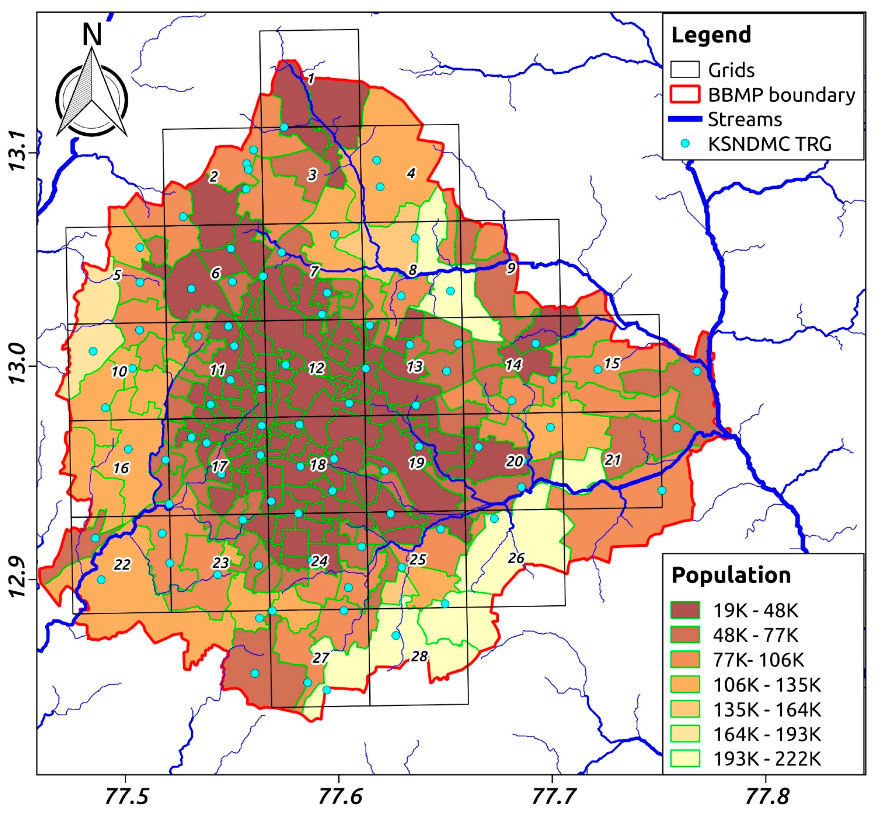
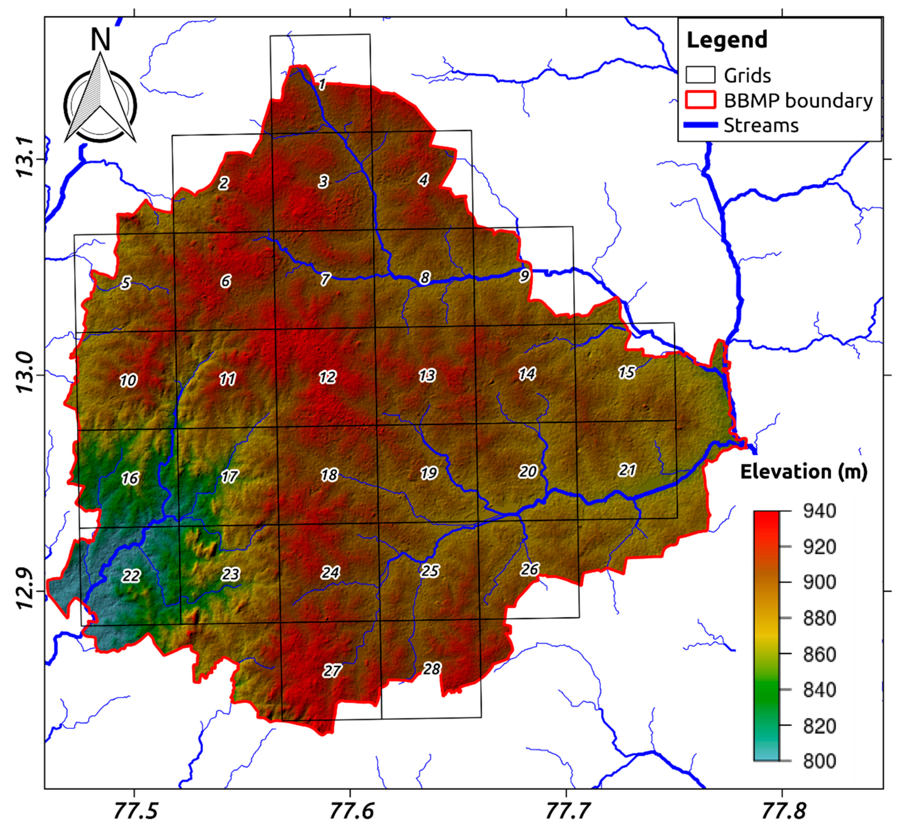
Bengaluru city is situated within 12°45′N–13°10′N and 77°25′E–77°45′E, and covers an area of 720 km2 (Figure 1). The city core is at 900 to 930 m amsl (above mean sea level), on a divide with a roughly North–South axis, with the Arkavathi River drainage Westward to the River Cauvery, and the South Pennar drainage to the East (Figure 2) [24]. The climate is semiarid with normal rainfall of 820 mm, September being the peak rainfall month. Close to 60% of the rainfall on average occurs during the southwest monsoon from June to September [27]. The retreating, northeast monsoon also brings rain from October to December. The dry period extends from January to May, although convectional thunderstorms occur from March through May. Typically, January and February receive almost no rain.
Except for a few central areas in the old city core, the population growth between 2001 and 2011 has been positive with some outer areas reaching a growth of more than 300% [26]. The water needs of the city are mainly met by surface water supply from Cauvery River, and from groundwater. Surface water imported from the Cauvery River, currently at close to 1400 million liters per day (MLD), is approximately 75% of the average rainfall over the city, signaling the substantial anthropogenic influence on the urban water budget [26]. Non-revenue water, made up largely of leakage losses, was almost 50% in 2011 [24]. Although surface water supply has increased over time, it has been unable to catch up with the rapid growth and expansion of the city [26]. As a result, groundwater provides a large proportion of the current water consumption, and is likely to continue to do so in several wards of the municipality, which is called called Bruhath Bengaluru Mahanagara Palike (BBMP) (see Figure 3). There is no effective regulation of the use of groundwater in these wards for domestic, commercial, industrial or government agency purposes. Free and unrestricted use is made of this resource by households, businesses, institutions and government agencies, including the Bengaluru Water Supply and Sewerage board (BWSSB). Consequently, there is practically no reliable data on the rate and distribution of groundwater withdrawals. Monitoring of the aquifers from which groundwater is withdrawn is conducted by the Department of Mines and Geology (DMG) and the Central Ground Water Board (CGWB). Both these organizations conduct regional exploration and investigation programs. Although many wells are used for pumping groundwater in the city, the density of the existing monitoring networks is very low [27]. Furthermore, the temporal frequency of monitoring by CGWB is once every few months. Hence, even though this dataset might reveal some larger, regional scale groundwater behavior over many years, it is not useful for assessing the state of the urban groundwater system; its resilience to important stressors such as anthropogenic forcings and drought conditions; and its response to extreme rain events.
2.2. Groundwater Monitoring
The first step was to create a comprehensive database for the city. Groundwater table mapping was carried out between December 2015 and September 2017. Groundwater levels (GWL) were measured using a monitoring network of 158 wells in an area of 700 km2. Out of these 158 wells, 154 wells had an unbroken record through the study period and were selected for the analysis reported here. The monitoring network was established using a novel approach in which the existing wells (predominantly municipal bore wells) were used as piezometers where groundwater levels were measured. To achieve a uniform spatial distribution, the study area was divided into grids of 5 km × 5 km, resulting in 28 grids for the city. Monitoring wells should be free from pumping to be used as piezometers. Those municipal wells that were not in use were carefully selected in each grid. In each grid, 5–6 monitoring wells were established. Groundwater levels were measured each month using a manual water level sensor (Heron Instruments Inc.). Figure 4 shows the location of the 154 groundwater monitoring locations, along with land-cover. The inner part of the city has relatively higher built-up area. Several secondary datasets, assembled at the grid scale, are presented in Table 1.
Maps were interpolated from the depth to GWL measurements using ordinary kriging. Kriging has been found to perform better than inverse distance weighting [28,29], and has been used in other studies in hard-rock aquifers in southern India [15,21,22,30]. Kriging was performed using the geoR library of R (https://cran.r-project.org/package=geoR). Variograms for each month were fitted using numerical optimization. Exponential variograms were found to fit the data well, and used to create interpolated maps of depth to groundwater (DGW) at a spatial grid of 100 m.
2.3. Rainfall Data
Annual rainfall for more than 100 years (1901–2012) is shown in Figure 5. During this period, the maximum, minimum and average annual rainfall were 1527, 393 and 880 mm, respectively. Daily rainfall data covering the study period were collected from about 150 stations maintained by the Karnataka State Natural Disaster Monitoring Cell (KSNDMC) for the period January 2015–October 2017. The spatial distribution of these KSNDMC rainfall gauges is shown in Figure 1. A plot of monthly rainfall averaged over these stations is shown in Figure 6. Total rainfall (January–December) for the years 2015, 2016 and 2017 (up to October 2017) was 1153, 716 and 1435 mm. The intra-year rainfall distribution during these three years has strong variability, and each year was quite different. In all three years, the southwest monsoon rainfall was much lower than normal. However, during 2015 and 2017, there were extreme rainfall events, while 2016 was a drought year. In 2015, the months of September–November produced about 50% of the annual rainfall. In 2016, the months of May–July produced about 70% of the annual rainfall. In 2017, the months of August–October produced about 75% of the annual rainfall. The 2017 rainfall was close to the highest received rainfall in more than 100 years. These patterns of drought conditions and extreme rain events over the study period provided a natural opportunity to study the response and resilience of Bengaluru’s groundwater system.
2.4. Cluster Analysis
In order to aid the interpretation of observed groundwater patterns, a clustering analysis was performed using the secondary data in Table 1. Hierarchical cluster analysis was applied to explore the number of distinct clusters emerging from the secondary data. Ward’s linkage algorithm is used for hierarchical clustering by minimizing the increase in total within-cluster sum of squared error [32]. The optimal number of clusters were identified by visual inspection of the resulting dendrogram.
2.5. Groundwater Analysis
The Water Table Fluctuation (WTF) method was used to estimate the storage change, natural recharge and net outflow for distinct periods of observation. The advantage of the WTF method, described comprehensively in Healy and Cook [33], is that it is a simple method that relies on dense groundwater level measurements, has only one parameter (the specific yield), and no assumptions are made on the mechanisms by which water recharges the aquifer. The WTF method is used in India for operational annual groundwater recharge assessment by government agencies [34]. Nationally, it is performed by delineating the land area into watersheds or catchments with an area of about 600–1000 km2. This scale is tied to the density of long term observation network which is approximately one observation well per 100 km2. Recharge assessment for a year is performed for each of these catchments, treating them as one unit or cell. Several researchers have used variations of the WTF method in southern Indian hard-rock aquifers [15,21,22,35]. We use WTF in two ways in this paper, described below.
2.5.1. Natural Recharge and Net Outflow
First, we use the “double water table fluctuation method” [15], which involves splitting the groundwater budget into two distinct periods—dry and wet. These authors used the double WTF method in combination with water balance models and detailed information on several water balance components in a 50 km2, unconfined hard rock aquifer research site in southern India, to estimate both recharge and the effective specific yield [15].
In this paper, we apply the double WTF method to estimate rainfall recharge and total net outflow in the same manner as Sekhar et al. [21] did for the town of Mulbagal (mentioned in the Introduction). Because many components of the budget are not known quantitatively for Bengaluru (pumping, and water and wastewater leakage), we use the double WTF to estimate only the rainfall recharge factor (from the wet period), and the net outflow (from the dry period). For the same reason, we cannot independently estimate specific yield as Maréchal et al. [15] did. Instead, we specify specific yield based on the literature and recent experience, and also show the sensitivity of some of our results to this parameter.
The double WTF method is expressed as follows:
where Sy is the specific yield (-), h is the groundwater level (L), t is time (T), R is recharge due to rainfall (LT−1), and Qnet is the net outflow,
where Qout is the total outflow including baseflow, lateral flow and draft. Qin is the recharge to groundwater from anthropogenic flows, i.e., leaking water suppy and wastewater systems (LT−1).
Given the value of Sy and measurements of ∆h, Equation (1) has two unknowns. The equation was written for dry (no or insignificant rainfall) and wet (significant rainfall) periods separately, with the assumption that there was no rainfall recharge during the dry period. After solving both equations, net outflow and rainfall recharge can be computed as,
and
Equation (3) is solved first to estimate the Qnet by applying it over the dry period where ∆tdry is the length of dry period (T). Then, Equation (4) is solved over the wet period where ∆twet is the length of wet period, to estimate R.
2.5.2. Changes in Groundwater Storage
For the net change in groundwater storage in 2016, and from the extreme rainfall months in 2017, the simple form of the WTF is used.
where ∆V is the net storage change (L) and ∆h is the change in groundwater level (L) over a specified period (∆t) (T).
3. Results and Discussion
3.1. Clustering Results
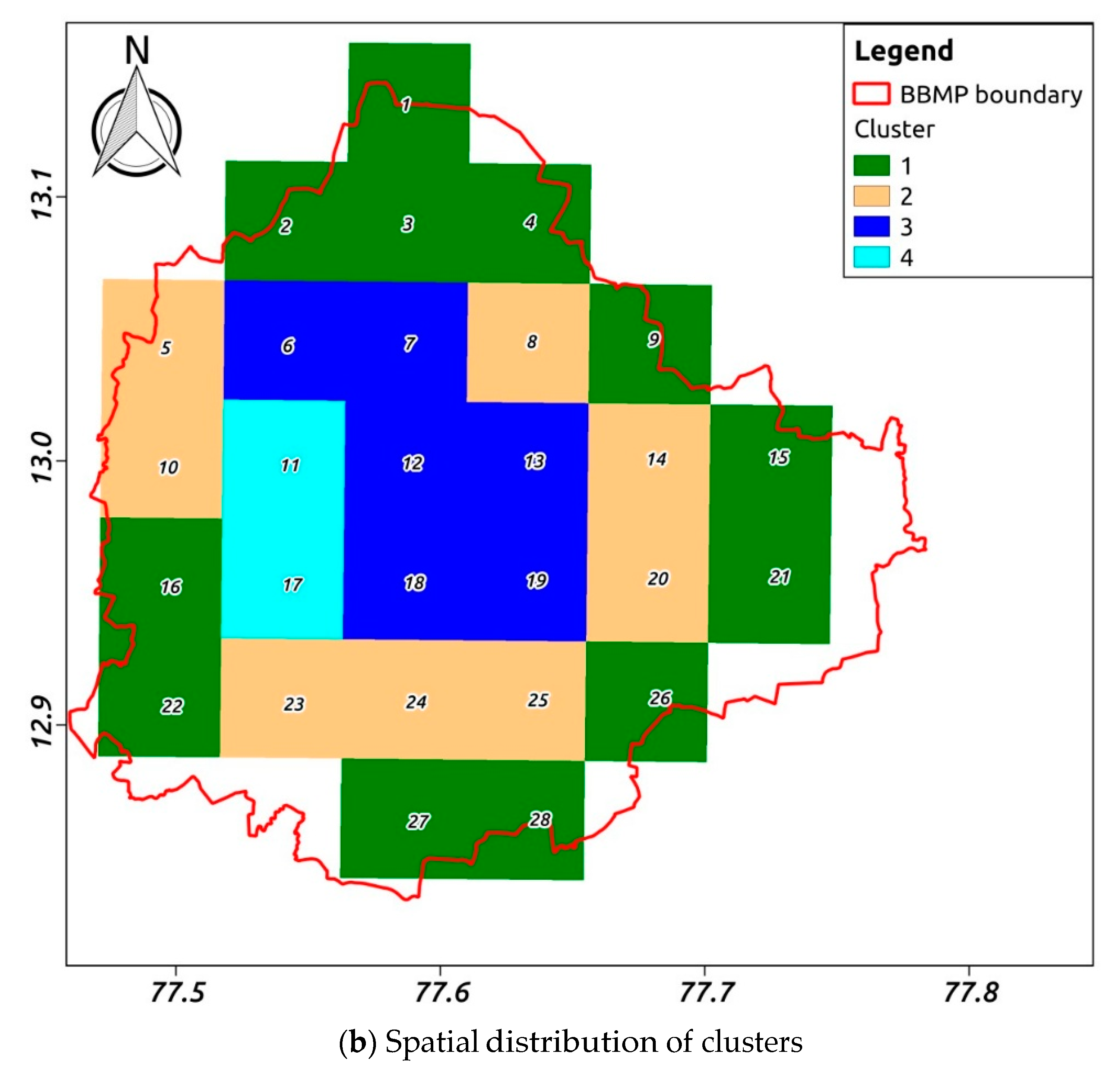
Five variables, as presented in Table 1, were used for the cluster analysis. To account for the location, the distance of each grid from the central grid (#12) was also used in the cluster analysis. Details of the clusters formed are presented in Figure 7 and Table 2. Figure 7a shows the dendrogram obtained from the six variables, which could organize the city into four clusters quite sensibly. The spatial distribution of these four clusters is shown in Figure 7b. Cluster 1 is characterized by the outer periphery, which has significant open space, less water supply from BWSSB and significant groundwater usage. Detailed water supply analysis in [26,36] illustrate that the fast-growing outer areas receive much less water supply than the core areas. Cluster 2 is the inner periphery characterized by moderate groundwater usage, moderate supply of water from BWSSB and moderate open space. Cluster 3 contains grids lying in the central, older parts of the city, which has better water supply from the BWSSB and is densely built-up. Cluster 4 is similar to Cluster 3, except that it has high population density and hence water demand is high and not met by the water supply from BWSSB.
3.2. Groundwater Levels and Dynamics
All groundwater level data collected in various monitoring wells during the period of the study are publicly available (see Supplementary Materials). For the 154 wells over 22 months (December 2015–September 2017), DGW varied from 1 to 72 m, with a mean of 25.74 m and standard deviation of 13.98 m. Figure 8 shows the box and whisker plot of all 154 wells over time. The start in the rise in groundwater level matches with the onset of monsoon season and the shallowest groundwater levels were observed in the peak rainfall month. In 2016, shallowest groundwater is observed in August, while, in 2017, it is observed in September. The groundwater table is deepest in peak summer, in the month of April 2016. It is also deep in April 2017, but the lateness of the 2017 monsoon extended the dry period, resulting in the groundwater table in July 2017 being slightly deeper than that in April 2017. Extremely high rainfall occurred immediately after the dry spell, in August (221 mm) and September (520 mm) 2017. The boxplot shows the groundwater table recovering quite dramatically in response to this extreme rainfall. This extreme rainfall response is investigated further in Section 3.4.
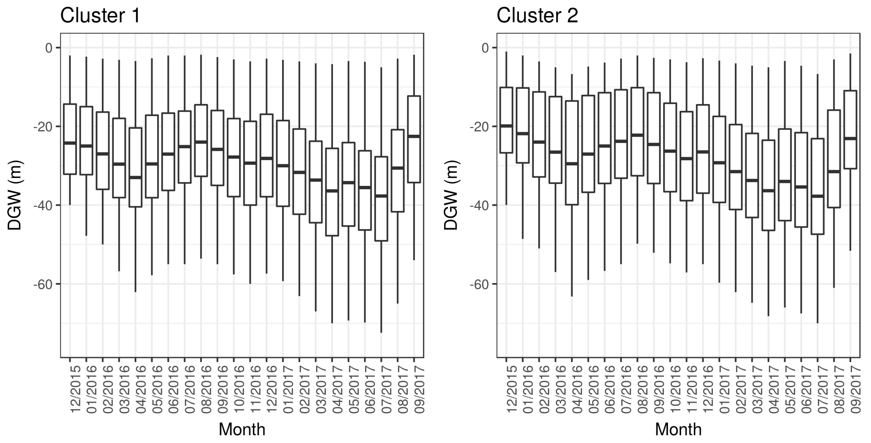
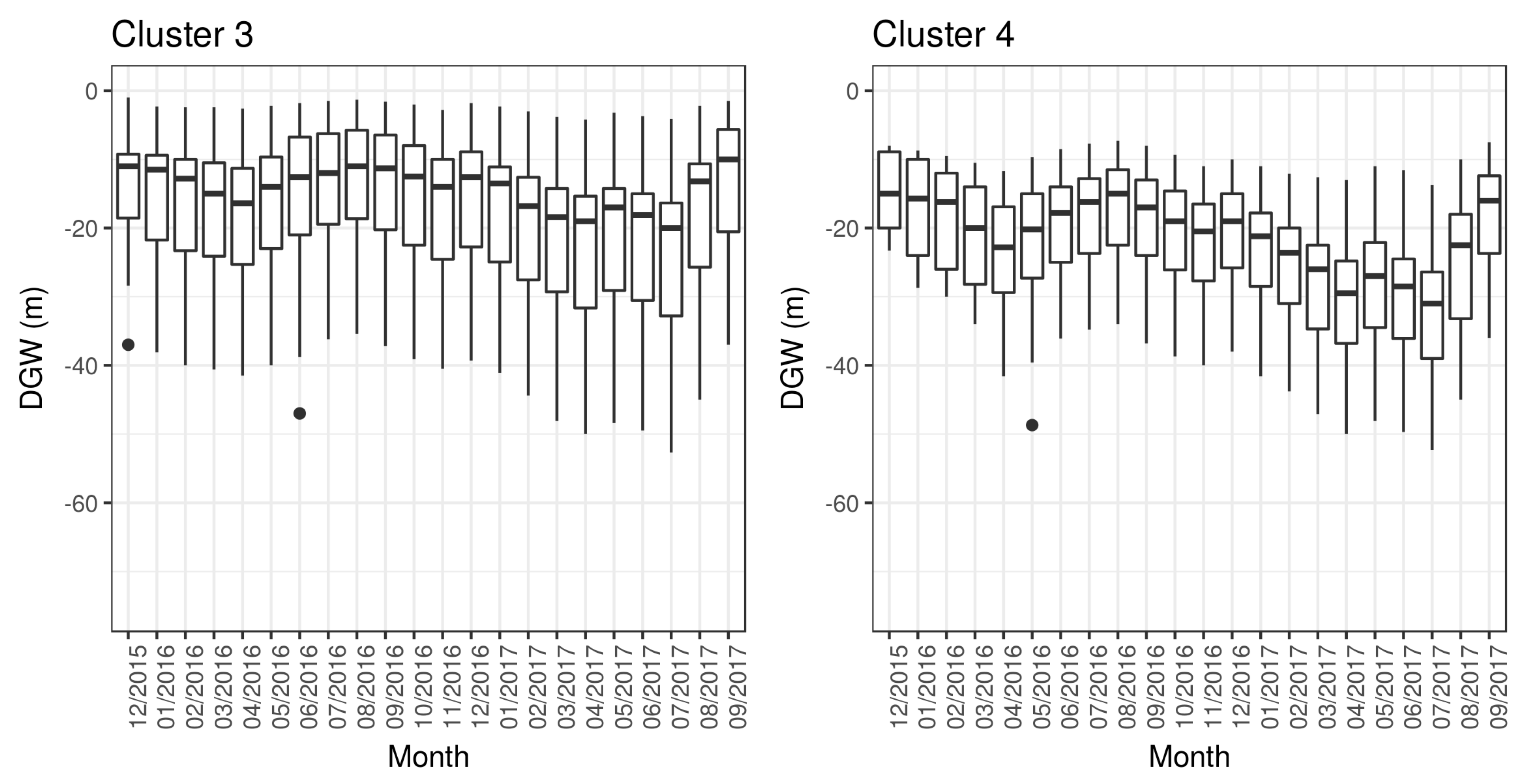
Figure 9 shows the box and whisker plot for 154 wells grouped into the four clusters. Groundwater levels showed substantial spatial and temporal variability in all clusters. A relatively lower variability was observed in Cluster 4 due to less number of grid and data points in this cluster. Mean depths to groundwater table of 29.27 m, 26.22 m, 17.30 m and 23.14 m were observed in Clusters 1–4, respectively. All clusters showed similar temporal variation, as described above. Cluster 3 shows the shallowest groundwater level, which lies in the inner part of the city. This could be due to relatively higher leakage from the sewerage and water supply lines. Cluster 4 showed relatively deeper groundwater level compared to Cluster 3, due to higher water demand (higher population). Cluster 1 showed the deepest groundwater level due to less water supply from BWSSB and high groundwater draft.
Kriged maps of the groundwater table were produced for each month from December 2015 to September 2017. For the monthly variograms used in creating the interpolated maps, the nugget varied from 31.7 m to 127.9 m, partial sill varied from 63.2 m2 to 132.0 m2 and range varied from 1.65 km to 5.44 km. As an example, Figure 10 shows the variograms for two months of 2016. The nugget quantifies the small scale variability present in the data at lag below the average minimum distance among observations. The presence of nugget indicates that a higher small scale spatial variability is present in groundwater level compared to the monitoring network. Studies performed in similar lithology, climate context and scale showed the presence of nugget in an urban catchment (in Mulbagal) [21] and an absence of nugget in agricultural catchments [37]. As suggested by Sekhar et al. [21], the possible reason for the higher small scale variability could be the influence of anthropogenic effects in urban catchments. These variograms suggest that a denser monitoring could be tested in the future, to investigate if, at least in some areas of the city where the nugget is particularly high, an even denser monitoring network is needed. The sill in the variogram indicates the variance in the data. These variograms shows a higher sill when deeper groundwater levels are observed (see Figure 10a) and lower sill when shallowest groundwater levels are observed (see Figure 10b).
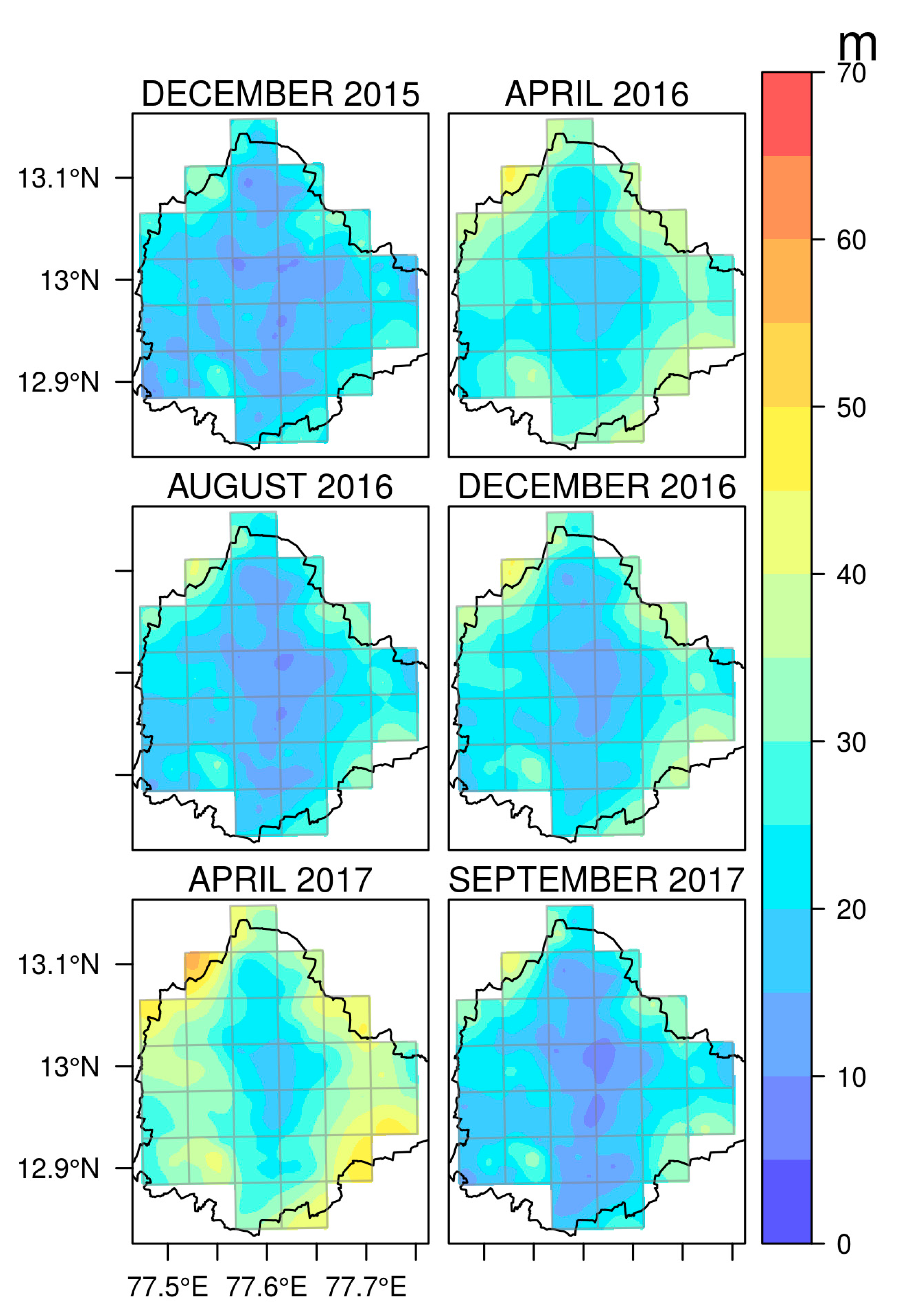
Maps of the groundwater table for a few months are presented in Figure 11. The color legend shown for groundwater level is same across the maps to facilitate comparison. Significant spatial variability in the water levels drawdown and rises are observed in different dry and wet months. Typically, groundwater levels are deeper in April (see DGW for April 2016 in Figure 11) following recession from the previous October (i.e., post-monsoon period). However, in 2017, the deepest groundwater levels in any part of the city were recorded as late as July 2017, because 2016 was a drought year and the monsoon, which typically begins in June, was delayed in 2017.
Most of the grids of Cluster 1 showed relatively deeper groundwater levels, while most of the grids of Cluster 3 showed a relatively shallow groundwater level. The shallow levels in these grids are unaffected even by drought year of 2016 (see April 2016 and July 2016 maps in Figure 11). Shallow groundwater levels in these older, core areas of the city were also observed in a 2009 sampling of 472 wells in central Bengaluru [22]. The secondary data-informed clustering supports the narrative that the shallow groundwater levels in the inner part of the city (Cluster 3) are due to lower groundwater use combined with greater recharge leakage from water and waste water systems in the city. On the contrary, the reason for deeper groundwater levels in the outer areas of the city is due to higher groundwater extraction in the absence of water supply from the water utility agency, the BWSSB. The topography of the city is such that the city center sits at higher elevation, while the newly growing peripheries are at lower elevation. Figure 11 therefore suggests that the lower-lying peripheries have deeper groundwater table than the higher-lying, older city core. This suggests that at a local scale the groundwater behavior is non-classical, i.e., the groundwater is relatively deeper in the valleys than the higher topographic relief. This non-classical behavior of groundwater levels in the valleys points to a deepening of the hydraulic gradient, which could result in greater lateral flows from the city center to periphery areas.
3.3. Rainfall Recharge and Net Outflow
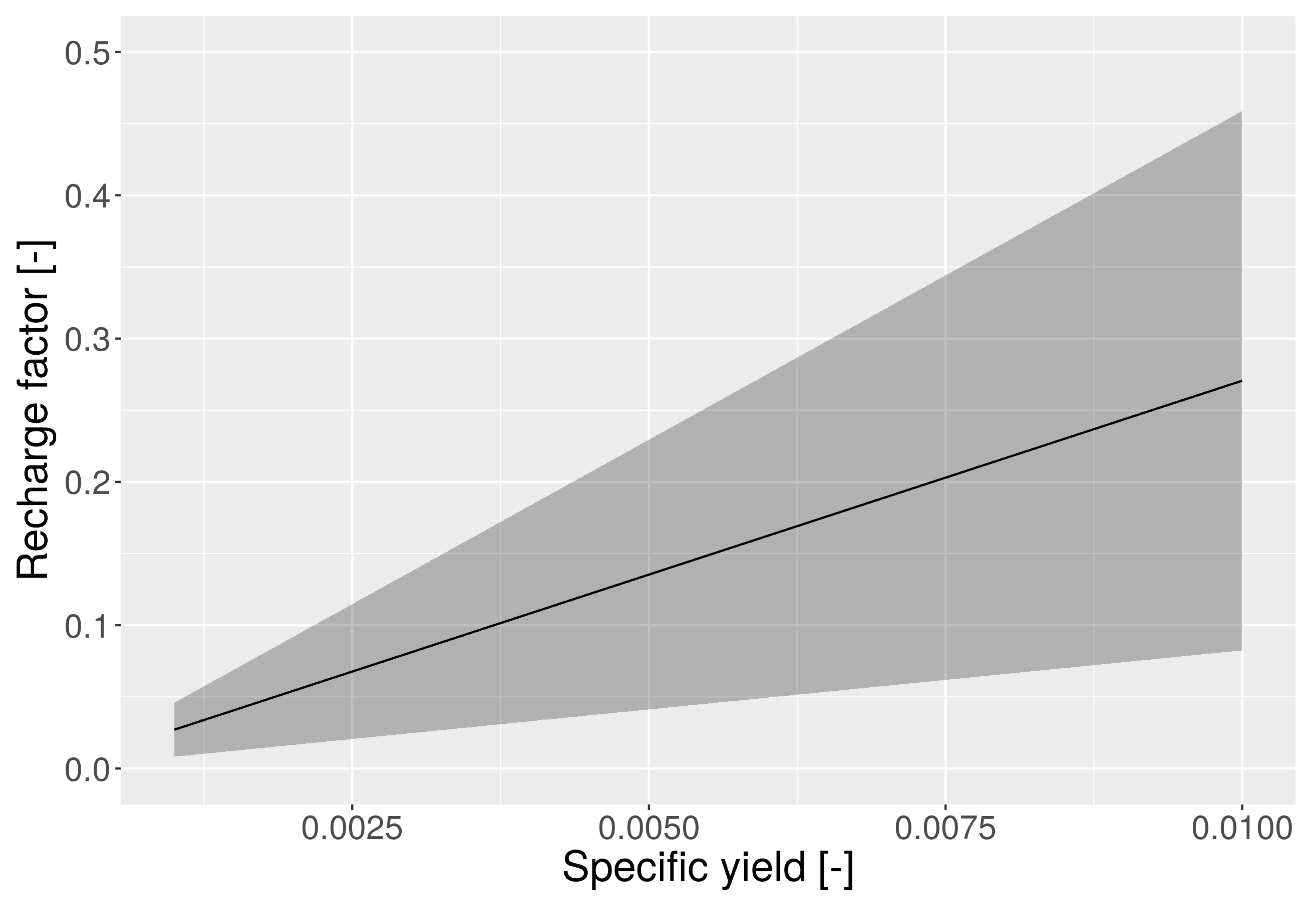
Groundwater balance was estimated using Equations (3) and (4) over 154 monitoring wells. There was insignificant rainfall during January–February (see Figure 6) and it was assumed as dry period. The remaining 10 months (March–December) of 2016 were taken as the wet period. A sensitivity analysis of specific yield to rainfall recharge was performed by varying specific yield from 0.001 to 0.1. The range of specific yield was taken based on the experiments in similar hard rocks (e.g., [21,30]). The natural rainfall recharge factor (annual recharge/annual rainfall) was computed using Equations (3) and (4) for each value of specific yield and is plotted in Figure 12 along with the spatial variability over 154 monitoring wells. The spatial variability in the rainfall recharge factor (RF) increases with the increase in Sy, as expected (refer Equations (4) and (5)). At a Sy of 0.005, the RF is 13.5%, which is close to the range observed in the literature in hard rock, e.g., 15.6% by Maréchal et al. [30], 13–19% by Maréchal et al. [15] and 8.6% by Sekhar et al. [21]. The RF value used by the CGWB for hard rock aquifers is 12% [15]. The RF values used and estimated by these researchers provide a reasonable constraint to the very wide range illustrated in Figure 12. A value of 0.005 was taken as a reasonable assumption of effective specific yield for further analysis.
Using Equation (3), Qnet was estimated to be 123.8 mm with a standard deviation of 82.6 mm and, using Equation (4), R was estimated to be 96.9 mm with a standard deviation of 67.4 mm. The standard deviation was computed over 154 monitoring wells. Table 3 shows the mean and standard deviation of computed Qnet and R over 154 wells for different clusters. Clusters 1 and 2 shows the highest mean values of Qnet and R, and a similar mean value of net storage change. These are periphery areas, with relatively higher open space conducive to more infiltration and rainfall recharge. Cluster 3, covering the core central areas, shows the lowest mean values of Qnet and R. These areas are densely built-up, explaining the low R. One hypothesis for the contrasting behavior of Qnet in central versus periphery areas, as articulated in [25,36] and also suggested by the clustering, is the differential forcings of anthropogenic recharge from leaking water and wastewater versus pumping. In periphery Clusters 1 and 2, Qnet is likely high because of more groundwater use compared to the central Cluster 3, which is better connected to surface water supply.
The difference between the net outflow and recharge listed in Table 3 gives the net change in groundwater storage. As can be seen, in 2016, using the 154 well observations, the net change in groundwater storage is negative in all clusters, i.e., groundwater depletion occurred, as is also apparent in the boxplots presented in Figure 8 and Figure 9. The net storage change is most negative in Cluster 4, indicating more groundwater usage and outflow compared to the recharge, as this cluster has lowest open space and highest water demand (highest population density). Cluster 4 shows the lowest spatial variability due to fewer grids falling in this cluster.
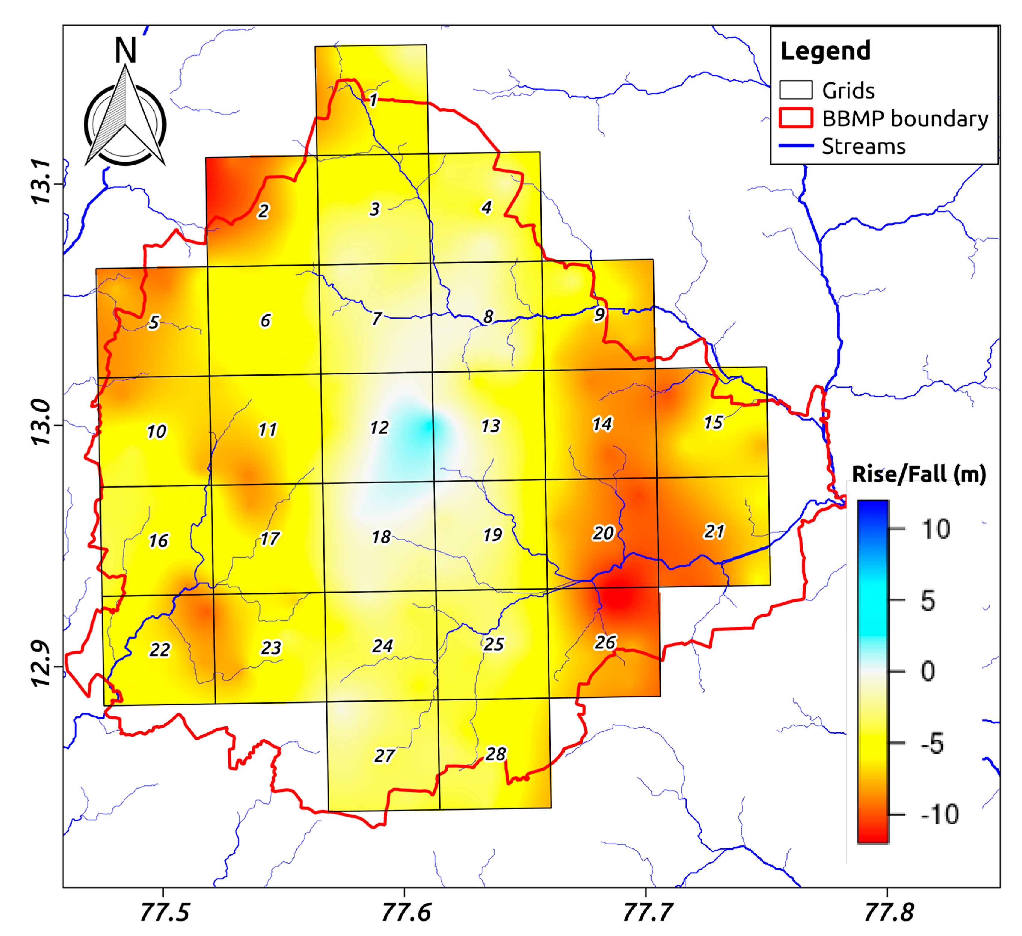
Annual groundwater storage change was computed using the 154 well data and interpolated GWD maps for January 2016 and January 2017 in Equation (5). The change in the groundwater level over this period is shown in Figure 13. Since 2016 was a drought year for Bengaluru city, a significant depletion in the groundwater was observed in entire area except some parts of central Bengaluru (close to grid 12) where a rise of up to 2 m was observed. This area is also highlighted in Mehta et al. [26] who used data from a relatively long-term CGWB monitoring in this area to show the steady rise in GWL over time, and attributed it to the dominance of anthropogenic recharge over pumping. In all other areas, the figure indicates that, due to poor rainfall in 2016, the groundwater level declined by about approximately 12 m in some of the grids, mostly in the outer parts of the city. Estimated mean water storage depleted in the 700 km2 area of the city for 2016 was about 26.9 mm (18.8 million cubic meters) based on the data of 154 wells and 26.2 mm (18.3 million cubic meters) based on the interpolated data. The standard deviation over space was found to be about 18 mm based on the data of 154 wells and 11 mm based on the interpolated data. The lower estimate of standard deviation from kriged data could be due to the presence of nugget in the variogram, which smoothens the data.
3.4. Extreme Rainfall Response
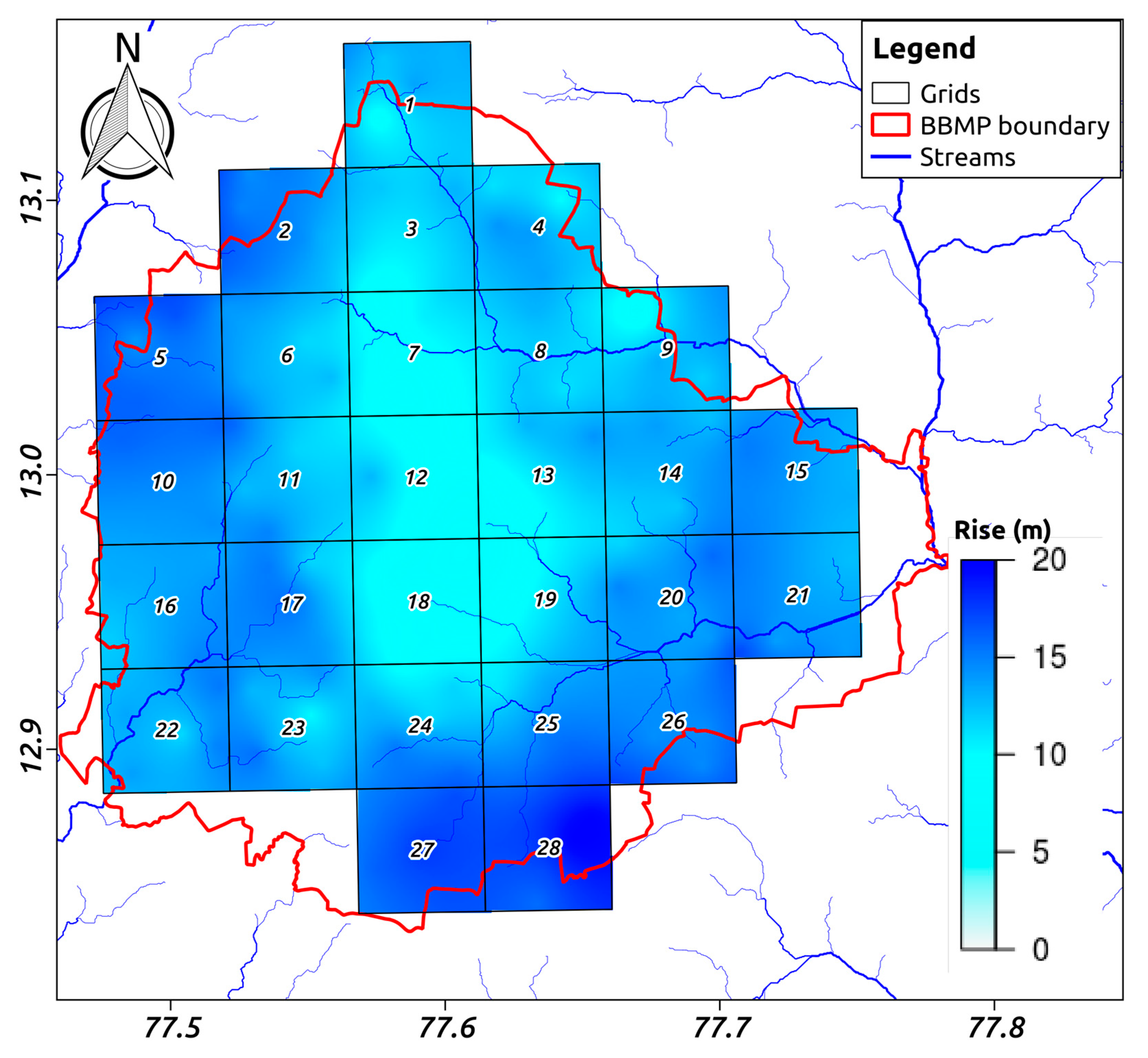
A total of 740.7 mm rainfall was received during August–September, 2017. The recharge from these extreme rainfall events over these two months was estimated using Equation (5). Figure 14 shows the differenced groundwater level map between July 2017 and September 2017. Interestingly, the highest rise is observed in outer grids (Cluster 1) and lowest rise is observed in inner grids (Cluster 3). These outer clusters are in low-lying areas, whereas the central areas are at higher elevation and more densely built-up. A higher fraction of extreme rainfall likely runs off towards the outer areas, where relatively more recharge from the extreme rainfall occurs.
The boxplots (Figure 8) show that GWLs were falling in 2017 through June and July, when monsoon rains were less than normal. Interestingly, the data also show that the extremely high rainfall that immediately followed, during August–September 2017 (see Figure 6), resulted in a quick recharge of groundwater levels in all the stations spread over the city. Average rise in GWL in September 2017 from that of July 2017 was 13.3 m across 154 monitoring wells, while the lowest recorded was 2.6 m (in grid 19) and highest recorded was 24.2 m (in grid 28). The mean rise of 13.3 m due to the rainfall during August–September 2017 had a relatively low standard deviation (over space) of about 4.0 m. During this period, a mean recharge of 66.5 mm for the entire city and a peak recharge of 121 mm (in Grid 28) in some areas were observed. The mean recharge estimate based on the kriged map data also showed nearly the same mean estimate (65.4 mm). However, there was significant difference in the standard deviation over space, 20 mm over 154 wells versus 8.29 mm from interpolated data, owing to the presence of nugget in the data. These two months resulted in a net recharge (increase in net groundwater storage) of about 46.6 million m3 (or 46.6 billion liters) in the 700 km2 of the city.
The recharge generated by these extreme events (rainfall of August–September 2017) is similar to the annual recharge in some agricultural areas in semiarid tropical conditions [15,30]. This suggests that groundwater recharge from extreme rainfall is quite significant in Bengaluru, despite being predominantly built-up. In the literature, significant recharge events from extreme precipitation have been reported [38,39,40] in agricultural regions. In urban areas, however, the conventional narrative is that groundwater recharge is impeded by the dominance of built-up, impervious areas (e.g., [27]). Our observations suggest that, also in urban regions, extreme events can play a major role in groundwater recharge. We hypothesize that these recharge conditions are significantly different from those in agricultural areas, where the recharge is often as a non-point source recharge, i.e., recharge distributed across large areas, such as fields. In urban areas, such non-point source recharge is not feasible due to altered land surfaces in the form of paved surfaces and buildings. However, increased runoff from these altered land use conditions caused localized flooding conditions, during extreme rainfall events. Compounded by the poor storm water drainage conditions in urban cities, the flood waters have higher residence times, which result in recharge through pathways such as construction pits, ponds, storm water drains, and rainwater harvesting structures—the “indirect recharge pathways” that Lerner [4] alludes to as one of the impacts of urbanization. Hence, the recharge would be substantial, and quick, as observed here.
4. Conclusions and Future Improvements
In this paper, we have described the monitoring network and groundwater dynamics across a city, highlighting some of the key findings. First, estimates of groundwater storage changes were made using a simplified, vertical balance. The monitoring will be continued until December 2017. This will provide an opportunity to make groundwater level observations for two monsoon and two non-monsoon seasons during the study period.
One limitation of this study is that only a vertical and simplified estimate of net outflow was made. This net outflow term aggregates both natural and anthropogenic components. To understand the urban groundwater budget more completely, a more elaborate modeling framework would need to include the magnitude of lateral flow and baseflow, for example, as well as the socioeconomic and infrastructural variables that inform the anthropogenic forcings of recharge from leaking pipes and return flows, and draft from pumping. We are working on such a framework, which is briefly described below.
Park and Parker [41] developed a physically based lumped model to simulate groundwater fluctuations in response to precipitation. This model is applicable to estimate groundwater recharge from the observed groundwater level fluctuations as well as groundwater discharge or underflow. One of the limitations of the Park and Parker model is that no external sources or sinks other than uniformly distributed precipitation was considered. Hence, if groundwater pumping exists, then the model needs a suitable adaptation. To use this model for regions with groundwater pumping conditions, Kumar [42] improved the model by taking groundwater pumping into account, which was tested for various conditions by Subash et al. [16]. This improved model (ambhasGW) is available in R (https://cran.rproject.org/package=ambhasGW) for ease of use and to estimate parameters of recharge, discharge, and specific yield from the time series of groundwater level observations. The model provides balance terms of recharge, underflow (or groundwater discharge) and pumping as output. We are currently working on applying this model, and collecting additional socioeconomic and infrastructure data to inform it. To account for the considerable uncertainty in the anthropogenic forcings, we will be applying a formal uncertainty framework, the Generalized Likelihood Uncertainty Framework (GLUE), with the model [43].
More work will be needed to establish the evidence base for these future model outputs. For example, the source of the recharge to groundwater in urban areas could be identified through water chemistry and solute mass balance methods [44,45]
Sustainable groundwater management in Bengaluru must account for substantial spatial socio-hydrological heterogeneity. Continuous monitoring at high spatial density will be needed to inform evidence-based policy. Variables in addition to groundwater levels will need to be monitored for identifying sources and flow paths, and linked to their possible anthropogenic drivers.
Supplementary Materials
The data used in the analysis is available at http://bangalore.urbanmetabolism.asia/geoportal/.
Acknowledgments
Research funding from the Cities Aliance Catalytic Fund is gratefully acknowledged. Funds for open access publishing were provided by the corresponding author’s organizational resources. We also thank Manish Gautam, Deepak Malghan and Krishnachandran Balakrishnan for access to some of the secondary data.
Author Contributions
M. Sekhar and Vishal K. Mehta conceived and designed the experiments; M. Sekhar led the groundwater measurements campaign; M. Sekhar, Sat Kumar Tomer and Vishal K. Mehta analyzed the data and wrote the paper; S. Thiyaku and Sanjeeva Murthy performed the GIS processing and mapping; P. Giriraj and Sanjeeva Murthy measured the groundwater levels; and Vishal K. Mehta was the principal investigator of the research project.
Conflicts of Interest
The authors declare no conflict of interest.
References
- Kumar, M.D.; Shah, T. Groundwater Pollution and Contamination in India: The Emerging Challenge; IWMI-TATA Water Policy Program: Gujarat, India, 2006. [Google Scholar]
- Foster, S.; Hirata, R.; Misra, S.; Garduno, H. Urban groundwater use policy: Balancing the benefits and risks in developing nations. In GW-MATE Strategic Overview Series; World Bank: Washington, DC, USA, 2010; Volume 3. [Google Scholar]
- Eckstein, G.E.; Eckstein, Y. A hydrogeological approach to transboundary ground water resources and international law. Am. Univ. Int. Law Rev. 2003, 19, 201–258. [Google Scholar]
- Lerner, D.N. Identifying and quantifying urban recharge: A review. Hydrogeol. J. 2002, 10, 143–152. [Google Scholar] [CrossRef]
- Onodera, S.I.; Saito, M.; Sawano, M.; Hosono, T.; Taniguchi, M.; Shimada, J.; Umezawa, Y.; Lubis, R.F.; Buapeng, S.; Delinom, R. Effects of intensive urbanization on the intrusion of shallow groundwater into deep groundwater: Examples from Bangkok and Jakarta. Sci. Total Environ. 2008, 404, 401–410. [Google Scholar] [CrossRef] [PubMed]
- Hayashi, T.; Tokunaga, T.; Aichi, M.; Shimada, J.; Taniguchi, M. Effects of human activities and urbanization on groundwater environments: An example from the aquifer system of Tokyo and the surrounding area. Sci. Total Environ. 2009, 407, 3165–3172. [Google Scholar] [CrossRef] [PubMed]
- Gattinoni, P.; Scesi, L. The groundwater rise in the urban area of Milan (Italy) and its interactions with underground structures and infrastructures. Tunn. Undergr. Space Technol. 2017, 62, 103–114. [Google Scholar] [CrossRef]
- Gburek, W.; Folmar, G.; Urban, J. Field data and ground water modeling in a layered fractured aquifer. Groundwater 1999, 37, 175–184. [Google Scholar] [CrossRef]
- Kim, Y.Y.; Lee, K.K.; Sung, I. Urbanization and the groundwater budget, metropolitan Seoul area, Korea. Hydrogeol. J. 2001, 9, 401–412. [Google Scholar] [CrossRef]
- Rao, S.M.; Sekhar, M.; Rao, P.R. Impact of pit-toilet leachate on groundwater chemistry and role of vadose zone in removal of nitrate and E. coli pollutants in Kolar District, Karnataka, India. Environ. Earth Sci. 2013, 68, 927–938. [Google Scholar] [CrossRef]
- Bauer, S.; Bayer-Raich, M.; Holder, T.; Kolesar, C.; Müller, D.; Ptak, T. Quantification of groundwater contamination in an urban area using integral pumping tests. J. Contam. Hydrol. 2004, 75, 183–213. [Google Scholar] [CrossRef] [PubMed]
- Tellam, J.H.; Rivett, M.O.; Israfilov, R.G. Towards management and sustainable development of urban groundwater systems. In Urban Groundwater Management and Sustainability; Springer: Dordrecht, The Netherlands, 2006; pp. 1–9. [Google Scholar]
- Narain, S.; Pandey, P. Excreta Matters: How Urban India Is Soaking up Water, Polluting Rivers and Drowning in Its Own Waste; Centre for Science and Environment: New Delhi, India, 2012. [Google Scholar]
- Planning Commission, Government of India. 12th Five Year Plan (2012–2017); Sage Publications: Thousand Oaks, CA, USA, 2013; Volume I.
- Maréchal, J.C.; Dewandel, B.; Ahmed, S.; Galeazzi, L.; Zaidi, F.K. Combined estimation of specific yield and natural recharge in a semi-arid groundwater basin with irrigated agriculture. J. Hydrol. 2006, 329, 281–293. [Google Scholar] [CrossRef]
- Subash, Y.; Sekhar, M.; Tomer, S.K.; Sharma, A.K. A framework for assessment of climate change impacts on the groundwater system. In Sustainable Water Resources Management; LaMoreaux, J.W., Voss, C.I., Green, N., McCarley, A., Eds.; American Society of Civil Engineers (ASCE): Reston, VA, USA, 2017; Chapter 14. [Google Scholar]
- Drangert, J.O.; Cronin, A. Use and abuse of the urban groundwater resource: Implications for a new management strategy. Hydrogeol. J. 2004, 12, 94–102. [Google Scholar] [CrossRef]
- Öngen, A.; Tinmaz, E. Evaluation of groundwaterover-abstraction by industrial activities in the Trakya region, Turkey. In Urban Groundwater Management and Sustainability; Springer: Dordrecht, The Netherlands, 2006; pp. 117–127. [Google Scholar]
- Wolf, L.; Klinger, J.; Held, I.; Hötzl, H. Integrating groundwater into urban water management. Water Sci. Technol. 2006, 54, 395–403. [Google Scholar] [CrossRef] [PubMed]
- Srinivasan, V.; Gorelick, S.M.; Goulder, L. A hydrologic-economic modeling approach for analysis of urban water supply dynamics in Chennai, India. Water Resour. Res. 2010, 46. [Google Scholar] [CrossRef]
- Sekhar, M.; Shindekar, M.; Tomer, S.K.; Goswami, P. Modeling the vulnerability of an urban groundwater system due to the combined impacts of climate change and management scenarios. Earth Interact. 2013, 17, 1–25. [Google Scholar] [CrossRef]
- Sekhar, M.; Kumar, M.M. Geo-Hydrological Studies Along the Metro Rail Alignment in Bangalore; Technical Report; Department of Civil Engineering, Indian Institute of Science: Bangalore, India, 2009. [Google Scholar]
- Unnikrishnan, H.; Sen, S.; Nagendra, H. Traditional water bodies and urban resilience: A historical perspective from Bengaluru, India. In Water History; Springer: Dordrecht, The Netherlands, 2017; pp. 1–25. [Google Scholar] [CrossRef]
- Mehta, V.; Kemp-Benedict, E.; Goswami, R.; Muddu, S.; Malghan, D. Social ecology of domestic water use in Bangalore. Econ. Political Wkly. 2013, 48. Available online: http://www.epw.in/journal/2013/15/special-articles/social-ecology-domestic-water-use-bangalore.html (accessed on 21 December 2017).
- Farooqi, M. Ground Water Scenario in Major Cities of India; Central Ground Water Board of India: Faridabad, India, 2011.
- Mehta, V.K.; Goswami, R.; Kemp-Benedict, E.; Muddu, S.; Malghan, D. Metabolic urbanism and environmental justice: The water conundrum in Bangalore, India. Environ. Justice 2014, 7, 130–137. [Google Scholar] [CrossRef]
- Hegde, G.V.; Chandra, K.S. Resource availability for water supply to Bangalore city, Karnataka. Curr. Sci. 2012, 102, 1102–1104. [Google Scholar]
- Zimmerman, D.; Pavlik, C.; Ruggles, A.; Armstrong, M.P. An experimental comparison of ordinary and universal kriging and inverse distance weighting. Math. Geol. 1999, 31, 375–390. [Google Scholar] [CrossRef]
- Sun, Y.; Kang, S.; Li, F.; Zhang, L. Comparison of interpolation methods for depth to groundwater and its temporal and spatial variations in the Minqin oasis of northwest China. Environ. Modell. Softw. 2009, 24, 1163–1170. [Google Scholar] [CrossRef]
- Maréchal, J.; Galeazzi, L.; Dewandel, B. Groundwater Balance at the Watershed Scale in a Hard Rock Aquifer Using GIS. In Groundwater Dynamics in Hard Rock Aquifers; Ahmed, S., Jayakumar, R., Salih, A., Eds.; Springer: Dordrecht, The Netherlands, 2008; pp. 134–141. [Google Scholar]
- Balakrishnan, K. Heterogeneity within Indian Cities: Methods for Empirical Analysis. Ph.D. Thesis, University of California, Berkeley, CA, USA, 2016. [Google Scholar]
- Everitt, B.S.; Landau, S.; Leese, M.; Stahl, D. Hierarchical Clustering. In Cluster Analysis, 5th ed.; WILEY: London, UK, 2011; pp. 71–110. [Google Scholar]
- Healy, R.W.; Cook, P.G. Using groundwater levels to estimate recharge. Hydrogeol. J. 2002, 10, 91–109. [Google Scholar] [CrossRef]
- Groundwater Evaluation Committee. Ground Water Resources Estimation Methodology; Ministry of Water Resources, Government of India: New Delhi, India, 1997.
- Ahmed, S.; Jayakumar, R.; Salih, A. Groundwater Dynamics in Hard Rock Aquifers: Sustainable Management and Optimal Monitoring Network Design; Springer Science & Business Media: Dordrecht, The Netherlands, 2008. [Google Scholar]
- Mehta, V.K.; Sekhar, M.; Kemp-Benedict, E.; Sekhar, M.; Mehta, V.K.; Kemp-Benedict, E.; Malghan, D.; Gebbert, S.; Mehta, V.K.; Wang, D.; et al. Groundwater Impacts of water consumption patterns in Bengaluru, India. In Proceedings of the 5th Annual International groundwater Conference, Aurangabad, India, 20 December 2012. [Google Scholar]
- Kumar, D.; Ahmed, S. Seasonal behaviour of spatial variability of groundwater level in a granitic aquifer in monsoon climate. Curr. Sci. 2003, 2, 188–196. [Google Scholar]
- Zhang, J.; Felzer, B.S.; Troy, T.J. Extreme precipitation drives groundwater recharge: The Northern High Plains Aquifer, central United States, 1950–2010. Hydrol. Process. 2016, 30, 2533–2545. [Google Scholar] [CrossRef]
- Taylor, R.G.; Todd, M.C.; Kongola, L.; Maurice, L.; Nahozya, E.; Sanga, H.; MacDonald, A.M. Evidence of the dependence of groundwater resources on extreme rainfall in East Africa. Nat. Clim. Chang. 2013, 3, 374–378. [Google Scholar] [CrossRef] [Green Version]
- Thomas, B.F.; Behrangi, A.; Famiglietti, J.S. Precipitation intensity effects on groundwater recharge in the southwestern United States. Water 2016, 8, 90. [Google Scholar] [CrossRef]
- Park, E.; Parker, J. A simple model for water table fluctuations in response to precipitation. J. Hydrol. 2008, 356, 344–349. [Google Scholar] [CrossRef]
- Kumar, S. Soil Moisture Modelling, Retrieval from Microwave Remote Sensing and Assimilation in a Tropical Watershed. Ph.D. Thesis, Indian Institute of Science, Bangalore, India, 2012. [Google Scholar]
- Beven, K.; Binley, A. The future of distributed models: Model calibration and uncertainty prediction. Hydrol. Process. 1992, 6, 279–298. [Google Scholar] [CrossRef]
- Vázquez-Suñé, E.; Carrera, J.; Tubau, I.; Sánchez-Vila, X.; Soler, A. An approach to identify urban groundwater recharge. Hydrol. Earth Syst. Sci. 2010, 14, 2085–2097. [Google Scholar] [CrossRef] [Green Version]
- Hammami Abidi, J.; Farhat, B.; Ben Mammou, A.; Oueslati, N. Characterization of Recharge Mechanisms and Sources of Groundwater Salinization in Ras Jbel Coastal Aquifer (Northeast Tunisia) Using Hydrogeochemical Tools, Environmental Isotopes, GIS, and Statistics. J. Chem. 2017, 2017, 8610894. [Google Scholar] [CrossRef]
Figure 1.
Spatial distribution (ward-wise) of the population in Bengaluru city. The streams, 5 km × 5 km grid and Telemetric Rainfall Gauge (TRG) of KSNDMC are also shown. Numbers represent the grid-IDs.
Figure 1.
Spatial distribution (ward-wise) of the population in Bengaluru city. The streams, 5 km × 5 km grid and Telemetric Rainfall Gauge (TRG) of KSNDMC are also shown. Numbers represent the grid-IDs.

Figure 2.
Digital Elevation Model (DEM) of Bengaluru city. Numbers represent the grid IDs.

Figure 3.
Percentage of people using groundwater in 2011 (a); and water pipeline network in Bengaluru from 2015 (b).
Figure 3.
Percentage of people using groundwater in 2011 (a); and water pipeline network in Bengaluru from 2015 (b).
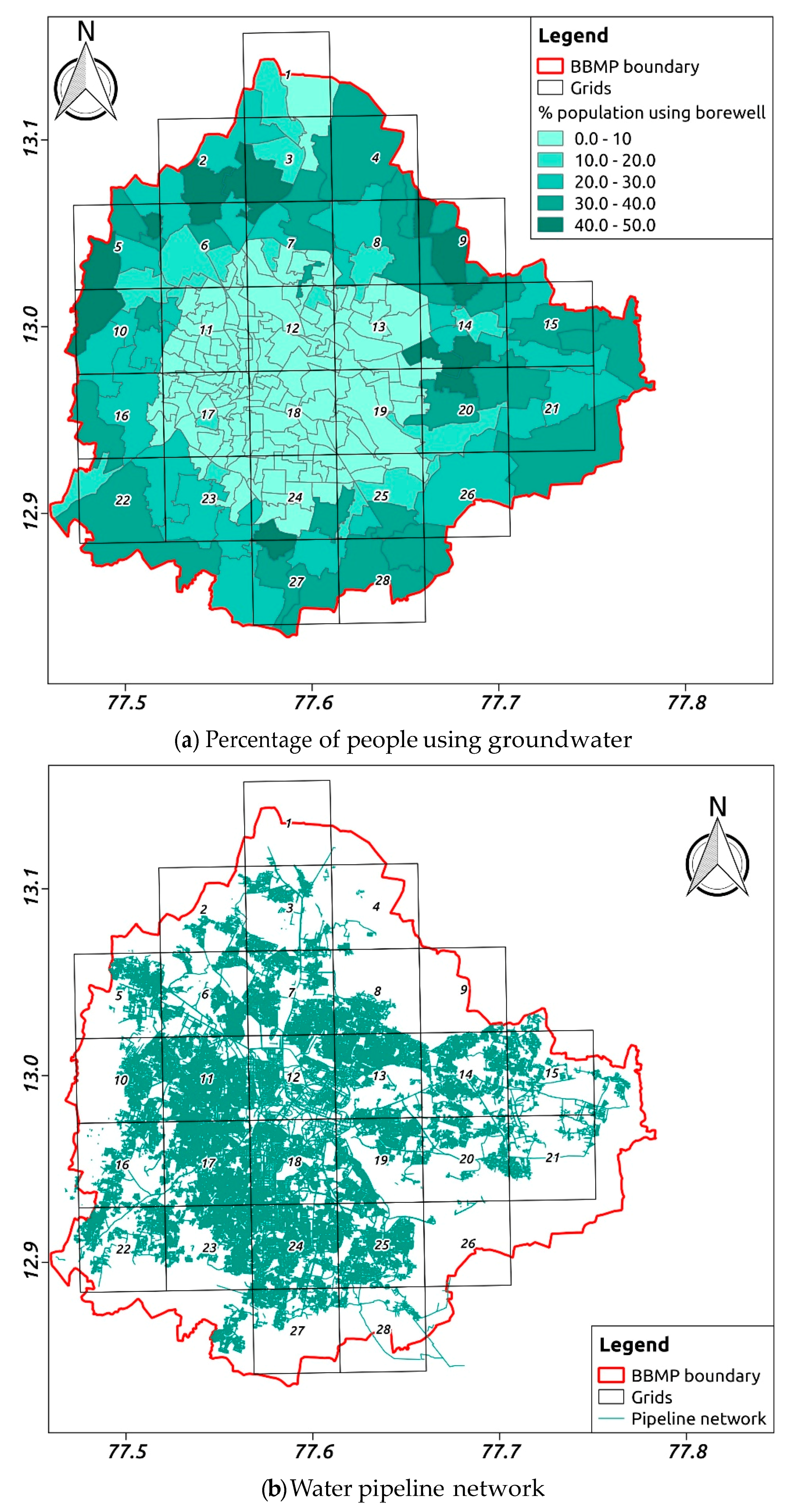
Figure 4.
Spatial distribution of the land cover and monitoring network. Numbers represent the 5 km grid IDs. Landcover data are from 2011 [31].
Figure 4.
Spatial distribution of the land cover and monitoring network. Numbers represent the 5 km grid IDs. Landcover data are from 2011 [31].
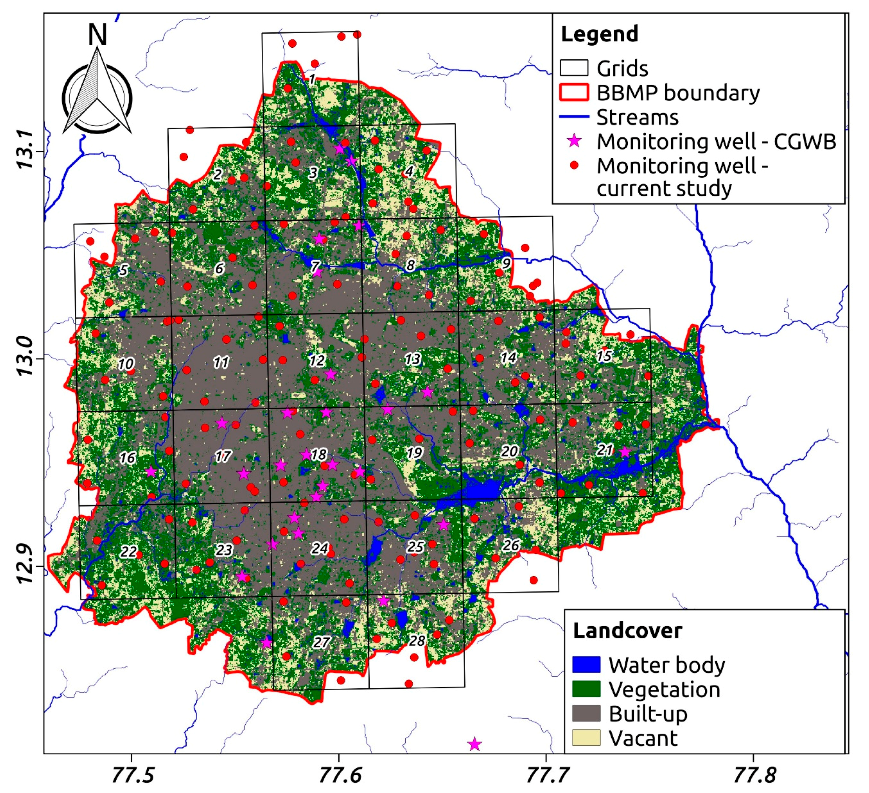
Figure 5.
Annual rainfall in Bengaluru during 1901–2012.
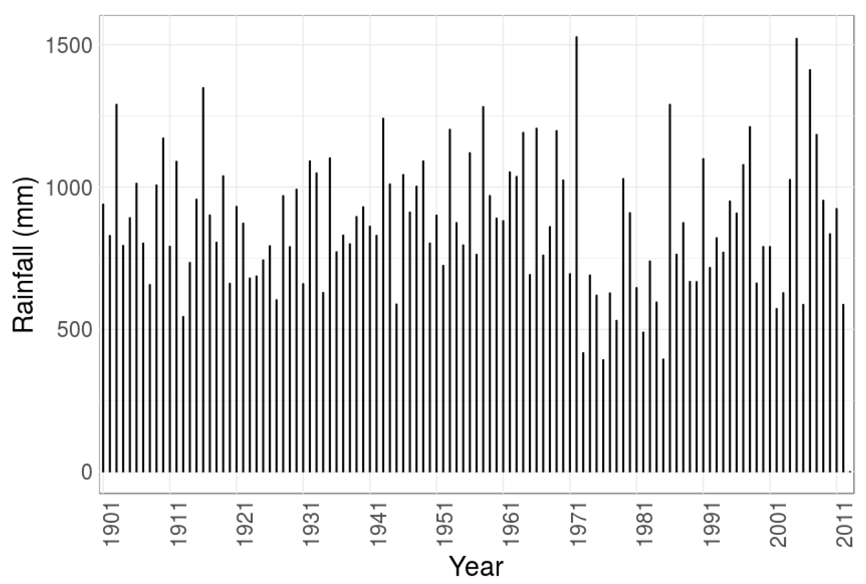
Figure 6.
Monthly rainfall patterns in Bengaluru city during January 2015–October 2017.
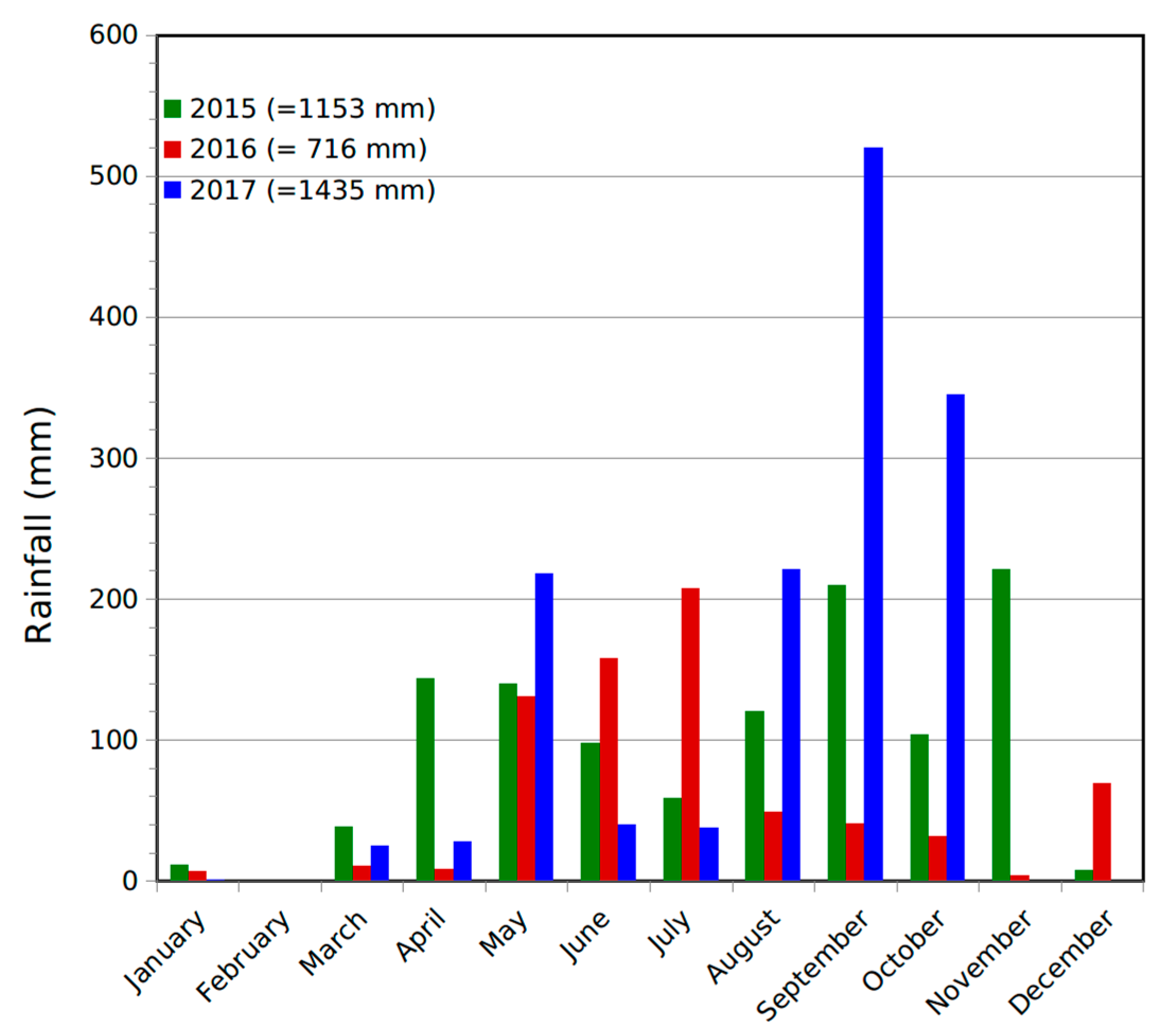
Figure 7.
Dendrogram and spatial distribution of the clusters obtained from Ward’s Linkage algorithm.
Figure 7.
Dendrogram and spatial distribution of the clusters obtained from Ward’s Linkage algorithm.
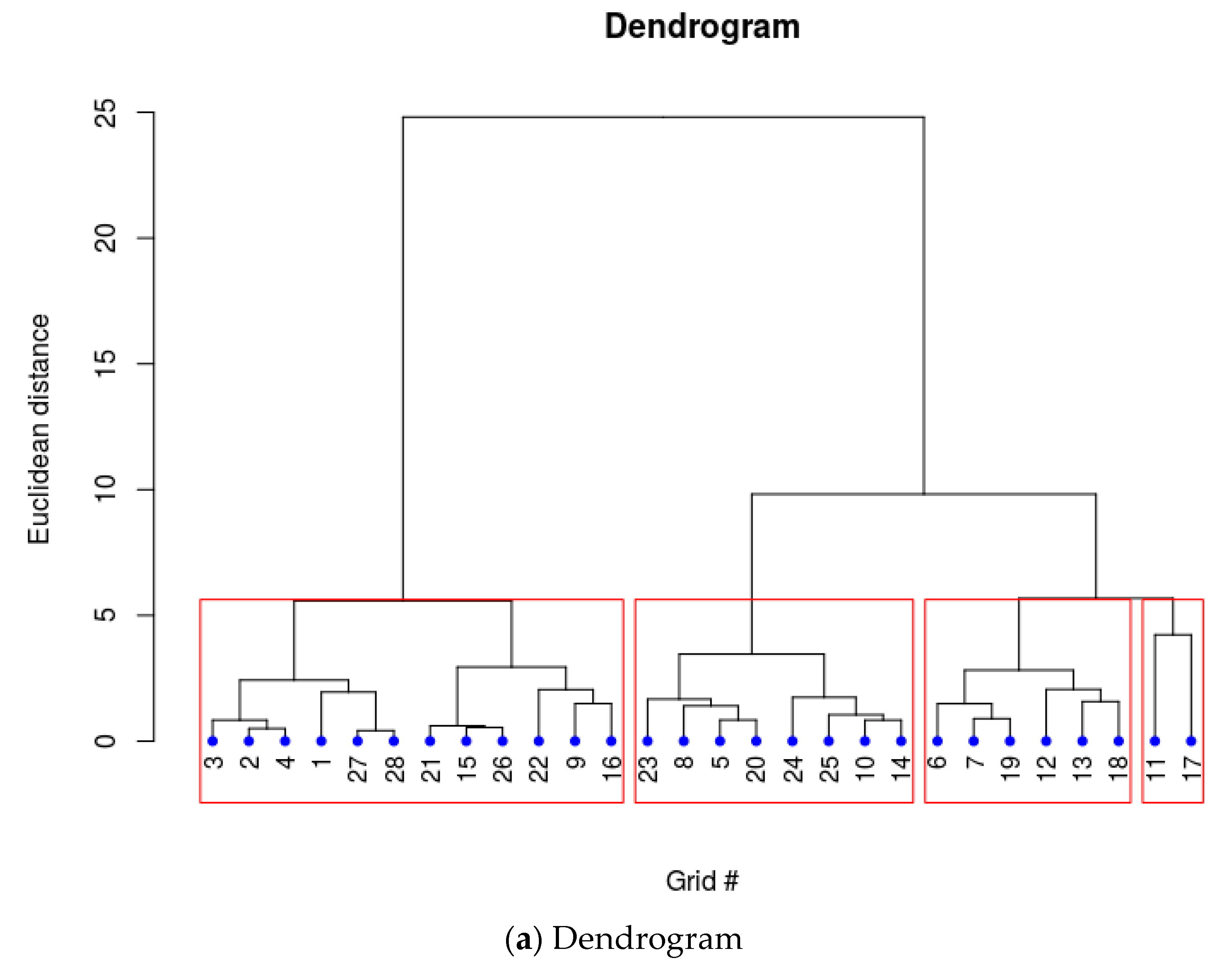

Figure 8.
Box and whisker plot of the DGW of all 154 wells during December 2015–September 2017. The horizontal line within the box indicates the median and boundaries of the box indicate the 25th and 75th percentile. The upper whisker extends from the hinge to the largest value and the lower whisker extends from the hinge to the smallest value.
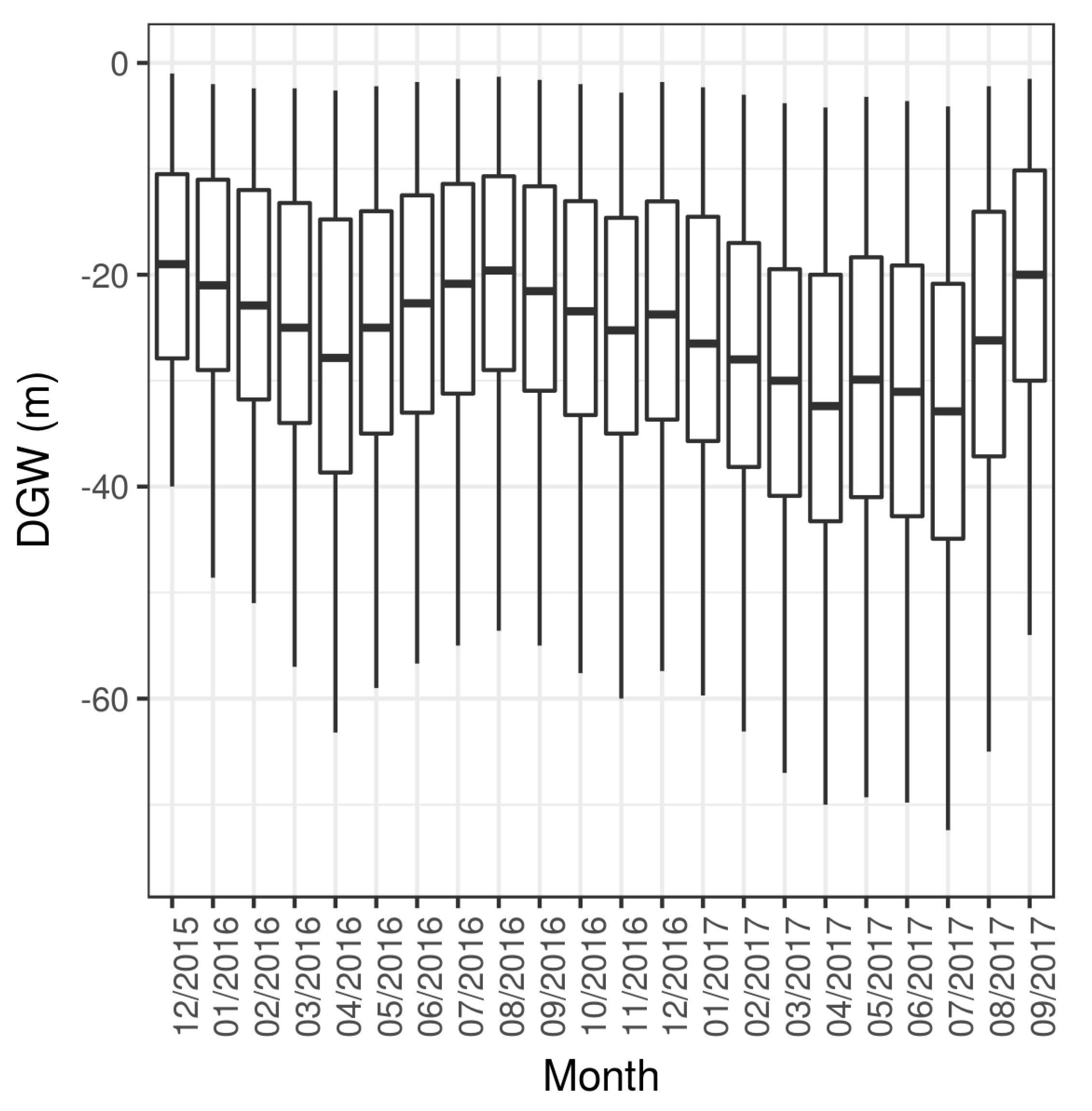
Figure 9.
Box and whisker plots of the depth to groundwater (DGW) of all 154 wells during December 2015–September 2017. The horizontal line within the box indicates the median and boundaries of the box indicate the 25th and 75th percentile. The upper whisker extends from the hinge to the largest value no further than 1.5 × IQR (Inter-Quartile Range) from the hinge. The lower whisker extends from the hinge to the smallest value at most 1.5 × IQR of the hinge. Data beyond the end of the whiskers are called “outlying” points and are plotted individually by filled circle.


Figure 10.
Experimental and fitted exponential variogram for April and August in year 2016.
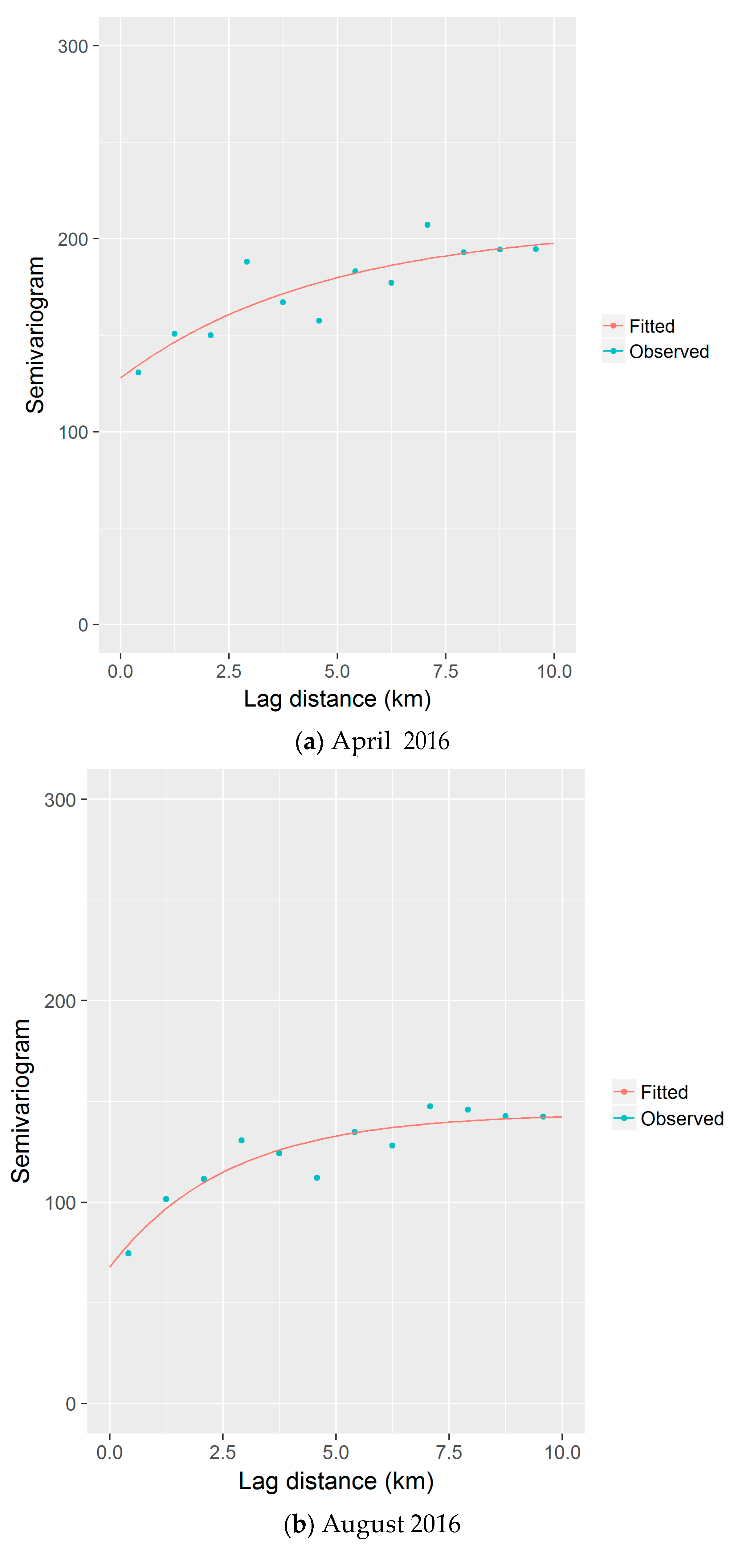
Figure 11.
Interpolated depth to ground water table for selected months during December 2015–September 2017.
Figure 11.
Interpolated depth to ground water table for selected months during December 2015–September 2017.

Figure 12.
Sensitivity analysis of rainfall recharge factor (RF) to specific yield. Shaded region shows the spatial variability over 154 monitoring wells.
Figure 12.
Sensitivity analysis of rainfall recharge factor (RF) to specific yield. Shaded region shows the spatial variability over 154 monitoring wells.

Figure 13.
Difference in the groundwater level between January 2017 and January 2016. Positive numbers indicate rise, and negative numbers indicate fall.
Figure 13.
Difference in the groundwater level between January 2017 and January 2016. Positive numbers indicate rise, and negative numbers indicate fall.

Figure 14.
Rise in the groundwater level from July 2017 to September 2017.


Table 1.
Different variables for each 5 km grid (Relative density of water supply pipeline is computed. using heatmap plugin of QGIS; 1 means highest density and 0 means lowest density).
Table 1.
Different variables for each 5 km grid (Relative density of water supply pipeline is computed. using heatmap plugin of QGIS; 1 means highest density and 0 means lowest density).
| Grid ID | Grid Name | Population | Percentage of Built-Up Area | Elevation (m) | Percentage of People Using Groundwater | Relative Density of Water Supply Pipeline |
|---|---|---|---|---|---|---|
| 1 | Ganganahalli | 76,442 | 15 | 901 | 15 | 0.000 |
| 2 | Vidyaranyapura | 143,937 | 28 | 907 | 28 | 0.063 |
| 3 | Yelahanka New Town | 222,281 | 35 | 905 | 35 | 0.088 |
| 4 | Agrahara | 117,935 | 28 | 919 | 28 | 0.016 |
| 5 | Peenya | 382,500 | 53 | 875 | 53 | 0.130 |
| 6 | Jalahalli | 363,359 | 67 | 914 | 67 | 0.892 |
| 7 | Hebbal | 506,535 | 71 | 892 | 71 | 0.565 |
| 8 | Hennur | 406,705 | 52 | 884 | 52 | 0.323 |
| 9 | Channasandra | 131,351 | 26 | 877 | 26 | 0.015 |
| 10 | Herohalli | 553,028 | 63 | 900 | 63 | 0.065 |
| 11 | Rajajinagar | 984,649 | 94 | 934 | 94 | 1.000 |
| 12 | Bangalore Palace | 525,245 | 89 | 937 | 89 | 0.643 |
| 13 | Cooke Town | 572,268 | 81 | 920 | 81 | 0.318 |
| 14 | Krishnarajapuram | 377,085 | 70 | 902 | 70 | 0.087 |
| 15 | Kodigehalli | 192,238 | 43 | 875 | 43 | 0.043 |
| 16 | Bangalore University | 332,918 | 38 | 851 | 38 | 0.008 |
| 17 | Chamarajpet | 1,048,839 | 92 | 849 | 92 | 0.608 |
| 18 | Shantinagar | 529,064 | 92 | 895 | 92 | 0.675 |
| 19 | Domlur | 395,813 | 69 | 905 | 69 | 0.488 |
| 20 | HAL Airport | 284,738 | 50 | 893 | 50 | 0.178 |
| 21 | Whitefield | 158,578 | 35 | 879 | 35 | 0.075 |
| 22 | Kengeri | 152,050 | 28 | 824 | 28 | 0.033 |
| 23 | Chikkasandra | 514,428 | 66 | 864 | 66 | 0.205 |
| 24 | JP Nagar | 691,729 | 87 | 906 | 87 | 0.146 |
| 25 | HSR Layout | 579,786 | 74 | 887 | 74 | 0.126 |
| 26 | Doddakannelli | 161,190 | 40 | 886 | 40 | 0.002 |
| 27 | Kothnur | 301,144 | 35 | 912 | 35 | 0.047 |
| 28 | Begur | 229,851 | 38 | 911 | 38 | 0.003 |
Table 2.
Details of the clusters formed.
| Cluster ID | Grids | Description |
|---|---|---|
| 1 | 1, 2, 3, 4, 9, 15, 16, 21, 22, 26, 27 and 28 | Outer periphery, lower population density, significant open space, less water supply from BWSSB |
| 2 | 5, 8, 10, 14, 20, 23, 24 and 25 | Inner periphery, moderate population density, moderate open space, moderate water supply from BWSSB |
| 3 | 6, 7, 12, 13, 18 and 19 | Older city core, moderate population density, lower open space, better water supply from BWSSB |
| 4 | 11 and 17 | Highest population density, lower open space, better water supply from BWSSB |
Table 3.
Mean and standard deviation of the R, Qnet and net storage change (R − Qnet) over 154 wells for all the clusters. Numbers in brackets represent the standard deviation.
Table 3.
Mean and standard deviation of the R, Qnet and net storage change (R − Qnet) over 154 wells for all the clusters. Numbers in brackets represent the standard deviation.
| Cluster ID | Qnet (mm) | R (mm) | R − Qnet R (mm) |
|---|---|---|---|
| 1 | 128.89 (84.26) | 100.79 (69.22) | −28.10 |
| 2 | 138.33 (89.12) | 108.79 (73.05) | −29.54 |
| 3 | 86.00 (69.08) | 72.69 (59.89) | −13.31 |
| 4 | 118.85 (46.31) | 84.46 (34.78) | −34.39 |
© 2017 by the authors. Licensee MDPI, Basel, Switzerland. This article is an open access article distributed under the terms and conditions of the Creative Commons Attribution (CC BY) license (http://creativecommons.org/licenses/by/4.0/).
Share and Cite
MDPI and ACS Style
Sekhar, M.; Tomer, S.K.; Thiyaku, S.; Giriraj, P.; Murthy, S.; Mehta, V.K. Groundwater Level Dynamics in Bengaluru City, India. Sustainability 2018, 10, 26. https://doi.org/10.3390/su10010026
AMA Style
Sekhar M, Tomer SK, Thiyaku S, Giriraj P, Murthy S, Mehta VK. Groundwater Level Dynamics in Bengaluru City, India. Sustainability. 2018; 10(1):26. https://doi.org/10.3390/su10010026
Chicago/Turabian StyleSekhar, M., Sat Kumar Tomer, S. Thiyaku, P. Giriraj, Sanjeeva Murthy, and Vishal K. Mehta. 2018. "Groundwater Level Dynamics in Bengaluru City, India" Sustainability 10, no. 1: 26. https://doi.org/10.3390/su10010026
Note that from the first issue of 2016, this journal uses article numbers instead of page numbers. See further details here.