Scale Effects of Water Saving on Irrigation Efficiency: Case Study of a Rice-Based Groundwater Irrigation System on the Sanjiang Plain, Northeast China

Abstract

This research analyzed the scale effect of water saving in Bielahonghe (BLH) Basin, a rice-cultivating district on the Sanjiang Plain, Northeast China. Water budgets with different surface irrigation water supply ratios and water-saving measures were simulated with a semi-distributed water balance model. PF_nws, representing the ratio of rice evapotranspiration to net water supply (the total amount of irrigation and precipitation minus the amount of water reused), was employed to assess the water use efficiency. Seven spatial scales (noted from S1 to S7), ranging from a single field (317.87 ha) to the whole basin (about 100,800 ha) were determined. PF_nws values were quantified across scales and several water-saving measures, including water-saving irrigation regimes, canal lining, and a reduction of the surface water supply ratio (SWSR). The results indicated that PF_nws increased with scale and could be calculated by a fitted power function (PF_nws = 0.736Area^0.033, R² = 0.58). Furthermore, PF_nws increased most prominently when the scale increased from S1 to S2. The water-saving irrigation regime (WSIR) had the most substantial water-saving effect (WSE) at S1. Specifically, PF_nws improved by 21.2% at S1 when high-intensity WSIR was applied. Additionally, the WSE values of S3 and S5 were slightly higher than at other scales when the branch canal water delivery coefficient increased from 0.65 to 0.80 through canal lining. Furthermore, the PF_nws at each scale varied with SWSR. Specifically, PF_nws from S3 to S7 improved as SWSR decreased from 0.4 to 0.3 but remained approximately constant when SWSR decreased from 0.3 to 0.

1. Introduction

As a primary component of water consumption, irrigation is critical to global food production. Growing water scarcity increases the need for water savings, which relies on precise assessments of irrigation efficiency [1,2]. Irrigation efficiency and water savings have become increasingly significant factors in effective agricultural water management [3]. A series of irrigation efficiency indices have been proposed to demonstrate the level of agricultural water management [4,5,6,7,8]. The classic concept of irrigation efficiency (PF_gws) is defined as the ratio of crop evapotranspiration (ET_crop) to the total amount of water inputs (sum of precipitation and irrigation) [9,10]. As it is well known, the applied irrigation (or used irrigation water) ends up as: (1) beneficial evapotranspiration; (2) non-beneficial evapotranspiration; (3) non-recoverable runoff/percolation (e.g., by agriculture, though useful for alternative uses such as the environment); and (4) recoverable runoff/percolation [11]. The first three components constitute the consumed or depleted fraction of irrigation water used, meaning that this water is not available for further use as it is consumed as evapotranspiration, incorporated into a product, or flows to a location where it cannot be readily reused (e.g., heavily saline water). However, the fourth component of the applied irrigation is not consumed and is recoverable for further/later abstractions.

Surface drainage and percolation, which flow from the fields into the drains and groundwater, account for a large proportion of the water inputs [12,13,14]. Water-saving is one of the main objectives to improve irrigation efficiency [15]. Water-saving measures such as drip and sprinkler irrigation, deficit irrigation, and canal lining have been developed and applied in the field to reduce seepage and percolation flows, providing considerable increases in irrigation efficiency [16].

However, irrigation fields are not isolated units but, rather, are part of a whole irrigation system. Water ‘savings’ in one place are likely to reduce return flows to other users (e.g., field) located downstream of the basin [17]. From the perspective of a whole system, a certain amount of so-called lost water (deep percolation, drainage to ditches etc.) may not truly be lost [18]. Outflows at a small scale, such as percolation and drainage, may be reused at a larger scale. ‘Losses’ at the field level can be captured and reused downstream and do not necessarily lead to true water depletion at the irrigation system level. It is necessary to assess whether water ‘saving’ measures are real or only produce local ‘savings’. The irrigation efficiencies in the whole system as well as within river basins are more crucial for agricultural water management [19]. Therefore, water reuse and water-savings quantification at different scales are two important aspects of agricultural water management [20,21,22].

Bos and Wolters [23] found that the high recycling rate of small-scale ‘water loss’ (recoverable runoff/percolation) could improve the water use efficiency of an entire system. It has been argued that irrigation efficiency may increase with increasing spatial scale and may be much higher at the irrigation system level than at the individual field level [24,25]. Because of the different ratios of water reuse, increasing irrigation efficiency through water-saving measures varies at different scales. In addition to the non-linear characteristics of the hydrological processes in the irrigation system, the effects of water savings on irrigation efficiency are scale dependent. Willardson [26] found that the influence of water use efficiency improvements on an individual plot is not significant for watershed-scale efficiency and that water use efficiency improvements at a small scale could lead to either improvements or reductions at a large scale. Molden [27] reported that small-scale and large-scale improvements of water use efficiency are not entirely consistent. Palanisami et al. [28] discovered that improvements in water use efficiency at a point scale do not necessarily indicate improvements in water use efficiency at a large scale. An inaccurate understanding of scale effects can cause confusion when implementing water-saving measures. It is not clear whether the implementation of water-saving irrigation measures at a field scale will produce expected water-saving effects at the basin scale. To select appropriate water-saving irrigation measures and water resource allocation strategies, the scale effects of water use efficiency should be quantitatively studied.

Two main issues must be addressed in such studies. First, conclusions based on the classic index of irrigation efficiency might be incorrect if boundaries at each scale are not correctly understood at the watershed level. Ward and Pulido-Velazquez [29] suggested that the water that is not evaporated and can be recovered should be considered in irrigation efficiency measurements. Keller and Keller [30] noted that effective outflow should be reduced from the water inputs when evaluating irrigation efficiency. However, reusable water is considered, rather than actual water reuse, limiting the quantification of the implementation effect of water-saving technologies. Second, the scale effects of water savings are complicated because the increase in irrigation efficiency should be precisely evaluated after the implementation of water-saving measures.

To evaluate irrigation efficiency and quantify the water savings at different scales, detailed water accounting at corresponding scales should be conducted in advance [31]. The water balance model employs a clear concept and requires few parameters compared with hydrodynamic models such as HYDRUS [32], SWAP [33], and MIKE-SHE [34]; therefore, it is suitable for water budgets with a long time-step in a large region and has been widely used throughout the world [35,36,37,38]. In an irrigation system, the hydrological processes are heavily affected by artificial measures such as crop cultivation, sluice and pump stations, artificial canals and ditches for irrigation and drainage. Due to complicated landscapes with abundant water connections among surface, unsaturated and saturated soil across scales [39], a semi-distributed hydrological model considering the aforementioned physical realities is important to account for the water budget, especially with respect to water reuse. The study area is usually divided into sub-regions to consider spatial variability. A lumped method was employed to create detailed descriptions of water movement in each sub-region which indicated same parameter values were used for specific sub-region. Hydraulic connections among sub-regions were established by identifying water exchanges in groundwater, canals and ditches [40,41]. A semi-distributed physically-based model requires fewer parameters than a distributed model. Hence, it is relatively easy to add physical processes to describe artificial influences on the water cycle, and it is appropriate to analyze the scale effect and water budget in an irrigated area with a semi-distributed model.

In the context of increasing water scarcity, rice has become a main target for water-saving measures considering that 34–43% of the world’s irrigation water is used for rice [42]. Because of the percolation and surface seepage flows from continuously ponded fields into groundwater and drains, seepage and percolation flows account for a large proportion of the water inputs [43,44,45]. The contributions of these flows are particularly high in a rice-based groundwater irrigation system, where a large proportion of groundwater may come from percolation flow. The Bielahonghe (BLH) Basin, located on the Sanjiang Plain, Northeast China, is a rice-based irrigation district that is supplied by groundwater with supplemental irrigation from drainage ditches. In this study, a semi-distributed water balance model was developed and used to account for the components of the water balance. An index of irrigation efficiency considering water reuse was implemented at various scales in the BLH Basin. The scale effects of irrigation efficiency were evaluated, and the contrast with the classic irrigation efficiency index was highlighted. Then, the water budget under different water-saving scenarios (surface irrigation water supply ratios and water-saving measures) was simulated. Water use efficiency and the water reuse fraction at different levels were analyzed, and the scale effects of different water-saving technologies were quantified.

2. Materials and Methods

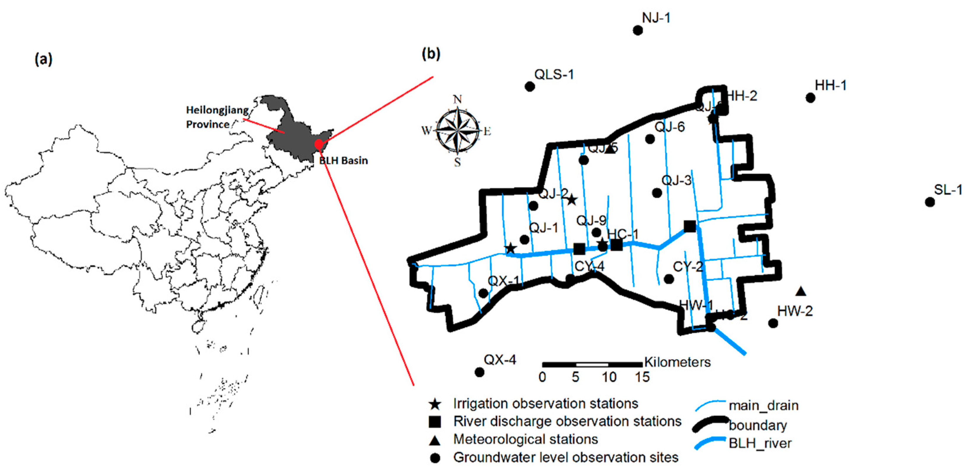
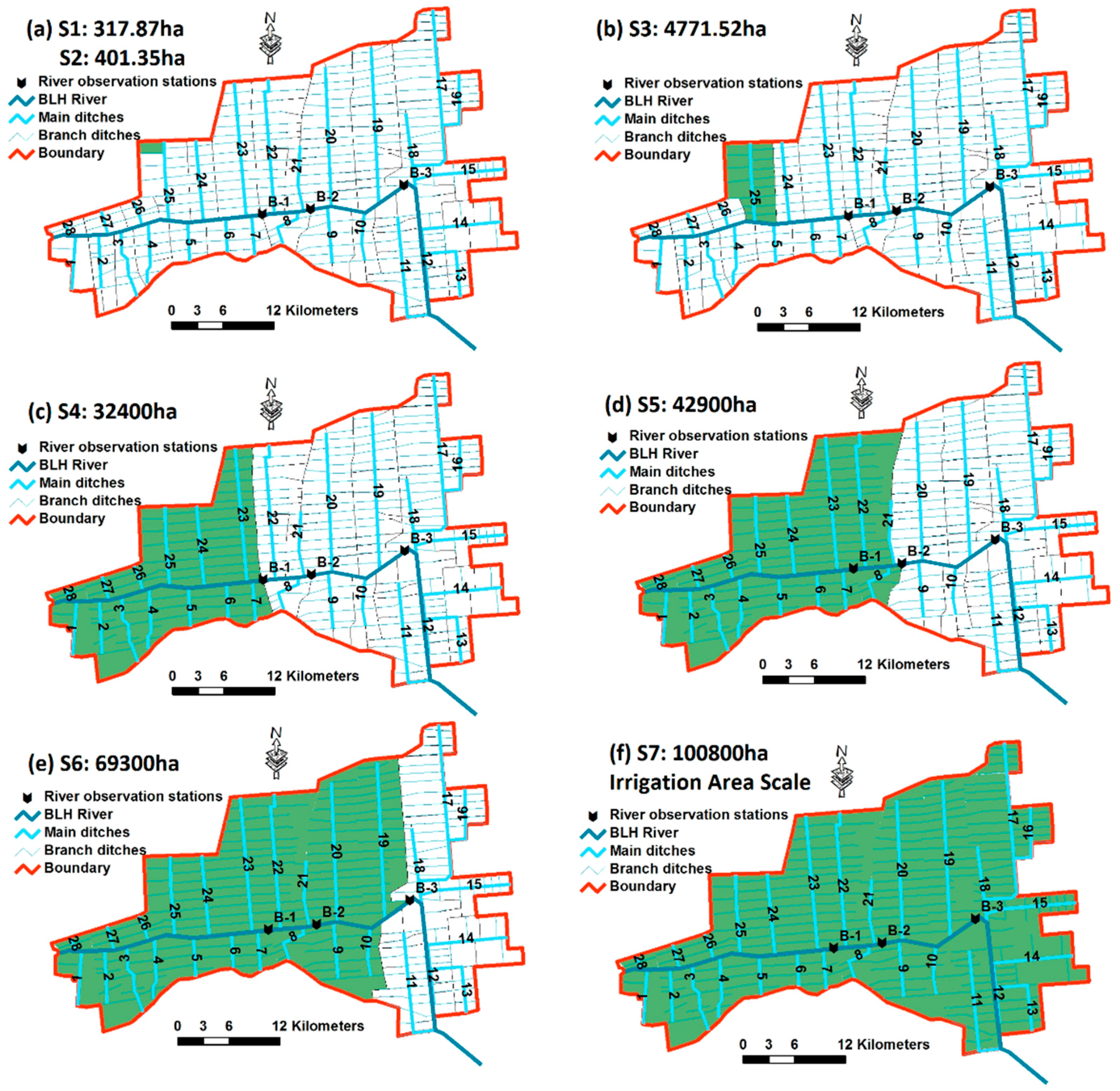
2.1. Study Area and Data

Bielahonghe (BLH) Basin, located on the Sanjiang Plain, Northeast China, is a rice-based irrigation district with an area of 10.08 × 10⁴ ha (Figure 1). The average elevation of this area is 40–50 m, with a slope of 1/5000–1/10,000 and the maximum and minimum elevation are 65 m and 39 m respectively. The study area has a temperate continental monsoon climate with a mean annual temperature of 2.2 °C; the freezing period lasts for up to 120–140 days, and the maximum frozen depth can reach 2.2 m. The average annual precipitation is 545.4 mm, 50–70% of which is concentrated from July to September. Cultivated land covers 69.8% of the study area, and rice is the only crop. Other land use types include forest, grass, bare soils and residential land. Field steeping usually starts in late April; the rice is transplanted in early May and is harvested at the end of September or early October. Groundwater is the dominant source of irrigation water, causing the groundwater table to decline by 37 cm per year. The Quaternary aquifer with a thickness of 180 m is composed of 8–14 m-thick clay loam at the top and sandy loam, sand, and gravel underneath. More exactly, thickness of clay loam of topsoil was higher in west and south when compared with east and north in our study area. Meanwhile, the change of thickness of sand aquifer in the subsoil was opposite. In addition, permeability coefficient changed from 50–60 m/d in west and south to 30–40 m/d in east and north, which was in consistent with the change of elevation. Meanwhile, the horizontal water exchange could be determined based on the monitoring of groundwater in and out of the study region. Drainage system in our study area include three levels of ditches (e.g., lateral ditch, main ditch) and the BLH River. The BLH River collects the drainage from all ditches in the area and flows from west to east to the outlet of the study area. Due to the irrigation channels are being planned, there is no irrigation channel in our study area presently and the main source for irrigation is groundwater. Although farmers might also use private pumps to lift water from the ditches for irrigation, the amount is quite small in our study. Water-saving scenarios have been planned by the authorities [46,47].

The hydrological, meteorological, pumped irrigation and river flow data from 2010 to 2015 were collected from the Authority of the BLH Basin. (i) Daily meteorological data were collected from three meteorological stations (Figure 1). (ii) Groundwater table data were from 20 groundwater table observation wells in the study area (Figure 1). Fourteen (four original sets and ten new sets in August 2014) of these wells were located inside the basin, and six (original ones) were outside the basin. A manual observation method was adopted for the original observation wells with 10-day intervals. An automatic recording method was adopted for new observation wells, and the recording interval was 12 h. (iii) Data on pumped water for irrigation were collected by monitoring typical wells equipped with various motors using a flow-meter to obtain the pumped water quantity. The types and machine power of these typical wells could represent the general conditions for the whole region. Then, we recorded the pumping well distribution map and the horsepower of the equipped motors for the 7400 pumping wells in the study area. The irrigation time in different zones was obtained through the monitoring data from the four wells (Figure 1). Thus, the pumped water amount and irrigation time for all polygonal units (PUs) were determined by accumulating data of wells for specific PU and PU indicated the control area for one ditch (Details about PU were shown in Section 2.2). (iv) For data on river flow, three river flow and level observation stations were established along the BLH River (Figure 1). The water levels in the BLH River were automatically recorded with a water level recorder at 12-h intervals. The river discharge was measured with an LS45-2 current meter to obtain the stage-discharge rating curves. These curves were used to ascertain the river flow changes based on water level records.

The crop coefficients (Kc) were obtained from previous study and root depth of rice was assumed to be 30 cm [48]. The positions of ditches and cross-section parameters were collected from the Qianjin (QJ) Water Administration Bureau. (v) The soil parameters were as follows: soil samples of different depths on 24 selected plots were obtained through drilling, and the soil particle-size distributions were measured. (vi) For hydrogeological parameters, a pumping test was conducted in four plots in October 2014 and March 2015, and the horizontal hydraulic conductivity and specific yields in the aquifer were calculated with test data. (vii) The leaf area index (LAI) at different growth stages were collected from the irrigation experiment station (30 km from the eastern boundary of the study area). In addition, due to the unified management, phenology data (e.g., sowing date, harvest date) and crop cultivar are the same for the study area.

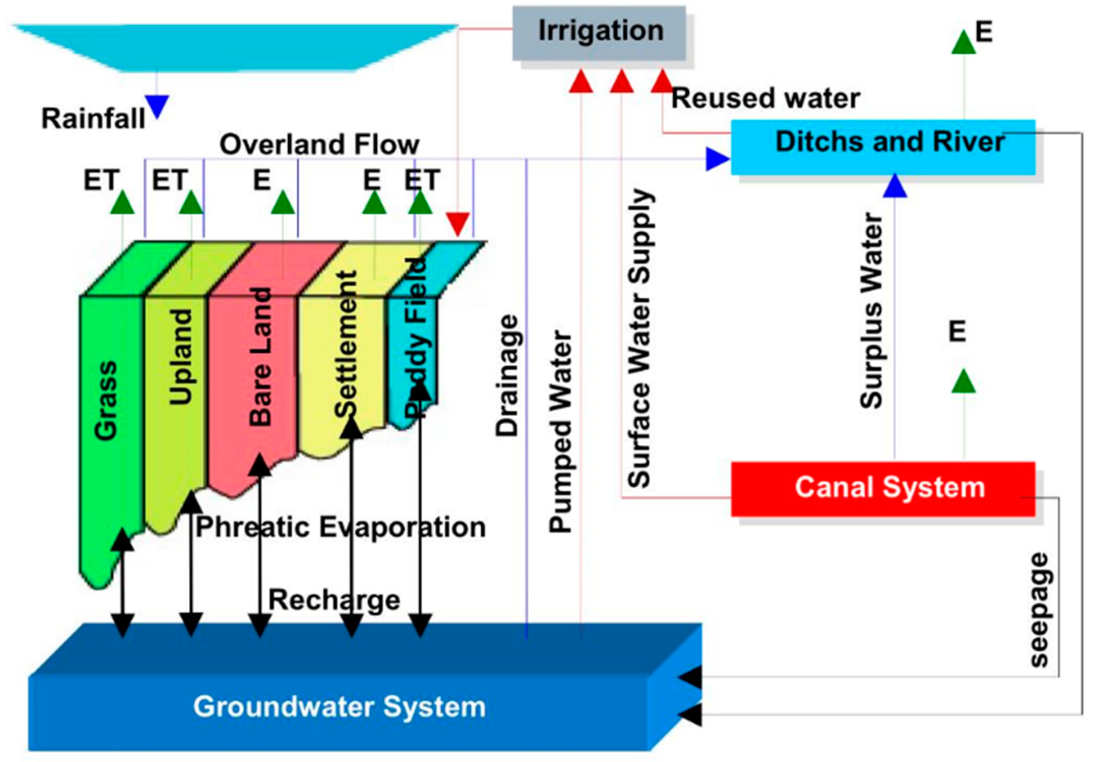
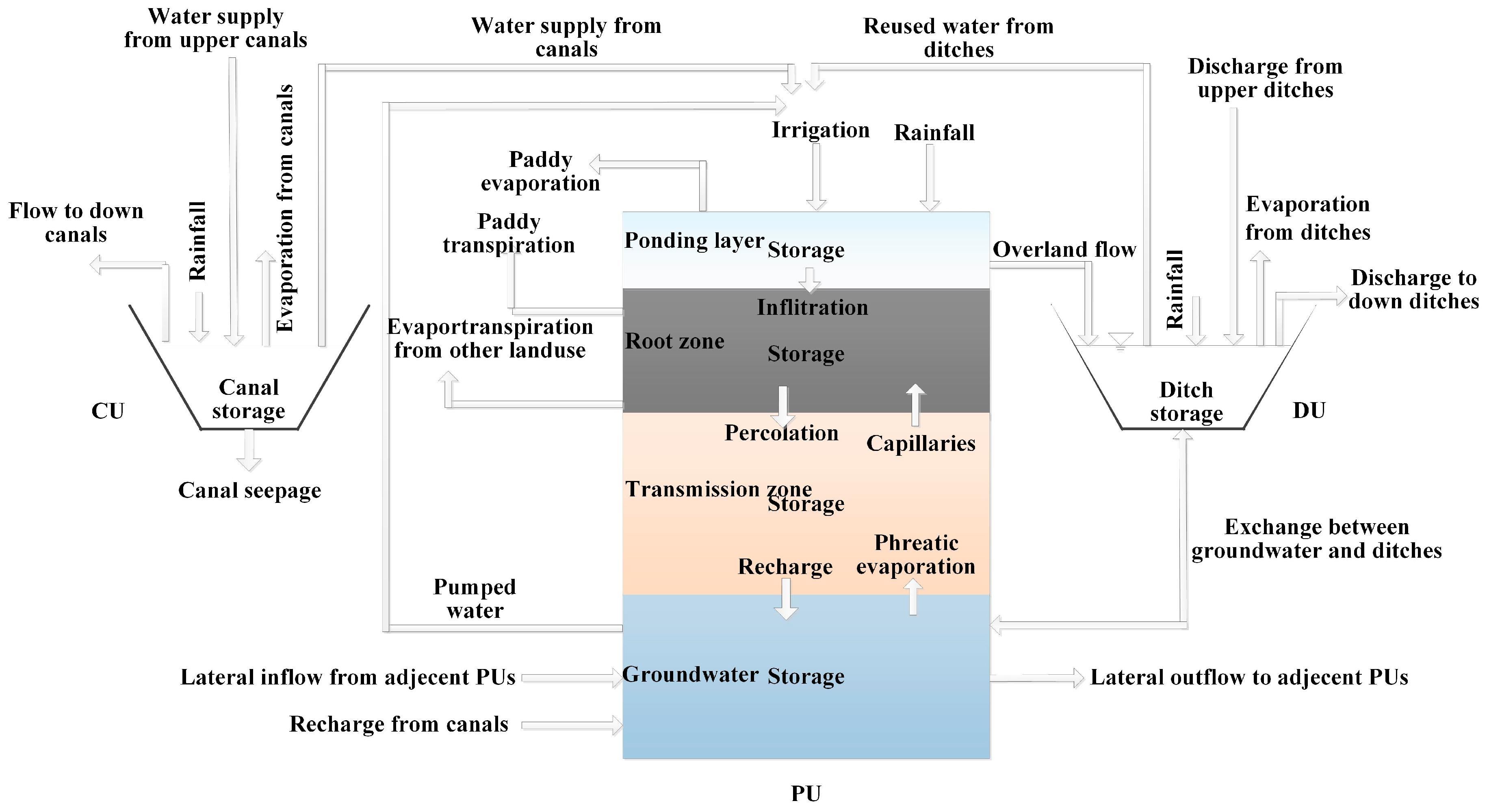
2.2. Distributed Water Balance Model

The distributed water balance model is composed of three types of water balance units: PUs, ditch/river units (DUs), and canal units (CUs). A PU was the total area served by a branch ditch, and five land use types (Figure 2) were considered in a PU. The water budget under various land use types was first simulated; then, the amount of each water balance component in PUs was obtained through accumulation based on the land use area ratio.

Water-transfer relationships among the PUs were established according the distribution of canals and ditches as well as groundwater movement direction (Figure 2 and Figure 3). Canals (CUs) carried out stepwise distribution of water according to the water supply relationship between the upper and lower levels until the PUs were fed through the final-level CUs. After that, a part of PUs’ water flowed into the nearby ditches (DUs) by overland flower, and part of PUs’ water transported downward to the groundwater. Meanwhile, some of groundwater entered into DUs through sub-surface drainage and some exchanged sideways with other PUs’ groundwater by horizontal flow. The overland flow and groundwater drainage from PUs, as well as surplus water from canals, move to branch ditches, then to main ditches, then discharge into the BLH River, eventually flowing out of the study area.

For the water balance in CUs, the amount of rainfall, water diversion from upstream canals, water surface evaporation, water distribution to downstream canals and PUs, and seepage were considered. For the water balance in DUs and the BLH River, the amounts of rainfall, drainage source from up-level ditches and PUs, drainage sinks to down-level ditches, water surface evaporation, reused water, and water interaction with groundwater were involved [49,50].

The soil profile in PUs was divided into a ponding layer, rice root layer, soil water transmission layer, and groundwater layer. The soil water transmission layer was subdivided into a clay layer and sand layer according to the soil texture. After rainfall or irrigation, the water-ponding depth in PUs would increase and water would infiltrate into the rice root layer as the supply for crop evapotranspiration, resulting in changes in soil water content in the rice root layer. When the water content of each unsaturated soil layer exceeded the saturated water content of the corresponding soil layer, the excess water would enter the next layer to recharge the groundwater, causing the groundwater table to increase. Overland flow did not occur until the ponding water depth exceeded the height of the ridge (for non-paddy lands, the ridge height was set to zero). When the ponding water depth in the field (ponding water controlled condition) or the soil water content of the rice root layer (soil water content controlled condition) was below the lower limit of the control, irrigation was performed. The amount of irrigation water was determined by the gap between the upper limit and the lower limit of the ponding water depth (or of the soil water content in the rice root layer) at different growth stages in paddy rice.

The main inputs of the model included the following: meteorological data, water diversion from each canal, irrigation by pumped wells in PUs, crop coefficients at different growth stages and the ratio of crop transpiration and evaporation distribution, control rules for the water layer in different irrigation scenarios, the surface elevation of each PU, the texture distribution and soil properties of the soil profile (saturated water content, field water holding capacity and vertical permeability coefficient), the specific yield and horizontal permeability coefficient of aquifers, the control area and land use ratio of each PU, the geometrical data (length, cross-sectional size) of the ditches and rivers at all levels, the available water utilization coefficient of each canal, the initial groundwater table and the maximum groundwater depth.

The study area was divided into 365 PUs, 365 branch drains and 365 branch canals, 28 main drains and 28 main canals (subdivided into 43 main drain segments and 43 main canal segments), and 1 river (subdivided into 6 river segments). The model was run on a daily scale.

2.3. Water Use Efficiency at Multiple Levels

Recently, the net water supply quantity (irrigation and rainfall minus the amount of reused water) was regarded as the denominator in calculating water use efficiency to reflect the real utilization efficiency of water resources. Therefore, water use efficiency was calculated as follows:

$${\mathrm{PF}}_{\mathrm{nws}}=\frac{{\mathrm{ET}}_{\mathrm{crop}}}{\mathrm{I}+\mathrm{P}-\mathsf{\lambda }}$$

(1)

where λ is the amount of water reuse. In the BLH Basin, irrigation water came partly or wholly from the recycling of surface and subsurface return water (groundwater pumping and drainage reuse for irrigation).

The water reuse fraction (RF) and effective return water fraction (ERFF) were selected to quantify the magnitude of water reuse and outflow outside of the scale boundaries.

$$\mathrm{RF}=\frac{\mathsf{\lambda }}{{\mathrm{Q}}_{\mathrm{CRF}}}$$

(2)

$$\mathrm{ERFF}=\frac{{\mathrm{Q}}_{\mathrm{CRF}}-\mathsf{\lambda }}{{\mathrm{Q}}_{\mathrm{CRF}}}$$

(3)

RF refers to the ratio of water reused to the theoretical return water (Q_CRF), which reflects the extent to which the return water was reused (Equation (2)). If there was no reused water in an irrigation system, the RF was zero. However, if all theoretical return water was reused in a closed irrigation system, the RF was 1. ERFF was defined as the fraction of actual outflow across scale boundaries to the theoretical return water (Equation (3)). A larger ERFF indicated more outflow and little reused water [51,52].

Irrigation and reused water differed in terms of the quantity and connotation at multiple levels (

Table 1. Boundaries and water reuse categories at different scales.

Scale	Horizontal Range	Vertical Range	Items of Water Reuse
S1 (Field Scale)	Rice cultivated area in a PU (canals and ditches excluded)	Root zone	Without reused water
S2	PU (canals and ditches included)	Unsaturated and saturated soil zone	Minimum of pumped water and groundwater recharge in the scale, reused water from ditches in the scale
S3	A main-ditch command area (canals and ditches included)	Unsaturated and saturated soil zone	Minimum of pumped water and groundwater recharge in the scale, reused water from ditches in the scale
S4–S7	Different numbers of main-ditch command areas (canals and ditches included)	Unsaturated and saturated soil zone	Minimum of pumped water and groundwater recharge in the scale, reused water from ditches in the scale

). Therefore, we should define the boundaries of scales and items of irrigation and reused water to determine the water use efficiency at different scales. In this study, seven scales, ranging from a single field to the whole basin were determined, and their horizontal boundaries are shown in Figure 4. Water reuse existed at all scales except S1. In addition, the upward water reuse in S3 and S7 were the smaller value between pump output and groundwater recharge. More exactly, when pump output was larger than groundwater recharge, we could declare that all groundwater recharge was reused. But in the opposite condition, only part of groundwater recharge (pump output) could be reused (Table 1).

2.4. Arrangements of Modeling Scenarios

Parameters including field water capacity, saturated water content, soil water specific yield, and permeability coefficient in our model were firstly calibrated by observed groundwater tables and river discharges from 14 wells and 3 rivers during the growth of paddy rice in 2015. The groundwater tables of 4 wells from 2010 to 2014 were used for model validation. To simulate the effects of water-saving measures on water use efficiency, fifteen scenarios were built by considering three measures: water-saving irrigation regimes, canal lining, and surface water supply ratio (surface water irrigation/total irrigation) reductions. Specifically, two situations were considered as canal water delivery coefficients (real water delivered by canal/water intake in canal head), namely, present and branch canal lining. Three situations of the surface water supply ratio were used: the present condition with a surface water supply ratio of 0, 0.3 and 0.4. The scenario descriptions are presented in

Table 2. Scenario descriptions.

Scenarios	Irrigation Regime	Canal Water Delivery Coefficient	Surface Water Supply Ratio
C1	Present	Presenta	Presentb
C2	Present	Presenta	0.30
C3	Present	Presenta	0.40
C4	Present	Branch canal-0.80, main canal-0.70	0.30
C5	Present	Branch canal-0.80, main canal-0.70	0.40
C6	Low	Presenta	Presentb
C7	Low	Presenta	0.30
C8	Low	Presenta	0.40
C9	Low	Branch canal-0.80, main canal-0.70	0.30
C10	Low	Branch canal-0.80, main canal-0.70	0.40
C11	High	Presenta	Presentb
C12	High	Presenta	0.30
C13	High	Presenta	0.40
C14	High	Branch canal-0.80, main canal-0.70	0.30
C15	High	Branch canal-0.80, main canal-0.70	0.40

Note: Present_a indicates that the water delivery coefficient of branch canals and main canals was 0.65 and 0.70, respectively; Present_b indicates that the surface water supply ratio was 0.

.

The irrigation regimes were classified into the present condition, with low-intensity water saving and high-intensity water saving. The control rules for ponding water depth and soil water content in the root zone under various irrigation regimes are shown in

Table 3. Rules of ponding depth and soil water content for different irrigation regimes (θ_s indicates soil water content at saturation).

Irrigation Regime	Ponding	Green	Early Tillering	Late Tillering	Jointing–Booting	Heading to Flowering	Milk Ripe	Yellow Ripe
Present (mm)	20–55	30–65	30–65	30–65	30–65	30–65	30–65	0–30
Low (mm)	20–50	30–50	30–50	0–50	30–50	10–30	0–30	0–30
High (mm)	20–50	0.9θs–50		0.8θs–θs	0.9θs–30		0.8θs–θs	0.7θs–θs

.

In the scenario simulations, we applied the measured groundwater table, river and ditch water levels on 1 January 2015, and the field capacity as the initial conditions. The daily historical meteorological data from 1956 to 2014 were regarded as the input data driving the model to calculate the water budget and water use efficiency at different scales over 59 years in the study area.

3. Results and Discussion

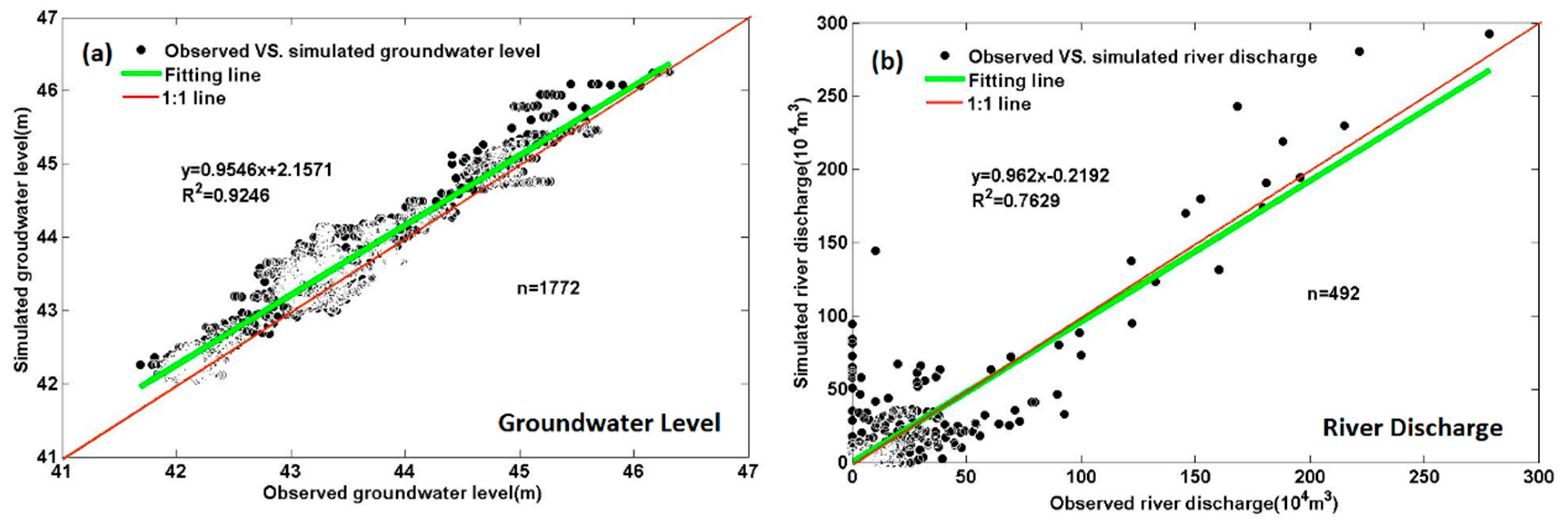
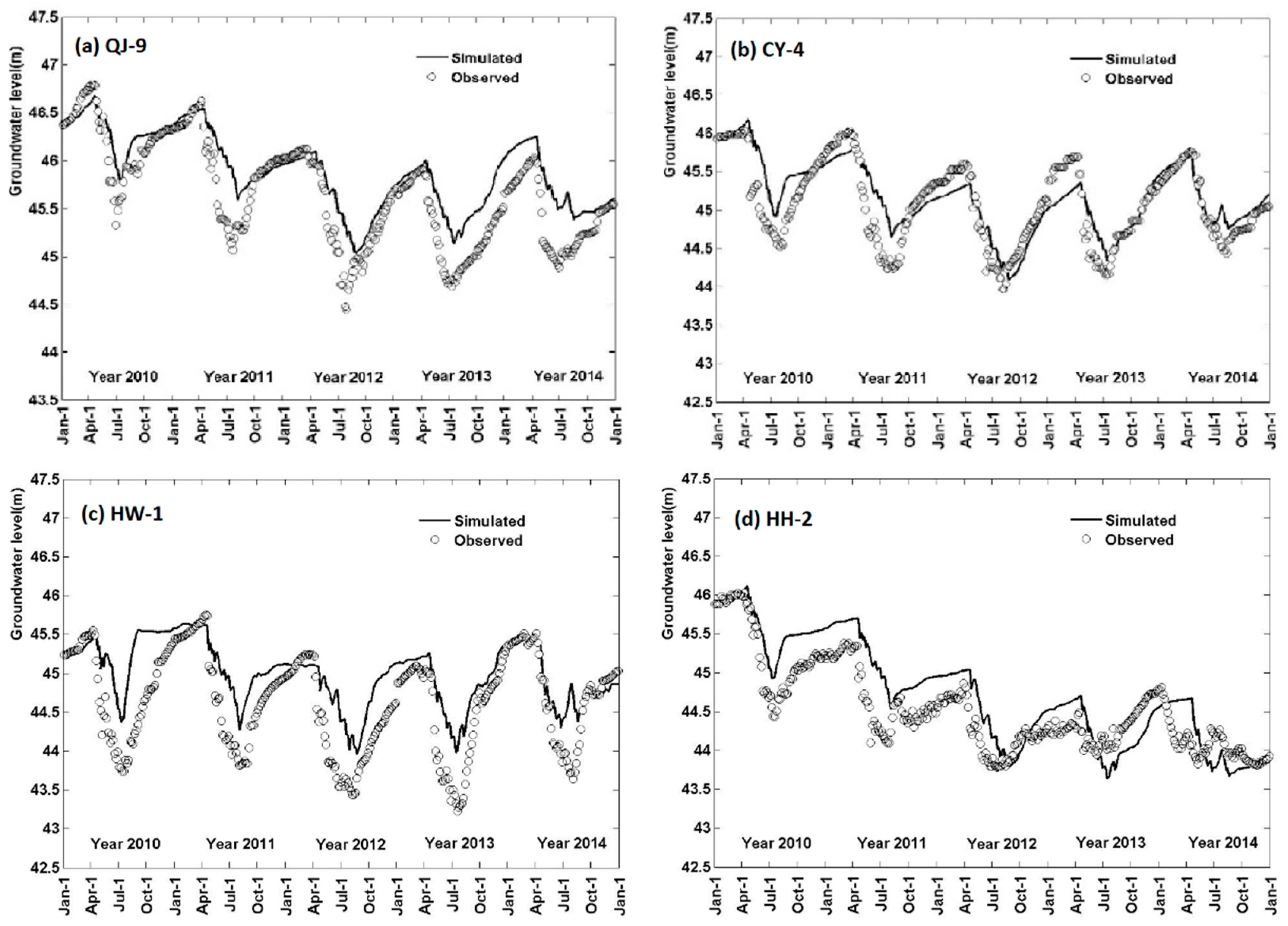
3.1. Water Balance Model Calibration and Validation

A total of 1772 observations of 14 measured groundwater tables and 492 observations of 3 sets of river discharge data during the rice growing period in 2015 were used for model calibration (Figure 5). The R² values of the groundwater table and river discharge between the simulated and observed data were 0.92 (Figure 5a) and 0.76 (Figure 5b), respectively. All pairs of observed and simulated groundwater and river discharge data approximated 1:1 lines (red lines in Figure 5), and the linear-fitting curves (green lines in Figure 5) were also both near 1:1 lines. However, we should point out that the simulation accuracy for river discharge was a little lower than groundwater table (Figure 4). For one thing, there might be some measurement errors for river discharge when the flow velocity is very small. For the other, field drainage after irrigation is one of the main source of river discharge and each study region contains many different fields, there were some bias between the actual irrigation time and the irrigation time inputted in the model, which could also reduce the simulation accuracy for river discharge. In addition, limited weather stations might also reduce the accuracy for our model due to the climatic variability of our experimental area. Therefore, further studies are still needed to improve our model, especially for small velocity conditions.

In the validation process, the time series measurements of 4 groundwater wells from 2010 to 2014 indicated a similar trend between observations and simulations (Figure 6). The R² between the observed and simulated groundwater tables of all 4 groundwater wells (QJ-9, CY-4, HW-1, and HH-2) was 0.8.

Based on the model performance of calibration and validation processes, our established model captured the main characteristics of water balance in our study area. However, we also noted shortcomings in the present study. For example, a slight overestimation of groundwater tables was detected from July to September in QJ-9 and HW-1. This phenomenon might have been caused by two factors. First, the wells for monitoring groundwater tables and pumping for irrigation were usually not located in the same field. Second, due to the huge area of the study site, our model is based on PUs, which is similar with hydrologic response unit (HRU) in SWAT model and the control area is approximately 200 ha; however, the observations for groundwater tables were based on a point scale. Similar issues are found in almost all semi-distributed hydrological models, such as SWAT [53] and SAHYSMOD [54]. However, our model improved the method for identifying HRU (PUs in our study) to bring simulated groundwater tables closer to the observations. Previous hydrological models (e.g., SWAT) usually define HRU based on DEM (Digital Elevation Map) data, while our model focuses on real fields and ditches in an irrigation district. Therefore, PUs in our model were determined based on the minimum control area of each ditch, which made our model more practical and accurate. Besides, water cycle in regional scale is usually very complex and affected by many factors. Lumped model could not consider the spatial variability of these factors while distributed model need too many spatial inputs which are difficult to collect in practice. Our semi-distributed model could balance the advantages and disadvantages between lumped model and distributed model and be more suitable for water cycle simulations in regional scale [55,56,57].

Due to the lack of flow observation points in our validation period (Years: 2010–2014), river discharge data were not available for model validation. Additionally, the dynamics of soil moisture were not measured in our study, although our model could consider this process. However, previous research has indicated that it would be better, but not necessary, to calibrate and validate models for all outputs [58,59]. Therefore, our model is reliable and can be used for further studies on irrigation efficiency under different scenarios at different scales. In the future study, it is necessary to explore the method for obtaining the hydraulic connection among PUs automatically based on the spatial distributions of canal, ditch, field, terrain and so on in the irrigation district. Furthermore, more data about soil, water, and crop in different irrigation district are also needed to evaluate and improve our model.

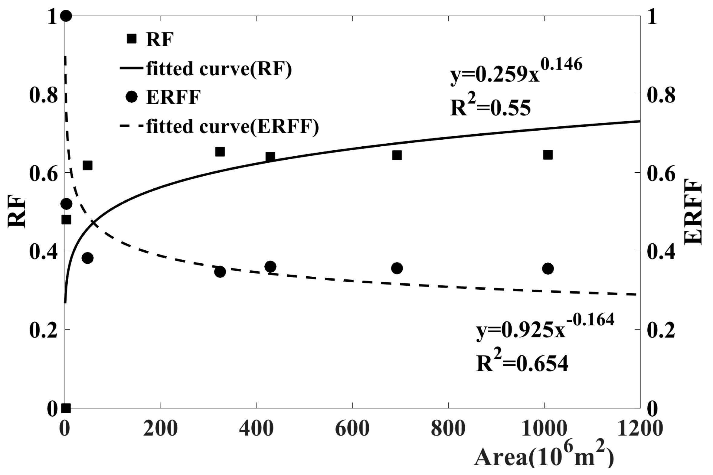
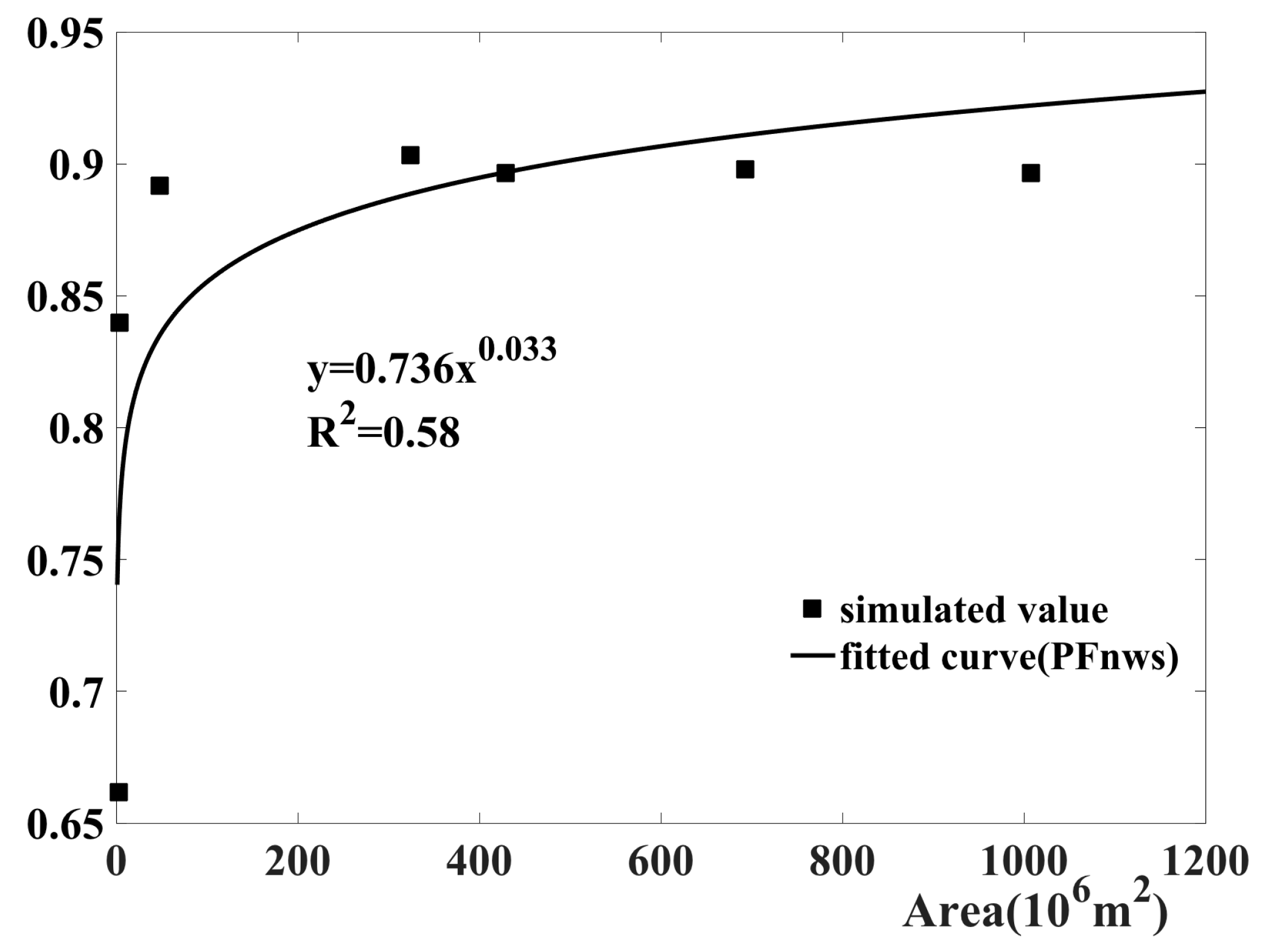
3.2. Current Irrigation Efficiency Across Different Scales

The average water balance components from 2010 to 2015 used to calculate water use efficiency (PF_nws) at different scales are shown in

Table 4. Simulated average water balance components from 2010 to 2015 and water use efficiency across scales.

Scales		S1	S2	S3	S4	S5	S6	S7
Precipitation/mm		522.4	524.5	526.6	528.8	528.7	528.2	528.3
Irrigation/mm	Pumped from groundwater	501.5	397.2	396.1	352.9	338.9	346.4	350.2
	Pumped from ditches	2.1	1.6	2	1.5	1.6	1.7	1.6
	Total irrigation	503.5	398.8	398.1	354.4	340.4	348.1	351.8
ETrice/mm		679	615.8	615.9	581.3	569.3	574.9	578.2
Water reused/mm	From groundwater from Within the scale	0	190	232.1	238.1	232.5	234.4	231.5
	From ditches within the scale	0	0.1	1.9	1.5	1.6	1.7	1.6
	Total water reused	0	190.1	234	239.7	234	236	233.1
Water use efficiency (PFnws)		0.66	0.84	0.89	0.9	0.9	0.9	0.89

Note: All the values in this table are the average of the study area at each scale rather than in the area planted in rice.

. Under the current conditions, groundwater was the dominant irrigation water source, accounting for more than 99% of the total irrigation. Less than 1% of the irrigation water was supplied by drainage water from ditches.

Drainage water and groundwater for irrigation, which were supplied by ditches and saturated aquifers inside the scale boundary, respectively, were considered reused water. Therefore, water from saturated aquifers and ditches located outside the boundary of S1, including irrigation water from groundwater and ditches, was not regarded as reused; therefore, the reused mass was 0. At S2, although 1.622 mm/y irrigation water was derived from drainage, the amount of reused water was only 0.10 mm/y because a large amount of the drainage for irrigation was supplied by ditches outside the S2 boundary. From S4 to S7, all of the drainage water for irrigation was supplied by ditches within the scale boundary; thus, the reused water from ditches was equal to the drainage water for irrigation. From S2 to S7, because groundwater recharge was less than the irrigation pumped from groundwater, the former was considered reused water.

As the scale increased, the RF increased gradually (Figure 7). When the scale moved from S1 to S2, the reuse mass changed from 0 to 190.10 mm/y, which causing the water use efficiency to increase dramatically. As the scale further increased, the amount of reused water gradually increased but at a decelerating growth rate. Meanwhile, the change in ERFF decreased as the scale increased, which was opposite from the change in RF, indicating that the outflow across scales boundaries decreased.

The current PF_nws appeared to exhibit an increasing tendency as the scale increased (Figure 8). The reason was that the outflow regarded as ‘water loss’ in a small scale might be reused at a larger scale, reducing the loss and improving PF_nws as scale increased. Meanwhile, the scale effect of PF_nws could be represented by a power function, which is similar to that reported Xie and Cui [60] but is different from the findings reported by Hafeez et al. [13], who used a linear function to indicate the relationship (Figure 8).

Furthermore, water use efficiency sharply increased (26.9%) when the scale increased from the field scale (S1) to S2 (Figure 8). The reason might be that S1 only contained the surface water layer and the crop root layer, whereas S2 included all of the saturated and unsaturated zones [13].

Furthermore, the dominant reuse of the return water in the study area involved pumped groundwater recharge for irrigation.

The amount of water reuse for calculation of PFnws varied from different scales (Equation (1)). In S1, deep percolation from root zone was regarded as return water and no water reuse in this scale (Table 1). Nevertheless, the return water in S1 can be reused for irrigation in S2 by pumping well. Therefore, water reuse should be considered in S2. Meanwhile, the amount of water reuse from pumping well was very big in S2 (Table 4), which made water use efficiency exhibit the largest increase at this scale. As the scale continued to increase, the water use efficiency did not improve significantly, mainly because the reuse of surface discharge was relatively low in the study area.

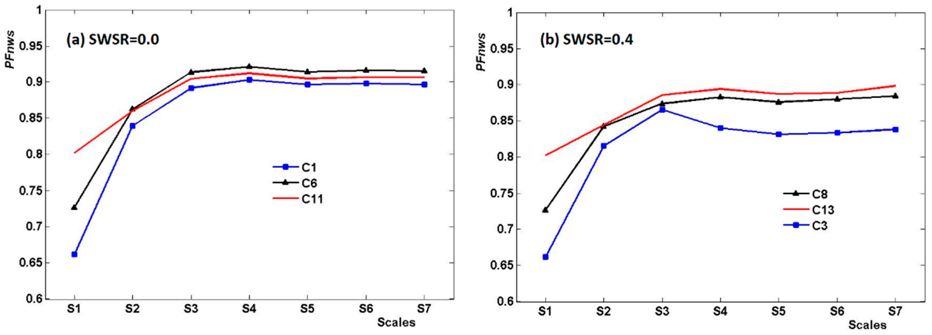
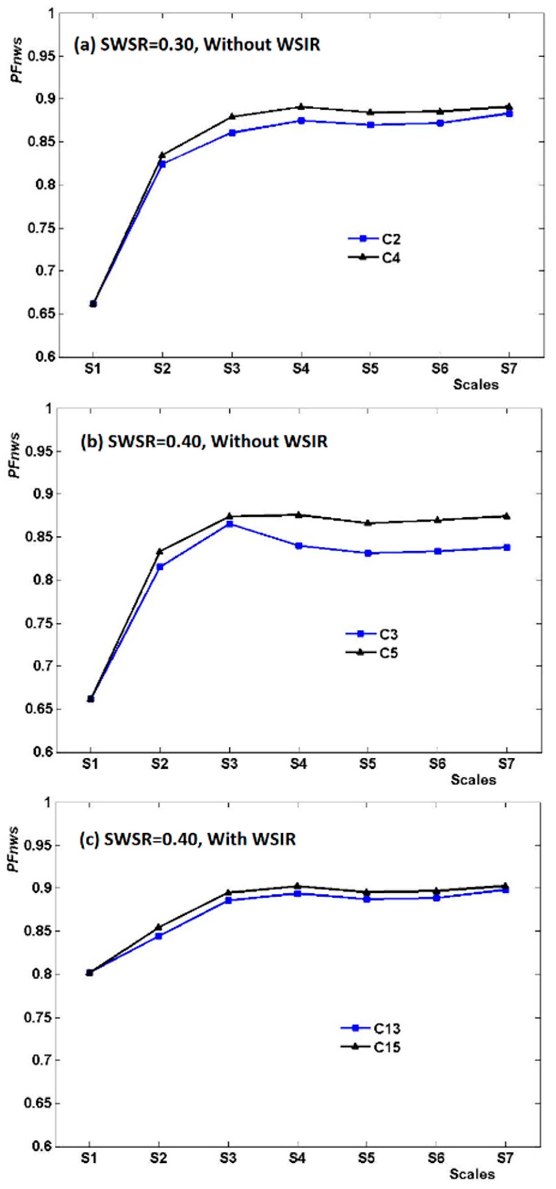
3.3. Scale Effects of Simulated Water-Saving Measures on Irrigation Efficiency

Based on our simulations of different scenarios (Table 2), the influence of different irrigation regimes on water use efficiency (PF_nws) at different scales was as indicated in Figure 9. Water saving irrigation regimes (WSIRs) had the most significant positive effect (an increase by 21.2%) on S1 (field scale) among scales in this study. The water-saving effect (WSE) of WSIR on other scales was influenced by the surface water supply ratio (SWSR). First, without surface water supply (Figure 9a), WSIR provided almost no WSE at scales other than S1. For example, the WSE at S7 (irrigation area scale) was only 1.13% even if high-intensity WSIR was adopted. Second, the WSE at scales from S2 to S7 began to increase with increasing SWSR. When the SWSR reached 0.4 (Figure 9b), the WSE at S7 with the application of a high-intensity WSIR was 7.17%. Third, the difference in WSE at all scales of the low-intensity and high-intensity WSIR was not significant when SWSR was less than 0.4.

WSIR exhibited a relatively substantial WSE at the field scale (S1). The primary reason might be that the amount of reused water was not considered at this scale; thus, water use efficiency (PF_nws) was influenced by the gross water supply (reused water was not considered) [61]. When WSIR was adopted, the gross water supply was reduced, causing an improvement in water use efficiency. Furthermore, at scales other than S1, the reused water was considered. If we ignore the change in ET after applying WSIR at scales from S2 to S7, the water use efficiency was only influenced by the net water supply, which was the gross water supply minus the reused water amount. After WSIR was implemented, decreases in gross water supply and reused water had a positive and negative effect on the improvement of water use efficiency, respectively, and WSE obviously decreased when the effects of the two factors were combined.

When the branch canal water delivery coefficient increased from 0.65 to 0.80 through canal lining, the WSE at scales from S3 (4771.52 ha) to S5 (4.29 × 10⁴ ha) were more obvious than those at other scales (Figure 10a). However, the WSE was less than 2% because of the relatively low SWSR. When the SWSR was 0.4 (Figure 10b), the WSE at scales from S4 (3.24 × 10⁴ ha) to S7 (10.08 × 10⁴ ha) increased slightly, reaching approximately 4.3%. However, the WSE of the canal lining decreased if WSIR was applied (Figure 10c). In this study, when the SWSR was less than 0.4, the WSE of the canal lining at all scales was almost negligible when high-intensity WSIR was adopted.

Based on the above analysis, our simulation results for different scenarios indicated that the influence of water savings and water resources regulation measures on reused water across scales exhibited nonlinear characteristics. Thus, WSE presented complex responses, which were influenced both by recycling of the return flow as well as the responses of water balance components at different scales to water-saving measures [62,63].

4. Conclusions

Our study evaluated the scale effect of water saving in the BLH Basin, a rice cultivation area located on the Sanjiang Plain, Northeast China. Under the current situation, percolation and drainage were regarded as ‘water losses’ at a small scale but were reused by pumping for irrigation. When the scale increased, the RF increased and the ERFF decreased, and water use efficiency exhibited an increased tendency with increased scale, which could be expressed by a power function by the scale area. Furthermore, due to the theoretical return water being reused through pumped groundwater, the water use efficiency improved dramatically when the scale boundary expanded from a crop root layer to the whole unsaturated-saturated soil zone.

The WSE of different water-saving and water resource regulation measures proved to be scale dependent. When the SWSR was zero, the application of WSIR achieved the greatest WSE (21.2%) at S1 of all 7 scales, whereas it resulted in almost no WSE at other scales except S1. However, the WSE of WSIR at other scales, except S1, gradually increased when the SWSR increased. When the branch canal water delivery coefficient increased from 0.65 to 0.80 with canal lining and the SWSR was 0.3, without WSIR, the WSE at scales from S3 to S5 correspondingly improved (<2%). Moreover, the increase in SWSR was enhanced, whereas the WSIR implementation might reduce the WSE of branch canal lining at each scale. Furthermore, the PF_nws at scales larger than S3 began to ascend when the SWSR decreased from 0.4 to 0.3 without WSIR. However, a further reduction in SWSR from 0.3 to 0.1 caused no changes in PF_nws at S1 and S7.

Overall, our study established a semi-distributed water-balance model to consider the effects of crop and human activities on hydrological dynamics at different scales in an irrigation district. Our model was scientifically evaluated for both river discharge (R² > 0.75) and groundwater tables (R² > 0.8). And can be used for evaluating water cycles and water use efficiency at rice cultivation sites. However, due to the complicated mechanisms of water cycle dynamics and the huge spatial data requirements for a real irrigation district, the present model should be improved in certain respects, such as refining the simulation unit, identifying flow directions among units, and representing surface water dynamics processes.

References

1. Seekell, D.; Carr, J.; Dell’Angelo, J.; D’Odorico, P.; Fader, M.; Gephart, J.; Kummu, M.; Magliocca, N.; Porkka, M.; Puma, M.; et al. Resilience in the global food system. Environ. Res. Lett. 2017. [Google Scholar] [CrossRef]
2. Jägermeyr, J.; Gerten, D.; Schaphoff, S.; Heinke, J.; Lucht, W.; Rockström, J. Integrated crop water management might sustainably halve the global food gap. Environ. Res. Lett. 2016, 11, 025002. [Google Scholar] [CrossRef]
3. Ashofteh, P.-S.; Bozorg-Haddad, O.; Loáiciga, H.A. Development of adaptive strategies for irrigation water demand management under climate change. J. Irrig. Drain. Eng. 2017, 143, 04016077. [Google Scholar] [CrossRef]
4. Sun, H.; Wang, S.; Hao, X. An improved analytic hierarchy process method for the evaluation of agricultural water management in irrigation districts of north china. Agric. Water Manag. 2017, 179, 324–337. [Google Scholar] [CrossRef]
5. Pereira, H.; Marques, R.C. An analytical review of irrigation efficiency measured using deterministic and stochastic models. Agric. Water Manag. 2017, 184, 28–35. [Google Scholar] [CrossRef]
6. Yan, Z.; Gao, C.; Ren, Y.; Zong, R.; Ma, Y.; Li, Q. Effects of pre-sowing irrigation and straw mulching on the grain yield and water use efficiency of summer maize in the north china plain. Agric. Water Manag. 2017, 186, 21–28. [Google Scholar] [CrossRef]
7. Wang, Y.B.; Liu, D.; Cao, X.C.; Yang, Z.Y.; Song, J.F.; Chen, D.Y.; Sun, S.K. Agricultural water rights trading and virtual water export compensation coupling model: A case study of an irrigation district in china. Agric. Water Manag. 2017, 180, 99–106. [Google Scholar] [CrossRef]
8. Zhang, H.; Xiong, Y.; Huang, G.; Xu, X.; Huang, Q. Effects of water stress on processing tomatoes yield, quality and water use efficiency with plastic mulched drip irrigation in sandy soil of the hetao irrigation district. Agric. Water Manag. 2017, 179, 205–214. [Google Scholar] [CrossRef]
9. Howell, T.A. Irrigation efficiency. In Encyclopedia of Water Science; Marcel Dekker: New York, NY, USA, 2003; pp. 467–472. [Google Scholar]
10. Giuliani, M.M.; Gatta, G.; Nardella, E.; Tarantino, E. Water saving strategies assessment on processing tomato cultivated in mediterranean region. Ital. J. Agron. 2016, 11, 69–76. [Google Scholar] [CrossRef]
11. Burt, C.M.; Clemmens, A.J.; Strelkoff, T.S.; Solomon, K.H.; Bliesner, R.D.; Hardy, L.A.; Howell, T.A.; Eisenhauer, D.E. Irrigation performance measures: Efficiency and uniformity. J. Irrig. Drain. Eng. 1997, 123, 423–442. [Google Scholar] [CrossRef]
12. Bouman, B.A.M. A conceptual framework for the improvement of crop water productivity at different spatial scales. Agric. Syst. 2007, 93, 43–60. [Google Scholar] [CrossRef]
13. Hafeez, M.M.; Bouman, B.A.M.; Van de Giesen, N.; Vlek, P. Scale effects on water use and water productivity in a rice-based irrigation system (upriis) in the Philippines. Agric. Water Manag. 2007, 92, 81–89. [Google Scholar] [CrossRef]
14. Bouman, B. Water Management in Irrigated Rice: Coping with Water Scarcity; International Rice Research Institute: Los Baños, Philippines, 2007. [Google Scholar]
15. Expósito, A.; Berbel, J. Agricultural irrigation water use in a closed basin and the impacts on water productivity: The case of the guadalquivir river basin (southern Spain). Water 2017, 9, 136. [Google Scholar] [CrossRef]
16. Bouman, B.A.M.; Tuong, T.P. Field water management to save water and increase its productivity in irrigated lowland rice. Agric. Water Manag. 2001, 49, 11–30. [Google Scholar] [CrossRef]
17. Droogers, P.; Kite, G. Water productivity from integrated basin modeling. Irrig. Drain. Syst. 1999, 13, 275–290. [Google Scholar] [CrossRef]
18. Molle, F.; Venot, J.-P.; Lannerstad, M.; Hoogesteger, J. Villains or heroes? Farmers’ adjustments to water scarcity. Irrig. Drain. 2010, 59, 419–431. [Google Scholar] [CrossRef]
19. Expósito, A.; Berbel, J. Sustainability implications of deficit irrigation in a mature water economy: A case study in southern Spain. Sustainability 2017, 9, 1144. [Google Scholar] [CrossRef]
20. Playán, E.; Mateos, L. Modernization and optimization of irrigation systems to increase water productivity. Agric. Water Manag. 2006, 80, 100–116. [Google Scholar] [CrossRef] [Green Version]
21. Bahri, A. Agricultural reuse of wastewater and global water management. Water Sci. Technol. 1999, 40, 339–346. [Google Scholar]
22. Simons, G.W.H.; Bastiaanssen, W.G.M.; Immerzeel, W.W. Water reuse in river basins with multiple users: A literature review. J. Hydrol. 2015, 522, 558–571. [Google Scholar] [CrossRef]
23. Bos, M.; Wolters, W. Project or overall irrigation efficiency. In Proceedings of the International Conference in Irrigation Theory and Practice, Southampton, UK, 12–15 September 1989; Rydzewski, J.R., Ward, C.F., Eds.; Pentech Press: London, UK, 1989; pp. 499–506. [Google Scholar]
24. Tuong, T.P.; Bouman, B.A.M.; Mortimer, M. More rice, less water—Integrated approaches for increasing water productivity in irrigated rice-based systems in Asia. Plant Prod. Sci. 2005, 8, 231–241. [Google Scholar] [CrossRef]
25. Bouman, B.A.M.; Humphreys, E.; Tuong, T.P.; Barker, R. Rice and water. In Advances in Agronomy; Sparks, D.L., Ed.; Academic Press: Cambridge, MA, USA, 2007; Volume 92, pp. 187–237. [Google Scholar]
26. Willardson, L.S. Basin-wide impacts of irrigation efficiency. J. Irrig. Drain. Eng. 1985, 111, 241–246. [Google Scholar] [CrossRef]
27. Molden, D. Accounting for Water Use and Productivity; International Water Management Institute: Colombo, Sri Lanka, 1997. [Google Scholar]
28. Palanisami, K.; Senthilvel, S.; Ramesh, T. Water Productivity at Different Scales under Canal, Tank and Well Irrigation Systems; International Water Management Institute: Colombo, Sri Lanka, 2009. [Google Scholar]
29. Ward, F.A.; Pulido-Velazquez, M. Water conservation in irrigation can increase water use. Proc. Natl. Acad. Sci. USA 2008, 105, 18215–18220. [Google Scholar] [CrossRef] [PubMed]
30. Keller, A.A.; Keller, J. Effective Efficiency: A Water Use Efficiency Concept for Allocating Freshwater Resources; Center for Economic Policy Studies, Winrock International: Arlington, VA, USA, 1995. [Google Scholar]
31. Droogers, P.; Kite, G. Simulation modeling at different scales to evaluate the productivity of water. Phys. Chem. Earth Part B Hydrol. Oceans Atmos. 2001, 26, 877–880. [Google Scholar] [CrossRef]
32. Šimůnek, J.; van Genuchten, M.T.; Šejna, M. Recent developments and applications of the hydrus computer software packages. Vadose Zone J. 2016. [Google Scholar] [CrossRef]
33. Ma, Y.; Feng, S.; Huo, Z.; Song, X. Application of the swap model to simulate the field water cycle under deficit irrigation in Beijing, China. Math. Comput. Model. 2011, 54, 1044–1052. [Google Scholar] [CrossRef]
34. Ma, L.; He, C.; Bian, H.; Sheng, L. Mike she modeling of ecohydrological processes: Merits, applications, and challenges. Ecol. Eng. 2016, 96, 137–149. [Google Scholar] [CrossRef]
35. Zhou, X.; Guan, D.; Wu, J.; Yang, T.; Yuan, F.; Musa, A.; Jin, C.; Wang, A.; Zhang, Y. Quantitative investigations of water balances of a dune-interdune landscape during the growing season in the horqin sandy land, northeastern China. Sustainability 2017, 9, 1058. [Google Scholar] [CrossRef]
36. Cáceres, M.D.; Martínez-Vilalta, J.; Coll, L.; Llorens, P.; Casals, P.; Poyatos, R.; Pausas, J.G.; Brotons, L. Coupling a water balance model with forest inventory data to predict drought stress: The role of forest structural changes vs. Climate changes. Agric. For. Meteorol. 2015, 213, 77–90. [Google Scholar] [CrossRef]
37. Tayefeh Neskili, N.; Zahraie, B.; Saghafian, B. Coupling snow accumulation and melt rate modules of monthly water balance models with the jazim monthly water balance model. Hydrol. Sci. J. 2017, 62, 2348–2368. [Google Scholar] [CrossRef]
38. Granier, A.; Bréda, N.; Biron, P.; Villette, S. A lumped water balance model to evaluate duration and intensity of drought constraints in forest stands. Ecol. Model. 1999, 116, 269–283. [Google Scholar] [CrossRef]
39. Lagacherie, P.; Rabotin, M.; Colin, F.; Moussa, R.; Voltz, M. Geo-mhydas: A landscape discretization tool for distributed hydrological modeling of cultivated areas. Comput. Geosci. 2010, 36, 1021–1032. [Google Scholar] [CrossRef]
40. Xie, X.; Cui, Y. Development and test of swat for modeling hydrological processes in irrigation districts with paddy rice. J. Hydrol. 2011, 396, 61–71. [Google Scholar] [CrossRef]
41. Jang, T.I.; Kim, H.K.; Im, S.J.; Park, S.W. Simulations of storm hydrographs in a mixed-landuse watershed using a modified tr-20 model. Agric. Water Manag. 2010, 97, 201–207. [Google Scholar] [CrossRef]
42. Rijsberman, F.R. Water scarcity: Fact or fiction? Agric. Water Manag. 2006, 80, 5–22. [Google Scholar] [CrossRef]
43. Choudhury, B.U.; Bouman, B.A.M.; Singh, A.K. Yield and water productivity of rice-wheat on raised beds at New Delhi, India. Field Crops Res. 2007, 100, 229–239. [Google Scholar] [CrossRef]
44. Briggs, M.A.; Buckley, S.F.; Bagtzoglou, A.C.; Werkema, D.D.; Lane, J.W. Actively heated high-resolution fiber-optic-distributed temperature sensing to quantify streambed flow dynamics in zones of strong groundwater upwelling. Water Resour. Res. 2016, 52, 5179–5194. [Google Scholar] [CrossRef]
45. Pakparvar, M.; Walraevens, K.; Cheraghi, S.A.M.; Ghahari, G.; Cornelis, W.; Gabriels, D.; Kowsar, S.A. Assessment of groundwater recharge influenced by floodwater spreading: An integrated approach with limited accessible data. Hydrol. Sci. J. 2017, 62, 147–164. [Google Scholar] [CrossRef]
46. Xue, B.; Keming, M.; Liu, Y.; Jieyu, Z.; Xiaolei, Z. Differences of ecological functions inside and outside the wetland nature reserves in Sanjiang plain, China. Acta Ecol. Sin. 2008, 28, 620–626. [Google Scholar] [CrossRef]
47. Wang, L.; Song, C.; Guo, Y. The spatiotemporal distribution of dissolved carbon in the main stems and their tributaries along the lower reaches of heilongjiang river basin, northeast China. Environ. Sci. Pollut. Res. 2016, 23, 206–219. [Google Scholar] [CrossRef] [PubMed]
48. Nie, X. Hydrothermal Process of Cold Paddy Field and Water-Saving and Heating Irrigation Mode in Sanjiang Plain; Chinese Academy of Sciences: Chang Chun, China, 2012. [Google Scholar]
49. Zhang, Y.; Kendy, E.; Qiang, Y.; Changming, L.; Yanjun, S.; Hongyong, S. Effect of soil water deficit on evapotranspiration, crop yield, and water use efficiency in the north China plain. Agric. Water Manag. 2004, 64, 107–122. [Google Scholar] [CrossRef]
50. Wang, H.; Zhang, L.; Dawes, W.R.; Liu, C. Improving water use efficiency of irrigated crops in the north china plain—Measurements and modelling. Agric. Water Manag. 2001, 48, 151–167. [Google Scholar] [CrossRef]
51. Jiang, Y.; Xu, X.; Huang, Q.; Huo, Z.; Huang, G. Assessment of irrigation performance and water productivity in irrigated areas of the middle heihe river basin using a distributed agro-hydrological model. Agric. Water Manag. 2015, 147, 67–81. [Google Scholar] [CrossRef]
52. Pereira, L.S.; Cordery, I.; Iacovides, I. Improved indicators of water use performance and productivity for sustainable water conservation and saving. Agric. Water Manag. 2012, 108, 39–51. [Google Scholar] [CrossRef]
53. Gyamfi, C.; Ndambuki, J.; Salim, R. Simulation of sediment yield in a semi-arid river basin under changing land use: An integrated approach of hydrologic modelling and principal component analysis. Sustainability 2016, 8, 1133. [Google Scholar] [CrossRef]
54. Singh, A.; Panda, S.N. Integrated salt and water balance modeling for the management of waterlogging and salinization. I: Validation of sahysmod. J. Irrig. Drain. Eng. 2012, 138, 955–963. [Google Scholar] [CrossRef]
55. Huang, Y.; Yu, X.; Li, E.; Chen, H.; Li, L.; Wu, X.; Li, X. A process-based water balance model for semi-arid ecosystems: A case study of psammophytic ecosystems in mu us sandland, Inner Mongolia, China. Ecol. Model. 2017, 353, 77–85. [Google Scholar] [CrossRef]
56. Schaake, J.C.; Koren, V.I.; Duan, Q.-Y.; Mitchell, K.; Chen, F. Simple water balance model for estimating runoff at different spatial and temporal scales. J. Geophys. Res. Atmos. 1996, 101, 7461–7475. [Google Scholar] [CrossRef]
57. Jayakrishnan, R.; Srinivasan, R.; Santhi, C.; Arnold, J.G. Advances in the application of the swat model for water resources management. Hydrol. Process. 2005, 19, 749–762. [Google Scholar] [CrossRef]
58. Fang, Y.; Zhang, X.; Corbari, C.; Mancini, M.; Niu, G.; Zeng, W. Improving the xin’anjiang hydrological model based on mass-energy balance. Hydrol. Earth Syst. Sci. 2017, 21, 3359. [Google Scholar] [CrossRef]
59. Hong, M.; Zeng, W.; Ma, T.; Lei, G.; Zha, Y.; Fang, Y.; Wu, J.; Huang, J. Determination of growth stage-specific crop coefficients (kc) of sunflowers (Helianthus annuus L.) under salt stress. Water 2017, 9, 215. [Google Scholar] [CrossRef]
60. Xie, X.; Cui, Y. Distributed hydrological modeling of irrigation water use efficiency at different spatial scales. Adv. Water Sci. 2010, 21, 681–689. [Google Scholar]
61. Farooq, M.; Kobayashi, N.; Wahid, A.; Ito, O.; Basra, S.M.A. Retracted: Chapter 6 strategies for producing more rice with less water. In Advances in Agronomy; Sparks, D.L., Ed.; Academic Press: Cambridge, MA, USA, 2009; Volume 101, pp. 351–388. [Google Scholar]
62. Abdalhi, M.A.M.; Cheng, J.; Feng, S.; Yi, G. Performance of drip irrigation and nitrogen fertilizer in irrigation water saving and nitrogen use efficiency for waxy maize (Zea mays L.) and cucumber (Cucumis sativus L.) under solar greenhouse. Grassl. Sci. 2016, 62, 174–187. [Google Scholar] [CrossRef]
63. Andrade, L.R.; Maia, A.G.; Lucio, P.S. Relevance of hydrological variables in water-saving efficiency of domestic rainwater tanks: Multivariate statistical analysis. J. Hydrol. 2017, 545, 163–171. [Google Scholar] [CrossRef]
Figure 1. Location of the study area. (a) The location of the Bielahonghe (BLH) Basin; (b) Details of the experimental sites. QLS (Qinglongshan Farm), NJ (Nongjiang Farm), HH (Honghe Farm), CY (Chuangye Farm), HW (Hongwei Farm), HC (observation site near BLH River), and QJ (Qianjin Farm) are the names of the field sites, and the numeral suffixes indicate different groundwater observation sites.
Sustainability 10 00047 g001
Figure 2. Diagram of the water balance model (E is evaporation, and ET is evapotranspiration).
Sustainability 10 00047 g002
Figure 3. Sketch diagram of the water balance in the polygon unit (PU), ditch units (DU) and canal unit (CU).
Sustainability 10 00047 g003
Figure 4. Description of different scales (green color). Abbreviations from S1 to S7 indicate the 7 different scales in our study.
Sustainability 10 00047 g004
Figure 5. Observed and simulated groundwater table (a) and river discharge (b) in the calibration period (Year: 2015).
Sustainability 10 00047 g005
Figure 6. Observed and simulated groundwater table for the four observation sites (a) QJ-9; (b) CY-4; (c) HW-1; and (d) HH-2 in the validation period (Years: 2010–2014).
Sustainability 10 00047 g006
Figure 7. Relationships among the water reuse fraction (RF), effective return water fraction (ERFF) and study area in the present context.
Sustainability 10 00047 g007
Figure 8. Relationship between water use efficiency (PFnws) and the study area in the current situation.
Sustainability 10 00047 g008
Figure 9. The ratios of rice evapotranspiration to net water supply (water use efficiency, PFnws) across scales under present (blue lines), low (black lines), and high-intensity water-saving (red lines) irrigation regimes.
Sustainability 10 00047 g009
Figure 10. The ratios of rice evapotranspiration to net water supply (PFnws) across scales with (blue lines) and without (black lines) canal lining.
Sustainability 10 00047 g010