Optimization of a Traffic Control Scheme for a Post-Disaster Urban Road Network


1
School of Economics and Management, Southwest Jiaotong University, Chengdu 630031, China
2
School of information and Technology, Shandong Women’s University, Jinan 250002, China
3
School of Information Science and Engineering, Shandong Normal University, Jinan 250014, China
*
Authors to whom correspondence should be addressed.
Sustainability 2018, 10(1), 68; https://doi.org/10.3390/su10010068
Submission received: 19 November 2017
/
Revised: 19 December 2017
/
Accepted: 22 December 2017
/
Published: 28 December 2017
(This article belongs to the Special Issue Resilient, Sustainable and Smart Cities: Emerging Trends and Approaches)
Abstract
:Traffic control of urban road networks during emergency rescues is conducive to rapid rescue in the affected areas. However, excessive control will lead to negative impacts on the normal traffic order. We propose a novel model to optimize the traffic control scheme during the post-disaster emergency rescue period named PD-TCM (post-disaster traffic control model). In this model, the vertex and edge betweenness indexes of urban road networks are introduced to evaluate the controllability of the road sections. The gravity field model is also used to adjust the travel time function of different road sections in the control and diverging domains. Experimental results demonstrate that the proposed model can obtain the optimal traffic control scheme efficiently, which gives it the ability to meet the demand of emergency rescues as well as reducing the disturbances caused by controls.
1. Introduction
After disasters the normal traffic order of a city is disrupted and people’s lives are seriously affected. If there is no effective response, traffic will be in chaos and the normal social order may be seriously affected. To ensure that supplies can be delivered to disaster areas and victims are evacuated effectively, emergency management departments need to implement temporary traffic controls. Obviously proper traffic control plans are very useful. However, an inappropriate control scheme, control type and time will probably result in serious negative effects [1]. Therefore, a scientific approach to optimizing the traffic control scheme for urban road networks is necessary and meaningful to protect the public’s normal travel rights.
When a serious disaster occurs in or around a city, the government and the public should take relief measures quickly and open a dedicated channel to deliver supplies and rescue teams. Supplies and rescue teams can be transported to the disaster area to save lives and reduce financial losses to the utmost. This is a key issue in the field of emergency management, named the Problem of Traffic Control Schemes Post-Disaster. The ultimate aim of the study is to ensure that traffic networks work properly after disasters and has the following characteristics:
- (i)
- Time requirements are very strict as supplies and medical faculty must be transported to the affected areas within the specified time.
- (ii)
- Saving life is the first principle, which does not considering economic costs.
- (iii)
- The implementation of traffic controls may affect the normal social traffic.
As we know, the level of rescue efficiency reflects the level of decision-makers’ forethought. An excellent rescue plan can not only improve the rescue efficiency but also reduce the impact on the public. Although researchers and decision-makers have made great achievements in the research into emergency rescue and traffic management, there are still many problems to be discussed as (i) the delineation of the control domain is very casual and we cannot proved the rationality and (ii) the control type of a road section is arbitrary, and (iii) the new traffic flow and its distribution with respect to rescue and evacuation behavior are not fully considered, which makes it difficult to optimize the traffic flow in general. In this paper we propose the idea of optimizing the traffic control scheme during the post-disaster emergency rescue period. Our goal is to build a traffic control model named PD-TCM, which can meet the following requirements: the emergency supplies arrive at the disaster area in time and the impact on the social traffic order is minimal. The main contributions of the paper are as follows:
- (i)
- Refines different road control types as non-control, partial-control and all-control. To evaluate whether one road section is allowed to be controlled and how strong the control intensity is, vertex/edge betweenness is introduced.
- (ii)
- Based on the rescue time constraints, emergency channels are provided by calculating the shortest path from the rescue point to the disaster area. Based on the gravity field model, this paper proposes a traffic-flow-diverging plan within the control domain and a traffic-flow-attraction plan within the diverging domain. By adjusting the BPR (Bureau of Public Road) function, vehicle travel times on different road sections within the control and diverging domains are calculated.
To verify the correctness of our model, an experiment based on the American Northridge earthquake in 1994 is performed. Results show that the PD-TCM model can efficiently produce a traffic control optimization scheme which can greatly reduce the negative impacts of traffic controls, while meeting rescue demands. In addition, we also introduce a real road network and the traffic flow data of Flintbury City in the USA. On that basis, large-scale network validations are conducted, and the experimental results also support the validity of the model.
2. Literature Review
In recent years many scholars have conducted research on normal traffic management and optimization and have achieved fruitful results. With the increase of the occurrence frequency and harm degree of emergencies, some researchers have begun to pay attention to road traffic management and dispersion under emergency conditions since the 1990s. Many sociologists have studied the traffic system construction, traffic control system and community disaster prevention. Based the strong earthquake that occurred in Japan on 17 January 1995, Kuroda [1] studied the serious impact of the earthquake on the transport system and proposed a stronger resilience traffic system. The author also discusses the reliability of the infrastructure structure, the reliability of the node and the time reliability of the traffic network. At the time of reliability, researchers believe that the construction of detour roads is very important for disaster relief activities, and flexible traffic control and some regulations on private cars, as well as some training and preparation to avoid bottlenecks occurring in peacetime are also crucial. Oh, N. [2] conducted a comparative analysis of Hurricane Katrina and Gustav response systems. The authors believe that in order to address challenges from complex and uncertain circumstances of disasters, organizations need to collaborate and their joint operations should be nicely coordinated, and effective communication between organizations ensures the timeliness, accuracy, and effectiveness of information, which is critical to collaboration in disaster response. It is also important to strengthen the collective capacity of organizations to collaborate in a coherent manner by developing an organizational culture that fosters face-to-face interaction. Li Jian et al. [3] believe it is of great practical significance to study the reliability of the network of the emergency rescue road network after the earthquake. Taking the historic area of Shanghai as an example, the authors think that the earthquake resistance of the historic urban area is poor, the urban road space is narrow and the road network will be easily blocked when an earthquake occurs. Therefore, it is necessary to study the connection reliability of the road network nodes and to judge the key sections and optimize the emergency medical rescue path. Haddow, G.D. et al. [4] believe that disaster preparedness is regarded as the cornerstone of emergency management. From the point of view of the whole country, a country needs to establish a national disaster prevention framework and a whole community disaster prevention system. On the other hand, the state should establish emergency management schools to promote disaster prevention at the community level and carry out appropriate emergency training. As a supplement to government forces, enterprises and non-governmental organizations should also act to respond to emergencies. Many researchers have studied the road network stability and the changes in the traffic flow in emergencies. Kurauchi et al. [5] stressed network stability after disasters and provided an efficient and quick road-network-performance-assessment method. Bauer et al. [6] built a performance simulation model for traffic networks in emergencies, and it can provide decisions for emergencies in different scenarios. These authors also verified the benefits of network management with examples such as Boston, Massachusetts. Faturechi and Miller-Hooks [7] elaborated upon the performance of transportation infrastructure during a disaster, including the risk, vulnerability, reliability and flexibility. Cui et al. [8] studied the conflict of two traffic flows caused by simultaneous rescues and evacuations in an emergency, and they introduced the concept of conflict cost and redistributed two types of traffic flows. These studies mainly focused on the change characteristics of traffic flows in emergencies, and they built the foundation of subsequent traffic-control-scheme optimizations.
Other literature focused on traffic control schemes under different scenarios. Papageorgiou et al. [9] described all available traffic control schemes and their effects in an urban road network, high-speed road network and route guidance system. Lee [10] argued that different traffic regulations would produce different traffic behaviors and used performance areas corresponding to specific roads. From low to high impact, these areas are roadway line control and no control, direction control, limited direction control, central separation and speed control, artery line control, and access control. Iida et al. [11] took the Japan Hanshin-Awaji Earthquake in 1995 as their background and noted the importance of traffic control implementation after the quake. They also provided the rules for different types of vehicles to come into and depart from the disaster area. Using a dynamic traffic simulation model, Oshima et al. [12] reproduced Tokyo’s traffic congestion after the Great East Japan Earthquake in 2011. A traffic control scheme was proposed and its effectiveness was analyzed. Shimada et al. [13] proposed a two-stage regional traffic control scheme for the post-disaster network, and they thought that ITS (Intelligent Transport System) technology could more effectively manage the traffic flow after a disaster. In light of the natural disasters caused by rainstorms, Yamada et al. [14] used an RBFN (Radial Basis Function Network) network to design the traffic control scheme and analyze when to stop traffic regulations after the rain. Given road damage after an earthquake, Feng and Wen [15] proposed a fuzzy multi-objective programming algorithm and used a traffic control scheme to control vehicles entering and leaving the disaster area. Wen [16] also considered meeting the demands of disaster relief and the public. As a goal, a multi-objective traffic control scheme model was established based on the theory of bi-level programming methods and network optimization, and a fuzzy interactive algorithm and genetic algorithm were used to find the solution. Liu et al. [17] proposed a model reference adaptive control (MRAC) framework to conduct real-time traffic management during a post-disaster emergency evacuation to dynamically control the traffic flow and reduce casualties and property losses. In consideration of the demands of emergency responders after accidents, Konstantinidou et al. [18] studied the joint planning problem of emergency evacuation and emergency traffic management. They established a two-stage optimization model and proposed a lane reversal method to improve the network performance. Lastly, Chiou and Lai [19] built an integrated multi-objective optimization model to solve the problems of the relief path in an uncertain post-disaster environment and traffic-control-scheme optimization.
The above studies have already highlighted the importance of traffic control after a disaster, and a few works have discussed post-disaster traffic control methods and the design of the control scheme. However, an intensive and detailed study of the optimization of a traffic control scheme is lacking. A paper of this type would consider the definition of the control domain, the selection of the control method and the optimization of the control time in an emergency. From a practical point of view, how to provide an optimal traffic control scheme and a bypass scheme to meet the relief requirements in an emergency as well as minimize the negative impact on social traffic is one of the key problems that urgently need to be solved in the emergency relief field.
3. Description of PD-TCM
After a serious disaster occurs, the local emergency management departments have to arrange relief workers and transport supplies in a very short time. For convenience, several terms are defined below. Natural disasters are characterized by randomness, irresistible and serious destructiveness. It not only seriously affects the normal life of the people in the disaster areas, but also has a very obvious influence on the people in the surrounding areas. Let us take the Wenchuan earthquake of 12 May 2008 in China as an example to illustrate this problem. At that time, Wenchuan County, Qingchuan County and Beichuan County suffered serious disasters and needed relief materials and medical personnel. The Chinese government launched a nationwide relief for materials. To improve the efficiency of the rescue, the emergency rescue lanes were assigned to the rescue vehicles and temporary traffic control measures were carried out. In a short period of time, rescue vehicles from all over the country began to quickly gather in the disaster area, causing a large range of congestion. Of course, these measures played a great role in the earthquake relief and greatly reduced the losses from the earthquake, but inevitably produced some negative effects. At the same time, the normal order of life of the people in the non-earthquake area was also affected. For example, the fact that the rescue vehicles were occupying the driveway caused some people to bypass; this is a conflict between the public’s right to travel and the limits of the emergency. We believe that the life and property of the people in the disaster areas are very important and that the state must make every effort to carry out rescues, but that the right of ordinary people to normal travel should also be respected to a certain extent. When contradictions arise, we should seek an optimal solution which not only meets the needs of disaster relief but also does not damage people’s travel rights due to excessive disaster relief. This is the key problem our research hopes to solve.
3.1. Definitions
3.1.1. Emergency Path
An emergency path is a one-way channel set between the rescue and disaster areas to ensure the rescue vehicles pass through the complex road network quickly. Social vehicles are restricted to one emergency path. Those road sections that are included in emergency paths are called emergency road sections.
We use a binary group () to represent the optimal temporary regulation strategy of the system, where is the emergency path corresponding to the starting point o and end point d (od is called an ordered pair), and is the optimal control scheme for the path. According to the optimization requirement, each emergency path needs to satisfy the following conditions as (i) its width will allow emergency vehicles to pass through and (ii) its length is very short, which can meet the time requirements of supply distribution, and (iii) when a rescue vehicle traverses the emergency path it will drive at the free flow speed or faster. After obtaining the TopN shortest paths between od the optional emergency path set will be obtained.
3.1.2. Control Domain (CD for Short)
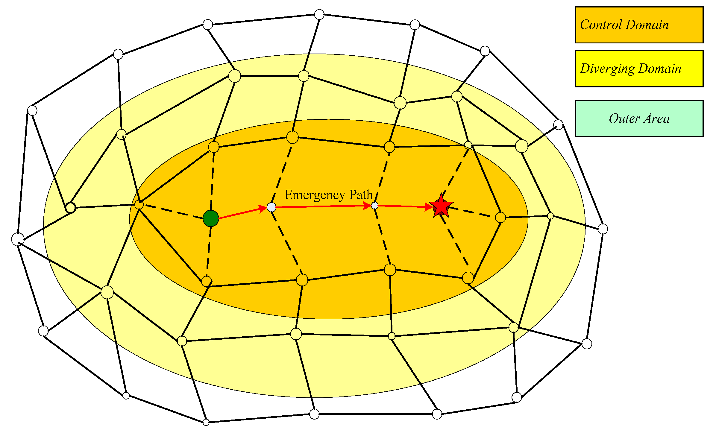
Control domain refers to the controlled emergency path as well as the network structure composed of road sections and nodes directly connected to the path. In Figure 1, the red nodes and sections make up the emergency path, and the road sections and nodes directly connected to the paths (the dotted line) which are directly affected by the control measures are also included in the control domain.
The outer area adjacent to the control domain is called the diverging domain, which is the main bypass area for social vehicles. This domain is defined by the basic bypass rules of the vehicles. Generally it is a network structure composed of road sections whose nodes are connected to the outer nodes of CD and the number of plies is not more than some integer. The area outside of the diverging domain is little affected by the controls and is usually not considered.
3.1.3. Control Node
Control node refers to the cross points within the regulation domain CD. As shown in Figure 1, the nodes in the inner ellipse are called control nodes. We use the quadruple group vnode: = <pos, CVB-SP, pd, de> to represent the control node, where pos means the nodal coordinate, CVB-SP means the vertex betweenness of the node [9], pd is the population density around the node, and de is the degree of the node. We know that a larger vertex betweenness implies more importance in the network. pd ranges from one to four, which represent small, normal, dense and very dense populations, respectively. When the pd is larger, the negative impact that a regulation has on society is larger. We define the importance of node i as follows:
In Equation (1), avg(pd) is the average population density of all of the nodes and max(pd) is the largest. In this equation we let and .
3.1.4. Control Type
Control type is used to restrict the permission of social vehicles to pass through the road section within the CD.
As shown in Figure 2, we designed three basic control types: non-control (N type), partial-control (P type) and all-control (A type) which are based on different regulation intensities. Partial control means that whereas emergency vehicles use the dedicated lanes, social vehicles can only use the rest of the lanes, to reduce the negative effects brought by the control strategy. In terms of the control intensity, the A type has the greatest influence on social vehicles, the P type takes second place and the N type is the least influential. Therefore, from the perspective of reducing the social impact, the A type should be restrictively used.
3.2. Problem Definition
Set as the urban road network (the outer area is not included). Let N be the set of all nodes and n be the number of nodes. Let L be the set of all directed edges (road sections) l be the number of edges. We suppose that all of the road sections are bidirectional and each road section can be described as lij which i,j N. Define node d as the disaster node, node o as the rescue node, and xo is the quantity of supplies that node o provides to node d. Based on the relevant description, graph G can be divided into two complementary sub-graphs: diverging domain and control domain CD. So we have , and . We make the following definitions.
: set of the TopN () shortest paths from rescue node o to disaster node d. These paths are called spare emergency paths, and means the kth alternative emergency path, where k = 0, 1, …, TopN − 1;
cIi,j: control intensity of road section , , ; value 0 represents non-control type, value 1 for all-control type and (0,1) for partial-control type;
eLk: set of all emergency sections in some emergency path k, , and k = 0, 1, …, TopN − 1;
: set of all road sections that are identified as the control type k in some emergency path, which means we have regulation style N, L, A and , k = 0, 1, …, TopN − 1, s = 0~2;
: set of all sections that social vehicles can drive in, , k = 0, 1, … , TopN − 1; the number of road sections in is M, M > 0;
: traffic flow of road section in normal situation, ;
: traffic flow of road section under control condition, ;
: traffic capacity of road section , ;
time needed to pass road section in normal situation, ;
: time needed for social vehicles to pass road section during the control period, which is decided by the control intensity of the road section cIi,j, ;
: time needed for emergency vehicles to pass the road section during the control period, ;
psychological impact factor of a control. This factor refers to the percentage of social vehicles circumambulating because of the control measures; ;
deltx: increased traffic flow on the emergency paths caused by emergency vehicles during a control;
MaxCT: maximum control time that social people can bear, ;
MaxTol: maximum tolerance degree that social people have during a traffic control period, .
3.3. Mathematical Model
The mathematical model of our problem is
s.t.
Formula (2) is the objective function to minimize the disturbance degree, which describes the degree by comparing the changes in the road impedance before and after a traffic control, and is the regulatory factor. Formula (3) is used to calculate the control time. This time consists of two parts, the first part is the time needed for vehicles to pass through the emergency path and the second part is the longest time to pass through all of the road sections of the emergency path. The reason we define the control time of road sections as the sum of the two parts is that the emergency paths need to be regulated in advance to ensure rescue vehicles can pass smoothly. Formula (4) ensures that the control time does not exceed the maximum control time MaxCT. Formula (5) defines the control intensity of the road section. For example, if loc equals 0.5 the control intensity equals 0.5.
4. Problem Formulation and Solution Algorithm
4.1. Heuristic Selection of the Control Type
The edge betweenness of road section is used to describe the importance of the section in a road network. A larger edge betweenness implies a more important road section [20]. When selecting the control type we need to fully consider the edge and vertex betweenness and its environmental characteristics. Based on the edge betweenness and Formula (1) we define the road section’s importance index as
In Equation (6), we have and . The larger the population density around the road section is, the greater the traffic flow it will take and the more important the road section will be. Important sections of road can have relatively looser control types, because although strict types are conducive to rescue vehicles passing through, they can negatively influence more social vehicles. When determining the control type of road sections, the characteristics of nodes in the control domain are first considered. According to whether the node is on the emergency path or not, we divide the nodes into normal nodes and emergency nodes. Generally, a normal node is not on the emergency path and need not undertake the task of passing through emergency vehicles, whereas emergency nodes are on the emergency path and undertake this task.
Based on the above classification we should follow these principles when selecting the control type as (i) when both nodes of one road section are emergency ones we are more likely to choose the partial-type or all-control type and (ii) emergency road sections in the control domain are more likely to be subject to the partial-type or all-control type, whereas non-emergency roads are more likely to have the non-control or partial-control type, and (iii) according to the roulette principle the smaller the sip value of the road section is, the more likely we select a strict control type, and vice versa.
4.2. Adjustment of the BPR Function
While executing traffic control, an urban traffic network’s structure will change greatly. These changes include (i) on all-control road sections emergency vehicles pass through at speeds approximately equal to free flow, but social vehicles cannot pass and (ii) on partial-control road sections, where emergency vehicles pass through at speeds approximately equal to free flow, social vehicles pass slowly, as for the capacity of the road section is smaller, and (iii) on non-control road sections within the emergency area, emergency vehicles and social vehicles drive together at low speed, and (iv) if the road section is within the diverging domain, the speed of social vehicles will also decrease because the road section may take extra bypass traffic flow.
In order to depict the change of time that social vehicles need to pass a road section before and after a control is implemented we adjust the BPR function under different situations according to the following steps.
- Step 1
- Calculate the total traffic flow that CD overflows to the diverging domain G′ according to the characteristics of the traffic control strategy;
- Step 2
- Calculate the attraction force of each node in G′ to the overflow of the traffic flow;
- Step 3
- Calculate the traffic flow change of the emergency and social vehicles on each road section in CD and G′ considering both the traffic flow increase that emergency vehicles bring and the psychological effects of the control strategy, then calculate the vehicles’ travel times on each road section.
4.2.1. Estimation of Spillover Traffic Flow
During the control period there are two reasons for the spillover of the traffic flow in CD: one is that the traffic control limit of the road section makes social vehicles bypass it, the other is that the rapid spread of the traffic control information affects people’s travel psychology, which leads them to detour actively. According to Equation (5), the traffic flow of the social vehicles’ passable road section is
Formula (7) shows that on the emergency path in CD, if road section lij is not being controlled (), social and emergency vehicles travel together. Obviously, emergency vehicles bring a traffic flow increase deltx, and some social vehicles choose to bypass the control because of the spread of the regulation information. Thus, the estimated traffic flow amount is . On the other hand, if road section lij is on non-emergency road sections in CD and is not controlled (), only social vehicles can pass through. Since these vehicles are affected by the regulation information, the estimated traffic flow amount after the regulation is . When partially controlling the road section () parts of the road section do not allow social vehicles to pass, which changes the road structure. In terms of the road impedance, we can equivalently assume that the traffic flow increased. Considering the control’s psychological impact, the estimated traffic flow amount after the regulation is . Obviously it takes social vehicles more time to go through the road section in this case.
Based on Equation (7), the traffic flow spillover of each road section in different situations can be calculated. When the traffic flow spillover of road section is ; when the traffic flow of spillover road section is ; and when the traffic flow spillover is because the road section forbids social vehicles from passing through. We define as the traffic flow spillover of road section , define OV as the total traffic flow spillover of CD, then we have
Because the diverging domain is able to attract the traffic flow spillover of the regulation domain, we still need to analyze the attractive ability of all of the nodes in the diverging domain.
4.2.2. Attraction Effect of Traffic Flow
Studies have shown that the gravitation field theory can be used to describe the dynamic mechanism of the network traffic flow [21]. Take a start node in the road network as an example: if a vehicle passes through the node while driving to a neighbor node, the neighbor node is attractive to the vehicle. The attraction power is relevant to the transmission capacity of the node (vertex betweenness), the road congestion degree and the physical distance between the nodes. We also know that those nodes that are not directly adjoined in the network also have an attraction power, which decreases as the number of layers between them increases.
After executing the control strategy, the social traffic flow within CD is squeezed into the diverging domain . Thus, attracts the traffic flow from CD. With an increase of the distance from node i in the influence is gradually lessening, as shown in Figure 3.
, , we define unidirectional attraction of node p to node q as follows:
In Equation (10), parameter is the traffic capacity of node p and where refers to the traffic capacity of road section <p, p’>. Parameters are the current traffic flows of the two nodes, and we have and . Nb(.) is a set of the node’s direct neighbors, parameters and are separately the length of the shortest path between node p and q and the relevant layers, respectively. If these two nodes are direct neighbors, we have . Formula (10) shows that the attraction of node p in area G′ to node q in area CD is in inverse proportion to their squared distance. The larger the current traffic flow of node p is, the smaller the attraction to q will be. Similarly, the larger the current traffic flow of node q is, the larger the attraction of node p to q will be. Parameter is the normalization factor that is used to adjust the values in (0,1) of
Based on Equation (10), we can correlate the attraction of node i in diverging domain G′ to the social vehicles in control domain CD:
The attraction capacity of node i has important effects on the traffic flow changes of the controlled road section. The greater the node attraction is, the more obvious the traffic flow change of the road section which is connected to the node will be. According to Equation (11) nodes in the diverging domain G′ will attract the total traffic flow spillover of CD in a certain proportion, and Therefore, based on the total traffic flow spillover OV to the diverging domain the change of the traffic flow at each node can be estimated. Then, the travel times over all of the road sections after the regulation can be obtained.
4.2.3. Adjustment of the BPR Function
In this paper we adjust the BPR function of the Federal Highway Administration by using attractive parameters. This function is taken as the travel time function of all of the road sections after the regulation has been imposed.
In Equation (12), parameters are called regression coefficients. Typically equals 0.15 and equals 4, and is the free flow driving time of . We will now discuss the emergency vehicles and social vehicles separately.
For emergency vehicles, there is
Formula (13) implies that emergency vehicles drive on a non-control road section together with social vehicles. Based on Equation (7), the traffic flow of is When emergency vehicles drive on a control road section exclusively they are not affected by the social vehicles and can drive at free flow speed. By substituting Equation (13) into Equation (3) the control time of the strategy can be obtained. Based on the place where there are, social vehicles can be divided into two styles as driving in control domain CD and driving in diverging domain G′.
- (i)
- In the control domain CD, , there isBased on Equation (7), we obtain
- (ii)
- In the diverging domain G′, because all of the nodes have an attraction to the traffic flow in control area CD, the traffic flow on will increase. Based on Equation (9) and Equation (11), we have
Parameter is the out-degree of node i. We consider bi-directional roads in this article, so we have . The effect of Equation (16) is to averagely distribute the traffic flow attracted to node i to its directly-connected road sections. By substituting Equation (16) into Equation (14), we have
By substituting Equations (15) and (17) into Equation (2), we would obtain the disturbance degree of the control strategy. After comparing the different control strategies the optimal one will be obtained.
4.3. Algorithm for PD-TCM
After executing a specific control strategy, the road network structure and traffic flow will change greatly in a short term which will have an adverse impact on travel activities. Therefore, considered scientifically, not only should the optimal control strategy be made and published, but the public bypass proposal based on the control strategy should be published at the same time to reduce the negative effects.
4.3.1. Solution to the Optimal Traffic Control Strategy
The solution to the problem is an iterative optimization process. Since the emergency path includes many road sections and each road section can have different control types, we have to face a combinatorial optimization problem. Inasmuch as the actual road network is huge and traditional algorithms cannot quickly solve our problem, this paper puts forward a novel traffic control strategy based on a genetic algorithm. The solution steps are as follows and the process is shown in Figure 4.
- Step 1
- Initialization: input the road network data and demand information for supplies in the disaster zone before starting the traffic control.
- Step 2
- Calculate the TopN shortest paths from the rescue node to the disaster node as an alternative emergency path; obtain the set ; build the alternative control domain set based on all of the emergency paths.
- Step 3
- According to the road network data, before any traffic controls are imposed, obtain the travel times of all of the road sections in normal conditions.
- Step 4
- Randomly select an alternative control domain from set CD, use the improved GA algorithm above to generate the control type of all of the road sections, and calculate the travel times of all of the road sections after the traffic control has been imposed; under the premise of satisfying all of the constraints of the emergency rescue, calculate the dissatisfaction degree of the social vehicles and the control time of the area; then iteratively obtain the local optimal control strategy of the current emergency area.
- Step 5
- Another control domain, repeatedly execute Step 4, and comparatively obtain the current optimal control strategy. After completing the calculation of all of the alternative control domains, compare and derive the optimal traffic control strategy to finish the process.
In the above steps, the selection of the control type of each road section is the key step because it directly determines whether the control strategy is good or not. In this paper we use a genetic algorithm to generate the road-control-type chromosomes and compare their adaptability. The specifics are as follows: use a binary number to encode the chromosome genes, where the number of binary digits is determined by the number of control types. For example, when the control types include the non-control type, 1/4 control type, 1/2 control type, 3/4 control type and all-control type, a three-digit binary number encoding is adopted (shown in Figure 5).
After producing the initial population, chromosomes can be chosen by the tournament algorithm. A uniform crossover operator and uniform mutation operator are used in the mutation process. When the iteration count exceeds the allowed maximum, the algorithm is terminated.
4.3.2. Bypass Strategy
According to the principle of the gravity field model part of the traffic flow will be diverted to closer road sections. Based on Equation (18) we calculate the bypassing index of the road section :
The larger is, the more diverging flow will take after the control is implemented. After calculating the bypassing index of all road sections in the diverging domain, the top road sections with larger are chosen as bypass road sections and compose the bypass strategy.
5. Computational Experiments and Analysis
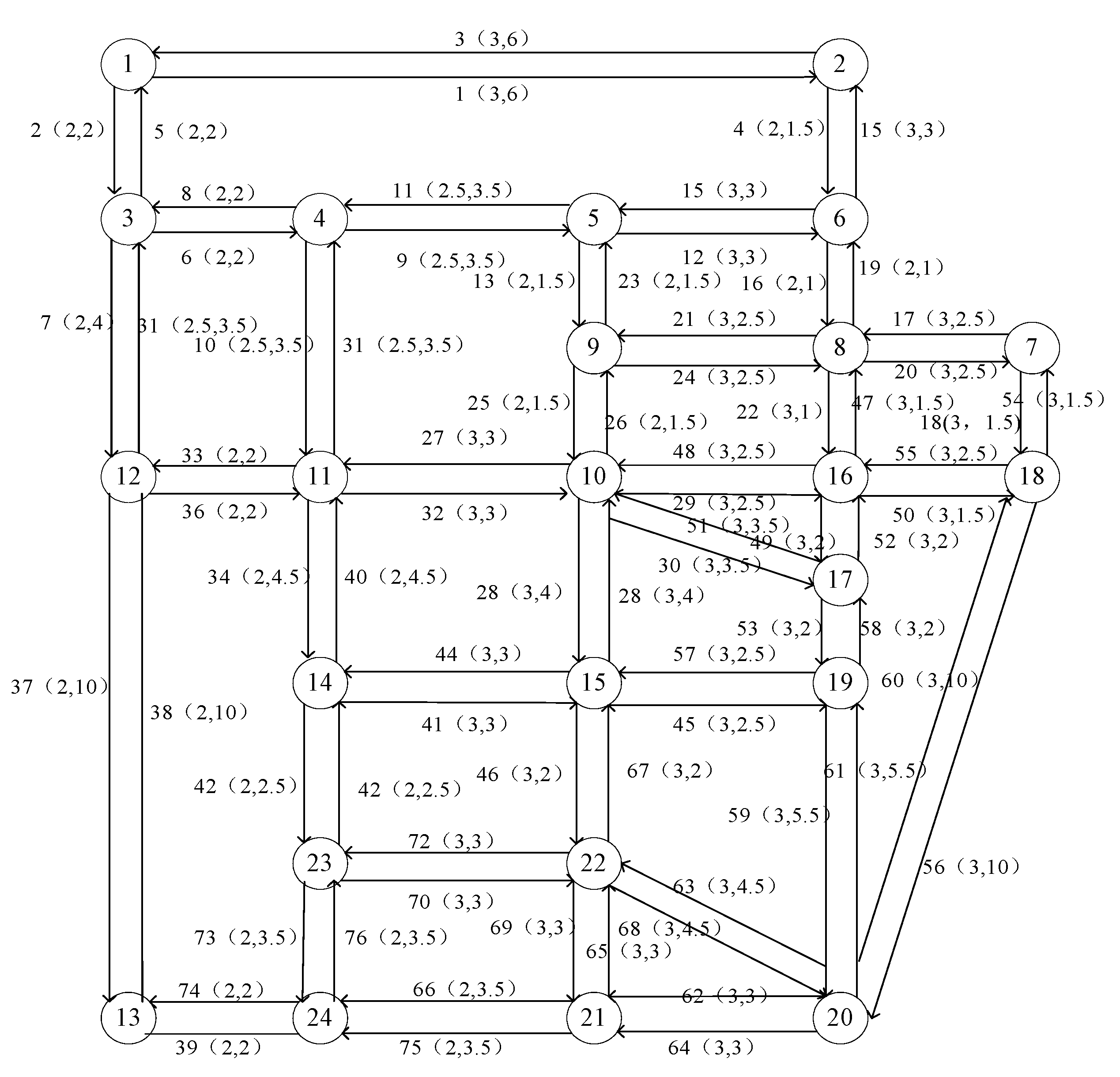
We take the Sioux-Fall road network in the American Northridge Earthquake in 1994 [22] and Flintbury City’s (a city in America) road network as examples. Sioux-Fall is a small network with 24 nodes and 76 road sections as shown in Figure 6. Flintbury is a large network with 1740 nodes and 2365 road sections (including bi-directional and one-way road sections). In this paper we mainly focus on the elaboration of the Sioux-Fall experiment, but we also present the results of the Flintbury experiment.
5.1. Sioux-Fall Experiment
5.1.1. Data and Parameters
In the Sioux-Fall network all road sections have been marked by number and capacity (unit: 5000 Vol/h, i.e., 5000 cars per hour) and driving time (h) in the format “road section number (capacity, driving time)”. The traffic flow, capacity and free flow times are shown in Table 1, the population density indexes of all of the nodes and the neighboring area are shown in Table 2, and the importance indices of all of the road sections calculated by Equation (6) are shown in Table 3. Let , , and
In the GA algorithm we use the tournament algorithm as the selection operator, select the uniform cross strategy as the cross operator, and use the uniform mutation strategy as the mutation operator. The population count is 20 and the maximum count of the iteration is no more than 1000.
5.1.2. Results and Analysis
• Experiment-1: Validity of the algorithm
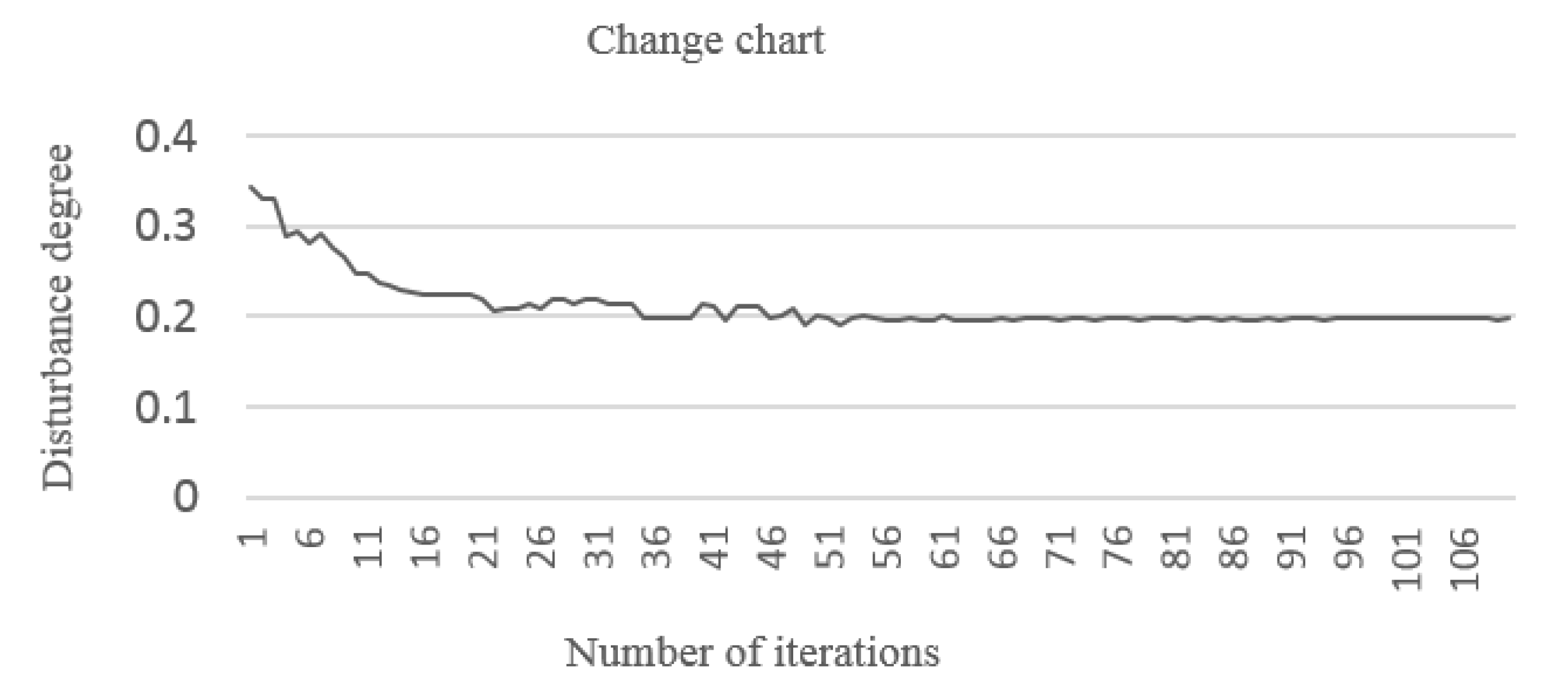
In this experiment, we suppose the rescue node is node 1 and the disaster node is node 20. The parameter TopN is set as five. In accordance with the requirements of the algorithm, the global optimal solution is the best control strategy of all of the types of control domains. Figure 7 shows the change of the objective function’s value with an increase or decrease in the number of iterations. We can conclude that as the number of iterations increases, the value of the objective function continuously decreases. In the early period, the value changes frequently because many bad chromosomes are present in the population. After 70 iterations, the system tends to be stable and reaches the optimum after approximately 400 iterations. Of course, there still exist individuals whose objective function value is lower than that of the optimal objective. Under the restrictions of the constraints these individuals will be eliminated.
The algorithm parameters and control strategy are shown in Table 4. The last column in the table shows the control types of the road sections on an emergency path. As the partial-control type increases, social vehicles can still drive on parts of road sections, and road utilization can be effectively guaranteed, which directly causes the traffic flow spillover in control areas and greatly reduces the disturbance degree. After 50 iterations, the current optimal strategy can be obtained: its disturbance degree is the smallest (0.19804), and the emergency vehicles’ traffic time (25.97675) also meets the demand. Without the partial-control type, excessive all-control types will seriously change the road network’s structure. As a result, the traffic flow will be greatly reduced and the traffic flow spillover will increase considerably. Thus, the diverging domain will receive an excessive traffic flow increase, which will seriously affect the traffic of social vehicles.
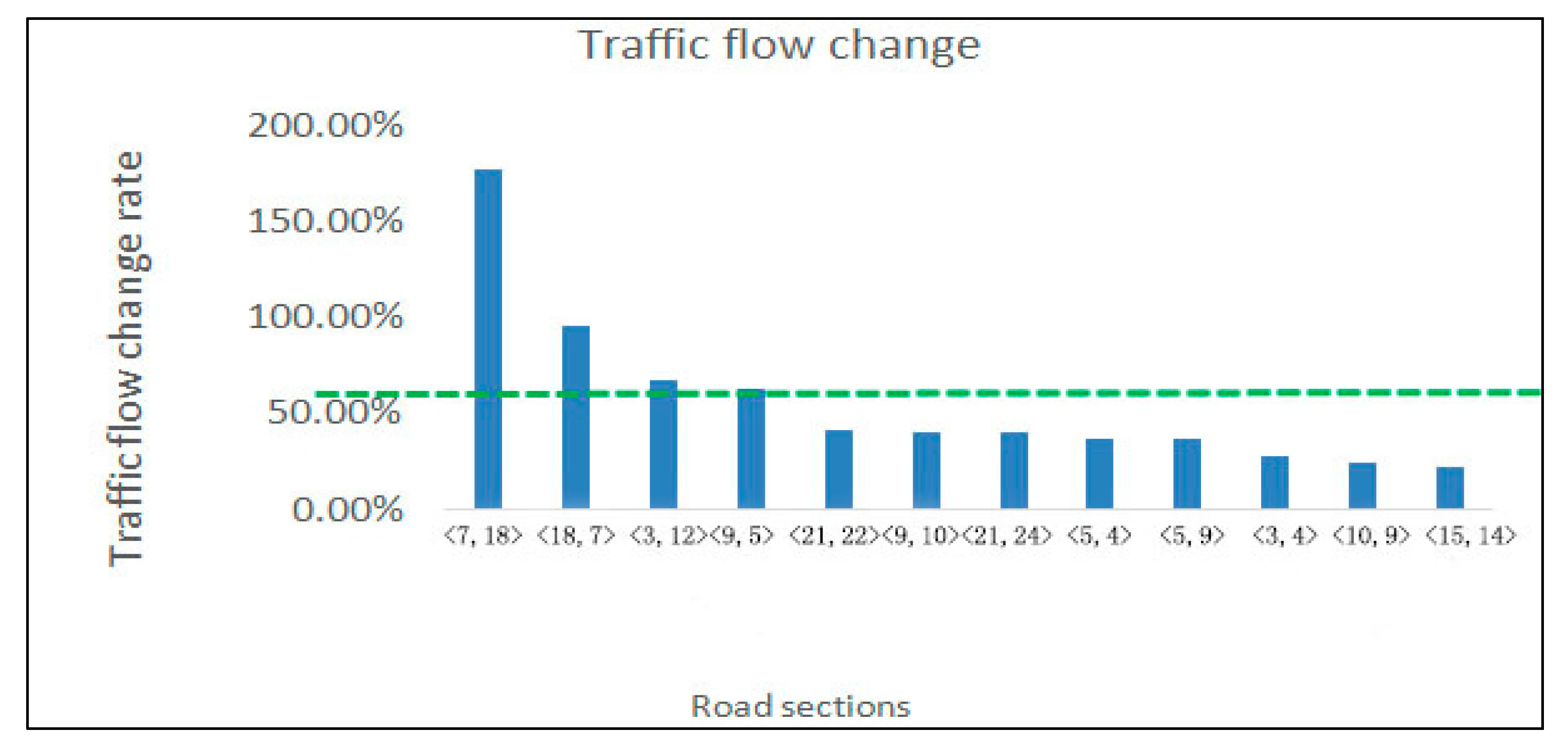
From Figure 8 we may find the change of traffic flow of road sections in the diverging domain after the regulation. The green dotted line represents the watershed of the change: in the upper part the change rate is larger than 50% and can even be greater than 150%. However, the change rate below the dotted line is small. When we are diverging the road section, we should focus on roads with larger change rates. Figure 9 shows the control domain, the diverging domain, the control types of all of road sections in the control domain, the traffic flow distribution (the numbers on the road sections), as well as the system’s recommended bypass road sections (marked in red).
As shown in the above figure, the change rates of road sections <7,18>, <18,7>, <3,12> and <9,5> are much larger. These rates demonstrate that the corresponding road sections can be used as bypass roads during a regulation, as shown in Figure 9.
• Experiment-2: Effect of control intensity
We set the psychological factor as 0.50, set the control intensity as 0.25, 0.50 and 0.75 in turn. We execute the algorithm again to obtain the results shown in Table 5.
If we refine the parameter value of the partial-control type, the disturbance degree of the regulation strategy can further decrease, which is consistent with actual situations. During the regulation period we cannot simply adopt the all-control type. We must properly reduce the control intensity based on the characteristics of the road sections, population density and related factors. Reducing the control intensity is beneficial to maintaining the connectivity and stability of the network structure, and more road resources are reserved to ensure the pass-through of social vehicles at the same time. In Table 5 we consider the all-control type as a special type of partial-control type (the control intensity equals 1.00). Although the control time is shorter, the disturbance degree is quite high. When only part of road sections are controlled the disturbance degree decreases greatly. Hence we can conclude that the smaller the control intensity is, the smaller the disturbance degree will be.
• Experiment-3: Effects of the psychological impact factor on the traffic flow
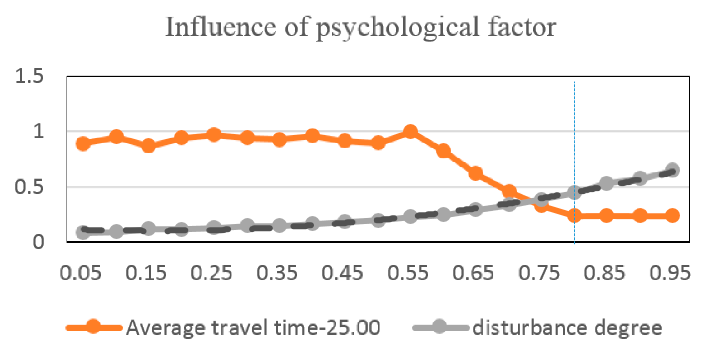
The promotion method and strength before starting the control and people’s social responsibility are reflected in the control strategy optimization process, as they are the effects of the psychological impact factor. When the other factors are unchanged, this experiment sets the intensity of the partial-control as 0.50, and the psychological factor takes values of 0.25–0.95 in turn. After repeating Experiment 1, we obtained the results shown in Table 6. As shown in the table, with the increase in the psychological factor, the disturbance degree increases and the average travel time of emergency vehicles decrease synchronously under fixed control intensity.
This conclusion is in line with our expectations and fits well with the actual situation. With the increasing publicity of traffic management departments, the ratio of social vehicles bypassing traffic control areas has gradually increased. More road resources are reserved for emergency vehicles, which results in lower average travel times for emergency vehicles and an increase in nuisance levels. However, the excessive publicity of traffic management is of little significance. In Figure 10, when the value of the psychological impact factor , is greater than 0.80, almost all social vehicles avoid the control region. Under this kind of situation on all control road sections, only emergency vehicles run at approximately free traffic flow and the values of control intensity of each road section in the control region is 1.00. At this point, the degree of disturbance will certainly continue to increase while the rescue efficiency of emergency vehicles has not been significantly improved. That is to say, when the psychological factor is large, the phenomenon of excessive waste of road resources appears, which is obviously not conducive to the efficient use of transportation resources and the implementation of equal rights for people to travel. Therefore, another area of concern in this paper is that traffic management departments should determine their propaganda based on the urgency of emergency rescue: when the level of urgency is high (for example, during the initial disaster relief) the government needs extensive publicity; and when the emergency level is not so high (for example, in the late period of disaster rescue) moderate publicity can be made to make full use of road resources. Generally, in practice, the application of any excessive or inadequate publicity is inappropriate.
5.2. Flintbury Experiment
This experiment takes the example of the actual road network structure of Flintbury City in the United States. Based on the principle of district division, the entire road network is divided into 12 districts (named TAZ, Traffic Analysis Zone), shown in Figure 11. When a disaster occurs in TAZ 6, supplies need to be transported to this area (shown in Figure 12). The red pentacle represents the disaster area and the green pentacle represents the rescue area. Supplies are transported from the rescue spot to the disaster spot, and the red solid line represents the alternative rescue route. The control domain is defined based on the rescue route, i.e., the yellow area. The remaining areas (5, 6, 7 and 8) are the diverging domain and the area outside of the diverging domain is the outer area.
Based on the road network structure characteristics of this experiment the control domain consists of emergency road sections, emergency nodes, and other road sections/nodes connected with them in two layers. The optimal regulation strategy is shown in Figure 13, in which the red road sections are under full control, blue sections are under partial control (control intensity equals 0.50) and green sections have no controls. Details of the control types of the road sections in the optimal schema are shown in Table 7.
The time constraint of the optimal control strategy is 8.50h. The rescue node of this strategy is No. 33438 and the disaster node is No. 51597. The emergency path of the optimal control schema is shown in Figure 14.
The sections that need to be bypassed are numbers 47083, 43891, 44432, 41776, 43081, 51962, 52066, 43027, 43046, 51476, 38769 and 38714. The experimental results show that our model is also effective for large-scale networks.
It needs to be explained that although Flintbury is a small city, the sections are relatively complex. Thus it is suitable to discuss the traffic control plan proposed by our research and these programs can also be mapped to large and medium-sized cities. The urban traffic management department will not block most roads in the process of material relief, but only control several key roads. After the implementation of traffic control, only some sections of the road around the road will be greatly affected. The greater the distance, the smaller the effect. Although the size of a city is related to the number of bars on the control road, the two are not linearly related. Of course, were we to find bigger or more representative cities, such as different topological structures of transportation networks and different scale cities, we would discuss our problems in more detail.
6. Suggestions and Discussion
Based on the data and experimental analysis, we obtained the following suggestions. (i) The government needs to establish and improve the real-time information release mechanism to ensure that the people can obtain real, effective and comprehensive information about the disaster in real time. Only by understanding the information regarding the disaster can people fully understand and support some traffic control measures. (ii) Through daily propaganda and training, ordinary people’s adaptability to emergency situations are gradually improved, so that they have the ability to help governments and social organizations by participating in rescue operations. Practice has proved that the power of the people is very huge and a well-trained population can play a great role in the rescue. The government can carry out community rescue based on people with professional rescue knowledge. (iii) It is vital to establish the whole process collection and analysis mechanism to accumulate data for disaster emergency rescue at a later time. Only by accumulating large amounts of historical data and using real-time data analysis and data mining tools for real-time analysis and command of the emergency rescue process, can we improve the efficiency and quality of a rescue process.
Our results can provide theoretical and technical support for decision-making departments to determine their post-disaster emergency decisions. However, there are still some problems in our research, such as (i) Our PD-TCM model has not considered the dynamic characteristics of road traffic flow, which probably makes the distribution of traffic somewhat stiff; (ii) the model has not considered some practical problems such as damage and emergency rehabilitation of road sections, which would cause a more complex situation; and (iii) when designing the control and diverging domain we did not consider the influence of the topological characteristics of road network.
7. Conclusions
A balanced temporary traffic control strategy can help meet the demands of the emergency rescue time and minimize the negative impact on society. The proposed PD-TCM model and relevant algorithms give full consideration to the optimization determination method of the emergency paths and control domain. To make full use of the road capacity and reduce the change in the network connectivity, a variety of control types with changeable control intensities are proposed, methods for the diverging domain to attract and distribute the traffic flow spillover from the control domain are used, and adjustments of the BPR function according to different road areas is improved. We also obtained the following management insights: (i) strengthen the daily information propaganda and constantly improve public awareness of the crisis and the authorities’ ability to respond to it. If people have enough coping capacity, the blindness of post-disaster traffic would significantly reduce; (ii) accelerate the construction of an emergency rescue linkage mechanism to ensure that the emergency management department and people can obtain enough real-time and correct information to avoid the adverse effects of information asymmetry; and (iii) conduct risk assessments, implement early warnings of the risk and develop emergency and rescue plans. Frequent emergency rescue drills should be carried out to improve the government and the public’s emergency response capability.
In the future, we will continue to carry out in-depth research into the dynamic characteristics of road traffic flow, damage and emergency rehabilitations of road sections and the influence of topological characteristics of road networks when disasters happens.
Acknowledgments
This work was supported by the National Natural Science Foundation of China (No. 70771094, 90924012, 71672154 and 71461027), the Humanities and Social Sciences Foundation of the Ministry of Education of China (No. 16YJA630038), the China Postdoctoral Science Foundation (No. 2016M592697), and the Key Science and Technology Project of Shandong Province in China (No. 2014GGH201022). The authors are grateful to the two anonymous reviewers for their constructive comments and invaluable contributions to enhance the presentation of this paper.
Author Contributions
Zengzhen Shao and Zujun Ma conceived and designed the experiments; Shulei Liu performed the experiments; Tongshuang Lv analyzed the data; Zengzhen Shao wrote the paper.
Conflicts of Interest
The authors declare that there is no conflict of interest regarding the publication of this paper.
References
- Kuroda, K.; Zhu, Q. Disaster damage and rehabilitation of urban transportation infrastructure. Urban Plan. Overseas 1996, 4, 11–15. [Google Scholar]
- Oh, N. Strategic uses of Lessons for Building Collaborative Emergency Management System: Comparative Analysis of Hurricane Katrina and Hurricane Gustav Response Systems. J. Homel. Secur. Emerg. Manag. 2012, 9. [Google Scholar] [CrossRef]
- Li, J.; Zhou, Y.; Liu, W. The Evaluation and Optimization of Post-earthquake Emergency Rescue Road Network in Shanghai Historic Area. J. Transp. Syst. Eng. Inf. Technol. 2017, 17, 227–233. [Google Scholar]
- Haddow, G.D.; Bullock, J.A.; Coppola, D.P. The Disciplines of Emergency Management: Preparedness. In Introduction to Emergency Management; Butterworth-Heinemann: Oxford, UK, 2017; pp. 121–158. [Google Scholar] [CrossRef]
- Kurauchi, F.; Iida, Y.; Shimada, H. Evaluation of road network reliability considering traffic regulation after a disaster. In The Network Reliability of Transport; Michael, G.H., Bell, Y.I., Eds.; Elsevier Ltd.: Oxford, UK, 2003; pp. 289–300. [Google Scholar] [CrossRef]
- Bauer, D.R.; Dickie, R.A. Simulation-based framework for transportation network management in emergencies. Transp. Res. Rec. 2008, 44, 80–88. [Google Scholar] [CrossRef]
- Faturechi, R.; Miller-Hooks, E. Measuring the performance of transportation infrastructure systems in disasters: A comprehensive review. J. Infrastruct. Syst. 2014, 21, 04014025. [Google Scholar] [CrossRef]
- Cui, J.X.; An, S.; Zhao, M. A generalized minimum cost flow model for multiple emergency flow routing. Math. Probl. Eng. 2014, 3, 1–12. [Google Scholar] [CrossRef]
- Papageorgiou, M.; Diakaki, C.; Dinopoulou, V.; Kotsialos, A.; Wang, Y. Review of road traffic control strategies. Proc. IEEE 2003, 91, 2043–2067. [Google Scholar] [CrossRef] [Green Version]
- Lee, C.-H. A Study on the Performance Meaning of Traffic Regulations on Road Section. Master’s Thesis, National Chiao Tung University, Hsinchu, Taiwan, 1998. [Google Scholar]
- Iida, Y.; Kurauchi, F.; Shimada, H. Traffic management system against major earthquakes. IATSS Res. 2000, 24, 6–17. [Google Scholar] [CrossRef]
- Oshima, D.; Tanaka, S.; Oguchi, T. Evaluation of traffic control policy in disaster case by using traffic simulation model. In Proceedings of the 19th ITS World Congress, Vienna, Austria, 22–26 October 2012; pp. 1–8. [Google Scholar]
- Shimada, H.; Iida, Y.; Kurauchi, F. Traffic regulation after an earthquake using ITS. In Proceedings of the 8th World Congress on Intelligent Transport Systems, Sydney, Australia, 30 September–4 October 2001. [Google Scholar]
- Yamada, A.; Takemoto, H.; Kobayashi, H.; Kuramoto, K.; Arakawa, M.; Nakayama, H.; Furukawa, K. A study on setting of standard rainfall for traffic regulation during heavy rainfall. J. Jpn. Soc. Eros. Control Eng. 2005, 57, 28–39. [Google Scholar] [CrossRef]
- Feng, C.-M.; Wen, C.-C. A fuzzy bi-level and multi-objective model to control traffic flow into the disaster area post-earthquake. J. East. Asia Soc. Transp. Stud. 2005, 6, 4253–4268. [Google Scholar]
- Wen, C.-C. Traffic Regulation Model Development and Application in Earthquake Disaster Area. Ph.D. Thesis, National Chiao Tung University, Hsinchu, Taiwan, 2006. [Google Scholar]
- Liu, H.X.; Ban, J.X.; Ma, W.; Mirchandani, P.B. Model reference adaptive control framework for real-time traffic management under emergency evacuation. J. Urban Plan. Dev. 2007, 133, 43–50. [Google Scholar] [CrossRef]
- Konstantinidou, M.A.; Kepaptsoglou, K.L.; Karlaftis, M.G.; Stathopoulos, A. Joint evacuation and emergency traffic management model with consideration of emergency response needs. Transp. Res. Rec. 2015, 2532, 107–117. [Google Scholar] [CrossRef]
- Chiou, Y.-C.; Lai, Y.-H. An integrated multi-objective model to determine the optimal rescue path and traffic controlled arcs for disaster relief operations under uncertainty environments. J. Adv. Transp. 2008, 42, 493–519. [Google Scholar] [CrossRef]
- Freeman, L.C. Centrality in social networks conceptual clarification. Soc. Netw. 2012, 1, 215–239. [Google Scholar] [CrossRef]
- Liu, G.; Li, Y.S.; Zhang, X.P. Analysis of network traffic flow dynamics based on gravitational field theory. Chin. Phys. B 2013, 22, 068901. [Google Scholar] [CrossRef]
- Chen, Y.W.; Tzeng, G.H. A fuzzy multi-objective model for reconstructing the post-quake road-network by genetic algorithm. Int. J. Fuzzy Syst. 1999, 1, 85–95. [Google Scholar]
Figure 1.
Sketch map of the urban network.

Figure 2.
Control types of a road section.
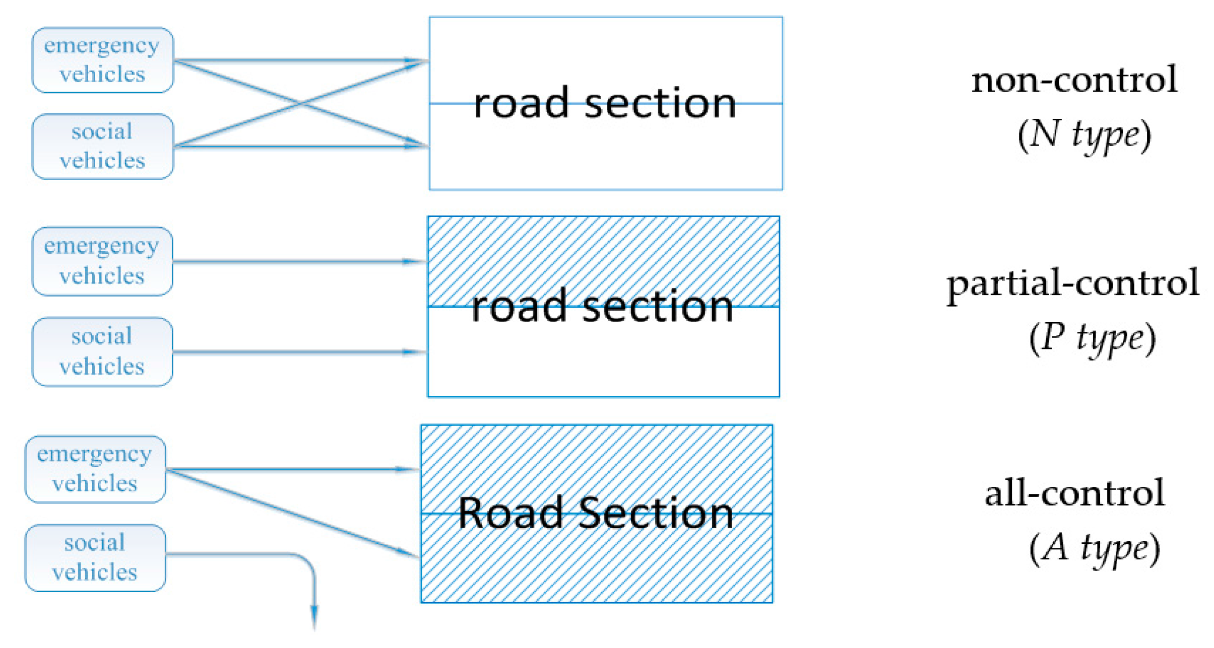
Figure 3.
Gravity model of the diverging domain.
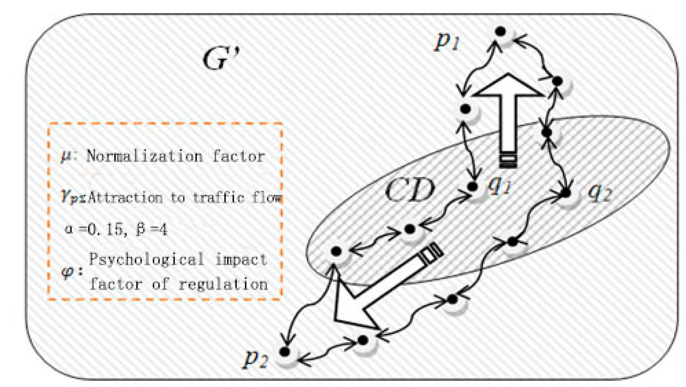
Figure 4.
Optimal selection process of the traffic control strategy.
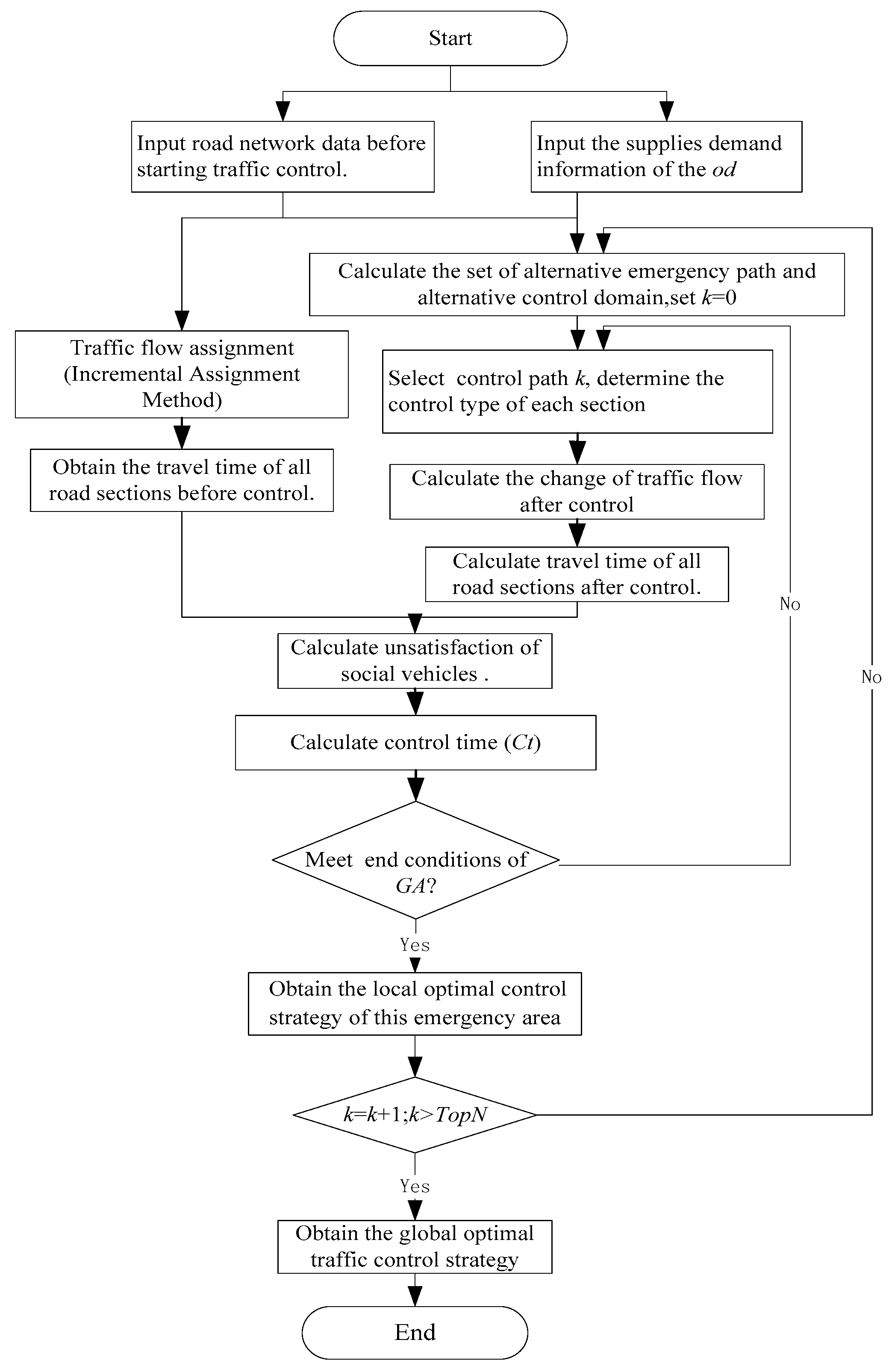
Figure 5.
Corresponding relations of the encoding mode and control type.
| Encoding mode | 000 | 001 | 010 | 011 | 100 |
| Control type | Non-control | 1/4 control | 1/2 control | 3/4 control | All-control |
| Control intensity | 0.00 | 0.25 | 0.50 | 0.75 | 1.00 |
Figure 6.
Sioux-Fall network.

Figure 7.
Changes in the objective value with iterations.

Figure 8.
Traffic flow change of road sections within the diverging domain.

Figure 9.
Optimal control strategy.

Figure 10.
Influence of psychological factors.

Figure 11.
TAZs and road network structure.

Figure 12.
Domain distribution.
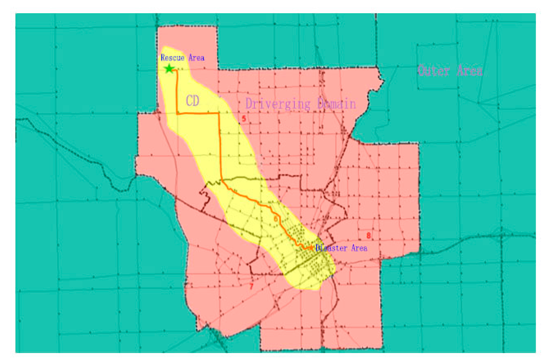
Figure 13.
Sketch of the optimal control strategy.

Figure 14.
Emergency path of the optimal control schema.
| 33438 → 34038 → 33430 → 32487 → 38150 → 38262 → 38182 → 18174 → 38190 → 38288 → 43480 → 43496 → 44082 → 44090 → 44122 → 44955 → 44923 → 44915 → 44931 → 44939 → 42868 → 42860 → 42876 → 42820 → 42828 → 43320 → 43312 → 42708 → 42700 → 42692 → 51621 → 51637 → 51597 |

Table 1.
Traffic flow, capacity and free flow time.
| Free Flow Time | Free Flow Time | Free Flow Time | |||||||||
|---|---|---|---|---|---|---|---|---|---|---|---|
| <1,2> | 3795 | 15,000 | 6 | <10,11> | 20,086 | 15,000 | 3 | <17,19> | 25323 | 15000 | 2 |
| <1,3> | 5997 | 10,000 | 2 | <10,15> | 20,506 | 15,000 | 4 | <18,7> | 12,344 | 15,000 | 1.5 |
| <2,1> | 3802 | 15,000 | 6 | <10,16> | 18,280 | 15,000 | 2.5 | <18,16> | 8179 | 15,000 | 2.5 |
| <2,6> | 6603 | 10,000 | 1.5 | <10,17> | 13,100 | 15,000 | 3.5 | <18,20> | 5949 | 15,000 | 10 |
| <3,1> | 5995 | 10,000 | 2 | <11,4> | 9503 | 12,500 | 3.5 | <19,15> | 11,181 | 15,000 | 2.5 |
| <3,4> | 8810 | 10,000 | 2 | <11,10> | 19,757 | 15,000 | 3 | <19,17> | 24,968 | 15,000 | 2 |
| <3,12> | 3595 | 10,000 | 4 | <11,12> | 13,675 | 10,000 | 2 | <19,20> | 10,747 | 15,000 | 5.5 |
| <4,3> | 8794 | 10,000 | 2 | <11,14> | 13,970 | 10,000 | 4.5 | <20,18> | 6157 | 15,000 | 10 |
| <4,5> | 9720 | 12,500 | 3.5 | <12,3> | 3608 | 10,000 | 4 | <20,19> | 10,630 | 15,000 | 5.5 |
| <4,11> | 9260 | 12,500 | 3.5 | <12,11> | 13,694 | 10,000 | 2 | <20,21> | 8295 | 15,000 | 3 |
| <5,4> | 9466 | 12,500 | 3.5 | <12,13> | 8369 | 10,000 | 10 | <20,22> | 6822 | 15,000 | 4.5 |
| <5,6> | 2700 | 15,000 | 3 | <13,12> | 8497 | 10,000 | 10 | <21,20> | 8191 | 15,000 | 3 |
| <5,9> | 9693 | 10,000 | 1.5 | <13,24> | 9013 | 10,000 | 2 | <21,22> | 8351 | 15,000 | 3 |
| <6,2> | 6605 | 10,000 | 1.5 | <14,11> | 14,065 | 10,000 | 4.5 | <21,24> | 8530 | 10,000 | 3.5 |
| <6,5> | 2569 | 15,000 | 3 | <14,15> | 13,685 | 15,000 | 3 | <22,15> | 21,847 | 15,000 | 2 |
| <6,8> | 11,111 | 10,000 | 1 | <14,23> | 12,390 | 10,000 | 2.5 | <22,20> | 6918 | 15,000 | 4.5 |
| <7,8> | 8710 | 15,000 | 2.5 | <15,10> | 20,626 | 15,000 | 4 | <22,21> | 8241 | 15,000 | 3 |
| <7,18> | 9747 | 15,000 | 1.5 | <15,14> | 13,905 | 15,000 | 3 | <22,23> | 13,245 | 15,000 | 3 |
| <8,6> | 10,980 | 10,000 | 1 | <15,19> | 10,941 | 15,000 | 2.5 | <23,14> | 12,266 | 10,000 | 2.5 |
| <8,7> | 6113 | 15,000 | 2.5 | <15,22> | 21,846 | 15,000 | 2 | <23,22> | 13,235 | 15,000 | 3 |
| <8,9> | 7311 | 15,000 | 2.5 | <16,8> | 17,398 | 15,000 | 1.5 | <23,24> | 5597 | 10,000 | 3.5 |
| <8,16> | 20,581 | 15,000 | 1 | <16,10> | 18,674 | 15,000 | 2.5 | <24,13> | 9041 | 10,000 | 2 |
| <9,5> | 9571 | 10,000 | 1.5 | <16,17> | 17,028 | 15,000 | 2 | <24,21> | 8535 | 10,000 | 3.5 |
| <9,8> | 7765 | 15,000 | 2.5 | <16,18> | 10,468 | 15,000 | 2.5 | <24,23> | 5468 | 10,000 | 3.5 |
| <9,10> | 14,830 | 10,000 | 1.5 | <17,10> | 13,243 | 15,000 | 3.5 | ||||
| <10,9> | 15,255 | 10,000 | 1.5 | <17,16> | 16,535 | 15,000 | 2 | ||||
Table 2.
Population density indexes among all of the nodes (pdi).
| i | pdi | i | pdi | i | pdi |
|---|---|---|---|---|---|
| 1 | 1 | 9 | 2 | 17 | 3 |
| 2 | 1 | 10 | 3 | 18 | 3 |
| 3 | 1 | 11 | 2 | 19 | 4 |
| 4 | 1 | 12 | 2 | 20 | 4 |
| 5 | 2 | 13 | 4 | 21 | 4 |
| 6 | 1 | 14 | 4 | 22 | 4 |
| 7 | 3 | 15 | 3 | 23 | 4 |
| 8 | 3 | 16 | 3 | 24 | 4 |
Table 3.
Betweenness and importance indexes of the road sections.
| <1,2> | 0.0181 | 5.5698 | <8,7> | 0.0326 | 25.22255 | <13,24> | 0.0344 | 7.64845 | <19,17> | 0.0507 | 12.8441 |
| <1,3> | 0.0272 | 5.5698 | <8,9> | 0.0109 | 38.9992 | <14,11> | 0.0217 | 22.0171 | <19,20> | 0.0127 | 7.6376 |
| <2,1> | 0.0181 | 3.56525 | <8,16> | 0.1232 | 42.66785 | <14,15> | 0.0272 | 35.23235 | <20,18> | 0.0145 | 4.026 |
| <2,6> | 0.0525 | 15.81875 | <9,5> | 0.0308 | 19.79665 | <14,23> | 0.0217 | 5.2421 | <20,19> | 0.0127 | 7.6376 |
| <3,1> | 0.0271 | 5.5698 | <9,8> | 0.0996 | 39.04355 | <15,10> | 0.1431 | 72.47785 | <20,21> | 0.0163 | 13.6394 |
| <3,4> | 0.0543 | 15.9834 | <9,10> | 0.0471 | 55.4173 | <15,14> | 0.0271 | 35.2323 | <20,22> | 0.0199 | 26.0412 |
| <3,12> | 0.0072 | 7.17235 | <10,9> | 0.1141 | 55.4508 | <15,19> | 0.0254 | 37.23145 | <21,20> | 0.0163 | 13.6394 |
| <4,3> | 0.0507 | 15.9816 | <10,11> | 0.0942 | 59.24085 | <15,22> | 0.1359 | 55.6867 | <21,22> | 0.0725 | 34.8675 |
| <4,5> | 0.0308 | 15.58415 | <10,15> | 0.1431 | 72.47785 | <16,8> | 0.0380 | 42.62525 | <21,24> | 0.0543 | 18.0584 |
| <4,11> | 0.0580 | 29.59775 | <10,16> | 0.0308 | 59.02165 | <16,10> | 0.1051 | 59.0588 | <22,15> | 0.1359 | 55.6867 |
| <5,4> | 0.0236 | 15.58055 | <10,17> | 0.0254 | 48.01895 | <16,17> | 0.0344 | 26.22345 | <22,20> | 0.0199 | 26.0412 |
| <5,6> | 0.0091 | 17.1733 | <11,4> | 0.0616 | 29.59955 | <16,18> | 0.0326 | 20.22255 | <22,21> | 0.0725 | 34.8675 |
| <5,9> | 0.0525 | 19.8075 | <11,10> | 0.0870 | 59.23725 | <17,10> | 0.0254 | 48.01895 | <22,23> | 0.0271 | 25.6448 |
| <6,2> | 0.0525 | 15.5825 | <11,12> | 0.0380 | 20.80025 | <17,16> | 0.0344 | 26.22345 | <23,14> | 0.0181 | 5.2403 |
| <6,5> | 0.0236 | 17.18055 | <11,14> | 0.0254 | 22.01895 | <17,19> | 0.0507 | 12.8441 | <23,22> | 0.0271 | 25.6448 |
| <6,8> | 0.0779 | 36.4202 | <12,3> | 0.0109 | 7.1742 | <18,7> | 0.0199 | 2.8162 | <23,24> | 0.0145 | 8.8385 |
| <7,8> | 0.0435 | 25.228 | <12,11> | 0.0380 | 20.80025 | <18,16> | 0.0217 | 20.2171 | <24,13> | 0.0380 | 7.65025 |
| <7,18> | 0.0091 | 2.8108 | <12,13> | 0.0109 | 2.0917 | <18,20> | 0.0145 | 4.026 | <24,21> | 0.0543 | 18.0584 |
| <8,6> | 0.0924 | 36.42745 | <13,12> | 0.0145 | 2.8135 | <19,15> | 0.0253 | 37.2314 | <24,23> | 0.0109 | 8.8367 |
Table 4.
Data collection from one experiment (using genetic algorithm) (MaxCT = 26, = 0.5, cI = 0.5, M0 = 1).
Table 4.
Data collection from one experiment (using genetic algorithm) (MaxCT = 26, = 0.5, cI = 0.5, M0 = 1).
| Iteration | Disturbance Degree (Optimal Value) | Travel Times of Emergency Vehicles | Control Types and Sections (All-Control: A; Partial-Control: P; Non-Control: N) |
|---|---|---|---|
| 10 | 0.24616 | 25.96461 | (A: <5,6>) (P: <1,2>, <6,8>, <7,8>, <9,8>, <16,7>, <21,20>, <22,20>) (N: others) |
| 20 | 0.21042 | 25.97137 | (A: none) (P: <2,6>, <6,8>,<8,16>) (N: others) |
| 30 | 0.20071 | 25.97675 | (A: none) (P: <1,2>, <5,6>, <6,8>, <19,20>) (N: others) |
| 40 | 0.20996 | 25.96262 | (A: none) (P: <1,2>, <3,1>, <16,17>, <19,20>) (N: others) |
| 50 | 0.19804 | 25.97675 | (A: none) (P: <1,2>, <6,8>, <19,20>) (N: others) |
Table 5.
Validity of the changeable control intensity of the partial-control type. (MaxCT = 26, = 0.5, = 0.5, M0 = 1).
Table 5.
Validity of the changeable control intensity of the partial-control type. (MaxCT = 26, = 0.5, = 0.5, M0 = 1).
| No. | Control Intensity (Partial-Control Type) | Average Disturbance Degree/Emergency Vehicles’ Average Travel Time |
|---|---|---|
| 1 | 0.25 (1/4 lanes under control) | 0.1849/25.84 |
| 2 | 0.50 (1/2 lanes under control) | 0.1980/25.98 |
| 3 | 0.75 (3/4 lanes under control) | 0.2109/25.98 |
| 4 | 1.00 (total regulation: all lanes under control) | 0.2434/25.99 |
| 5 | Mixed (include all control types) | 0.2215/25.99 |
Table 6.
Effects of changing the psychological factor. (MaxCT = 26, = 0.5, cI = 0.5, M0 = 1).
| No. | Psychological Factor | Avg. Disturbance Degree | Emergency Vehicles’ Avg. Travel Time |
|---|---|---|---|
| 1 | 0.95 | 0.6496 | 25.24 |
| 2 | 0.85 | 0.5327 | 25.24 |
| 3 | 0.80 | 0.4447 | 25.24 |
| 4 | 0.75 | 0.3878 | 25.33 |
| 5 | 0.50 | 0.1971 | 25.89 |
| 6 | 0.25 | 0.1249 | 25.97 |
Table 7.
Control types of road sections.
| Control Type | Road Sections |
|---|---|
| All-control | <41425,41465>, <41625,41617>, <42660,42652>, <41465,41489>, <38230,38214>, <38214,38206>, <41617,41625>, <42652,42692>, <51565,51597> |
| Partial-control (1/2) | <34038,33430>, <32479,32487>, <38262,38182>, <38246,38254>, <44024,44066>, <40497,41473>, <41633,42213>, <42660,42652>, <42117,42125>, <50924,51653>, <33422,32463>, <43456,43448>, <43448,43416>, <41393,39946>, <38262,38150>, <40751,40695>, <42261,42269>, <42269,42077>, <42253,42077>, <42077,42253>, <41609,41633>, <42213,42237>, <42700,42692>, <51621,51693>, <42652,42676>, <51597,51565>, <42197,50924>, <51653,50924>, <52250,50988>, <50988,50980>, <50980,50940>, <51677,52266> |
| Non-control | Others |
© 2017 by the authors. Licensee MDPI, Basel, Switzerland. This article is an open access article distributed under the terms and conditions of the Creative Commons Attribution (CC BY) license (http://creativecommons.org/licenses/by/4.0/).
Share and Cite
MDPI and ACS Style
Shao, Z.; Ma, Z.; Liu, S.; Lv, T. Optimization of a Traffic Control Scheme for a Post-Disaster Urban Road Network. Sustainability 2018, 10, 68. https://doi.org/10.3390/su10010068
AMA Style
Shao Z, Ma Z, Liu S, Lv T. Optimization of a Traffic Control Scheme for a Post-Disaster Urban Road Network. Sustainability. 2018; 10(1):68. https://doi.org/10.3390/su10010068
Chicago/Turabian StyleShao, Zengzhen, Zujun Ma, Shulei Liu, and Tongshuang Lv. 2018. "Optimization of a Traffic Control Scheme for a Post-Disaster Urban Road Network" Sustainability 10, no. 1: 68. https://doi.org/10.3390/su10010068
Note that from the first issue of 2016, this journal uses article numbers instead of page numbers. See further details here.