The Empirical Test on the Impact of Climate Volatility on Tourism Demand: A Case of Japanese Tourists Visiting Korea

1
Department of International Business and Trade, College of Politics and Economics KyungHee University, Seoul 02447, Korea
2
Research Department, The Bank of Korea, Seoul 04514, Korea
3
The International Trade Research Center at KyungHee University, Seoul 02447, Korea
*
Author to whom correspondence should be addressed.
Sustainability 2018, 10(10), 3569; https://doi.org/10.3390/su10103569
Submission received: 21 August 2018
/
Revised: 1 October 2018
/
Accepted: 1 October 2018
/
Published: 6 October 2018
(This article belongs to the Section Economic and Business Aspects of Sustainability)
Abstract
:As climate is not only a valuable tourism resource but also a factor influencing travel experience, estimating climate volatility has implications for sustainable development of the tourism industry. This study develops the Climate Volatility Index (CVI) using a Generalized Autoregressive Conditional Heteroscedasticity (GARCH) model and estimates the relationship between CVI and Japanese tourism demand in Korea, using a tourism demand model based on monthly data from January 2000 to December 2013. Possible time lags and multicollinearity among variables are considered for the model specification. The results show that an increase in climate volatility leads to a decrease in tourism demand.
1. Introduction
It is essential to respond properly to climate change for achieving sustainability of the tourism industry [1] because climate is a critical tourism resource as well as a determinant of tourist satisfaction, which affects tourism demand [2]. That is, climate change affects not only the destination attractiveness by inducing changes in tourism resources, but also the experience in traveling spots, which influences revisit intentions and potential customers [3]. Tourists can easily respond to climate change by changing their destination or vacation period. However, changes in tourism demand directly affect the economic outcome of those tourism destinations. Therefore, the understanding of the relationship between climate change and tourism demand is an important task for a sustainable development in the tourism industry in terms of economic aspects [4]. In particular, an accurate forecast of tourism demand is becoming more important for both efficient tourism operations and managerial decisions [2].
Many researchers have tried to identify the factors that affect tourism demand. Those factors include economic determinants such as income, tourism products, exchange rates, and non-economic determinants such as accessibility, environmental condition, cultural heritage, etc. The rapid climate change in recent years has brought about more studies on the relationship between climate and tourism demand [2,5]. Some studies have used individual climate factors such as the average or the extreme of precipitation and temperature to explain how these individual climate factors affect tourism demand [6,7]. Other studies have tried to explain the impact of climate change on tourism demand by using an index comprised of multiple indicators [8,9,10].
However, by taking both changing weather events and the degree of climate change, i.e., volatility, into consideration, the estimation of climatic impact can be more efficient and further improved. It is because climate is characterized by the distribution of frequencies, mean and extreme meteorological values [11] and the climate change of the past can affect that of the present as time series data are serially correlated to some extent [12]. The consideration of volatility also improves the accuracy of weather forecasts [13]. The volatility issue in climate change has been raised in Doods and Graci [14]. They concluded that the increased volatility and unpredictability combined with a warming trend in Canada would be a threat to its tourism industry.
The climate index, which takes volatility into account, can complement the existing indexes and present a more efficient approach to climate change. Cho [5] tried to reflect volatility by using the standard deviation of temperature. De Freitas, Scott, and McBoyle [15] pointed out that one of the limitations of the existing climate indexes is a heavy reliance on the mean value of climate indicators without conditioning variability or probability of key weather variables.
In this study, we tried to consider climate volatility explicitly in order to better explain the impact of climate change on tourism demand, aside from the average or the extreme of climate indicators. There are some studies that have attempted to estimate tourism demand with climate volatility considered, but more systematic approaches to volatility have not been sufficiently made so far.
There are many ways to identify the interrelationship between climate change and tourism demand, i.e., expert knowledge, statistical methods, survey, and observation [16]. This study seeks to estimate climate volatility using a Generalized Autoregressive Conditional Heteroscedasticity (hereafter, GARCH) model and verify the relationship between climate volatility and tourism demand. A GARCH model is useful in estimating the existence of time-dependent variance in climatic time series [7,8]. This study develops and applies two separate climate volatility indexes, one of which is the main GARCH Climate Volatility Index (hereafter, called mGCVI) based on precipitation, temperature, and snowfall, and the other one is the GARCH Climate Volatility Index (hereafter, called GCVI) based on precipitation, temperature, snowfall, sunshine, wind speed, insolation, and humidity. Since tourism demand can be affected not only by primary climate indicators such as precipitation, temperature, and snowfall but also by various other climate indicators, the application of mGCVI and GCVI in econometric estimation separately would help investigate more closely the relationship between climate volatility and tourism demand. This study also applies time-lags to the relationship between climate index and tourism demand by considering the decision-making process of tourists.
The analysis of this study is based on Japanese tourists to Korea. Japan is a geographically very close country and one of Korea’s largest tourism markets. Until 2012, the largest demand for tourism to Korea has come from Japan, and more than 2 million people have visited Korea every year [17]. Therefore, the analysis of the relationship between climate change in Korea and the demand of Japanese tourists for Korea is expected to provide important information on tourism supply and operations as well as the development of tourism policy in Korea.
The rest of this study is structured as follows: Section 2 presents theoretical backgrounds and previous studies on the relationship between climate change and tourism demand. Section 3 develops the climate volatility indexes and sets a model for analysis. Section 4 explains the results of analysis on the relationship between the climate volatility indexes and tourism demand based on the monthly data from January 2000 to December 2013. Section 5 summarizes the results with policy implications and suggests its limitations and directions for future studies.
2. Theoretical Background and Literature Review
2.1. Climate Change and Tourism Demand
Climate change is an important factor that can have a strong influence on tourism demand [1]. The environmental changes in tourism caused by climate change can affect not only tourists’ choice on where to visit but also their word-of-mouth intentions to revisit the destination through their tourism experience activities [9]. Previous studies on the relationship between climate change and tourism demand are categorized into those using individual climate indicators and others using an index based on multiple climate indicators. The studies that use individual climate indicators verified the impacts of climate change centering on temperature and precipitation. Specifically, Maddison [6] conducted a study on British tourists using temperature and precipitation as climate indicators and found that both temperature and precipitation have influences on tourism demand. In Maddison’s study, temperature shows a reversed-U shape, and the most preferred temperature is 30.7 °C, although the number of visits slightly declines at that point. Lise and Tol [7] carried out a study of the tourists from the OECD (The Organization for Economic Co-operation and Development) member countries and estimated the relationship between climate change and tourism demand by using temperature and precipitation as climate variables. The results confirm that both temperature and precipitation affect tourism demand. In their study, temperature also shows a reversed-U shape, and the most preferred temperature is 21 °C on average. According to a study of Chinese tourists to Korea conducted by Hwang et al. [18], a moderate increase in the average temperature positively affects tourism demand, and tourism demand is influenced by precipitation more than temperature when it comes to extreme weather events. In another study that used temperature as a climate indicator, Koenig and Abegg [19] argued that a 2 °C increase of temperature lowers the proportion of ski resorts in Switzerland down to 65 percent. The studies based on individual climate indicators are useful in estimating the direct influence of climate indicators but are considered short of estimating the overall impacts of climate change on tourists’ choice and behavior. This is because tourists perceive the climate differently from typical meteorological parameters and express their preference on climate by using several climate indicators combined [16]. For instance, when tourists are asked about the average daily temperature they prefer, they express their perception based on their cognitive information from past meteorological bulletins or cognitive reminding from their perception which combines humidity, wind, adaption, etc. [16]. Matzarakis [11] also concluded that a single parameter is inadequate for tourism climatology.
The research on the Tourism Climate Index (hereafter, TCI) is a good example that makes individual climate indicators into an index and verify its relationship with tourism demand. TCI, an index based on the climate environments of tourist destinations, standardizes and combines five climate indicators, such as daytime comfort index, day comfort index, precipitation, the duration of sunshine, and wind speed [20]. TCI ranges from −20 to 100, and the tourist destinations with a higher TCI represents better places for tourist activities. TCI is useful in figuring out how tourism demand in a specific region would evolve. By comparing Canada’s past TCI and future TCI based on the climate scenarios, Scott and McBoyle [10] predicted that tourism demand would increase in Western Canada and decrease in Eastern Canada. Through a TCI simulation, Amelung et al. [8] projected the changing patterns of tourism demand depending on climate change. Moore [5] looked into the Caribbean regions and drew a conclusion that the change in TCI has an influence on the attractiveness of tourism destinations, consequently affecting tourism demand.
TCI, however, has limitations in that each tourist has a different view of optimal climate conditions but an ‘expert-based’ index does not reflect the tourist’s preferences. Thus, no direct relationship is proven between climate change and tourism demand [9,15,21]. Morgan et al. [22] found there exits differences in the individual preferences of climate components, and Dubois et al. [23] concluded that TCI needs to better specify detailed data sources and its usage through a comparative study between Rutty and Scott [24] and Dubois et al. [25]. de Freitas, Scott, and McBoyle [15] developed an alternative to TCI, the Climate Index for Tourism (hereafter, CIT). CIT is a more efficient estimate of climate index that reflects tourists’ preferences, the relative importance of climate indicators, and key weather thresholds. However, it did not explicitly reflect the volatility of climate variables.
2.2. The Relationship between Climate Volatility and Tourism Demand
Climate is defined by the World Meteorological Organization as a statistical description in terms of mean and variability of relevant quantities over a period of time, namely 30 years [26]. It has a specific distribution of frequencies, mean, and standard deviation values [11]. Climate change refers to a statistically significant variation in either a mean value of climate or its variability persisting for an extended period [26]. Climate volatility refers to the second moment of distribution such as variance or standard deviation in the climate variability, which includes the first and the second moment of the climate data. This study adopts climate volatility instead of climate variability to focus on variance or standard deviation of the climate data in Korea. It is found that the time series of climate indicators frequently show conditional heteroscedasticity [12,27]. This means that the statistical characteristics of climate indicators need to be considered for an efficient estimation of climate change. For example, climate volatility of the past can affect that of the present [28]. Higher volatility means the variable changes more in magnitude and frequency [29,30].
Climate volatility affects tourism demand in two ways. First, tourism demand is affected through tourists’ expectations on travel destinations. Tourists choose travel destinations based on their expectations toward the region. These expectations are determined by tourists’ perception of the region, and one of the variables that affect their perception is the region’s climate [31,32]. In this process, an increase in climate volatility makes it difficult for tourists to predict this factor concerning travel destinations. To avoid heightened uncertainties, they may end up choosing alternative destinations with lower levels of climate volatility and uncertainties [33]. Thus, an increase in climate volatility can negatively affect tourism demand. Second, tourism demand is affected by the tourists’ own experience. Tourists’ experience is determined by their activities in travel destinations, and climate plays an important role in outdoor activities. For instance, people are usually disappointed when they experience continuous rainy days at their tourism destination during a vacation. In a study about the tourists to Scotland conducted by Smith [34], 20 percent of the visitors cited climate as the cause of their dissatisfactory travel experience. An increase in climate volatility implies tourists’ higher possibility of encountering unexpected climate events during their travel. Cho [5] also found that a large variation in temperature has a negative impact on tourism demand. Those unexpected climate events directly affect tourists’ satisfaction, and subsequently their reviews and willingness to revisit the region, thereby affecting tourism demand.
Another factor for consideration is a time-lag when we estimate the relationship between climate volatility and tourism demand. The choice of tourist destinations is the result of individual decision-making process. To choose where to visit, tourists collect various kinds of information and make plans based on the information they gathered [35]. Potential tourists choose a certain region when the gathered information says the region’s climate is suitable for traveling. On the other hand, when the information indicates unfavorable climate conditions for travel, they may choose other regions or adjust their travel schedule to avoid such weather events [7]. Thus, tourism demand in the present is formed based on the information that was gathered a certain time ago. According to a study conducted by Money and Crotts [36], Japanese tourists decide whether to travel 66 days prior to their departure date, while German tourists do so 131 days in advance. Also, Japanese tourists book flights 35 days prior to their departure, while German tourists do so 89 days in advance. What this implies is that climate volatility affects tourism demand with a certain time lag. Tourists do not distinguish at this point of time whether the expected inclement weather is due to a climate change or normal variability. However, as the increased climate volatility makes it more difficult for tourists to trust the weather information gathered for a destination decision, tourists may choose an alternative destination to avoid the risk [7].
Although some studies have attempted to verify the impact of the volatility of climate indicators on tourism demand, they are short of a more systematic approach to the estimation of volatility. Agnew and Palutikof [37] analyzed the impact of deviations from average temperature, precipitation, and sunshine on tourism demand in the Britain. The result confirms that an increase in precipitation negatively affects tourism demand, and that tourism demand is most sensitive to the volatility of climate indicators in March and April. Cin and Hwang [38] also carried out a study about Japanese tourists visiting Korea to find out the relationship between climate volatility and tourism demand by using daily average temperature and daily highest temperature. Their model shows that an increase in temperature boosts tourism demand among Japanese tourists to Korea, while volatility does not have the same effect.
This study applies a GARCH model to estimate and develop a climate volatility index. A GARCH model enables us to identify the second moments of variability of climate indicators and provides us with time-continuous series of GARCH variance that can be used to estimate the effect of climate volatility on the economic variables such as output or business activities. The model is also advantageous when it comes to the effect of extreme weather events on climate volatility.
2.3. Control Variables
In order to estimate the impact of climate volatility on tourism demand, this study sets income and travel cost as control variables based on previous studies. An increase in tourists’ income implies an increase in their purchasing power, which positively affects tourism demand. Most studies on tourism demand show that income is the most influential variable affecting tourism demand [39,40]. GDP, national income, disposable income and the index of industrial production are the main factors used in measuring tourists’ income. This study uses the monthly index of industrial production of Japan as a proxy variable for analysis. The index of industrial production, which measures industrial production activities during a certain period of time, tends to move along with the overall economic trend, so it is expected to reflect the overall changes in income. Another control variable is travel cost. An increase or decrease in travel cost would reduce or expand tourism demand. Travel cost is generally comprised of transportation costs and other expenses in tourist destinations. However, transportation cost is often excluded in recent studies on tourism demand due to a multicollinearity problem with income [41,42]. Thus, this study excludes transportation costs and includes other expenses in tourist destinations, by applying the ratio of Korea’s Consumer Price Index to that of Japan and adjusting exchange rates in the measurement. A relatively low travel cost in Korea implies that Japan’s Consumer Price Index is somewhat higher than that of Korea after adjusting for exchange rates.
3. Research Model
3.1. The Development of Climate Volatility Index
Based on previous studies, seven climate indicators that are expected to affect the tourism industry are chosen for the estimation of climate volatility index (CVI). The indicators are precipitation, temperature, wind speed, sunshine, snowfall, insolation, and humidity. Precipitation, temperature, and snowfall are core climate variables, and insolation, wind speed, sunshine, and humidity are the variables that are mainly included in the studies on tourists’ perception of climate. This study developed an index called mGCVI that consists of the three core climate indicators and another one called GCVI, consisting of all the seven indicators. An empirical study with theses indexes is expected to help figure out which type of volatility index is more closely related to the change of tourism demand. The operational definitions of each variable are as follows. The data used in this study is daily data observed for 24 h (every one hour) at 79 observation points nationwide, obtained from the national climate data center operated by Korea Meteorological Administration. These daily data were converted into monthly data. The period of analysis is 168 months, from January 2000 to December 2013.
We estimated a climate volatility index using an econometric method. First, we calculated the increase or decrease of each of the seven climate indicators, compared to the same month in the previous year for the period from 2000 to 2013. As Korea is known to have characteristically four seasons, we calculated the first differences from the same month in the previous year to overcome the seasonality issue, instead of applying a seasonal adjustment. Though this is not the best method to get rid of seasonality in time series, we can remove typical seasonal fluctuations and preserve the volatile characteristics of climate data in Korea by this alternative approach. Then we obtained the GARCH Variance of the first differences of each climate indicator by applying a GARCH model after removing discrepancies and outliers of data. The univariate GARCH (q,p) model applied for the estimation is as follows. The first formula is an average equation which has a constant term (c) and a standard error (εt). The second formula is a conditional variance equation, which is defined as ARCH () with a constant term (ω) and p lag of standard error and GARCH () which is a conditional variance of predicted error that has q lag. The value that refers to climate volatility is the GARCH Variance () that is estimated from this formula.
The results of volatility estimation under the GARCH model are shown in Table 1, which shows that all of the seven indicators have statistically significant volatility, i.e., GARCH Variance.
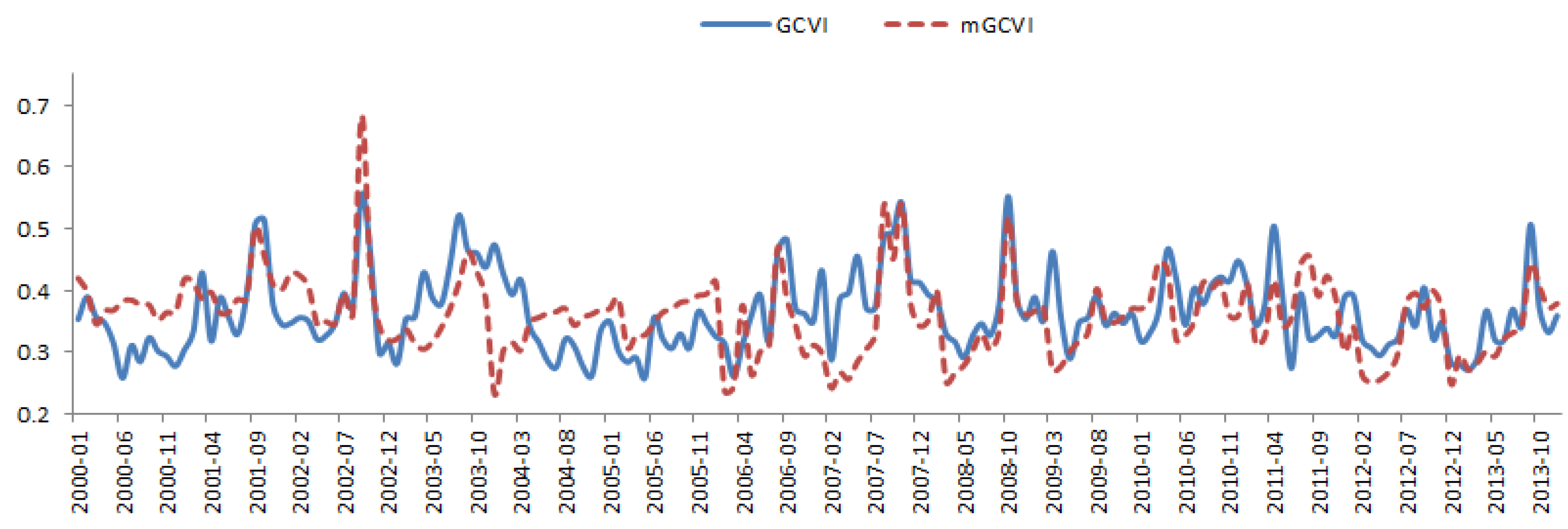
In order to develop a climate volatility index, each GARCH variance of the seven indicators was standardized to have values ranging from 0 to 1, and then we obtained two types of composite volatility indexes under the GARCH model by a linear combination of these variance. First, GCVI is a linear combination of the standardized GARCH variance of seven climate indicators. And mGCVI is a linear combination of the standardized GARCH variance of precipitation, temperature, and snowfall. Figure 1 is a graph showing the estimated GCVI and mGCVI during the analysis period. To check normality of the time series, the ADF (Augmented Dickey–Fuller) unit root test was performed, and the test results informed neither GCVI (t = −7.2462 ***) nor mGCVI (t = −7.5469 ***) has a unit root.
3.2. Tourism Demand Model
This study introduced a tourism demand model in order to verify the relationship between climate volatility and tourism demand as shown in the Equation (2). lnTAt refers to tourism demand and it is measured by a log transformation of the number of Japanese tourists visiting Korea at month t. lnINCOMEt refers to Japanese tourists’ income and it is measured by a log transformation of the income of Japanese tourists at time t. lnRECOSTt refers to the relative travel cost in Japan compared to that in Korea and it is measured by a log transformation of the relative travel cost at time t. And CVIt refers to the Climate Volatility Index of Korea at time t. All variables are monthly data.
lnTAt = α + δ1CVIt + β1lnINCOMEt + β2lnRECOSTt + εt
As tourism demand is expected to be autoregressive, and the past values of explanatory variables—tourist income, relative travel cost, and climate volatility—are also expected to affect tourism demand in the present, we modified the Equation (2) by applying an Autoregressive and Distributed Lags (ARDL) model as shown in the Equation (3). ARDL model is a dynamic model that reflects not only time lags of dependent variables but also multiple time lags of explanatory variables in regression equations [43]. The autocorrelation of error term of time series data can be significantly alleviated by this model, which leads to a more efficient estimation. Adding a time lag variable to the model provides better explanations thanks to the added information, however, it can also increase the size of distribution of the estimated variables and make current sample size insufficient for efficient estimation. Therefore, we applied the Akaike Information Criterion (AIC) to the model to determine the most appropriate time lags by considering the advantages and disadvantages of adding time lag variables.
lnTAt = α + γ1lnTAt−1+ ∙∙∙ + γp lnTAt−p + β1lnINCOMEt + ∙∙∙ + βqlnINCOMEt−q +
δ1lnRECOSTt + ∙∙∙ + δmlnRECOSTt−m + θ1CVIt + ∙∙∙ + θnCVIt−n + εt
δ1lnRECOSTt + ∙∙∙ + δmlnRECOSTt−m + θ1CVIt + ∙∙∙ + θnCVIt−n + εt
3.3. Data
The data used in this study are as follows. Daily climate observation data from January 2000 to December 2013 offered by the National Meteorological Office were transformed into monthly averages and used to estimate CVIs using a GARCH model. Tourism demand was measured as the number of Japanese nationals who visited Korea from January 2000 to December 2013, derived from monthly statistical data from the Korea Tourism Organization. Income was measured by the index of industrial production offered by Japan’s Ministry of Economy, Trade and Industry. The Consumer Price Index (2010 = 100) of Korea and Japan that were used to calculate the relative travel cost came from the data provided by the national statistical office of each country. Exchange rates are based on KRW/JPY rates from the Ministry of Strategy and Finance. The measurement of variables is shown in Table 2.
4. Results
4.1. Descriptive Statistics
The characteristics of descriptive statistics are shown in Table 3. The monthly average of lnTAt from January 2000 to December 2013 is 12.2618 with the lowest of 11.3292 and the highest of 12.7959. The standard deviation is 0.2303. The average of lnINCOMEt is 4.6249 with the lowest of 4.4987 and the highest of 4.7741. The standard deviation is 0.0513. The average of lnRECOSTt is 4.0167 with the lowest of 2.9648 and the highest of 4.8969. The standard deviation is 0.5131. The average of mGCVIt and GCVIt are 0.3805 and 0.3125 with the lowest of 0.1820 and 0.2076, and the highest of 0.6329 and 0.5053, respectively. The fluctuation of mGCVIt is greater than that of GCVIt.
4.2. Analysis Results
Prior to analyzing the relationship between climate volatility and tourism demand, a test was conducted to determine time lags by the Akaike Information Criteria (AIC), considering the autocorrelation of dependent and independent variables. According to the results of this test, we applied time lags for tourism demand ranging from t − 1 to t − 3 to minimize the value of AIC. For independent variables, i.e., lnINCOMEt, lnRECOSTt, and climate volatility indexes, we applied t for lnINCOMEt and t − 1 for lnRECOSTt, and t − 2 for mGCVIt, t − 3 for GCVIt, respectively. The summary of time lags of variables is shown in Table 4.
Based on these test results, we set our analysis model as follows. The Equation (4) intends to estimate the impact of mGCVIt, and the Equation (5) intends to estimate that of GCVIt on tourism demand.
lnTAt = α + γ1lnTAt−1 ∙∙∙ γ3 lnTAt−3 + β1lnINCOMEt + δ1lnRECOSTt + δ2lnRECOSTt−1 +
θ1mGCVIt + θ2mGCVIt−1 + θ3mGCVIt−2 + εt
θ1mGCVIt + θ2mGCVIt−1 + θ3mGCVIt−2 + εt
lnTAt = α + γ1lnTAt−1 + ∙∙∙ + γ3 lnTAt−3 + β1lnINCOMEt + δ1lnRECOSTt + δ2lnRECOSTt−1 +
θ1GCVIt + θ2GCVIt−1 + ∙∙∙ + θ4GCVIt−3 + εt
θ1GCVIt + θ2GCVIt−1 + ∙∙∙ + θ4GCVIt−3 + εt
We also conducted a multicollinearity diagnosis on the Equation (4). The variance inflation factor (VIF) of lnRECOSTt and lnRECOSTt−1 is over 10, which means there exists multicollinearity. So, we modified the Equation (4) by excluding lnRECOSTt−1. An autocorrelation test of error term was also conducted using the Breusch–Godfrey test, which proves the existence of the first-order autocorrelation in error term. By reflecting these test results, we excluded lnTAt−2 and lnTAt−3 and modified the Equation (4) into the Equation (6) to estimate the relationship between mGCVIt and tourism demand at t.
lnTAt = α + γ1lnTAt−1 + β1lnINCOMEt + δ1lnRECOSTt + θ1mGCVIt + ∙∙∙ + θ3mGCVIt−2 + εt
The adjusted R2 of the Equation (6) with mGCVIt is 65.53 percent, and the Durbin–Watson value is 1.91, which implies that the equation fits well without serial correlation. Looking more specifically at the analysis results, tourism demand shows no significant relationship with mGCVIt and mGCVIt−1, but shows a negative relationship with mGCVIt−2. lnTAt shows a positive relationship with lnTAt−1, lnINCOMEt and lnRECOSTt.
We then conducted a multicollinearity diagnosis on the Equation (5), and the result shows that VIF of lnRECOSTt and lnRECOSTt−1 is over 10. So, we excluded lnRECOSTt−1 from the Equation (5). Then, based on the Breusch–Godfrey test to detect an autocorrelation of error term, we excluded lnTAt−2 and lnTAt−3, and modified the Equations (5)–(7) to estimate the relationship between GCVIt and tourism demand at t.
lnTAt = α + γ1lnTAt−1 + β1lnINCOMEt + δ1lnRECOSTt + θ1GCVIt + ∙∙∙ + θ3GCVIt−2 + εt
The adjusted R2 of the Equation (7) with GCVIt is 64.58 percent, and the Durbin–Watson value is 1.83, which implies that the equation fits well and there is no autocorrelation. A closer look into the analysis results shows that there is no significant relationship between GCVIt and tourism demand at t. lnTAt shows a positive relationship with lnTAt−1, and both lnINCOMEt and lnRECOSTt show a positive relationship with lnTAt. While there shows a significant relationship between mGCVIt and tourism demand at t, we cannot find such a relationship between GCVIt and tourism demand at t. The estimation results of the Equations (6) and (7) are shown in Table 5.
5. Conclusions
5.1. Discussion and Implications
This study conducted an empirical analysis using monthly data from January 2000 to December 2013 in order to verify the impact of climate volatility on tourism demand. Based on the second moment of variability of climate indicators that was estimated using a GARCH model, we developed two climate volatility indexes to investigate their impacts on tourism demand. The first one is mGCVI that consists of precipitation, temperature, and snow fall. The second one is GCVI that consists of precipitation, temperature, wind speed, insolation, snow fall, sunshine, and humidity. We then set a regression model to analyze the impact of these climate volatility indexes on tourism demand, with lnTAt (tourism demand) as dependent variable, and lnINCOMEt (tourists’ income), lnRECOSTt (relative travel cost between Japan and Korea), climate volatility index as independent variables. We selected the appropriate time lags of each variable based on AIC, and set an Autoregressive and Distributed Lags model that includes t − 3 for lnTAt, t for lnINCOMEt, t − 1 for lnRECOSTt, t − 2 for mGCVIt, and t − 3 for GCVIt. We also excluded variables that exhibit multicollinearity and autocorrelation in error term.
Our empirical analysis shows that lnTAt−1, lnINCOMEt, lnRECOSTt all have a positive relationship with lnTAt. This means that an increase in Japanese tourists’ income leads to an increase in tourism demand for Korea, and an increase in relative travel cost in Japan also has the same effect, which confirms the results of previous studies [44,45]. The coefficients of lnINCOMEt measured by the industrial production index of Japan are 0.90 with mGCVIt and 0.82 with GCVIt variable, which are the largest among all the explanatory variables. This result does not deviate from our general conjecture that income is the most influential variable on tourism demand. It can be interpreted that one unit increase of income variable affects the tourism demand by 90 percent of one unit of the income variable, which is measured by the industrial production index of Japan. The coefficient of relative travel cost is 0.23 with 99 percent statistical significance when mGCVIt or GCVIt variable is included in the regression. That is, a unit change in the relative travel cost positively affects Japanese tourism demand for Korea by 23 percent of one unit of the relative travel cost variable. The 2017 International Visitor Survey by Ministry of Culture, Sports and Tourism supports these results. The Japanese tourism demand for Korea in the current period, lnTAt, also turns out to be strongly influenced by its own preceding variable, lnTAt−1.
The influence of the two types of climate volatility indexes, however, show different results. The mGCVIt shows a significantly negative relationship with tourism demand at t − 2. The coefficient of mGCVIt−2 is −0.42, which indicates a unit increase of climate volatility in terms of mGCVIt two months prior affects Japanese tourist demand for Korea by −42 percent of a unit mGCVIt−2. It means that the climate volatility in Korea in terms of mGCVIt two months prior negatively affects Japanese tourism demand for Korea in the current period. This result is consistent with the study of Money and Crotts [36], who argue that Japanese tourists generally make travel decisions two months prior to their departure. In Cho [5], a large temperature variation in a country showed a negative impact on the total tourist arrivals, although he did not consider applying a time-lag. This result implies that an increase in climate volatility in a certain area causes tourists to avoid traveling to that destination. A tourist response to climate change generally consists of adaptation, adjustment, and avoidance [46]. Tourists adapt themselves physiologically to some ranges of climate change. For instance, tourists are likely to visit as scheduled without taking any action if climate change at the destination is expected to be low. A low variation of climate change would not affect tourists’ satisfaction even during their visits, as they are physiologically adapted. Tourists try to adjust themselves to variations of climate change by preparing some items such as an umbrella for unexpected rainfall, clothes for unexpected cold, and an alternative tour program for unexpected weather, etc. However, if tourists are highly uncertain about the weather condition of travel destination when they plan, they may change their destination to a more suitable place or delay their travel schedule. His study confirms that Japanese tourists respond to climate volatility.
On the other hand, GCVIt shows no significant relationship with tourism demand at time t. We cautiously propose that this is attributable to the fact that Japanese tourists mostly visit large cities, and the relative importance of climate indicators that people actually perceive. While temperature and rainfall have direct impacts on tourists’ activities, humidity, insolation, sunshine, and wind speed have relatively less impacts on tourism. Another explanation might be that weather forecasts mainly focus on temperature and rainfall [35]. Since insolation, wind speed, sunshine, and humidity are not generally included in daily weather information, they rarely affect tourists’ decision making.
The theoretical implications of this study are as follows. Firstly, this study applies the concept of volatility to climate change. The explicit consideration of climate volatility in the analysis enables us to achieve a more efficient estimation by separately looking at the intrinsic changes and changes caused by distributional characteristics. Even though climate indicators show heteroskedasticity over time, they have only been discussed in a limited manner in the existing studies so far. By using a GARCH model, this study reflects non-linear characteristics of climate indicators as time series [47]. Secondly, this study developed and verified a new index representing the volatility of climate change. While TCI [20] and CIT [15] are useful in the evaluation of the climate environment of tourist destinations, those are limited in providing explanations for changes in tourism demand caused by climate change [9,21]. Individual climate indicators also have limitations as they cannot reflect the fact that tourists’ perception of climate is influenced by various climate factors. CVI suggested in this study consists of multiple climate indicators and presents climate volatility in the form of an index. If used together with TCI, CIT, and individual climate indicators when estimating the relationship between climate change and tourism demand, CVI could provide a more comprehensive understanding of the relationship by addressing the limitations of existing studies.
The managerial implications of this study are as follows. First, tourism services need to take climate volatility into account, as an increase in climate volatility leads to a decrease in tourism demand. Specifically, climate volatility can undermine the attractiveness of tourist destinations and tourists’ satisfaction, thereby negatively affecting tourism demand [48]. Therefore, providers in the tourism industry should consider, not only the average or extreme climate events, but also the volatility of climate indicators when discussing how to respond to climate change. For example, tourism service providers could reduce the influence of climate change on tourism attractiveness by expanding indoor tourist activities and infrastructures. Also, the tourism industry could develop tourism services that can address unexpected inconveniences caused by climate volatility, by providing tourists with major alternative tourist attractions and facilities. Adding a climate-related item to the International Visitor Survey, annually conducted by Ministry of Culture, Sports and Tourism, could help tourism service providers closely monitor the changes in the perception and attitudes of foreign tourists. By reflecting these results into their services, those providers will be able to respond more efficiently to the changes in tourism demand due to climate volatility. Second, the empirical results show that economic factors are still more important in the demand of Japanese tourists for visiting Korea. This means that the development of a price-competitive tourism product and services are most important in the Korean tourism industry. Finally, this study can be utilized to make decisions about the timing of marketing campaigns. To minimize the negative impact of climate volatility on tourism demand, the marketing activities for target tourists need to be implemented two months prior for successful marketing.
5.2. Limitations and Further Research
The limitations of this study are as follows. This study uses various climate variables that are expected to affect tourists’ decisions such as wind speed, insolation, sunshine, and humidity, but fails to consider tourists’ direct perception about climate volatility. According to previous studies there are some destinations that are chosen despite bad weather, even though climate is an important factor in deciding tourist destinations [32]. Therefore, it is important to develop how to capture the perception of tourists more precisely. This study is also limited in reflecting various control variables that affect tourism demand. In particular, a comparative analysis of tour regions needs to be considered, because an emergence of an attractive tourist destination may undermine tourism demand for neighboring regions [42]. Therefore, future studies should consider the relationship between climate volatility and tourism demand, together with tourists’ perspective and competing tourist destinations. Another possible topic would be the relationship between tourism demand and climate volatility projection, based on climate change scenarios such as the ENSEMBLES database generated by an EU-funded integrated project to develop an ensemble prediction system for climate change. This is expected to make it possible to predict the uncertainty of tourism demand together with other climate indexes.
Author Contributions
Y.S.H. and H.S.H.K. conceived and designed the research; H.S.H.K. and C.Y. analyzed the data; Y.S.H., C.Y., and H.S.H.K. wrote the paper
Funding
This work was supported by the Ministry of Education of the Republic of Korea and the National Research Foundation of Korea (NRF-2016S1A5B6925462).
Conflicts of Interest
The authors declare no conflict of interest.
References
- UNWTO; UNEP; WMO. Climate Change and Tourism: Responding to Global Challenges; UNWTO: Madrid, Spain, 2008. [Google Scholar]
- Goh, C. Exploring impact of climate on tourism demand. Ann. Tourism Res 2012, 39, 1859–1883. [Google Scholar] [CrossRef]
- Gössling, S.; Scott, D.; Hall, C.M.; Ceron, J.P.; Dubois, G. Consumer behaviour and demand response of tourists to climate change. Ann. Tourism Res 2012, 39, 36–58. [Google Scholar]
- Scott, D.; Jones, B.; Konopek, J. Exploring the impact of climate-induced environmental changes on future visitation to Canada’s Rocky Mountain National Parks. Tourism Rev. Int. 2008, 12, 43–56. [Google Scholar] [CrossRef]
- Cho, V. A study of the non-economic determinants in tourism demand. Int. J. Tourism Res. 2010, 12, 307–320. [Google Scholar] [CrossRef]
- Maddison, D. In search of warmer climates? The impact of climate change on flows of British tourists. Clim. Chang. 2001, 49, 193–208. [Google Scholar] [CrossRef]
- Lise, W.; Tol, R.S. Impact of climate on tourist demand. Clim. Chang. 2002, 55, 429–449. [Google Scholar] [CrossRef]
- Amelung, B.; Nicholls, S.; Viner, D. Implications of global climate change for tourism flows and seasonality. J. Travel Res. 2007, 45, 285–296. [Google Scholar] [CrossRef]
- Moore, W.R. The impact of climate change on Caribbean tourism demand. Curr. Issues Tourism 2010, 13, 495–505. [Google Scholar] [CrossRef] [Green Version]
- Scott, D.; McBoyle, G. Using a ‘tourism climate index’ to examine the implications of climate change for climate as a tourism resource. In Proceedings of the First International Workshop on Climate, Tourism and Recreation, Freiburg, Germany, 5–10 October 2001; pp. 69–88. [Google Scholar]
- Matzarakis, A. Weather-and climate-related information for tourism. Tourism Hosp. Plan. Dev. 2006, 3, 99–115. [Google Scholar] [CrossRef]
- Tol, R.S. Autoregressive conditional heteroscedasticity in daily temperature measurements. Environmetrics 1996, 7, 67–75. [Google Scholar] [CrossRef]
- Stern, H. Employing weather derivatives to assess the economic value of high-impact weather forecasts out to ten days–indicating a commercial application. In Proceedings of the 22nd Conference on Weather Analysis and Forecasting, Park City, UT, USA, 25–29 June 2007. [Google Scholar]
- Dodds, R.; Graci, S. Canada’s tourism Industry—Mitigating the effects of climate change: A lot of concern but little action. Tourism Hosp. Plan. Dev. 2009, 6, 39–51. [Google Scholar] [CrossRef]
- De Freitas, C.R.; Scott, D.; McBoyle, G. A second generation climate index for tourism (CIT): specification and verification. Int. J. Biometeorol. 2008, 52, 399–407. [Google Scholar] [CrossRef] [PubMed]
- Dubois, G.; Ceron, J.P.; Gössling, S.; Hall, C.M. Weather preferences of French tourists: Lessons for climate change impact assessment. Clim. Chang. 2016, 136, 339–351. [Google Scholar] [CrossRef]
- The Korea Tourism Knowledge & Information System. Available online: www.tour.go.kr (accessed on 8 August 2017).
- Hwang, Y.S.; Lee, Y.; Shim, C.; Choi, Y.J. Climate Change Impacts on Tourism Management in Korea. Korean Corp. Manag. Rev. 2014, 21, 57–70. [Google Scholar]
- Koenig, U.; Abegg, B. Impacts of climate change on winter tourism in the Swiss Alps. J. Sustain. Tourism 1997, 5, 46–58. [Google Scholar] [CrossRef]
- Mieczkowski, Z. The tourism climatic index: A method of evaluating world climates for tourism. Can. Geogr. 1985, 29, 220–233. [Google Scholar] [CrossRef]
- Scott, D.; Jones, B.; Konopek, J. Implications of climate and environmental change for nature-based tourism in the Canadian Rocky Mountains: A case study of Waterton Lakes National Park. Tourism Manag. 2007, 28, 570–579. [Google Scholar] [CrossRef]
- Morgan, R.; Gatell, E.; Junyent, R.; Micallef, A.; Özhan, E.; Williams, A.T. An improved user-based beach climate index. J. Coast. Conserv. 2000, 6, 41–50. [Google Scholar] [CrossRef] [Green Version]
- Dubois, G.; Ceron, J.P.; Dubois, C.; Frias, M.D.; Herrera, S. Reliability and usability of tourism climate indices. Earth Perspect. 2016, 3, 2. [Google Scholar] [CrossRef]
- Rutty, M.; Scott, D. Will the Mediterranean become “too hot” for tourism? A reassessment. Tourism Hosp. Plan. Dev. 2010, 7, 267–281. [Google Scholar] [CrossRef]
- Dubois, G.; Ceron, J.P.; van de Walle, I.; Martin, O.; Picard, R. Météorologie, Climat et Déplacements Touristiques: Comportements et Stratégies des Tourists; CREDOC: Paris, France, 2009. [Google Scholar]
- Glickman, T.S.; Zenk, W. Glossary of Meteorology, 2nd ed.; American Meteorological Society: Boston, MA, USA, 2000. [Google Scholar]
- Romilly, P. Time series modelling of global mean temperature for managerial decision-making. J. Environ. Manag. 2005, 76, 61–70. [Google Scholar] [CrossRef] [PubMed]
- Wang, W.; Van Gelder, P.H.A.J.M.; Vrijling, J.K.; Ma, J. Testing and modelling autoregressive conditional heteroskedasticity of streamflow processes. Nonlinear Process. Geophys. 2005, 12, 55–66. [Google Scholar] [CrossRef] [Green Version]
- Mantegna, R.; Stanley, H.E. An Introduction to Econophysics: Correlations and complexity in Finance; Cambridge University Press: Cambridge, MA, USA, 2000. [Google Scholar]
- Liu, Y.; Gopikrishnan, P.; Stanley, H.E. Statistical properties of the volatility of price fluctuations. Phys. Rev. E 1999, 60, 1390–1400. [Google Scholar] [CrossRef] [Green Version]
- Gallarza, M.G.; Saura, I.G.; Garcia, H.C. Destination image: Towards a conceptual framework. Ann. Tourism Res. 2002, 29, 56–78. [Google Scholar] [CrossRef]
- Gossling, S.; Bredberg, M.; Randow, A.; Sandström, E.; Svensson, P. Tourist perceptions of climate change: A study of international tourists in Zanzibar. Curr. Issues Tourism 2006, 9, 419–435. [Google Scholar] [CrossRef]
- Kahneman, D.; Tversky, A. Prospect theory: An analysis of decision under risk. Econometrica 1979, 47, 263–291. [Google Scholar] [CrossRef]
- Smith, K. The influence of weather and climate on recreation and tourism. Weather 1993, 48, 398–404. [Google Scholar] [CrossRef]
- Hamilton, J.M.; Lau, M.A. The role of climate information in tourist destination choice decision making. In Tourism and Global Environmental Change: Ecological, Economic, Social and Political Interrelationships, 1st ed.; Gossling, S., Hall., M., Eds.; Routledge: New York, NY, USA, 2006. [Google Scholar]
- Money, R.B.; Crotts, J.C. The effect of uncertainty avoidance on information search, planning, and purchases of international travel vacations. Tourism Manag. 2003, 24, 191–202. [Google Scholar] [CrossRef]
- Agnew, M.D.; Palutikof, J.P. Impacts of short-term climate variability in the UK on demand for domestic and international tourism. Clim. Res. 2006, 31, 109–120. [Google Scholar] [CrossRef] [Green Version]
- Cin, B.C.; Hwang, Y.S. An Analysis on Effects of Climate Changes on Japanese Tourism Demand for Korea. J. Korea Trade 2013, 38, 179–204. [Google Scholar]
- Webber, A.G. Exchange rate volatility and cointegration in tourism demand. J. Travel Res. 2001, 39, 398–405. [Google Scholar] [CrossRef]
- Uysal, M.; Crompton, J.L. Determinants of demand for international tourist flows to Turkey. Tourism Manag. 1984, 5, 288–297. [Google Scholar] [CrossRef]
- Li, G.; Song, H.; Witt, S.F. Recent developments in econometric modeling and forecasting. J. Travel Res. 2005, 44, 82–99. [Google Scholar] [CrossRef] [Green Version]
- Lee, C.G.; Song, G.S.; Song, H.J. Determinants of Bi-national Tourism Demand from Japan to Korea: Using Econometric Models. J. Tourism Leis. Res. 2006, 18, 7–25. [Google Scholar]
- Lim, C.; Zhu, L. Dynamic heterogeneous panel data analysis of tourism demand for Singapore. J. Travel Tourism Mark. 2017, 34, 1224–1234. [Google Scholar] [CrossRef]
- Dritsakis, N. Tourism as a long-run economic growth factor: an empirical investigation for Greece using causality analysis. Tourism Econ. 2004, 10, 305–316. [Google Scholar] [CrossRef]
- Daniel, A.C.M.; Ramos, F.F. Modelling inbound international tourism demand to Portugal. Int. J. Tourism Res. 2002, 4, 193–209. [Google Scholar] [CrossRef]
- Sonnenfeld, J. Variable values in space and landscape: An inquiry into the nature of environmental necessity. J. Soc. Issues 1996, 22, 71–82. [Google Scholar] [CrossRef]
- Modarres, R.; Ouarda, T.B.M.J. Generalized autoregressive conditional heteroscedasticity modelling of hydrologic time series. Hydrol. Process. 2013, 27, 3174–3191. [Google Scholar]
- Scott, D.; Lemieux, C. Weather and climate information for tourism. Procedia Environ. Sci. 2010, 1, 146–183. [Google Scholar] [CrossRef]
Figure 1.
Estimated Climate Volatility Indexes. Source: Author’s own elaboration.


Table 1.
Results of Volatility Estimation by Generalized Autoregressive Conditional Heteroscedasticity (GARCH).
Table 1.
Results of Volatility Estimation by Generalized Autoregressive Conditional Heteroscedasticity (GARCH).
| Indicator | Precipitation | Temperature | Wind Speed | Insolation | Snowfall | Sunshine | Humidity |
|---|---|---|---|---|---|---|---|
| ARCH(−1)2 | 0.4120 ** (0.0777) | −0.0103 (0.0170) | 0.0946 (0.1176) | 0.2769 ** (0.1052) | 0.5292 ** (0.0754) | 0.1379 * (0.0703) | 0.0446 (0.0501) |
| ARCH(−1)2 * (ARCH(−1) < 0) | −0.0585 * (0.0250) | ||||||
| ARCH(−2)2 | −0.1513 (0.1126) | −0.4563 ** (0.0656) | −0.1104 (0.0717) | −0.0232 (0.0499) | |||
| GARCH(−1) | 0.2068 ** (0.0517) | 0.8280 ** (0.3206) | 0.7821 ** (0.2059) | 0.5283 † (0.2713) | 0.8237 ** (0.0367) | 0.9607 ** (0.0314) | 0.9724 ** (0.0248) |
| Adjusted R2 | 0.0021 | 0.0020 | 0.0020 | 0.0006 | 0.0021 | 0.0017 | 0.0016 |
| Durbin-Watson | 1.8974 | 1.4789 | 2.0908 | 1.4687 | 1.78736 | 1.5988 | 1.6720 |
Note: The numbers in parentheses refer to standard deviation; †, *, and ** refer to 90%, 95%, 99% confidence levels, respectively.
Table 2.
Measurement of Variables.
| Variables | Measurement | Data Source | |
|---|---|---|---|
| lnTAt | Log(the number of Japanese tourists to Korea at month t) | Korea Tourism organization | |
| lnINCOMEt | Log(Industrial Production Index at month t) | Japan’s Ministry of Economy, Trade and Industry & Korea’s Ministry of Strategy and Finance | |
| lnRECOSTt | Log() | ||
| CVI | mGCVIt | CVI based on precipitation, temperature, and snowfall at month t | Author’s own elaboration |
| GCVIt | CVI based on precipitation, temperature, wind speed, insolation, snowfall, sunshine, and humidity at month t | Author’s own elaboration | |
Table 3.
Summary of Descriptive Statistics (N = 168).
| Variable | Mean | Std. | Min. | Max. |
|---|---|---|---|---|
| lnTAt | 12.2618 | 0.2302 | 11.3293 | 12.7959 |
| lnINCOMEt | 4.6249 | 0.0513 | 4.4987 | 4.7741 |
| lnRECOSTt | 4.0167 | 0.5131 | 2.9648 | 4.8969 |
| mGCVIt | 0.3085 | 0.0632 | 0.1820 | 0.6329 |
| GCVIt | 0.3125 | 0.0633 | 0.2076 | 0.5053 |
Table 4.
Time Lags chosen by Akaike Information Criteria.
| Variable | Time Lags | Variable | Time Lags |
|---|---|---|---|
| lnTAt | 3 | mGCVIt | 2 |
| lnINCOMEt | 0 | GCVIt | 3 |
| lnRECOSTt | 1 | ||
Table 5.
The Effects of Climate Volatility Index (CVI) on Tourism Demand.
| mGCVI | GCVI | ||
|---|---|---|---|
| Variables | Coef. | Variables | Coef. |
| lnTAt−1 | 0.7809 ** (0.0475) | lnTAt−1 | 0.7648 ** (0.0483) |
| lnINCOMEt | 0.9030 ** (0.2379) | lnINCOMEt | 0.8189 ** (0.2377) |
| lnRECOSTt | 0.2331 ** (0.0766) | lnRECOSTt | 0.2275 ** (0.0748) |
| mGCVIt | 0.1844 (0.1920) | GCVIt | 0.0881 (0.1974) |
| mGCVIt−1 | 0.2558 (0.2119) | GCVIt−1 | −0.0903 (0.2206) |
| mGCVIt−2 | −0.4244 * (0.1953) | GCVIt−2 | −0.1936 (0.1981) |
| Adj R2 | 0.6553 | Adj R2 | 0.6458 |
| Obs | 166 | Obs | 166 |
| Durbin-Watson | 1.91 | Durbin-Watson | 1.83 |
| Mean VIF | 1.37 | Mean VIF | 1.37 |
Note: The numbers in parentheses refer to standard deviation; * and ** refer to 95%, 99% confidence levels, respectively.
© 2018 by the authors. Licensee MDPI, Basel, Switzerland. This article is an open access article distributed under the terms and conditions of the Creative Commons Attribution (CC BY) license (http://creativecommons.org/licenses/by/4.0/).
Share and Cite
MDPI and ACS Style
Hwang, Y.S.; Kim, H.S.H.; Yu, C. The Empirical Test on the Impact of Climate Volatility on Tourism Demand: A Case of Japanese Tourists Visiting Korea. Sustainability 2018, 10, 3569. https://doi.org/10.3390/su10103569
AMA Style
Hwang YS, Kim HSH, Yu C. The Empirical Test on the Impact of Climate Volatility on Tourism Demand: A Case of Japanese Tourists Visiting Korea. Sustainability. 2018; 10(10):3569. https://doi.org/10.3390/su10103569
Chicago/Turabian StyleHwang, Yun Seop, Hyung Sik Harris Kim, and Cheon Yu. 2018. "The Empirical Test on the Impact of Climate Volatility on Tourism Demand: A Case of Japanese Tourists Visiting Korea" Sustainability 10, no. 10: 3569. https://doi.org/10.3390/su10103569
Note that from the first issue of 2016, this journal uses article numbers instead of page numbers. See further details here.