Macroeconomic Impacts of Climate Change Driven by Changes in Crop Yields
by
 , , and
Shinichiro Fujimori
1,2,* ,
,
Toshichika Iizumi
3,
Tomoko Hasegawa
2,
Jun’ya Takakura
2,
Kiyoshi Takahashi
2 and
Yasuaki Hijioka
2 1
Department of Environmental Engineering, Kyoto University, Kyoto 615-8540, Japan
2
Center for Social and Environmental Systems Research, National Institute for Environmental Studies, Tsukuba 305-8506, Japan
3
Institute for Agro-Environmental Sciences, National Agriculture and Research Organization, Tsukuba 305-8604, Japan
*
Author to whom correspondence should be addressed.
Sustainability 2018, 10(10), 3673; https://doi.org/10.3390/su10103673
Submission received: 10 September 2018
/
Revised: 5 October 2018
/
Accepted: 10 October 2018
/
Published: 14 October 2018
(This article belongs to the Special Issue Towards Sustainable Global Food Systems : Conceptual and Policy Analysis of Agriculture, Food and Environment Linkages)
Abstract
:Changes in agricultural yields due to climate change will affect land use, agricultural production volume, and food prices as well as macroeconomic indicators, such as GDP, which is important as it enables one to compare climate change impacts across multiple sectors. This study considered five key uncertainty factors and estimated macroeconomic impacts due to crop yield changes using a novel integrated assessment framework. The five factors are (1) land-use change (or yield aggregation method based on spatially explicit information), (2) the amplitude of the CO2 fertilization effect, (3) the use of different climate models, (4) socioeconomic assumptions and (5) the level of mitigation stringency. We found that their global impacts on the macroeconomic indicator value were 0.02–0.06% of GDP in 2100. However, the impacts on the agricultural sector varied greatly by socioeconomic assumption. The relative contributions of these factors to the total uncertainty in the projected macroeconomic indicator value were greater in a pessimistic world scenario characterized by a large population size, low income, and low yield development than in an optimistic scenario characterized by a small population size, high income, and high yield development (0.00%).
1. Introduction
The economic impact of climate change on key economic sectors has been studied for a long time. The latest findings in this research area were summarized by working group II in Chapter 10 of the Fifth Assessment Report of the Intergovernmental Panel on Climate Change (IPCC AR 5) [1] and a recent literature review [2]. With respect to the economic impact on the agricultural sector, the information reported by IPCC AR5 is limited [3], and a review of studies using global economic models found in Chapter 7 only provides the impacts on food prices and food security, but not those on the macroeconomy. The same can be said of the Agricultural Model Inter-comparison Project (AgMIP) exercises [4,5].
There are some studies that deal with the macroeconomic implications of agricultural climate change effects. For example, Reilly et al. [6] analyzed the economic impacts of reduction in agriculture production using a partial equilibrium model, and estimated which regions of the world would be winners or losers under climate change. Recently, on a global scale, Ren et al. [7] conducted a similar analysis using a computable general equilibrium (CGE) model, and concluded that the macroeconomic impact would be small in absolute terms (less than 1% of gross domestic product (GDP)). Roson and Damania [8] made an assessment with multiple socioeconomic scenarios from the point of view of water scarcity. Another study used a partial equilibrium model and estimate changes in agricultural welfare due to climate change [9]. The magnitude of welfare changes in trade liberalization scenarios was reported to be 0 to −0.5%. Ciscar, et al. [10] investigated the economic effects of climate change in Europe, and found that a macroeconomic loss of about 0.3% would occur in most global warming scenarios when using a CGE model. As seen, the order of magnitude of the projected global agricultural economic losses due to climate change is small (about 0–1% of GDP). Therefore, it is reasonable to use food prices and population at risk of hunger as indicators rather than GDP change when assessing climate change impacts on the agricultural sector.
However, a quantification of the GDP impacts in the agricultural sector is important as it enables one to compare the climate change impacts across multiple sectors using a single macroeconomic indicator. Ultimately, this can enable us to make comparisons in total cost between mitigation and adaptation feasible, like in the literature [11]. However, the quantification of the economic impacts on the agricultural sector involves many uncertain factors, including the use of different yield aggregation methods and GCMs, and the use of different assumptions of the CO2 fertilization effect, global warming level, and socioeconomic conditions.
We evaluated the relative contributions to the uncertainty in the projected GDP impacts in agricultural sector and identified largest factors to change the GDP impact associated with agricultural climate change impact. Here our scope is to understand the macroeconomic responses to the yield changes; we thus apply a CGE model rather than a partial equilibrium model. The factors that we have taken into account are the use of (1) different aggregation methods of gridded yield information, (2) different assumptions of the CO2 fertilization effect, (3) GCMs, (4) level of mitigation policy and (5) socioeconomic assumptions associated with Shared Socioeconomic Pathways (SSPs).
2. Methods
We use an integrated assessment model AIM (Asia-Pacific Integrated Model), which includes a crop model (Crop Yield Growth Model with Assumptions on climate and socioeconomy: CYGMA), a land use allocation model (AIM/PLUM: Asia-Pacific Integrated Model/integration Platform for Land-Use and environmental Modelling) model in AIM/CGE model) [12], and a global computable general equilibrium model (AIM/CGE) [13] were used as the main tools (see Supplementary Materials, Figure S1). In addition, the Dynamic Integrated model of Climate and the Economy (DICE) optimization model was used to derive the global greenhouse gas (GHG) emissions constraints for mitigation scenarios. AIM/CGE first performed a simulation (reference case) that had 17 aggregated regions (see Table S1). As with losses in other sectors (e.g., health effects, and flood damage), the impacts in the agricultural sector affect macroeconomic economies through changes in production factor inputs such as labor, capital, and land. CGE models are suitable for the analysis of such influences, and they have been used in many of the studies mentioned above compared to partial equilibrium models.
Forms of land use, such as cropland (see Table S2), were then allocated using AIM/PLUM, which handles land use on a grid basis. The yield potential map generated by CYGMA was then aggregated into 17 AIM/CGE regions using either the current gridded harvest area or AIM/PLUM (depending on scenario assumptions). Finally, the simulation covered the world from 2005 to 2100. The potential yield of crops was based on estimates from CYGMA. However, CYGMA simulates only rice, wheat, soybean, and maize yield. Therefore, for other crops (e.g., sugar crops), we used the climate change impact on yield, generated by the Lund‒Potsdam‒Jena managed Land Dynamic Global Vegetation and Water Balance Model (LPJmL) [14,15]. For the no climate change (NoCC) yield change of other crops, we adopted the assumptions used in an earlier study [16] (Figure S2). For each model’s performance, see more in Fujimori et al. (2017) [17], Hasegawa et al. (2017) [12] and Iizumi et al. (2017) [18] for the CGE, land-use, and crop models, respectively.
Regarding the yield aggregation methods, we considered two methods. One was the time-fixed cropland pattern and the other was time-varying cropland pattern simulated by a land-use allocation model (there is an attempt to do two time-fixed crop model comparison [19]). This is an important source of uncertainty as aggregated yield changes differ depending on gridded cropland patterns [20] in which similar approach has been implemented by earlier studies [21,22]. Biophysical crop models in general have a high geographical resolution (e.g., a 0.5-degree grid size) and therefore the spatial aggregation of crop model output is required when it is used as the input to CGE models with the spatial resolution of 10 to 20 regions at the global level. Although some agricultural economic models explicitly considered changes in the geographic land-use pattern (e.g., MAgPIE [23] and GLOBIOM [24]), a CGE or regionally aggregated equilibrium approach does not treat land-use changes in this way (agro-ecological zone (AEZ), which is now used in many CGEs in the agricultural economic assessments partly allows such geographic land-use pattern). For the CO2 fertilization effect, we compared the cases with and without the CO2 fertilization effect on agricultural yields. For GCMs, we used a set of GCMs that was the same with ISI-MIP (The Inter-Sectoral Impact Model Intercomparison Project). Recently developed SSPs and Representative Concentration Pathways (RCPs) framework allows us to comprehensively investigate the effects of climate change and socioeconomic development patterns [25].
2.1. Model Brief Description
2.1.1. AIM/CGE
The AIM/CGE model includes 42 industrial classifications (see Table S3). The production sectors are assumed to maximize profits under multi-nested constant elasticity substitution (CES) functions for each input price. Household expenditures on each commodity are described by a linear expenditure system (LES) function of which income elasticities for agricultural products are show in Table S7. The parameters adopted in the linear expenditure system function are recursively updated by income elasticity assumptions. The saving ratio is endogenously determined to balance saving and investment, and capital formation for each good is determined by a fixed coefficient. The Armington assumption is used for trade (CES and constant elasticity of transformation are assumed), and the current account is assumed to be balanced.
The AIM/CGE model has a land-nesting strategy, similar to the approach taken in earlier studies [26]. Land is categorized into one of three ecological zones, and there is a land market for each zone. The allocation of land by sector is formulated as a multi-nominal logit function to reflect differences in substitutability across land categories with land rent. As such, the function assumes that land owners in each region and AEZ decide on land sharing among options, with the land rent depending on the production of each land unit (i.e., crops, livestock, and wood products). This is validated in Fujimori et al. [17]. More details of this model can be found in the model documentation [13].
The agricultural yield impacts associated with climate change increase the cost of production. The corresponding agricultural sectors attempt to expand harvesting area and demand in response to the high price, which decreases the consumption. Compared with the conditions where labor, capital and land resources are optimally allocated in terms of welfare maximization, the climate change moves demand and supply of all goods, serves and primary factors to different points which causes macroeconomic costs.
2.1.2. Global Gridded Crop Model (CYGMA)
CYGAM is a biophysical global gridded crop yield model that can explicitly consider changes in agronomic inputs to the production system, technology and management associated with economic growth, and changes in the biophysical response of a crop to environmental conditions. The model operates on a grid cell basis, with a grid interval of 0.5°. CYGAM has an advantage to other crop models in the way that it can explicitly deals with socioeconomic changes in yield evolutions. Crop growth is simulated on a daily basis and the influences on crop productivity (yield) regarding the crop’s thermal requirement (this determines crop duration), sowing date and availability of heat, water, and nitrogen, are considered. Growth stresses associated with nitrogen shortage, heat, cold, water shortage, and water excess are also considered. The amount of annual nitrogen input is parameterized as a function of per capita GDP and per capita agricultural area, country by country. All stress types considered here are a function of the knowledge stock of agricultural technologies and climatic conditions. The knowledge stock improves according to economic growth and increases the use of improved varieties and associated agronomic management in farm fields, which allows simulated crops to have an increased tolerance to stresses. For the base year calibration, the crop-specific coefficients that represent tolerance to abiotic stresses and yield response to nitrogen deficit were calibrated based on the high-resolution (5-min arc or 10-km) average actual and potential yield data in 2000 (Monfreda et al. 2008 [29], Mueller et al. 2012 [30]). The similar method that uses a time-constant, spatial yield dataset for the model calibration can be seen in Deryng et al. (2011) [31]. The coefficients are crop-specific, but universal across locations. The verification of the model and its application to the future climate and socioeconomic conditions are described in Iizumi et al. [18].
2.1.3. AIM/PLUM
The AIM/PLUM is a global land-use allocation model used to downscale the AIM/CGE’s aggregated regional land-use projections into a spatial gridded land-use pattern for the interactive assessment of human activities and biophysical elements. Regional-scale land demand estimated by AIM/CGE (17 regions) was fed into the AIM/PLUM land-use allocation model and was spatially distributed into grid cells (0.5° × 0.5°). The cropland and afforestation area was allocated based on optimization (profit maximization), where a landowner was assumed to decide the mix of land-uses to obtain the highest profit for a given biophysical land productivity condition (e.g., crop yield production per unit area). Because the optimization was solved for each region that had the same regional classification as that used in AIM/CGE, land transactions across the regions were not allowed. There were seven crop types, with or without irrigation. Land for harvested wood was excluded from the model framework. The bioenergy crop yield and forest carbon sequestration were based on estimates from the Vegetation Integrative Simulator for Trace Gases (VISIT) [32]. Please see Hasegawa, Fujimori, Ito, Takahashi and Masui [12] for more details of the model description and validation.
2.2. Scenarios
We computed scenarios considering the five factors “crop yield aggregation method,” “CO2 fertilization,” “socioeconomic assumptions,” “mitigation policy,” and “multi-GCMs.” All scenarios that were quantified are shown in Table 1. There were two ways to aggregate the crop model CYGMA gridded information into the aggregated area of AIM/CGE. The first method was to calculate the average yield of 17 regions by fixing the gridded land use or harvest area to the current situation (“base” in Table 1). The other method was a case in which there was a land-use change option to change gridded cultivated land according to yield using AIM/PLUM (“Change” in Table 1). The second factor was that of consideration, or not, of the CO2 fertilization effect, which is considered in CYGMA with the Representative Concentration Pathways (RCPs) CO2 concentration information. The third factor was a socioeconomic assumption using the SSPs (SSP1, SSP2, and SSP3). Social and economic conditions such as GDP, population, and food preference also followed the SSPs [16,25].
For each case, we conducted a run with and without climate change cases. The cases without climate change used current climate conditions. For the climate change cases, RCP 8.5 and RCP2.6 [33] were used. Although SSP1, SSP2, and SSP3 do not reach such a high level of forcing [25], considering the comparability of scenarios and relevancy of the climate impacts, the RCP8.5 climate condition was the most appropriate for this study. Moreover, the uncertainties of using multiple GCMs were incorporated into the five GCMs, which were also used in ISIMIP (Table S4). The mitigation policy approximately corresponded to a 450 ppm CO2 concentration stabilization. We capped the global total GHG emissions constraint for AIM/CGE derived from a modified DICE model [34] of which emissions pathway might be slightly different from original RCP pathways but they would be close enough for this paper’s analysis. Here we did not consider near-term (2025 to 2030) policies such as Paris Agreement, but for the agricultural macroeconomic impact this position would not change the major findings because the climate change impact becomes severe after 2030. For the agricultural markets, GDP and population are well known representative socioeconomic indicators but also dietary preferences and the degree of openness of trade are considered. They are described in Popp et al. (2017) [35]. More details of how we implemented the mitigation scenario are provided in Fujimori, et al. [16].
We ran selected combinations of each of the factors rather than all possible combinations to appropriately address the main research questions, as shown in Table 1. The main aims of this study were to clarify the macroeconomic impact due to climate change. Therefore, the basic strategy was to compare NoCC and climate change cases (e.g., RCP8.5). To determine the impact of differences in the yield aggregation method, we considered the differences between selected scenarios; for example (scenario 3–scenario 2) and (scenario 5–scenario 4) (scenario numbers are shown in Table 1). Another example is to assess the impact of CO2 fertilization we considered the differences between (scenario 3–scenario 4) and (scenario 6–scenario 5). Here, two things had to be addressed. First, using the current harvest area was adopted as a pivot for the yield aggregation method. Second, scenario 10 was a hypothetical scenario in which the climate was stabilized at a low CO2 concentration, without mitigation efforts. However, we computed this scenario to derive the pure climate change effect in the RCP2.6 climate condition (scenario 10–scenario 11).
3. Results
3.1. Macroeconomic Losses
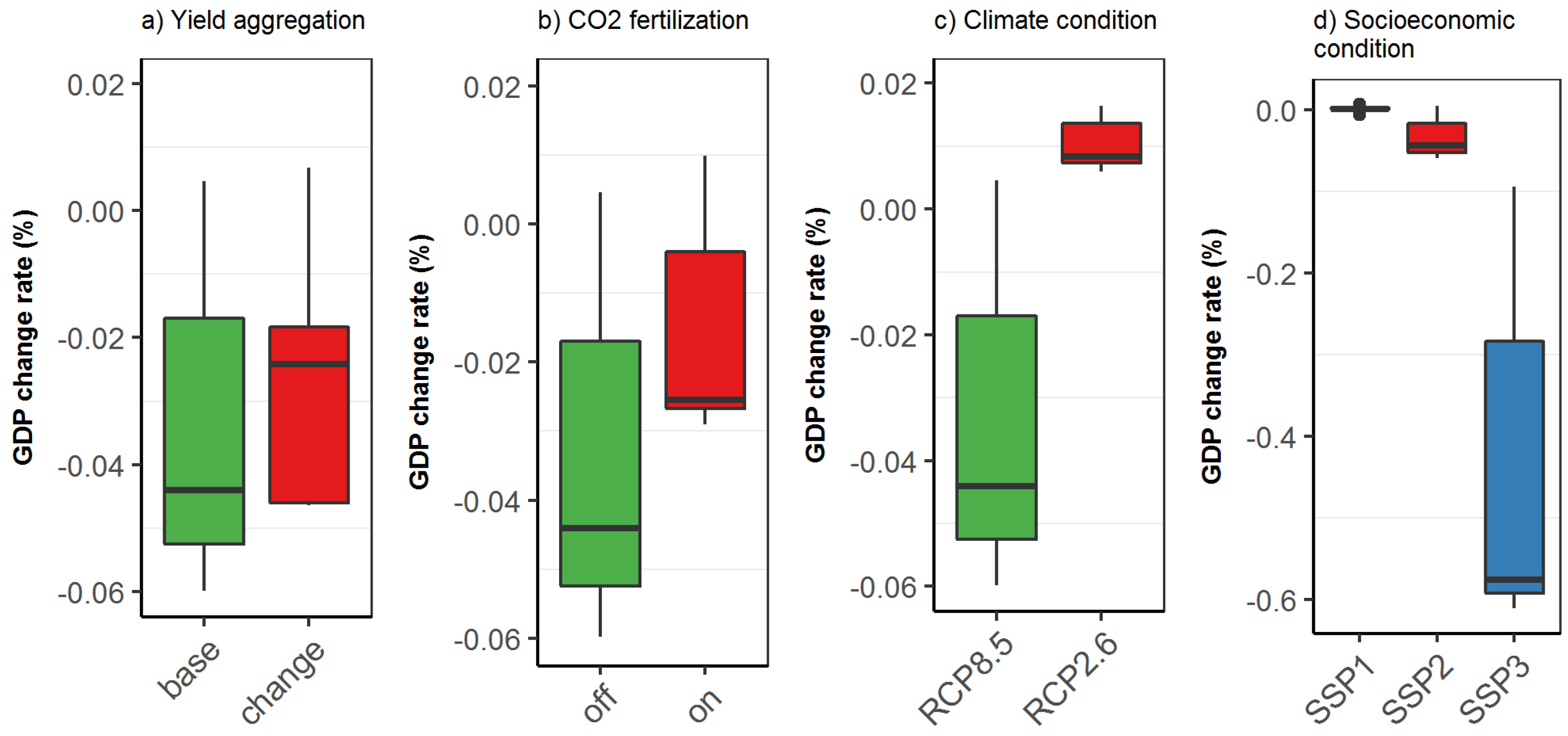
The global total macroeconomic impact (rate of GDP change) in 2100 due to changes in agricultural yield, relative to the corresponding NoCC cases (e.g., scenario 3–scenario 1), is shown in Figure 1. In total, the range of the GDP change was from 0.00% to −0.57%. For the scenario 1 case, which is without gridded land-use change, has no CO2 fertilization, and used SSP2 and RCP8.5, in 2100 the median change is 0.04%. The yield aggregation method produces about half (0.02%) of the change of the no gridded land use case (panel a). However, considering the uncertainty of GCMs, this difference is ambiguous. When focusing on the existence of the CO2 fertilization effect (panel b), the median change is about 0.02%, which is similar to the yield aggregation method effect. The climate change condition is a stronger factor than either the yield aggregation method effect or the CO2 fertilization effect in terms of the macroeconomy. The use of RCP2.6 results in a worldwide rate of GDP loss of −0.01%, which represents an overall positive effect, with all GCMs producing a positive change (panel c). This positive effect would be caused by modest warming. Note that these scenarios do not consider mitigation costs. If mitigation is considered, the mitigation costs would dominate the GDP changes, resulting in clear losses and the climate change impact on yield being much smaller than the mitigation cost (see Figure S3). On the other hand, it can be seen from (panel d) in Figure 1 that the difference depending on the socioeconomic conditions is remarkable in SSP3, with the digits differing by one order of magnitude. The use of SSP3 produces a difference of 0.57%, while the use of SSP1 has little influence.
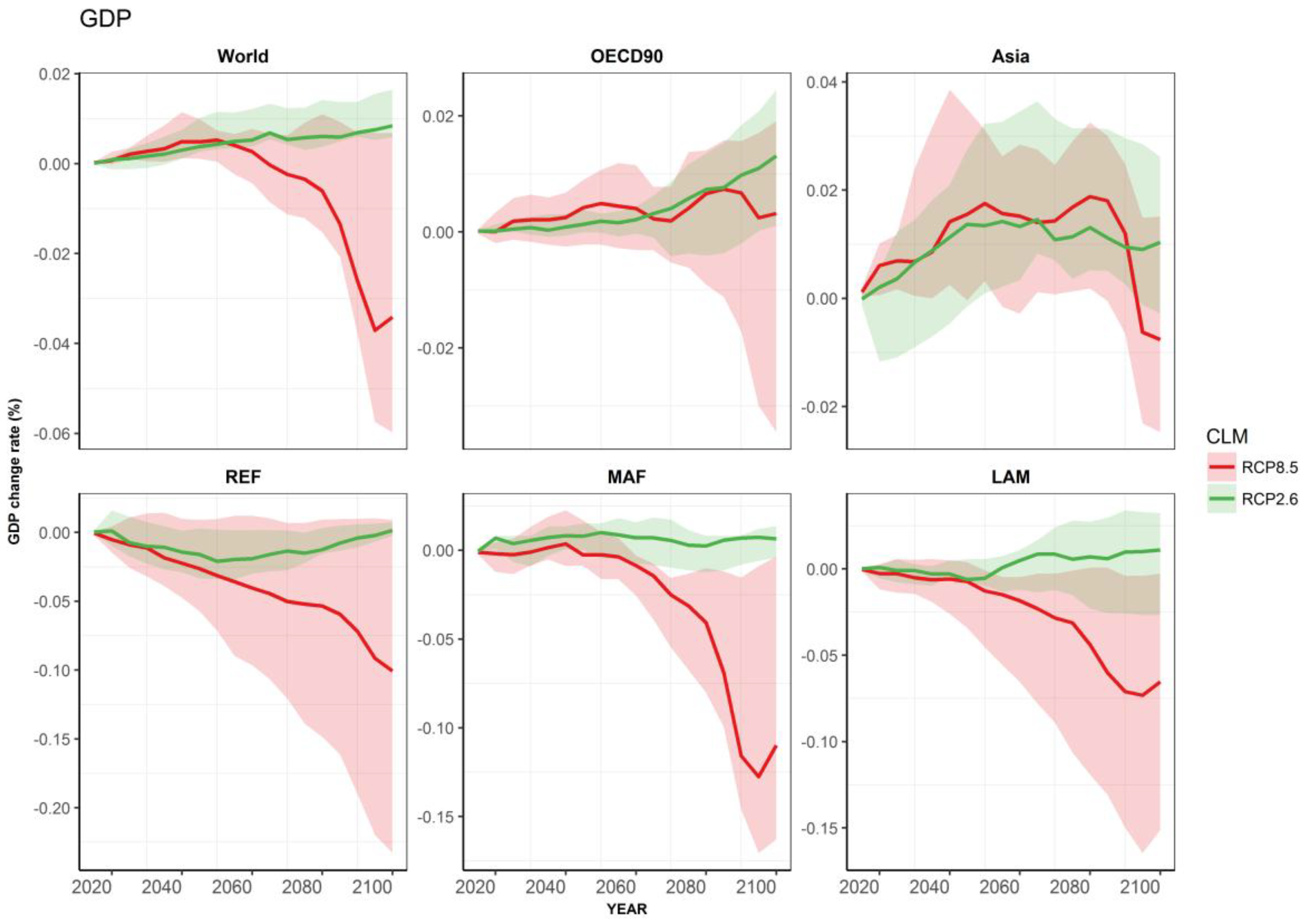
Figure 2 shows time series information about each climate change level, with regional information. From a worldwide perspective, the rate of GDP loss (negative GDP change) increases rapidly after 2050. The range of uncertainty also increases over time. The uncertainty range in RCP8.5 is larger than that in RCP2.6, which is basically driven by crop model outcome (shown later in Figure 4).The increase is not a unique characteristic across the five large regions. For example, the OECD median value is almost stable, while the range of uncertainty increases in the latter half of the century. The median in Asia is also stable and the range of uncertainty is almost constant over time across the scenarios. In contrast, Africa (MAF) and Latin America (LAM) are relatively low-latitude zones that could be sensitive to the effects of global warming. In these countries, RCP8.5 resulted in a higher GDP loss than RCP2.6. Reforming regions (REF; mostly the former Soviet Union) are also likely to have a negative impact in RCP8.5, but the range of uncertainty is large. More detailed regional results indicate that there are some regions or countries that the order of the magnitude is higher than those shown in Figure 2 (e.g., Rest of Asia; XSA in Figure S4). Note that regional heterogeneity is also apparent across the yield aggregation method options and CO2 fertilization assumption differences (Figures S5 and S6).
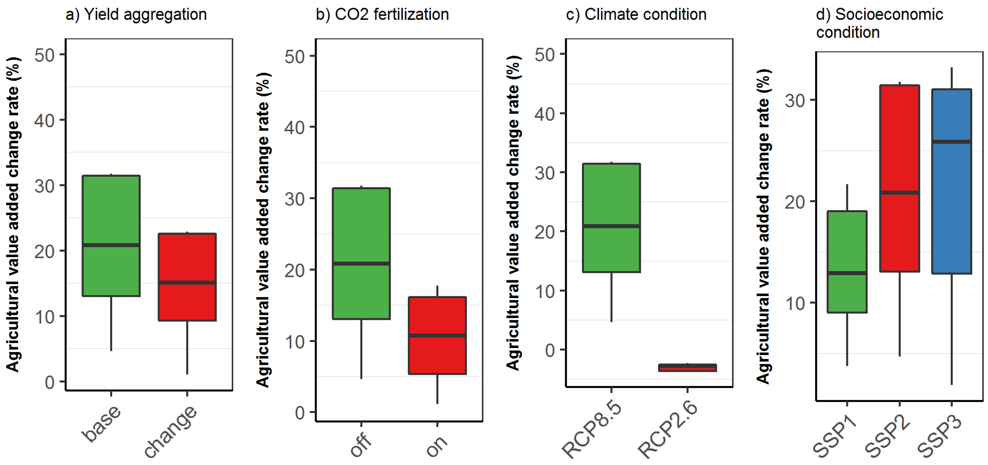
Interestingly, the added agricultural value has much more visible changes than GDP, and the sign is positive, which means an increase in agricultural added value (Figure 3). The food consumption response is much lower than yield change (Figures S7 and S8) due to the price elasticity far less than 1 (Table S6), the basic reactions of the CGE model to the yield changes are expanding the cultivated area (Figure S7). Therefore, the yield negative effect will require additional labor and capital, which will increase the production price and added value of the agriculture sector. On the other hand, these additional labor and capital in agriculture sectors would decrease the resource availability in other industries that would have relatively higher productivity than agriculture sectors, which eventually generates GDP loss as shown above in spite of an increase in added agricultural value. The order of the magnitude is around 10‒30% of changes compared to no climate change cases, which are remarkably large.
3.2. Changes in Agricultural Yield Associated with Climate Change and Its Consequences
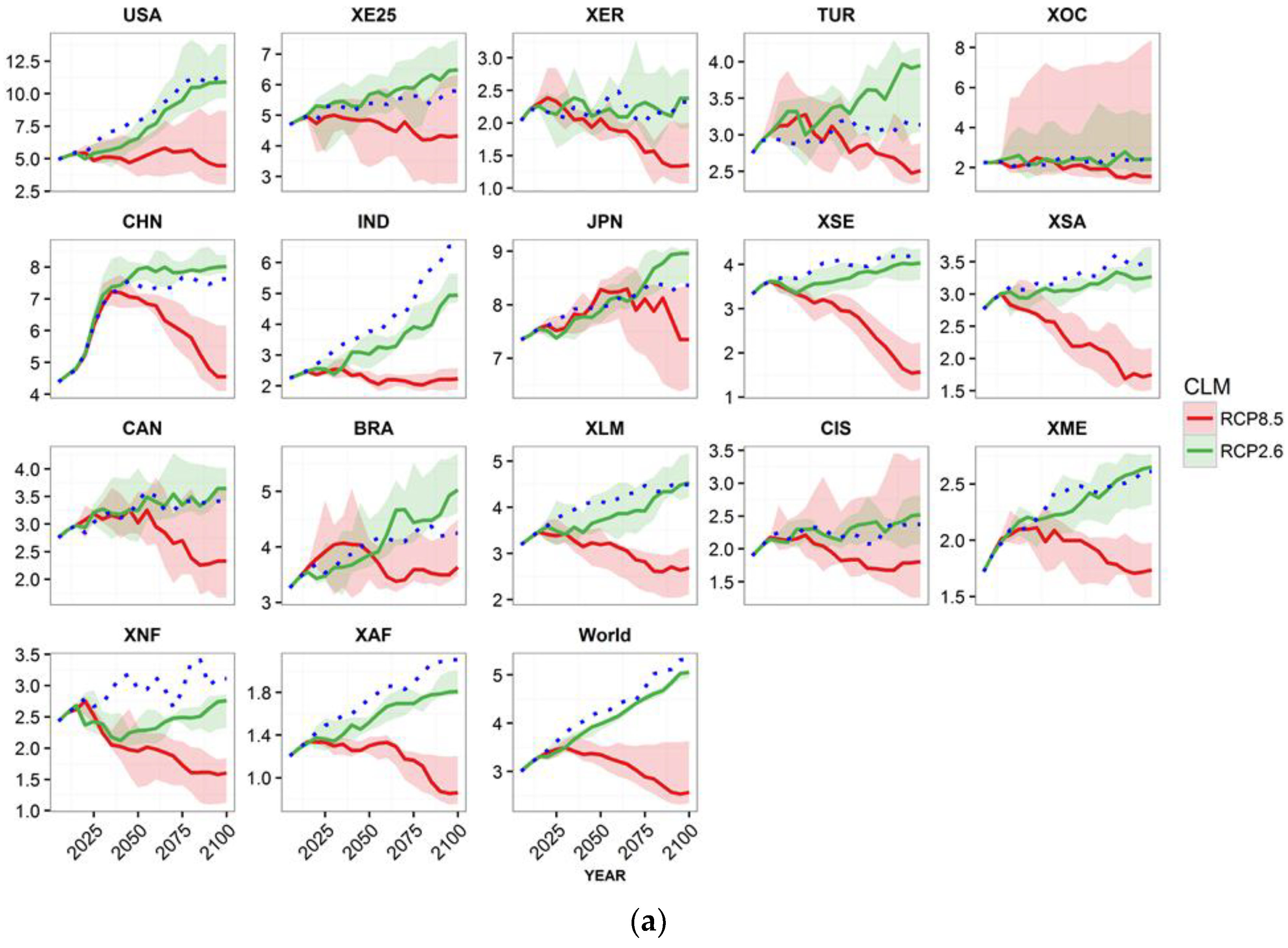
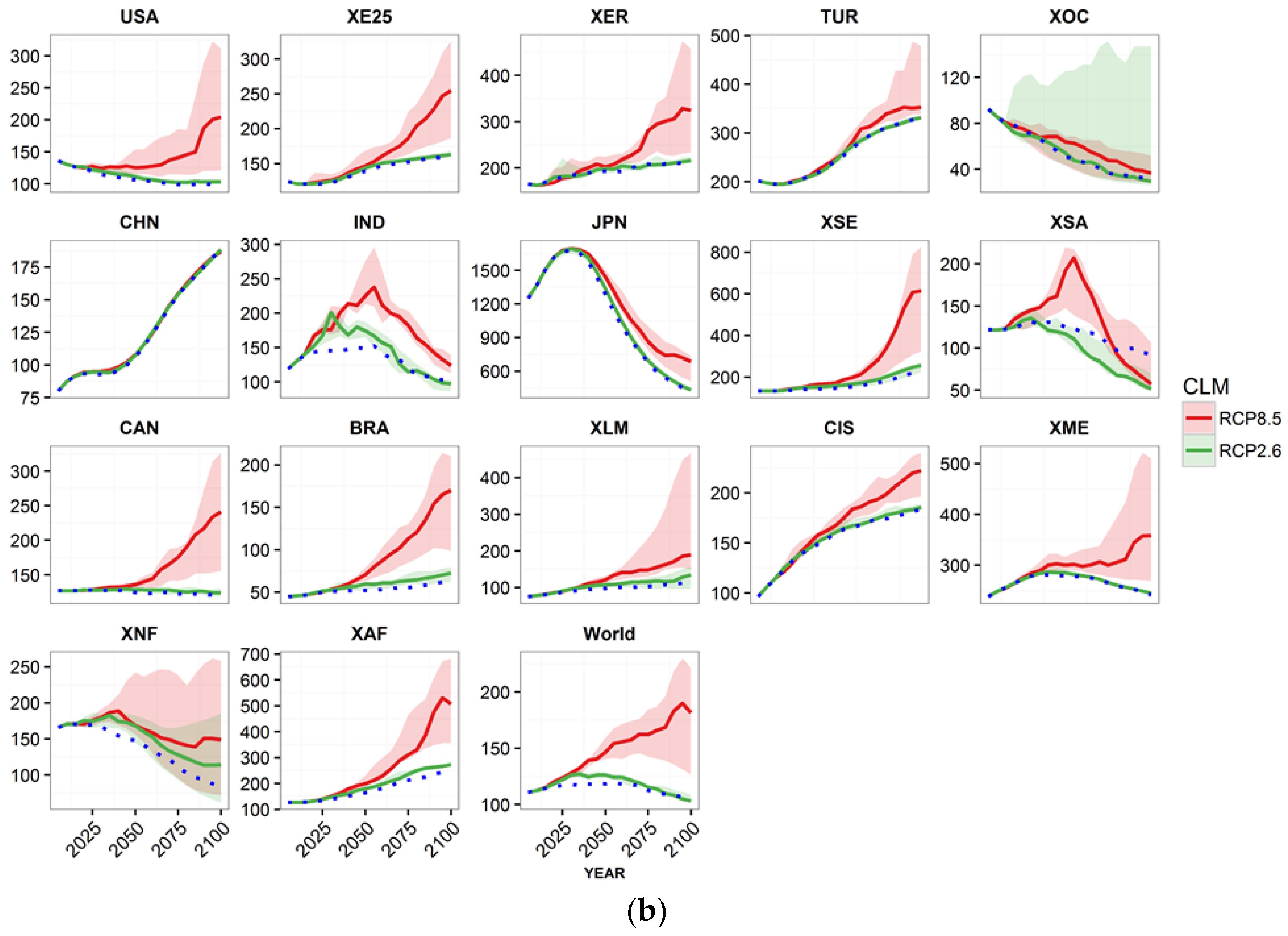
Figure 4 (panel a) shows the average yield of five crops (rice, wheat, other cereals, oil crops, and sugar crops) for AIM/CGE in 17 regions and the global total (see individual crops in Figures S9–S12). The yields are clearly different among the cases with different climate change conditions, i.e., RCP2.6, RCP8.5, and NoCC. The mean global mean yield is currently around 3 t/ha. Because of technological progress, which is mainly caused by the growth of income, the yield increases to about 5 t/ha in the scenario where climate conditions are kept at the current level (NoCC). The RCP2.6 case is similar to the NoCC case. This trend is apparent in the global total, but varies regionally in some cases. For example, the yield in India is about 25% lower for the RCP2.6 case than NoCC, while in China it is slightly larger than NoCC (less than 10%). Although the impact on global average yield is negative in RCP2.6 there is a positive impact on GDP. This is mainly due to the weighting used to calculate the average value. Regional GDP, the impact on yield, and agricultural production has different weighting, and the way that the average is calculated causes discrepancies.
In the RCP8.5 case, there is a substantial decrease in yield. The difference in the global mean decrease from the NoCC decrease is not dissimilar in the first couple of decades of the 21st century, before the influence of climate change becomes apparent but, over time, the deviation becomes large. In 2100, it is almost 3 t/ha, which is almost the same as in 2005. Although there are always uncertainties associated with the use of multiple GCMs, the negative effect on yield is clearly seen. In particular, the remarkable tendency for a deviation from the yield decrease in the NoCC case mentioned above is significant in developing countries such as India (IND), other Asia (XSA), and other Africa (XAF). Even when CO2 fertilization is considered, a similar pattern is apparent, although the negative effect is modest (see Figure S5).
As can be seen from Figure 4 (panel b), the yield decreases lead to a food price increase, which is also discussed in IPCC AR5 and AgMIP literature [3,4,5]. In 2100, the global average price of five major crops in the RCP8.5 case is much higher than in the NoCC and RCP2.6 cases. The RCP2.6 and NoCC cases are similar, and RCP8.5 is around 70% (range of 30 to 120%) higher than NoCC. This price response is higher than that reported in the AgMIP study (0 to 60%). Since the yield information, and the models are different from AgMIP, it is not fully comparable, but one of the reasons could be that AgMIP’s focus is the year 2050, in which the impact of climate change is not projected to be as severe as in 2100.
3.3. Gridded Yield Aggregation Method Effect
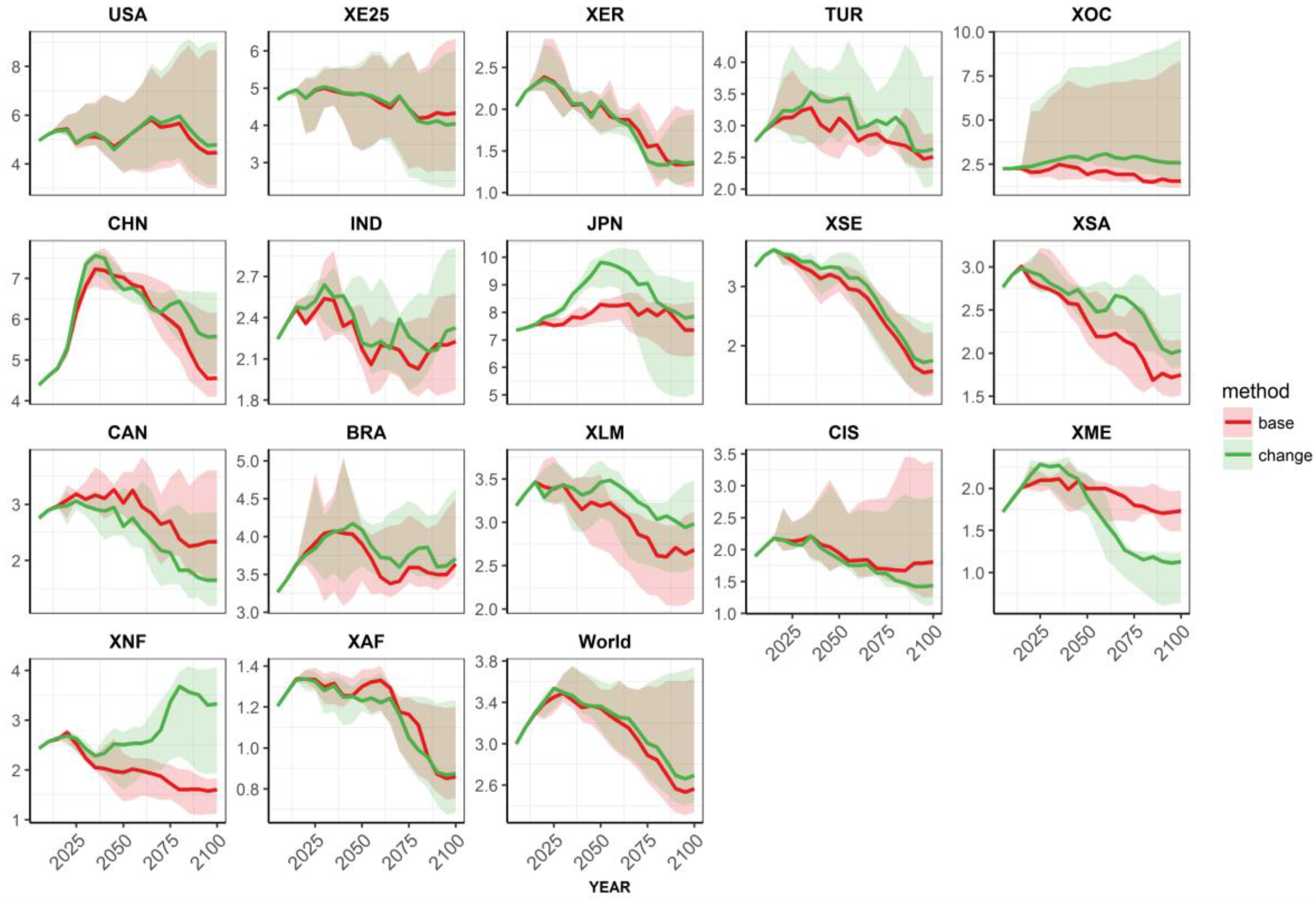
We addressed the changes in GDP associated with aggregation method of gridded yield information in Section 3.1. The next question with respect to this land-use change treatment is how much significant changes are generated in the yield between these two methods. The Figure 5 illustrates yield differences and some regions are quite overlapping, which means land-use change treatment do not change in the macroscale results. However, interestingly, many regions show quite different yield trajectories across the land use treatment. In particular, North Africa (XNF) and the Middle East (XME) are remarkably different regions. Crops specific results are more diverse. These results imply that an analysis that requires regional and crop-specific focuses should deal with the spatial explicit land-use change appropriately.
4. Discussion
The socioeconomic differences cause a relatively large impact on the global macroeconomy in terms of agricultural yield differences. There are two implications from this. First, in the situation where climate mitigation failed, it would be desirable for societal development to be directed toward SSP1 like world in the SSPs context so that the impact of climate change can be kept to a minimum locally and globally. Second, the fact that socioeconomic conditions are a major factor means that further detailed research is required in this area.
One of the focuses of this study is how much the spatially explicit land-use change responded to changes in crop yield due to the influence of climate change on the macroeconomy. Conventional CGE studies have not treated these issues appropriately. From the results of this study, this is found to be a significant factor. It should be noted that the GCM uncertainty could hide the significance of the results of GDP. However, considering the regional variation, the methodology aggregating yield information by using future spatial land-use change is important at the regional or crop specific level. This would imply that methodological improvement may need to be considered for the CGE modeling which might also be better to reconsider the model intercomparison exercise [36].
The macroeconomic impact of changes in agricultural yield associated with future climate change is found to be small compared with the economic analysis of climate effects in other sectors where the large sectors would be 0 point several percentages or even higher [37,38]. For example, in IPCC AR5, [1] reported that a 3.0 °C increase in global mean temperature would lead to around 1 to 3% welfare loss. The most severe climate change case in our study is RCP8.5, which has an increase in global mean temperature of more than 4 °C. The macroeconomic loss in agriculture due to climate change is one order of magnitude less than that of the total impact across all sectors. The magnitude of this loss is similar to that reported in earlier studies [7,9,10]. There are several possible reasons for this. First, the value added by the agricultural sector is small relative to the GDP of the economy as a whole. The current share of agricultural value added is 3.7% of total GDP (Table S5). The GDP in 2100 is projected to increase by about seven times compared to the current value in SSP2, but because most of the growth would originate from secondary and tertiary sectors, the ratio of value added in agriculture in 2100 to GDP is 1.3%. Second, depending on the region, there are some areas where the influence on the macroeconomy is projected to be positive (indicated by negative GDP losses in the figure), which are offset in the global values. However, this offset effect is not significant. Third, the adjustment effect due to international trade could be a factor. However, the value added by the agricultural sector is considered to be the primary reason. Although here we focused on macroeconomic implications in order to obtain climate change impact information that is comparable across sectors, we should note that it does not mean agricultural climate change is less important despite small macroeconomic changes. Rather, they are related to human basic needs and may entail a human health effect [39,40].
With regard to the regional variation, no specific trend could be identified from the regional information, and it is not clear in which region climate change would have a negative influence. It is clear that low latitude regions experienced relatively high impacts, which could be due to a pure climate change effect, but could also be due to the low GDP per capita. In these regions, the value added of agriculture to GDP is higher than developed countries and the economic impact of climate change seems to be higher as well, which suggests that the impacts on GDP could be larger in developing countries.
5. Limitations
There were several limitations of this research. First, we only used one crop model and one economic model, and the results might have been different if multiple models had been used. We believe that additional model inter-comparison experiments are, therefore, necessary. Second, there are some constraints in the use of CYGMA information. (1) The wheat sector yield is biased because CYGMA wheat currently only deals with spring wheat. This aspect of the model should be improved in the future. (2) The yields of crops other than those treated by CYGMA were obtained from LPJml and the two models are not fully consistent. Because the trends in the four major crops were dealt with appropriately, the major outcomes would be unaffected by this treatment. This crop-cover issue should also be resolved in future studies. (3) We experimented limited scenario combinations and there could be much more possibilities such as SSP4 and SSP5, or different climate levels (e.g., RCP45). (4) The study attempts to account for all relevant uncertainties as much as possible considering current model capability, but there are still some missing elements (e.g., the geopolitical international situation and the possibility of transgenic species). As in studies of the impact of climate change in other sectors, particularly for economic analyses, it is difficult to cover all aspects of the subject, although the modeling framework attempts to capture the main factors.
6. Conclusions
This study reveals the macroeconomic impact of climate change in the agriculture sector using an integrated assessment modelling framework. By considering various factors, such as mitigation policy, the yield aggregation method associated with gridded land-use change, GCM uncertainty, and CO2 fertilization, the macroeconomic impact is found to be small (0.02–0.06%), even in the case with the highest level of warming. However, when the socioeconomic condition is changed to SSP3 from SSP2, the scale of the impact increases by an order of magnitude. This study highlights the importance of consideration of future socioeconomic conditions in the agricultural economic implications associated with climate change impacts.
Supplementary Materials
The following are available online at https://www.mdpi.com/2071-1050/10/10/3673/s1, Figure S1: Asia-Pacific Integrated Model (AIM) modeling framework, Figure S2: Ten-year mean annual yield growth rate for the SSP1, SSP2, and SSP3 baseline scenarios, Figure S3: The macroeconomic impact due to mitigation policy (RCP2.6 equivalent) and agricultural yield change for RCP2.6 for five regions and the global total, Figure S4: Macroeconomic impact due to changes in agricultural yield in SSP2 in five regions and as a global total, Figure S5: The macroeconomic impact due to changes in agricultural yield for RCP8.5 with and without CO2 fertilization for five regions and the global total, Figure S6: The macroeconomic impact due to changes in the agricultural yield for RCP8.5 with and without consideration of land-use change for five regions and the global total, Figure S7: Global main indicators’ changes for RCP2.6 (right) and RCP8.5 (left) in 2050 (top) and 2010 (bottom), Figure S8: Food consumption as colorific in take per capita, per day change for the 17 regions of the Asia-Pacific Integrated Model/Computable General Equilibrium (AIM/CGE) and the global average in two climate change cases (green; RCP2.6 and red; RCP8.5) and the no climate change (NoCC) case (blue dot), Figure S9: Yield change of coarse grains for the 17 regions of the Asia-Pacific Integrated Model/Computable General Equilibrium (AIM/CGE) and the global average in two climate change cases (green; RCP2.6 and red; RCP8.5) and the no climate change (NoCC) case (blue dot), Figure S10: Yield change of oil seeds for the 17 regions of the Asia-Pacific Integrated Model/Computable General Equilibrium (AIM/CGE) and the global average in two climate change cases (green; RCP2.6 and red; RCP8.5) and the no climate change (NoCC) case (blue dot), Figure S11: Yield change of rice for the 17 regions of the Asia-Pacific Integrated Model/Computable General Equilibrium (AIM/CGE) and the global average in two climate change cases (green; RCP2.6 and red; RCP8.5) and the no climate change (NoCC) case (blue dot), Figure S12: Yield change of wheat for the 17 regions of the Asia-Pacific Integrated Model/Computable General Equilibrium (AIM/CGE) and the global average in two climate change cases (green; RCP2.6 and red; RCP8.5) and the no climate change (NoCC) case (blue dot), Figure S13: Yield change of five major crops for the 17 regions of the Asia-Pacific Integrated Model/Computable General Equilibrium (AIM/CGE) and the global average in a climate change (RCP8.5) case and the no climate change (NoCC) cases (blue dot), Figure S14: Rice yield for 17 regions in the Asia-Pacific Integrated Model/Computable General Equilibrium (AIM/CGE) and the global average in two gridded yield aggregation method associated with land-use change (red; fixed as base year harvested area and red; changed dynamically) under RCP8.5 and non-CO2 fertilization cases, Figure S15: Wheat yield for 17 regions in the Asia-Pacific Integrated Model/Computable General Equilibrium (AIM/CGE) and the global average in two gridded yield aggregation method associated with land-use change (red; fixed as base year harvested area and red; changed dynamically) under RCP8.5 and non-CO2 fertilization cases, Figure S16: Coarse grain yield for 17 regions in the Asia-Pacific Integrated Model/Computable General Equilibrium (AIM/CGE) and the global average in two gridded yield aggregation method associated with land-use change (red; fixed as base year harvested area and red; changed dynamically) under RCP8.5 and non-CO2 fertilization cases, Table S1. Regional classifications., Table S2: Land use classification, Table S3: Industrial classification, Table S4: List of general circulation models (GCMs), Table S5: Share of primary sector’s value added in total GDP for SSP1, SSP2, and SSP3, Table S6: Price elasticity in 2050 baseline case. The numbers are derived from LES (Linear Expenditure System) consumption function, and Table S7: Income elasticity in 2050 baseline case. The numbers are derived from LES (Linear Expenditure System) consumption function.
Author Contributions
S.F., T.I. and T.H. designed the research; S.F., T.I. and T.K. carried out the simulations; S.F. carried out the analysis of the modeling results; S.F. led the writing of the paper; S.F. created figures; all authors contributed to the discussion and interpretation of the results.
Funding
This research is supported by JSPS KAKENHI Grant Number JP16K18177, JSPS Overseas Research Fellowships, and Environment Research and Technology Development Fund S-14-5 of the Environmental Restoration and Conservation Agency.
Conflicts of Interest
The authors declare no conflicts of interest.
References
- Arent, D.; Tol, R.; Faust, E.; Hella, J.; Kumar, S.; Strzepek, K.M. Key economic sectors and services. In Climate Change 2014: Impacts, Adaptation, and Vulnerability. Part A: Global and Sectoral Aspects; Contribution of Working Group II to the Fifth Assessment Report of the Intergovernmental Panel on Climate Change; Field, C.B., Barros, V.R., Dokken, D.J., Mach, K.J., Mastrandrea, M.D., Bilir, T.E., Chatterjee, M., Ebi, K.L., Estrada, Y.O., Genova, R.C., et al., Eds.; Cambridge University Press: Cambridge, UK, 2014. [Google Scholar]
- Tol, R.S.J. The Economic Impacts of Climate Change. Rev. Environ. Econ. Policy 2018, 12, 4–25. [Google Scholar] [CrossRef]
- Porter, J.R.; Xie, L.; Challinor, A.J.; Cochrane, K.; Howden, S.M.; Iqbal, M.M.; Lobell, D.B.; Travasso, M.I. Chapter 7: Food Security and Food Production Systems; Cambridge University Press: Cambridge, UK, 2014. [Google Scholar]
- Nelson, G.C.; van der Mensbrugghe, D.; Ahammad, H.; Blanc, E.; Calvin, K.; Hasegawa, T.; Havlik, P.; Heyhoe, E.; Kyle, P.; Lotze-Campen, H.; et al. Agriculture and climate change in global scenarios: Why don’t the models agree. Agric. Econ. 2014, 45, 85–101. [Google Scholar] [CrossRef]
- von Lampe, M.; Willenbockel, D.; Ahammad, H.; Blanc, E.; Cai, Y.; Calvin, K.; Fujimori, S.; Hasegawa, T.; Havlik, P.; Heyhoe, E.; et al. Why do global long-term scenarios for agriculture differ? An overview of the AgMIP Global Economic Model Intercomparison. Agric. Econ. 2014, 45, 3–20. [Google Scholar] [CrossRef]
- Reilly, J.; Hohmann, N.; Kane, S. Climate change and agricultural trade. Glob. Environ. Chang. 1994, 4, 24–36. [Google Scholar] [CrossRef]
- Ren, X.; Weitzel, M.; O’Neill, B.C.; Lawrence, P.; Meiyappan, P.; Levis, S.; Balistreri, E.J.; Dalton, M. Avoided economic impacts of climate change on agriculture: Integrating a land surface model (CLM) with a global economic model (iPETS). Clim. Chang. 2016, 146, 517–531. [Google Scholar] [CrossRef]
- Roson, R.; Damania, R. The macroeconomic impact of future water scarcity: An assessment of alternative scenarios. J. Policy Model. 2017, 39, 1141–1162. [Google Scholar] [CrossRef]
- Stevanović, M.; Popp, A.; Lotze-Campen, H.; Dietrich, J.P.; Müller, C.; Bonsch, M.; Schmitz, C.; Bodirsky, B.L.; Humpenöder, F.; Weindl, I. The impact of high-end climate change on agricultural welfare. Science Adv. 2016, 2, e1501452. [Google Scholar] [CrossRef] [PubMed] [Green Version]
- Ciscar, J.C.; Iglesias, A.; Feyen, L.; Szabo, L.; Van Regemorter, D.; Amelung, B.; Nicholls, R.; Watkiss, P.; Christensen, O.B.; Dankers, R.; et al. Physical and economic consequences of climate change in Europe. Proc. Natl. Acad. Sci. USA 2011, 108, 2678–2683. [Google Scholar] [CrossRef] [PubMed] [Green Version]
- van der Mensbrugghe, D. Chapter 14—Modeling the Global Economy–Forward-Looking Scenarios for Agriculture. In Handbook of Computable General Equilibrium Modeling; Dixon, P.B., Jorgenson, D.W., Eds.; Elsevier: Amsterdam, The Netherlands, 2013; Volume 1, pp. 933–994. [Google Scholar]
- Hasegawa, T.; Fujimori, S.; Ito, A.; Takahashi, K.; Masui, T. Global land-use allocation model linked to an integrated assessment model. Sci. Total Environ. 2017, 580, 787–796. [Google Scholar] [CrossRef] [PubMed] [Green Version]
- Fujimori, S.; Masui, T.; Matsuoka, Y. AIM/CGE [Basic] Manual; Version 2012-01; Center for Social and Environmental Systems Research, National Institute Environmental Studies: Tsukuba, Japan, 2012; pp. 1–87. [Google Scholar]
- Bondeau, A.; Smith, P.C.; Zaehle, S.; Schaphoff, S.; Lucht, W.; Cramer, W.; Gerten, D.; Lotze-Campen, H.; MÜLler, C.; Reichstein, M.; et al. Modelling the role of agriculture for the 20th century global terrestrial carbon balance. Glob. Chang. Biol. 2007, 13, 679–706. [Google Scholar] [CrossRef]
- Rosenzweig, C.; Elliott, J.; Deryng, D.; Ruane, A.C.; Müller, C.; Arneth, A.; Boote, K.J.; Folberth, C.; Glotter, M.; Khabarov, N.; et al. Assessing agricultural risks of climate change in the 21st century in a global gridded crop model intercomparison. Proc. Natl. Acad. Sci. USA 2014, 111, 3268–3273. [Google Scholar] [CrossRef] [PubMed] [Green Version]
- Fujimori, S.; Hasegawa, T.; Masui, T.; Takahashi, K.; Herran, D.S.; Dai, H.; Hijioka, Y.; Kainuma, M. SSP3: AIM implementation of Shared Socioeconomic Pathways. Glob. Environ. Chang. 2017, 42, 268–283. [Google Scholar] [CrossRef]
- Fujimori, S.; Dai, H.; Masui, T.; Matsuoka, Y. Global energy model hindcasting. Energy 2016, 114, 293–301. [Google Scholar] [CrossRef]
- Iizumi, T.; Furuya, J.; Shen, Z.; Kim, W.; Okada, M.; Fujimori, S.; Hasegawa, T.; Nishimori, M. Responses of crop yield growth to global temperature and socioeconomic changes. Sci. Rep. 2017, 7, 7800. [Google Scholar] [CrossRef] [PubMed]
- Babel, M.S.; Deb, P.; Soni, P. Performance Evaluation of AquaCrop and DSSAT-CERES for Maize Under Different Irrigation and Manure Application Rates in the Himalayan Region of India. Agric. Res. 2018, 1–11. [Google Scholar] [CrossRef]
- Porwollik, V.; Müller, C.; Elliott, J.; Chryssanthacopoulos, J.; Iizumi, T.; Ray, D.K.; Ruane, A.C.; Arneth, A.; Balkovič, J.; Ciais, P.; et al. Spatial and temporal uncertainty of crop yield aggregations. Eur. J. Agron. 2017, 88, 10–21. [Google Scholar] [CrossRef]
- Ruth, D.; Gernot, K.; Florian, Z.; Wolfram, M. Global economic–biophysical assessment of midterm scenarios for agricultural markets—biofuel policies, dietary patterns, cropland expansion, and productivity growth. Environ. Res. Lett. 2018, 13, 025003. [Google Scholar] [CrossRef] [Green Version]
- Mauser, W.; Klepper, G.; Zabel, F.; Delzeit, R.; Hank, T.; Putzenlechner, B.; Calzadilla, A. Global biomass production potentials exceed expected future demand without the need for cropland expansion. Nat. Commun. 2015, 6, 8946. [Google Scholar] [CrossRef] [PubMed]
- Humpenöder, F.; Popp, A.; Stevanovic, M.; Müller, C.; Bodirsky, B.L.; Bonsch, M.; Dietrich, J.P.; Lotze-Campen, H.; Weindl, I.; Biewald, A.; et al. Land-Use and Carbon Cycle Responses to Moderate Climate Change: Implications for Land-Based Mitigation? Environ. Sci. Technol. 2015, 49, 6731–6739. [Google Scholar] [CrossRef] [PubMed]
- Havlík, P.; Schneider, U.A.; Schmid, E.; Böttcher, H.; Fritz, S.; Skalský, R.; Aoki, K.; Cara, S.D.; Kindermann, G.; Kraxner, F.; et al. Global land-use implications of first and second generation biofuel targets. Energy Policy 2011, 39, 5690–5702. [Google Scholar] [CrossRef]
- Riahi, K.; van Vuuren, D.P.; Kriegler, E.; Edmonds, J.; O’Neill, B.C.; Fujimori, S.; Bauer, N.; Calvin, K.; Dellink, R.; Fricko, O.; et al. The Shared Socioeconomic Pathways and their energy, land use, and greenhouse gas emissions implications: An overview. Glob. Environ. Chang. 2017, 42, 153–168. [Google Scholar] [CrossRef] [Green Version]
- Wise, M.; Calvin, K. GCAM3.0 Agriculture and Land Use: Technical Description of Modeling Approach; Pacific Northwest National Laboratory: Richland, WA, USA, 2011. [Google Scholar]
- Dimaranan, B.V. Global Trade, Assistance, and Production: The GTAP 6 Data Base; Dimaranan, B.V., Ed.; Center for Global Trade Analysis, Purdue University: West Lafayette, IN, USA, 2006. [Google Scholar]
- United Nations, (UN). National Accounts Main Aggregates Database; United Nations: New York, NY, USA, 2013. [Google Scholar]
- Monfreda, C.; Ramankutty, N.; Foley, J.A. Farming the planet: 2. Geographic distribution of crop areas, yields, physiological types, and net primary production in the year 2000. Glob. Biogeochem. Cycles 2008, 22. [Google Scholar] [CrossRef] [Green Version]
- Mueller, N.D.; Gerber, J.S.; Johnston, M.; Ray, D.K.; Ramankutty, N.; Foley, J.A. Closing yield gaps through nutrient and water management. Nature 2012, 490, 254–257. [Google Scholar] [CrossRef] [PubMed]
- Deryng, D.; Sacks, W.J.; Barford, C.C.; Ramankutty, N. Simulating the effects of climate and agricultural management practices on global crop yield. Glob. Biogeochem. Cycles 2011, 25. [Google Scholar] [CrossRef] [Green Version]
- Ito, A.; Inatomi, M. Water-Use Efficiency of the Terrestrial Biosphere: A Model Analysis Focusing on Interactions between the Global Carbon and Water Cycles. J. Hydrometeorol. 2012, 13, 681–694. [Google Scholar] [CrossRef]
- van Vuuren, D.P.; Edmonds, J.; Kainuma, M.; Riahi, K.; Thomson, A.; Hibbard, K.; Hurtt, G.C.; Kram, T.; Krey, V.; Lamarque, J.-F.; et al. The representative concentration pathways: An overview. Clim. Chang. 2011, 109, 5–31. [Google Scholar] [CrossRef]
- Fujimori, S.; Su, X.; Liu, J.-Y.; Hasegawa, T.; Takahashi, K.; Masui, T.; Takimi, M. Implication of Paris Agreement in the context of long-term climate mitigation goals. SpringerPlus 2016, 5, 1–11. [Google Scholar]
- Popp, A.; Calvin, K.; Fujimori, S.; Havlik, P.; Humpenoeder, F.; Stehfest, E.; Bodirsky, B.L.; Dietrich, J.P.; Doelmann, J.C.; Gusti, M.; et al. Land-use futures in the shared socio-economic pathways. Glob. Environ. Chang. Hum. Policy Dimens. 2017, 42, 331–345. [Google Scholar] [CrossRef]
- Hasegawa, T.; Fujimori, S.; Havlík, P.; Valin, H.; Bodirsky, B.L.; Doelman, J.C.; Fellmann, T.; Kyle, P.; Koopman, J.F.L.; Lotze-Campen, H.; et al. Risk of increased food insecurity under stringent global climate change mitigation policy. Nat. Clim. Chang. 2018, 8, 699–703. [Google Scholar] [CrossRef]
- Park, C.; Fujimori, S.; Hasegawa, T.; Takakura, J.Y.; Takahashi, K.; Hijioka, Y. Avoided economic impacts of energy demand changes by 1.5 and 2 °C climate stabilization. Environ. Res. Lett. 2018, 13, 045010. [Google Scholar] [CrossRef] [Green Version]
- Takakura, J.Y.; Fujimori, S.; Takahashi, K.; Hijioka, Y.; Hasegawa, T.; Honda, Y.; Masui, T. Cost of preventing workplace heat-related illness through worker breaks and the benefit of climate-change mitigation. Environ. Res. Lett. 2017, 12, 064010. [Google Scholar] [CrossRef] [Green Version]
- Hasegawa, T.; Fujimori, S.; Takahashi, K.; Yokohata, T.; Masui, T. Economic implications of climate change impacts on human health through undernourishment. Clim. Chang. 2016, 136, 1–14. [Google Scholar] [CrossRef]
- Springmann, M.; Godfray, H.C.J.; Rayner, M.; Scarborough, P. Analysis and valuation of the health and climate change cobenefits of dietary change. Proc. Natl. Acad. Sci. USA 2016, 113, 4146–4151. [Google Scholar] [CrossRef] [PubMed]
Figure 1.
Global total macroeconomic impact due to changes in agricultural yield in the year 2100 considering: (a) yield aggregation method differences (“Base” considers a fixed grid-level harvest map and “Change” considers land-use change at grid level, with both under SSP2), (b) CO2 fertilization (on or off), (c) climate condition, and (d) socioeconomic condition. Boxplots represent the uncertainty of five general circulation models (GCMs). For panels (a,b,c) left, and the center of (d) boxplots are identical because they are the same scenario (RCP8.5), with no CO2 fertilization and no land-use change cases.

Figure 2.
Macroeconomic impact due to changes in agricultural yield in SSP2 in five regions and as a global total (positive means increase compared with baseline). The colors represent climate change level (RCPs). The shaded area is the general circulation model (GCM) range of uncertainty (five GCMs for RCP8.5, and RCP2.6). The lines are the median of five GCMs for each RCP2.6 and RCP8.5. The scenarios in which CO2 fertilization and land-use change are both included are shown. Regional codes are OECD9, OECD regions; Asia, Asia; REF, Reforming region; MAF, Middle East and Africa; and LAM, Latin America. (The mapping procedure from 17 regions is shown in Table S1.)

Figure 3.
Global agricultural value added impact due to changes in agricultural yield in the year 2100 considering (positive means increase compared with baseline): (a) yield aggregation method differences (“Base” considers a fixed grid-level harvest map and “Change” considers land-use change at grid level, with both under SSP2), (b) CO2 fertilization (on or off), (c) climate condition, and (d) socioeconomic condition. Boxplots represent the uncertainty of five general circulation models (GCMs). For panels (a,b,c) left, and the center of (d) boxplots are identical because they are the same scenario (RCP8.5), with no CO2 fertilization and no land-use change cases.

Figure 4.
(a) Mean changes in a) yield and (b) price of five major crops for 17 regions (Table S1) and the global average in two climate change cases (green; RCP2.6 and red; RCP8.5) and the no climate change (NoCC) case (blue dot). The ribbon indicates the range of uncertainty for five general circulation models (GCMs). The units are t/Ha and 1000$/t, respectively.


Figure 5.
Mean yield of five major crops for 17 regions (Table S1) and the global average in two yield aggregation method for land-use change treatment cases (red; fixed as base year harvested area and red; changed dynamically) under RCP8.5 and non-CO2 fertilization cases. The ribbon indicates the range of uncertainty for five general circulation models (GCMs). The units are t/Ha.


Table 1.
List of scenarios.
| Scenario Number | Socioeconomic Condition | Climate Condition | Yield Aggregation Method * | CO2 Fertilization Effect | Mitigation |
|---|---|---|---|---|---|
| 1 | SSP2 | NoCC | Base | ||
| 2 | SSP2 | NoCC | Change | ||
| 3 | SSP2 | RCP8.5 | Change | ||
| 4 | SSP2 | RCP8.5 | Change | X | |
| 5 | SSP2 | RCP8.5 | Base | X | |
| 6 | SSP1 | NoCC | Base | ||
| 7 | SSP1 | RCP8.5 | Base | ||
| 8 | SSP3 | NoCC | Base | ||
| 9 | SSP3 | RCP8.5 | Base | ||
| 10 | SSP2 | RCP2.6 | Base | ||
| 11 | SSP2 | RCP2.6 | Base | X |
* If the yield aggregation is based on the current harvest gridded map, it shows Base. If the gridded land use change is taken, it is “Change.”
© 2018 by the authors. Licensee MDPI, Basel, Switzerland. This article is an open access article distributed under the terms and conditions of the Creative Commons Attribution (CC BY) license (http://creativecommons.org/licenses/by/4.0/).
Share and Cite
MDPI and ACS Style
Fujimori, S.; Iizumi, T.; Hasegawa, T.; Takakura, J.; Takahashi, K.; Hijioka, Y. Macroeconomic Impacts of Climate Change Driven by Changes in Crop Yields. Sustainability 2018, 10, 3673. https://doi.org/10.3390/su10103673
AMA Style
Fujimori S, Iizumi T, Hasegawa T, Takakura J, Takahashi K, Hijioka Y. Macroeconomic Impacts of Climate Change Driven by Changes in Crop Yields. Sustainability. 2018; 10(10):3673. https://doi.org/10.3390/su10103673
Chicago/Turabian StyleFujimori, Shinichiro, Toshichika Iizumi, Tomoko Hasegawa, Jun’ya Takakura, Kiyoshi Takahashi, and Yasuaki Hijioka. 2018. "Macroeconomic Impacts of Climate Change Driven by Changes in Crop Yields" Sustainability 10, no. 10: 3673. https://doi.org/10.3390/su10103673
Note that from the first issue of 2016, this journal uses article numbers instead of page numbers. See further details here.