Agricultural Water Productivity-Based Hydro-Economic Modeling for Optimal Crop Pattern and Water Resources Planning in the Zarrine River Basin, Iran, in the Wake of Climate Change

Abstract

For water-stressed regions/countries, like Iran, improving the management of agricultural water-use in the wake of climate change and increasingly unsustainable demands is of utmost importance. One step further is then the maximization of the agricultural economic benefits, by properly adjusting the irrigated crop area pattern to optimally use the limited amount of water available. To that avail, a sequential hydro-economic model has been developed and applied to the agriculturally intensively used Zarrine River Basin (ZRB), Iran. In the first step, the surface and groundwater resources, especially, the inflow to the Boukan Dam, as well as the potential crop yields are simulated using the Soil Water Assessment Tool (SWAT) hydrological model, driven by GCM/QM-downscaled climate predictions for three future 21th-century periods under three climate RCPs. While in all nine combinations consistently higher temperatures are predicted, the precipitation pattern are much more versatile, leading to corresponding changes in the future water yields. Using the basin-wide water management tool MODSIM, the SWAT-simulated water available is then optimally distributed across the different irrigation plots in the ZRB, while adhering to various environmental/demand priority constraints. MODSIM is subsequently coupled with CSPSO to optimize (maximize) the agro-economic water productivity (AEWP) of the various crops and, subsequently, the net economic benefit (NEB), using crop areas as decision variables, while respecting various crop cultivation constraints. Adhering to political food security recommendations for the country, three variants of cereal cultivation area constraints are investigated. The results indicate considerably-augmented AEWPs, resulting in a future increase of the annual NEB of ~16% to 37.4 Million USD for the 65%-cereal acreage variant, while, at the same time, the irrigation water required is reduced by ~38%. This NEB-rise is achieved by augmenting the total future crop area in the ZRB by about 47%—indicating some deficit irrigation—wherefore most of this extension will be cultivated by the high AEWP-yielding crops wheat and barley, at the expense of a tremendous reduction of alfalfa acreage. Though presently making up only small base acreages, depending on the future period/RCP, tomato- and, less so, potato- and sugar beet-cultivation areas will also be increased significantly.

1. Introduction

Food and water security will pose a great challenge in the near future due to rapid growth of population and often unsustainable water usage. The renewable water resources per capita in the Middle East and North Africa (MENA), as the most water- scarce regions of the world, are expected to decline from 750 to 500 m³ by 2025, while the water withdrawals will increase by up to 50% [1].

Natural and anthropogenically induced climate change will act as an additional external driver threatening the future food security by exacerbating the water shortage, and, concomitantly, the decrease of crop production, as temperatures and irrigation water requirements increase [2]. All of this holds particularly for the Middle East, including Iran, where groundwater reserves diminish at an alarming rate [3].

Improving the management of agricultural water use is of utmost importance, as irrigation water uses account for 70% of the global freshwater withdrawals, particularly due to the fact that the irrigated areas have dramatically increased in the 20th century, providing now about 40% of the world’s food [4,5]. In addition, agriculture has also an important role in the economy, in terms of the Global Gross Domestic Product (GDP), especially in developing countries, although its share has been decreasing over the last twenty years [6]. Thus for Iran the GDP contribution of agriculture decreased from 23 to 9% [7], although the irrigated lands increased by 17% between 2003 and 2008 [8], confirming the low economic productivity of agriculture. Moreover, about 90% of the food demands are derived from agriculture supplies in Iran, but with a cost of exploitation of 92% of the available freshwater resources [5], which indicates that the economic agricultural return on water use is outstandingly low in Iran.

The agricultural production will also need to be increased globally by 70% up to year 2050, due to a 40%-projected population increase [9]. The situation is even worse for developing countries where the food production should be doubled by that time [10]. FAO predicts that only 10% of the global production growth (21% in developing countries) can be achieved by agricultural land expansions with the remainder coming from crop yield enhancements [11].

For a long-term sustainable water resources management for agriculture it is important to quantify and evaluate the possible impacts of climate change scenarios on the future water availability and crop production potentials. Previous publications evaluated the impacts of climate change on the water resources using hydrologic simulation models that are based on GCM-predictions [12,13]. These and numerous other studies indicate that climate change will have undeniable impacts on the hydrology, namely, streamflow changes in a basin, which ultimately affects the water availability there.

For example, the impacts of climate change on the crop yield, food security, and crop water demands in sub-Saharan Africa and the North China Plain are investigated by Chijioke et al. [14] and Mo et al. [2], respectively, using different crop prediction and simulation models. These studies show that climate change may have either beneficial or harmful effects on the crop extent and productivity in irrigated or rain-fed agricultural lands. Other recent studies focus on the analyses of the impacts of a changing climate and agricultural demands on the water management and crop production [15,16] and indicate that climate change will lead to hydrologic changes and thus alter crop yields and crop water productivity (CWP), so that some adaptation strategies are required.

Over recent years, many publications on optimizing crop pattern and water allocation to maximize crop productions and economic benefits and to enhance the agricultural water management have appeared. A multi-crop planning (MCP) optimization model that is based on a nonlinear programming (NLP) algorithm was utilized for cropping pattern and water allocation by Bou-Fakhreddine et al. [17] to maximize the net financial return. Firstly, two linear formulations and a relaxed version were established from the NLP and then the MCP problem is solved by implementing two meta-heuristic algorithms, Simulated Annealing (SA) and Particle Swarm Optimization (PSO). Fazlali and Shourian [18] optimized water allocation by considering optimum cropping pattern for the Arayez plain in Iran, using the Shuffled Frog Leaping Algorithm coupled with MODSIM [19] and employing irrigations depths and cultivation areas as decision variables. However, the authors did not consider the CWP index, impacts of climate change, and management of the conjunctive water uses. In fact, few of these issues have been addressed by Fereidoon and Koch [20] who employed a MODSIM-LINGO-PSO algorithm to maximize the economic benefits of Karkheh Dam in Iran, in terms of water allocation for agriculture, under the impact of future climate change. The authors separated the optimization into a three-stage procedure, wherefore first the MODSIM allocates the available water of Karkheh Dam, with its inflow being simulated by the SWAT-hydrological model. Then, a linear optimization to maximize the crop yields in response to different assumed levels of available water is carried out, and, finally, a PSO algorithm is used to maximize the economic return.

The purpose of the current research is to jointly optimize the crop pattern and irrigation planning under climate change- and cropping pattern scenarios and so to maximize the net economic agricultural benefits and increase the crop production, altogether considering the constraints of limited available water resources. This objective is achieved by using an integrated hydro-economic model that consists of a combination of the CSPSO (Constrained Stretched Particle Swarm Optimization) method and MODSIM water management and planning model as a simulation-optimization approach.

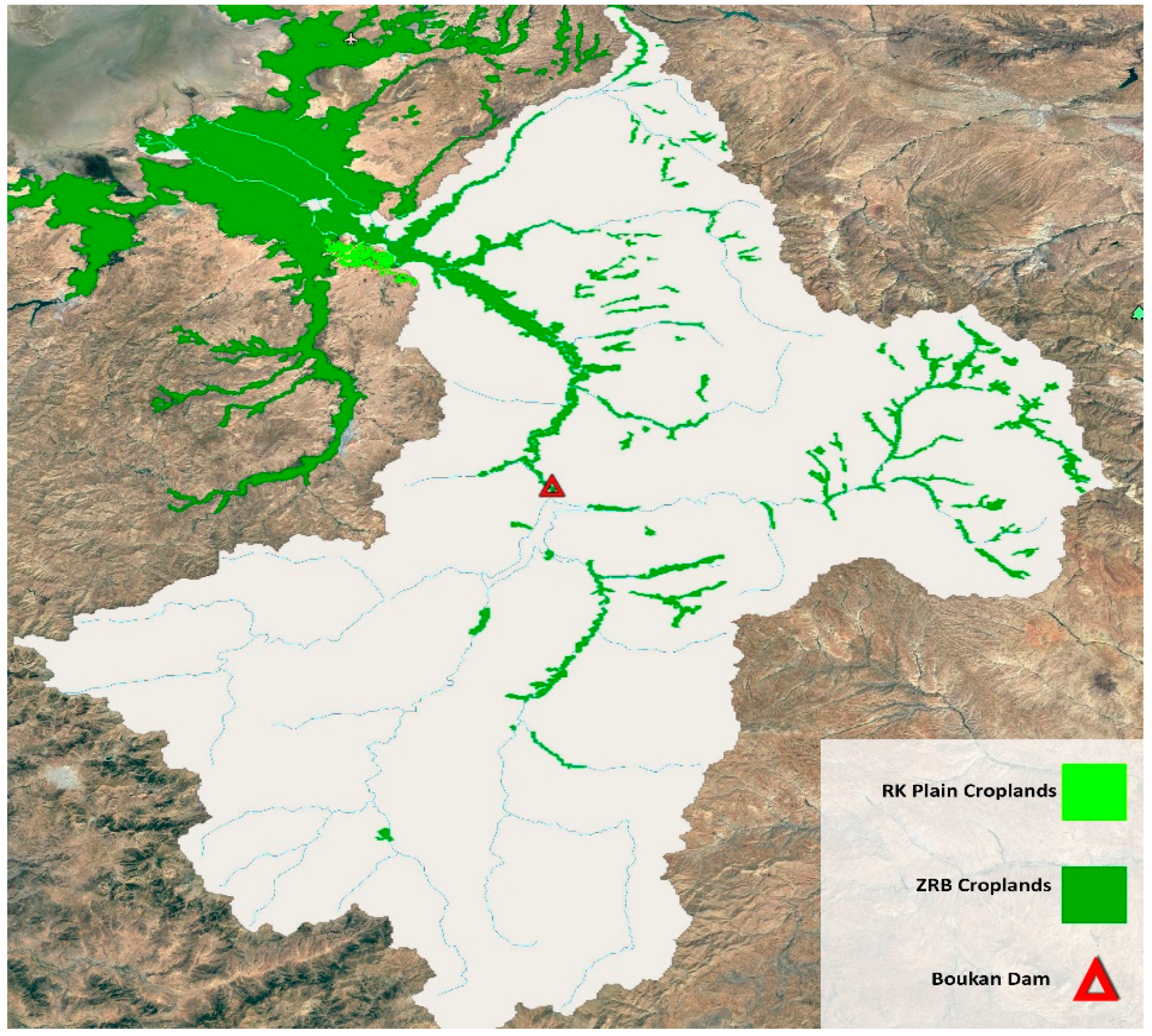
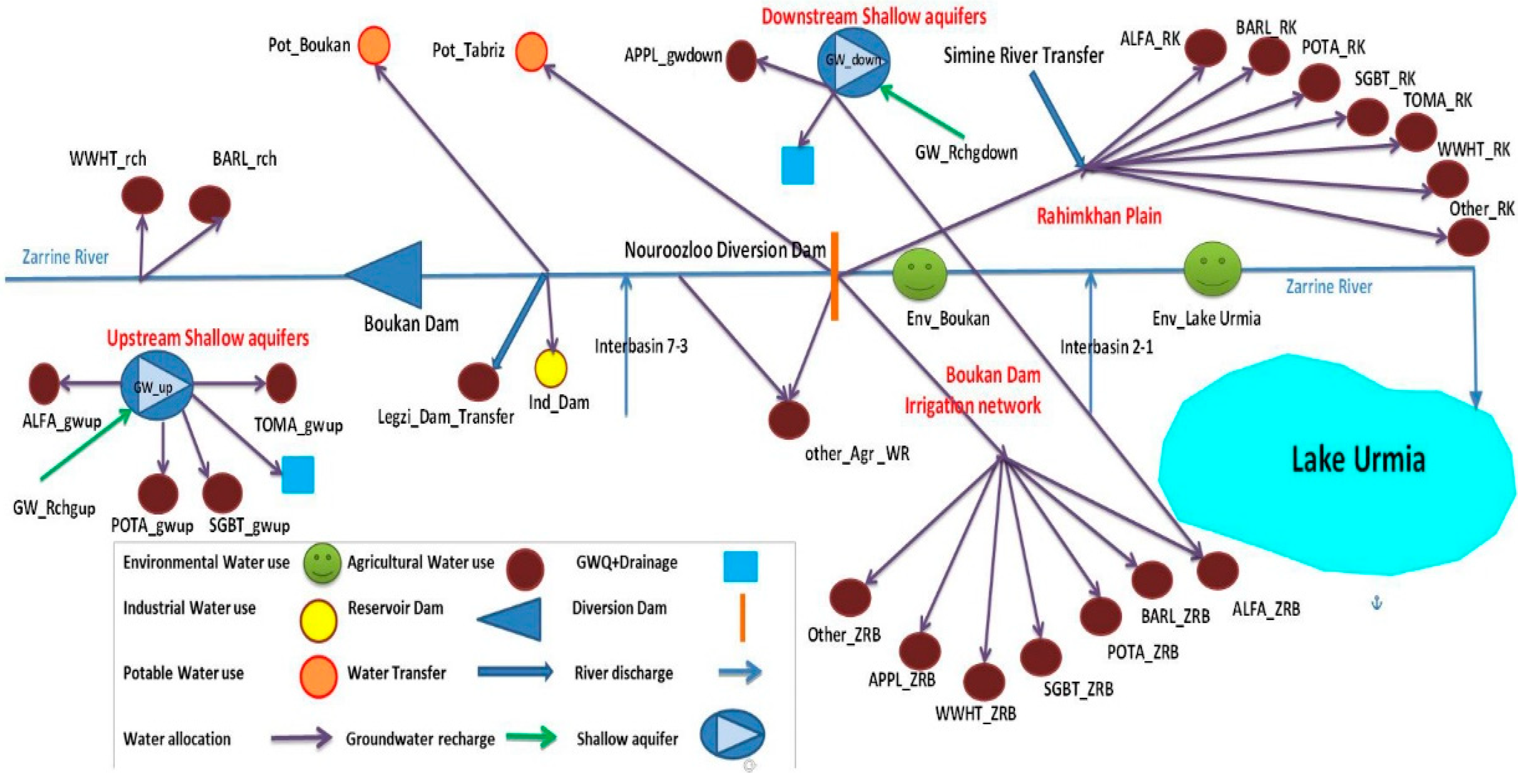
The research area is the Zarrine River Basin (ZRB) belonging to the basin of Lake Urmia (LU), which has been shrinking tremendously over the recent decades. The impacts of climate change scenarios on the water resources and the crop production will be evaluated while considering the crop pattern scenarios for the irrigated croplands using the available water supply sources, namely, the Boukan Dam as the most important water management infrastructure of the region, as well as inter-basin discharges from river reaches and groundwater shallow aquifers.

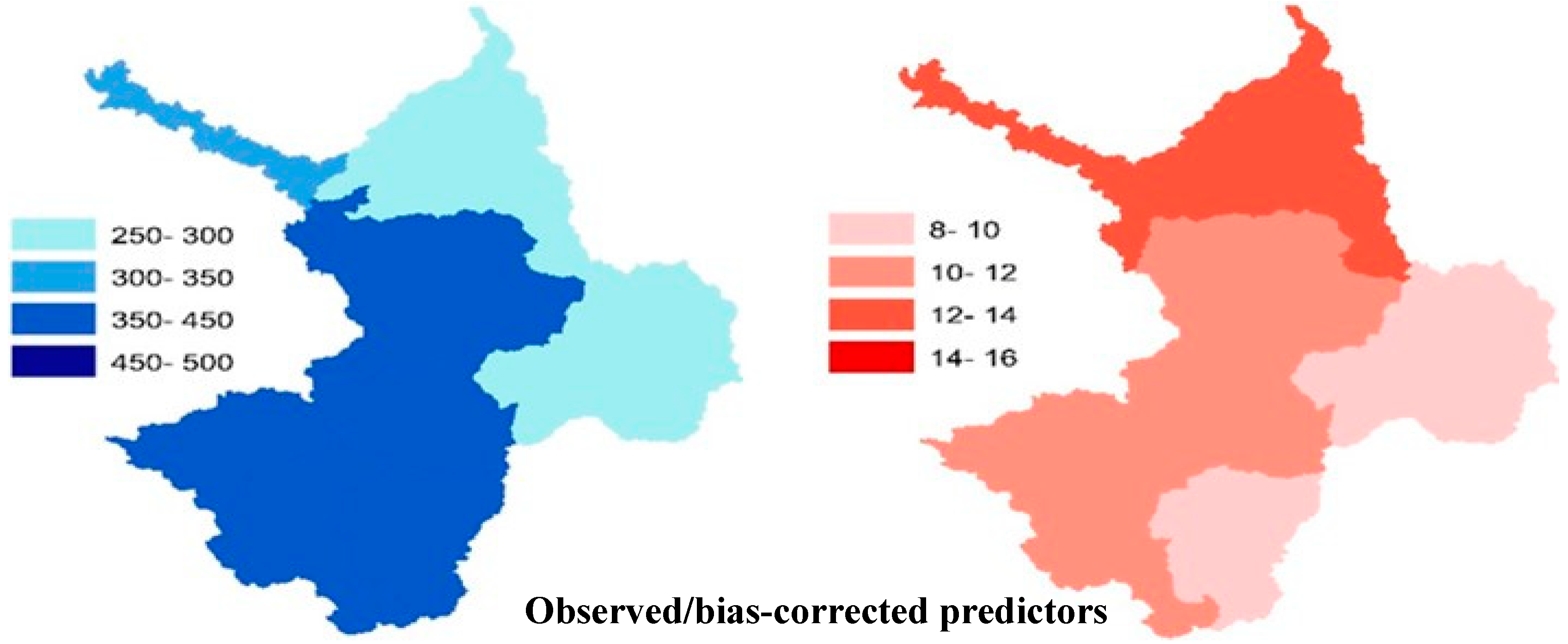
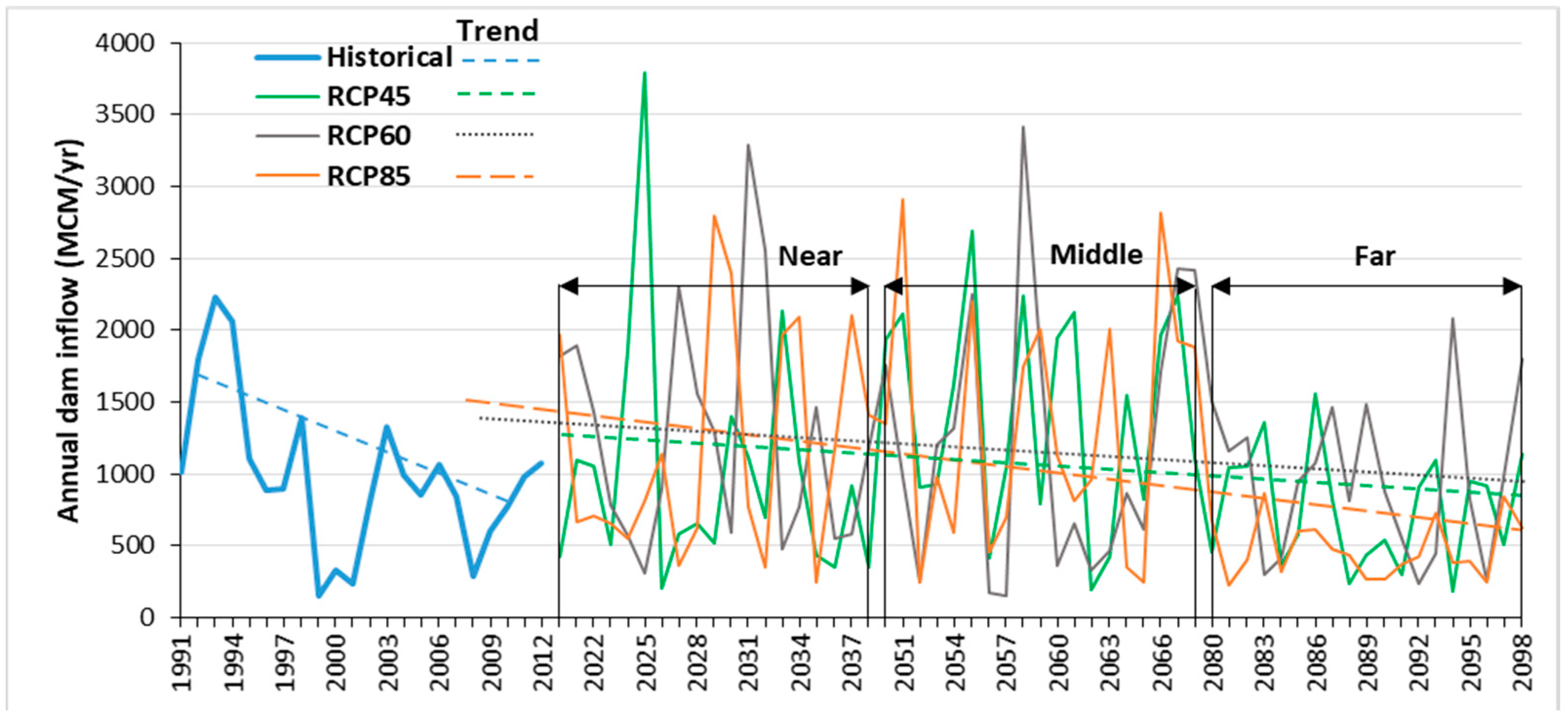
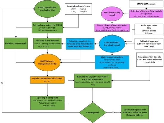
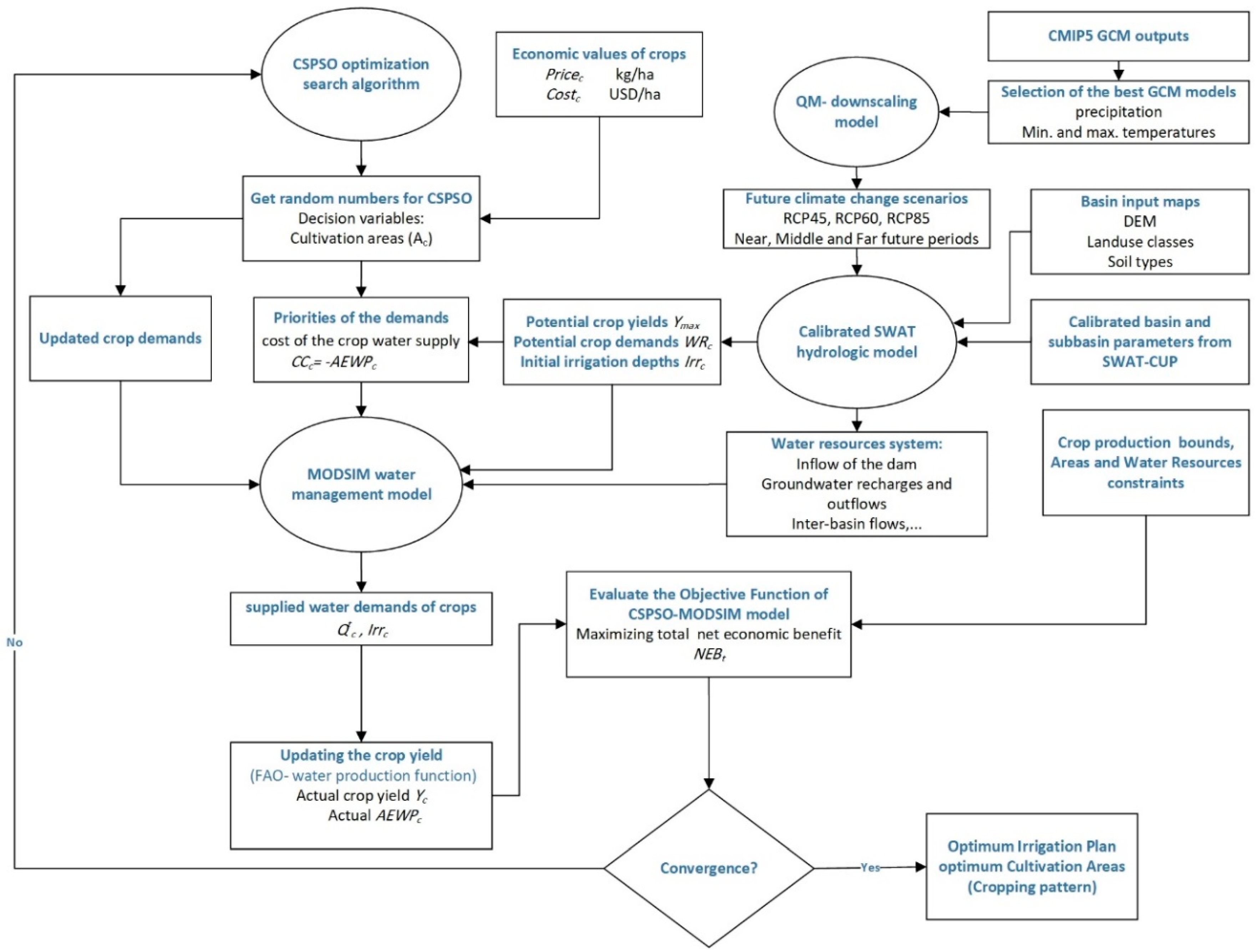
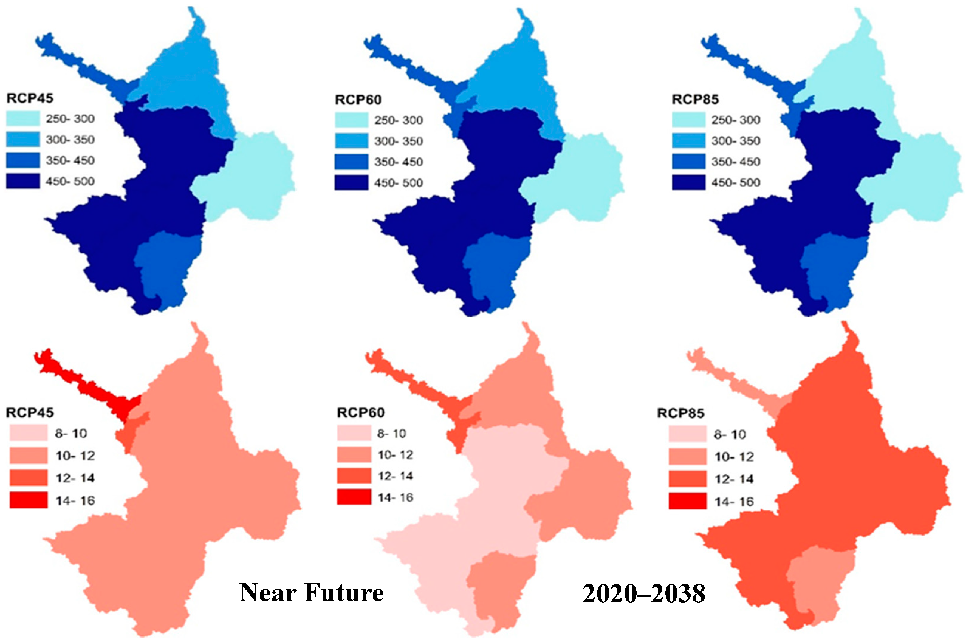
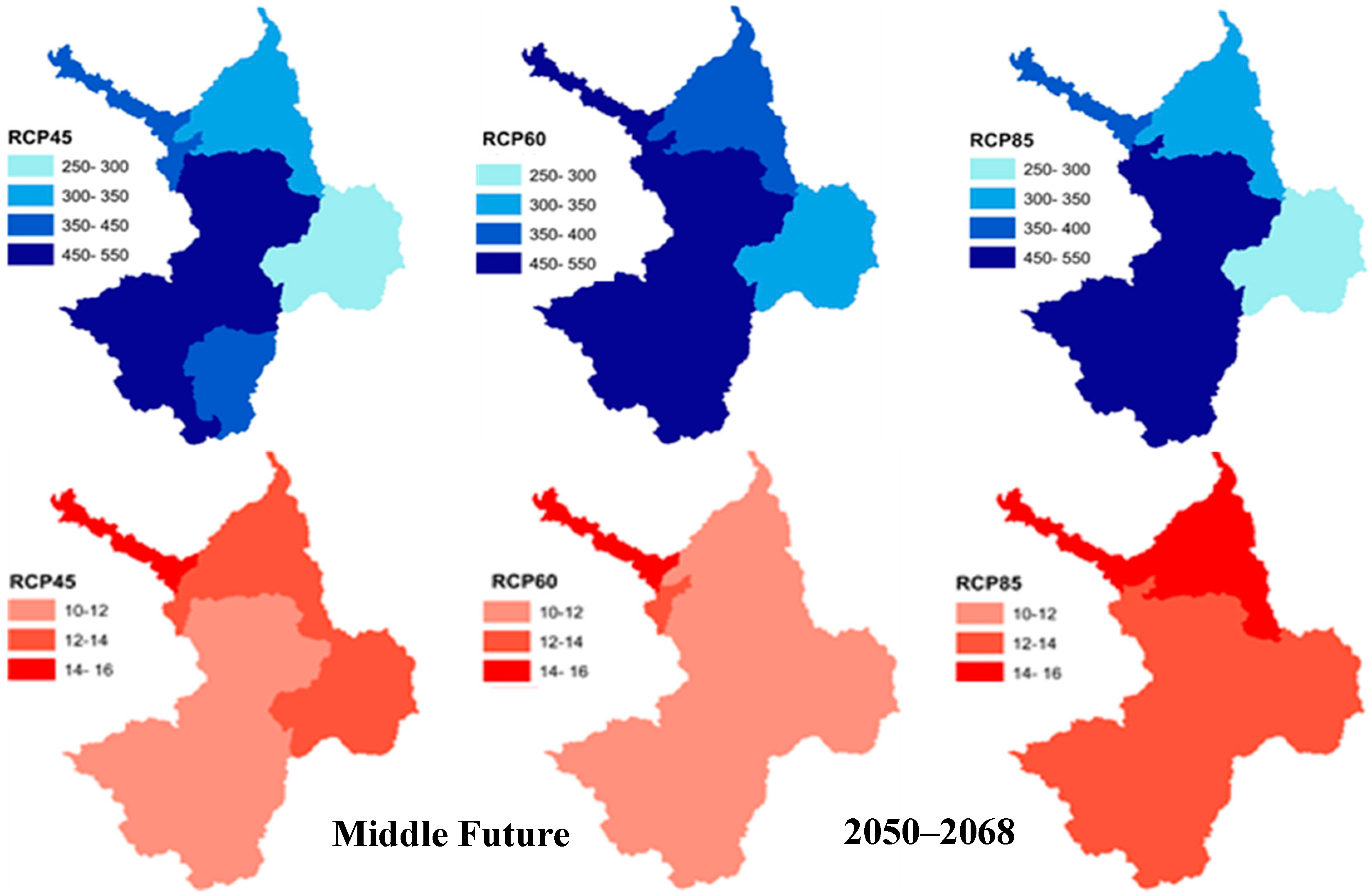
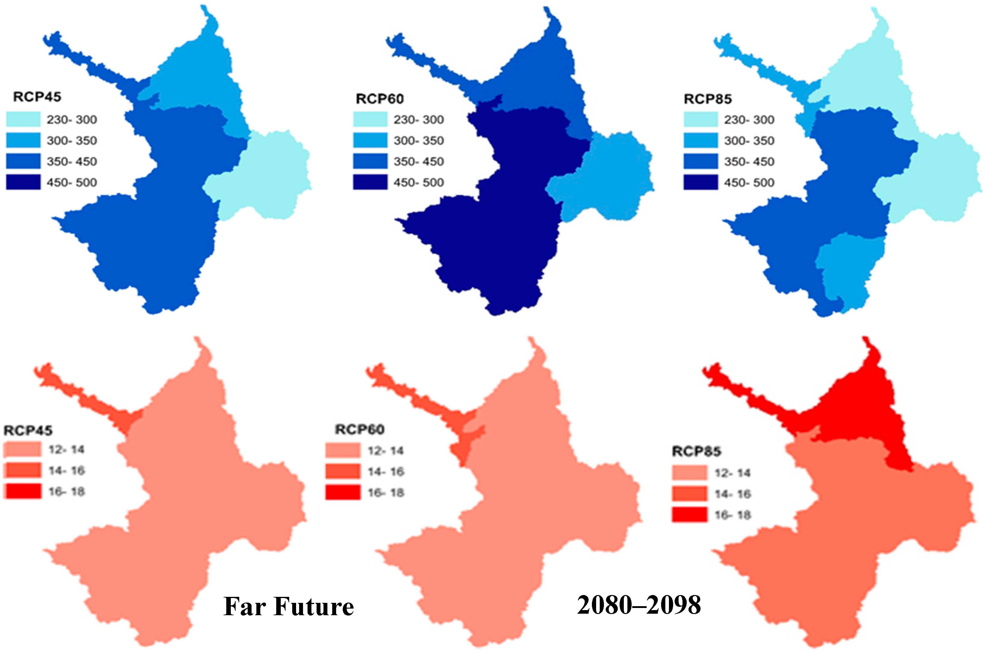
To simulate the basin’s water resources, i.e., the inflow of the Boukan Reservoir, interbasin flows, groundwater recharges, and other hydrologic variables of the ZRB in response to the changing climate, future (up to year 2098) downscaled climate predictors (min. and max. temperatures, precipitation) are taken from the recent study of Emami and Koch [13], and entered into the river basin hydrologic model, SWAT, which is firstly calibrated and validated for the discharge and then for the crop yields by adjusting the crop parameters and crop water requirements. Next, a water planning and management simulation model is prepared, using MODSIM for managing the conjunctive agricultural water uses (Q) in the river basin, by respecting the water-distribution priority constraints imposed for the basin as a whole. The model is then adjusted to allocate the available water to the major crop arable areas of the ZRB based on the crop water productivity (CWP) and the net economic benefit (NEB) of the crop production, both of which are combined in an index of agro-economic water productivity (AEWP). Finally, to enhance the crop production and the economic efficiency of the MODSIM-recommended water management policy, a Constrained Stretched Particle Swarm Optimization (CSPSO) algorithm is developed and fully coupled with the MODSIM in order to maximize the total NEB of the ZRB as the objective function and, consequently, the crop production, based on the AEWP- and Q-combination. The optimal arable crop areas and corresponding irrigation schedules are determined while using this CSPSO-MODSIM model under the constraints of arable areas for the irrigation plots and three different cereal crop pattern scenarios when considering three impact scenarios of climate change (RCP45, 60, and 85) for three future periods (near, middle, and far).

2. Study Region and Data

2.1. The Zarrine River Basin

The Zarrine River is the main inflow source of the LU, the largest inland wetland of Iran which used to be the largest lake in the Middle East before it dwindled significantly in recent decades, with detrimental effects on the surrounding ecosystems of the lake. The Zarrine River Basin (ZRB) is located in northwestern Iran, south of LU between 45°46′ E to 47°23′ W longitude and 35°41′ S to 37°44′ N latitude (see Figure 1). The total length of the main channel is about 300 km and most of its course stretches through a mountainous area. The basin covers an area of about 12,000 km², including parts of Kurdestan and the West and East Azarbaijan provinces, wherefore its larger portion is mountainous with an elevation of up to 3297 m and the smaller one is rather plain with an elevation going down to 1264 m. The big cities of the basin are namely Miandoab, Shahindej, Tekab, and Saghez.

The climate of the region varies from semi-wet cold or wet-cold in the mountain areas to semi-dry in the vicinity of LU. The average annual temperature varies between 8 and 12 °C while the annual precipitation (rain and snow) in the basin varies between 200 mm/year in the lower catchment area and 800 mm/year in the mountains. The maximum snowfall is recorded mostly in the south and west of the basin with snow heights varying from 5 to 63 mm/year.

The Boukan Dam/Reservoir is the largest operating dam of the ZRB, with a gross storage capacity of 760 Million m³ (MCM) and a live storage capacity of 654 MCM. 51% of its water is used for agricultural irrigation and the remainder for the supply of drinking and industrial water and environmental rights (826 MCM/year totally).

The agricultural areas within the basin cover a total area of 74,318 ha, all irrigated by both groundwater and surface water resources, including water from the Boukan Reservoir, as the crop-growing season there is mostly during the dry months between spring and autumn.

The current applied irrigation efficiency is about 38% for the areas that are irrigated by the surface water from the dam and the river, and 50% for the areas using groundwater resources; all numbers that are lower than the averages of most developing countries (45%) and developed countries (60%) [21], indicating a non-efficient use of surface water due to outdated irrigation methods and systems with a large loss of water through evaporation and seepage. However, advanced irrigation technologies that enhance the irrigation efficiency, can have negative effect on river flow, as a higher efficiency rarely decreases water consumption, which are usually associated with a reduction in recoverable return flows and an increase in crop yields and crop transpiration [22,23].

It should also be noted that the area of irrigated land has been increased by 36% from 1976 to 2013 [24], and this in spite of a catastrophic 88% decrease of the LU surface and ensuing environmental and ecological crises.

The irrigated croplands of the ZR Basin are demonstrated in Figure 2, including the current irrigated croplands of the ZRB (green) and the future agricultural development plan of ZRB, namely Rahimkhan (RK) Plain (light green) located in the downstream of the Boukan Dam.

The main agricultural crops of the ZRB as well as the RK include alfalfa (ALFA), apple (APPL), barley (BARL), potatoes (POTA), sugar beet (SGBT), tomatoes (TOMA), and wheat (WWHT), and these are the ones that are considered in this study.

2.2. Data

The data needed for this study in the ZRB is gathered from different available sources. Most of the data is required for the set-up of the SWAT-hydrologic model, namely, various geospatial maps and hydro-climate time series.

The Digital Elevation Map (DEM) with a spatial resolution of 85 m was produced by the Iranian surveying organization. The land-use classification map of the basin, demonstrating the situation in year 2007, was obtained from the Agricultural Statistics and the Information Center of the Ministry of Agriculture [25] and it has a resolution of 1000 m and distinguishes 10 land use classes. The soil map of the watershed was extracted from the Food and Agriculture Organization (FAO) digital soil global map, with a spatial resolution of 10 km of and eight types of soils within two layers.

The daily climate input data includes maximum and minimum temperatures and precipitation over the period of 1987 to 2015 and was obtained from the Iranian Meteorological Organization (IRIMO) for six synoptic stations that were located in or close to the ZRB (see Figure 1). Missing data in the records were filled in using the inverse distance weighting (IDW) interpolation method. As the daily data for other climate variables, including solar radiation, wind, and relative humidity, were unavailable, they were generated using the weather generator (WGEN) module of SWAT model based on monthly averages of the synoptic stations of Iran.

Daily streamflow data for six gauging stations of the Zarrine River (Figure 1) were obtained from the Iran Ministry of Energy for the period 1987 to 2012.

The crop and irrigation data, namely, crop irrigation sources, planting, irrigation and harvesting dates, or water demands were taken from Ahmadzadeh et al. and MOE [22,26]. The observed crop yields are gathered from MOA [25] and the additional economic crop data were gathered from SCI and MOA [27,28].

3. Methodology: Development of an Integrated Hydro-Economic Model for Optimal Water Management and Crop Pattern

3.1. Basic Concepts of an Optimal Hydro-Economic Model

Generally, the greater the water-use productivity and economic efficiency, the lower are the conflicts over scarce water resources and the additional financial and environmental burdens in an agriculturally exploited basin, like the ZRB. Enters the fundamental concept of hydro-economics, which stipulates that water demands can be represented as value-sensitive water demand functions, so that water-uses at different locations and times have varying economic benefits [29]. The next step is then to set up a hydro-economic model, which is a solution-oriented model for investigating the water management tradeoffs and improving the economic efficiency of water allocation by incorporating the economic value of agricultural water in the heart of the water management model. This model represents a spatially distributed water resources system, infrastructure, management options, and economic values comprehensively [29]. In the third and final step, such a hydro-economic model may be applied to simulate agricultural crop pattern strategies, with the goal to find that optimal multi-crop pattern that somehow maximizes the economic crop profits, while adhering to the various constraints of the limited water resources, hydrology, and various environmental regulations. Mathematically, this amounts to the set-up of a classical constrained (nonlinear) optimization problem, wherefore (1) the forward problem, i.e., the objective or cost function, is computed by the hydro-economic model, simulating the hydrological constraints by classical hydrological models, and (2) the minimization of that objective function is done by some kind of an optimization routine (e.g., [20]).

In this section, an innovative hydro-economic model for the ZRB is developed using such a simulation-based optimization approach to coordinate multiple factors, including water allocation, crop production pattern, and economic gains. More specifically, the optimization problem is defined as a constrained optimization (CO) problem which searches for the optimal allocation of irrigated crop pattern under the constraints of the limited water resources and other demands that should be satisfied. Eventually, the objective of the optimization search algorithm is to maximize the agro-economic productivity, i.e., the economic net benefit of a crop per unit water use, given that the latter is limited in the study region and it may be even more so in the future under the impacts of imminent climate change there [13].

The decision variables of the optimization are the cultivated areas of major crops for a particular, politically given combination of required crop distribution and agricultural demand regions. The constraints of the optimization algorithm in this study are defined based on the allowable range of arable areas and cereal crop pattern limits (for more details see Section 3.8).

3.2. Modules of the CSPSO-MODSIM Integrated Hydro-Economic Model

The individual modules (hydrological, water management, agro-economic) of the hydro-economic model are developed in this research while using different simulation models (GCM, QM, SWAT, MODSIM) that were bound together with an optimization method (CSPSO). The flow chart of the connection of the models and processes in the integrated hydro-economic model is presented in Figure 3, from which the main steps are retrieved as follows:

-

Predicting climate change weather scenarios using CMIP5-GCMs predictors that are subsequently downscaling by QM.

-

Simulating the future hydrologic changes and crop yields with the calibrated SWAT river basin hydrological model using the QM climate projections as input drivers.

-

Setting up the basin-wide water management and planning module, MODSIM, to allocate the future agricultural water uses that are based on environmental/demand priority constraints.

-

Optimizing the crop arable areas and the related irrigation schedule using the agricultural water productivity- based hydro-economic model, CSPSO-MODSIM.

Details of each of the above modeling steps are described in the following sub-sections.

3.3. Predicting Future Climatic Scenarios by Updated Quantile Mapping

Regarding the projections of future climate change scenarios, they are mostly taken from Emami and Koch [13] who used several climate models (GCMs) of the CMIP5 archive [30], as mentioned in the fifth IPCC report [31] to select the most suitable one based on a climate model’s skill to simulate the past climate in terms of minimum and maximum temperatures and precipitation. For assessing the impacts of climate change on the regional scale, the climate predictors of the selected GCM models were then downscaled using a recently-coming-to-the-fore statistical downscaling method, namely, QM (Quantile Mapping) [32,33], which proved to have better prediction performances than the more commonly used classical statistical downscaling model (SDSM). We forego a detailed description of the QM-downscaling method and refer the reader to [13].

In the first step of the QM method, the monthly biases of the future GCM-simulated climate variables between year 2020 to 2098 are removed while using a trend-preserving bias correction, namely, the ISI-MIP approach [32]. In this approach, the GCM-simulated temperatures (min. and max.) are corrected applying an additive correction factor CT_j and for the precipitation and a multiplicative correction factor CP_j to each month of a year (j = 1, …, 12) of the GCM-simulated precipitation. In the second step a new, updated quantile mapping method [33] is used to correct the daily biases of the temperatures and precipitation in each month (e.g., all Januaries) using EDCDFm and CNCDFm CDF-(cumulative distribution function) matching methods, respectively. Emami and Koch [13] proved that these QM-variants perform better than other statistical downscaling methods in removing biases in the GCM-climate predictors for the study region by delivering much better correlations with the observed predictands (temperatures and precipitation) at the high-resolution, local scale, and of all this without almost no extra computational costs.

3.4. SWAT-Simulation of the Hydrological Processes in the Agricultural Watershed

3.4.1. Model Setup and Calibration

The Soil Water Assessment Tool (SWAT) model is a physically-based, river basin-scale, time continuous simulation model that operates on a daily time step. Although this model has originally been developed to mainly simulate the impacts of land management practices in large and complex watersheds [34], it is widely used as a long-term rainfall-runoff model and efficient hydrologic simulator of water quantity and quality, so that it has increasingly being used to investigate climate change impacts on agro-hydrological systems [12,35].

The SWAT model requires quite a wide range of input data, as described in Section 2.2. To represent the large-scale spatial heterogeneity of the study basin more precisely, the SWAT modeled domain, i.e., the major basin, is divided into several sub-basins, which are usually delineated with the help of the topographic DEM using the ARCSWAT extension of ARCMap program. Then, each sub-basin is parameterized using a set of HRUs (Hydrologic Response Units), which are based on a unique combination of soil and land cover and management. For the SWAT-model of the ZRB, 11 sub-basins with a total of 908 HRUs have been defined.

After the parameterization of the SWAT-model’s input data entries is done by using the stochastic sequential uncertainty fitting version 2 (SUFI-2) optimization algorithm, embedded in the SWAT-CUP decision-making framework [36]. Various kinds of objective functions as measures for the goodness of the fit of the modeled to the observed streamflow are available in the SUFI-2 algorithm, wherefore Krause et al. [37] indicates that for a reliable calibration and validation of the model, a combination of different efficiency criteria, such as the coefficient of determination R², the Nash–Sutcliff efficiency coefficient NSE, and bR² (b is the slope of the regression line between observed and simulated streamflow), should be considered.

In the present application, the calibrated input parameters of the model have been taken from Emami and Koch [13], where further details of the calibration/validation as well as of the model setup are presented. Basically, the optimal range of model input parameters was determined hierarchically sub-basin-wise, from the utmost upstream sub-basin (11) outlet down to the main outlet of the basin.

Based on the SUFI-sensitivity analysis, 24 model parameters were shown to be sensitive parameters for affecting the stream discharge, out of which the SCS curve number (CN2), the groundwater delay time (GW_DELAY), and the moist bulk density of the soil (SOL_BD) turned out to be the three most sensitive variables. With these optimized parameters, good fits of the modeled to the observed discharges were obtained at the six streamflow stations (sub-basin outlets) for the calibration (1998–2012) and the validation (1991–1997) periods, with average R² > 0.7, NSE > 0.6 and bR² > 0.5, which, according to the classification that was proposed by Moriasi et al. [38], is considered to be satisfactory. As the SUFI-computed uncertainty of the calibrated model that is quantified by the P- and the R-factor (see [13,39]) has average values of R > 0.75 and P close to 1, there is enough confidence in the calibrated SWAT-model for the ZRB.

3.4.2. Predicting the Impacts of Future Climate Change on the Hydrologic Cycle

It is important to evaluate the hydrologic responses to future changes of climate for improving adaptive water management, as the variability of precipitation and temperature in terms of trends and extremes will eventually increase the likelihood of severe and irreversible negative impacts on the ecosystem, including lakes and rivers. To that avail, the future downscaled climatic scenarios i.e., the QM-bias corrected predictions of the minimum and maximum temperatures and precipitation are employed as weather input drivers of the calibrated basin-wide hydrologic simulation model, SWAT. As a result, the future hydrologic cycle and the available water resources of the ZRB under the climate change can be assessed, especially the input of the dam, the Inter-basin discharge of the river reaches, the groundwater recharges and the withdrawals of the shallow aquifers.

3.4.3. Crop Yield Simulation and Calibration of the Potential Crop Yield

The SWAT model is also capable of simulating crop productions and yields efficiently, as has been shown in many publications (e.g., [40,41]). To do this in the ZRB, the current management operations of the various crops there are specified initially in the SWAT model, together with the corresponding planting and harvesting dates and the irrigation sources, based on information that was given by Ahmadzadeh et al. [22]. The crop yields for seven major crops in the ZRB are then calibrated by adjusting a set of effective parameters in the model, until the averages of the simulated crop yields of the basin match those of the observed ones (gathered from MOA [25]) in a reasonable manner. These simulated crop yields are then extracted from the SWAT file output.hru to represent the potential crop yields of the ZRB. The reservoir characteristics, irrigation losses and essential demands are considered through the water use management (.wus) and reservoir (.res) SWAT- data files.

3.5. Agro-Economic Water Productivity and Net Economic Benefit

For a better management of the future water resources in a water-scarce region, such as the ZRB, it is necessary to make the water supply- and/or the irrigation system as efficient as possible in economic and water resources perspectives. Because of the competition of the different stakeholders for the scarce freshwater resources in the region, not only for agriculture, a paradigmatic policy shift is required from (a) maximizing productivity per unit of area to (b) maximizing productivity or economic value per unit of consumed water [42], as both the irrigated agriculture’s land base and the water supplies are continuously being depleted and reallocated, in order to produce even more agricultural crops. To achieve this policy shift, the net benefits of the water used, should be enhanced by prioritizing more economic efficient crops i.e., higher productivity per unit of water, while the water use should be constrained to the allocated water resources for agricultural water-use.

The crop-water productivity CWP_c (kg/m³) is defined as the ratio of amount of crop yield that is produced Y_c (kg/ha) to the amount of water applied per unit crop area Q_c (m³/ha) during the crop’s production [43]. The next step is then to define the agro-economic water productivity AEWP_c (USD/m³) as the ratio of net total economic value of crop NEB_c (USD) to the total amount of water Q^t_c (m³) supplied under the priority constraints that were provided by MODSIM (see following subsection) [44]:

AEWP_c = NEB_c/Q^t_c = [(Price_c × Y_c − Cost_c) × A_c]/Q^t_c = (Price_c × Y_c − Cost_c)/Irr_c

(1)

where Price_c (USD/kg) is the selling price of the crop, Cost_c (USD/ha) is the total production costs of the crop, A_c (ha) is the crop cultivation area, Irr_c = Q^t_c/A_c (m) is the irrigation water height, and the other variables are as defined above.

Based on the definitions above, optimizing the water resources allocation can be an important measure for increasing agro-economic water productivity AEWP_c in areas where the water is scarce like ZRB. In this study, a water management model for deficit irrigation is developed to determine the allowable agricultural water, which at the first stage the potable, industrial, and environmental water demands (essential demands) are supplied according to their higher priorities as a constraint and then the remaining available water will be allocated to the agricultural water-uses, i.e., different crop demands based on their AEWPs. Finally, for boosting the net economic benefits NEB_c as the ultimate objective of this study, the combination of agro-economic water productivity AEWP_c and total allocated water Q^t_c is maximized through an optimization algorithm. As in Equation (1), the Price_c and Cost_c are constant for each crop, the total crop economic benefit will also be increased.

3.6. MODSIM Water Resources Management and Planning Module

The MODSIM simulation model is a generalized river basin network model for developing basin-wide strategies of short-term water management, long-term operational planning, drought contingency planning, water rights analysis, and conflict resolution between different water users [19,45]. This model has enjoyed widespread application across the world to simulate operations, as mentioned [20,46,47,48].

The core idea behind MODSIM is to represent a complex river basin system by a flow network consisting of coupled sequences of nodes and links, with the former symbolizing storage components, such as reservoirs and aquifers, points of inflow, demands, diversions, and river confluences, and the latter representing river reaches, pipelines, canals, and stream-aquifer interconnections defining stream depletions from pumping and return flows from seepage and other water applications. Further network elements of the model consist of unregulated inflows, reservoir operating targets, consumptive and instream flow demands, evaporation and channel losses, reservoir storage rights and exchanges, and stream-aquifer modeling components. In addition, various surface and ground water resources with their inter-relationships can be represented by highly nonlinear, non-convex, or discontinuous equations [49]. Details on how each of the components is modeled and calculated in the model can be found in Fredericks et al. [19].

The model sequentially solves a linear optimization problem within the confines of mass balance throughout the network over the planning period by means of a highly efficient network flow optimization (NFO) algorithm solved with the Lagrangian relaxation algorithm RELAX-IV [50]. More specifically, the following constrained flow optimization problem is solved for each time interval (t = 1, …, T) over the planning horizon:

$$Minimize{\displaystyle \sum }_{k\in A}{c}_k{q}_k$$

(2)

Subject to

$${\displaystyle \sum }_{k\in O_i}{q}_{k-}{\displaystyle \sum }_{k\in O_i}{q}_{k=b_{it};\mathrm{for}\mathrm{all}\mathrm{nodes}i\in N}$$

(3)

$$l_k\le q_k\le u_k;\mathrm{for}\mathrm{all}\mathrm{links}k\in A$$

(4)

where A is the set of all links in the network; N is the set of all nodes; q_k is the integer valued flow rate in link k; c_k are cost weighting factors, i.e., the water right priorities per unit flow rate in link k; b_it is the (positive) gain or (negative) loss at node i at time t; I_i the set of all links terminating at node i (inflow links); O_i the set of all links originating at node i (outflow links); and, l_k and u_k are lower and upper bounds, respectively.

The cost factor c_k for accounting for active storage and demand links priorities are generally calculated while using the following formula:

c_k = −(50,000 − 10 × PR_k)

(5)

where PR_k is the integer priority ranking that ranges between 1 and 5000 for the reservoirs or the demands, where the negative sign states that high-rank nodes (1, 2, etc.) are given more weights in the minimization of the cost function (Equation (2)).The cost factor may also include economic factors that are defined in this study for the crop demand links as the cost of the crop water supply (cc_c) based on the agro-economic water productivity index AEWP_c (Equation (1)), i.e., cc_c = −AEWP_c, which means that more water should be allocated to a crop that provides more economic benefits than others for the same amount of water supplied.

The schematic network of the MODSIM ZRB model with the various demand nodes are represented in Figure 4. These demand nodes can be categorized into four groups: (1) the network of the dam croplands (ZRB), suffixed _ZRB, (2) the future development croplands of the RK, suffixed _RK, (3) the crop demands supplied from the reach, suffixed _rch, and (4) the demands supplied from the groundwater aquifers, wherefore two aquifer storages are defined cumulatively for the upstream-, suffixed _gwup, and downstream, suffixed gwdown areas of the Boukan Dam. The conjunctive water uses, i.e., surface- and groundwater irrigation are linked by connecting the river network nodes and the shallow aquifer storages with the corresponding demand nodes. Other non-agricultural water demands include the potable demand of Boukan and Tabriz (about 60% of its potable demand) cities, the industrial demands of the dam, the Legzi water transfer, the other agricultural water rights, the environmental rights of the Boukan Dam, and the LU environmental water demand.

The hydrologic inputs for the MODSIM-model are captured from the flow results of the SWAT model, including the inflow of the dam, the river discharges and the inter-basin flows (the inter-basins 7-3 and 2-1 describe the generated water in sub-basins 7 to 3 and sub-basins 2 to 1, respectively), the storage of the shallow aquifers, the recharges (GW_Rchg), the contributing flows to the surface water and the drainage (GWQ + Drainage). The different types of the water demands, water transfers (such as the transfer to the RK Plain from the Simineh River), the return flows from the agricultural water use (about 10% to the same source, groundwater aquifers or the Zarrine River) are all initially defined based on values that are given by MOE [25] and the irrigation and water requirements of the various crops and irrigation losses are adjusted based from provisional values of Ahmadzadeh et al. [22]. The MODSIM ZRB simulation model is customized on the MODSIM 8.5 platform using the custom coding module in VB.NET routine, with further details being provided in Section 3.8.

3.7. Constrained Stretched Particle Swarm Optimization (CSPSO) Search Algorithm

The Particle Swarm Optimization (PSO) method that was proposed first by Kennedy and Eberhart [51] is a stochastic evolutionary social behavior-based optimization algorithm for solving nonlinear global optimization problems in an efficient way. The main idea behind the development of the PSO is social sharing of information among individuals of a population in nature (the flock or swarm), in order to provide an evolutionary advantage for all individuals to move towards some optimum [52,53,54].

A PSO model consists of a number of N particles (the swarm) moving around in the D-dimensional search space, with each particle representing a possible solution to a numerical problem. In this D-dimensional search space, the actual location of the i-th particle (i = 1, …, N) can be represented by a D-dimensional vector of position X_i = (x_i1, x_i2, …, x_iD) and the position change (velocity) by another D-dimensional vector V_i = (v_i1, v_i2, …, v_iD). The best candidate solution that is the best previously visited position of the particles of the swarm is denoted as P_i = (p_i1, p_i2, …, p_iD).

Assuming that the g-th particle is the best and denoting the iteration by the superscript n, the swarm is manipulated according to the following two equations [55,56]:

$$v_{id}^{n+1}=\chi \left({\omega }^n{v}_{id}^n+c_1{r}_1^n\left(p_{id}^n-x_{id}^n\right)+c_2{r}_2^n\left(p_{gd}^n-x_{id}^n\right)\right)$$

(6)

$$x_{id}^{n+1}=x_{id}^n+v_{id}^{n+1}$$

(7)

$${\omega }^n=\frac{\left({\omega }^{max}-{\omega }^{min}\right)\times n}{n_{max}}$$

(8)

$$v^{min}\le v_{id}\le v^{max}$$

(9)

where d = 1, …, D, with D the number of decision variables; i = 1, …, N, with N the size of the swarm; r₁, r₂ are uniformly distributed random numbers in [0, 1]; n = 1, 2, …, the iteration number; c₁, c₂ acceleration coefficients that are, respectively, the cognitive and social components of the particle velocity, representing the impact of self-knowledge and the collective effect of the population; χ a constriction parameter that is employed, alternatively to the inertia parameter $\omega$ to limit the velocity to the range [$v^{min}$, $v^{max}$].

By incorporating a recently proposed technique called Function Stretching into the classical PSO, Parsopoulos and Vrahatis [53] arrived at the SPSO method, which has the capability to alleviate the attractions of local minima of the objective function and so to rise the success rates for finding a truly global solution of the problem.

The basic idea of SPSO is to use a two-stage transformation of the original objective function f(x), which can be applied immediately after a local minimum $\overline{x}$ of the function f(x) has been detected, defined as follows:

$$G\left(x\right)=f\left(x\right)+{\gamma }_1\Vert x-\overline{x}\Vert \left(sign\left(f\left(x\right)-f\left(\overline{x}\right)\right)+1\right)$$

(10)

$$H\left(x\right)=G\left(x\right)+{\gamma }_2\frac{sign\left(f\left(x\right)-f\left(\overline{x}\right)\right)+1}{tanh\left(\mu \left(G\left(x\right)-G\left(\overline{x}\right)\right)\right)}$$

(11)

where γ₁, γ₂, and μ are arbitrary user-defined constants. The first transformation stage, G(x) elevates the function f(x), eliminating so most of the local minima, whereas the second stage, H(x) stretches the neighborhood of $\overline{x}$ upwards, as it assigns higher function values to those points. The location of the global minimum is left unchanged, as both stages do not alter the local minima located below $\overline{x}$.

Further details of the implementation of the of CSPSO-methodology and its extension for solving the constrained optimization (CO) problem of the maximization of the net economic benefit of the total cultivated crops in the area under the constraints of limited water resources, water right priorities, and crop area limitations are present in the following sub-section.

3.8. Optimizing the Net Economic Benefit with the CSPSO-MODSIM Model

3.8.1. Formulation of the Constrained Optimization Problem

The ultimate objective of the hydro-economic optimization model is to maximize the economic productivity of the sum of all the crops in an irrigation plot under the constraints of limited water resources and crop areas available. By summing up Equation (1) for all cmax crops, the objective function is:

$$Z=NE{B}_t={\displaystyle \sum }_{c\prime =1}^{cmax}\left(Pric{e}_c\times Y_c-Cos{t}_c\right)={\displaystyle \sum }_{c=1}^{cmax}AEW{P}_c\times Q_c^t,$$

(12)

(with the notations as given for Equation (1), so that the final optimization problem can be stated, as follows:

Maximize Z <=> Minimize (−Z),

(13)

wherefore, for application of classical optimization (minimization) routines, like CSPSO, the objective function Z is replaced by its negative.

This, yet unconstrained optimization formulation will be extended to a constrained one by adding appropriate constraints, as discussed below:

First of all, the actual crop yield Y_c entering Equation (12) is dependent on the amount of irrigated water available, which, in turn, depends on the actual water allocation (simulated by MODSIM). Thus, if the irrigation water amount applied, Q_c, is less than the crop water requirement, WR_c, the actual crop yield, Y_c, will not reach its potential (maximum) crop yield Ymax_c. This is epitomized by the following FAO-equation for the water production function [57]:

$$Y_c=Yma{x}_c\times \left(1-K{y}_c\times \left(1-Q_c/W{R}_c\right)\right),$$

(14)

where Ymax_c is the potential crop yield, estimated by SWAT as mentioned earlier, WR_c is the crop water requirement, $Q_c$ is the MODSIM-simulated allocated irrigation water, Ky_c is a FAO-based yield response factor describing the effect of a reduction of irrigation water on the crops yield losses, with values being gathered from Steduto et al. [58]. The crop water requirements WR_c were determined using NetWat software from CropWat application series of the Iranian Water Directive (IWD) that was developed by the Iran government for estimating the effects of future climate change [59]. Equation (14) shows clearly that unless the crop water requirement WR_c is fully met by irrigation water Q_c, the actual crop yield Y_c will be less than its potential crop yield Ymax_c.

The second kind of constraints for the optimization problem (14) model arises then firstly from the fact that the sum of all croplands cannot exceed the total arable area of the irrigation plot, i.e.,

$${{\displaystyle \sum }}_{i=1}^7{A}_{ZRBi}\le {At}_{ZRB}$$

(15)

$${{\displaystyle \sum }}_{i=1}^7{A}_{RKi}\le {At}_{RK}$$

(16)

$${{\displaystyle \sum }}_{i=1}^2{A}_{rchi}+{{\displaystyle \sum }}_{i=1}^5{A}_{gwi}\le {At}_{ups}$$

(17)

where At_ZRB = 684.2 km², At_RK = 125 km², and At_ups = 250 km² are the future total arable areas supplied by the Boukan Dam irrigation network (ZRB), of the RK plain and of the agricultural areas upstream of the dam, respectively, according to the SWAT-land use map and based on information of MOE [25]. The sums in Equations (15)–(17) run over seven different areas, as this is the number of the major crops cultivated in the region, which are, in alphabetic order, alfalfa, apple, barley, potatoes, sugar beets, tomatoes, and wheat, although the apple croplands are assumed to be constant to current cultivated areas because it is irreplaceable as orchard and have very low economic value.

Further constraints that are varied later in the modelled scenarios pay attention to the fact that a high-benefit (low water costs) crops cannot be solely cultivated over the whole ZRB, but there are constraints on areas attributed to the various crops, not to the least to satisfy the population’s food demands. More specifically, for each arable crop an allowable range of area size A_c is defined, wherefore the maximum values are taken from MOE [25] and for the minimum areal sizes two alternatives are investigated. In both of them, denoted as Smin₁ and Smin₂ in

Table 1. Area constraints (km²) for the two minimal-area scenarios (Smin₁ and Smin₂) devoted to the different crops for the three irrigation demand areas (ZRB, RK, and upstream areas of the Boukan Dam).

Crop/Area Name	Amin		Amax	Crop/Area Name	Amin		Amax
	Smin1	Smin2			Smin1	Smin2
ALFA_ZRB	0.0	19.9	154.2	SGBT_RK	0.0	3.0	5.1
APPL_ZRB *	109.2			TOMA_RK	0.0	5.1	8.4
BARL_ZRB	64.5	64.5	166.0	WWHT_RK	0.0	36.5	60.8
POTA_ZRB	0.0	10.9	35.6	APPL_gwdown *	2.1
SGBT_ZRB	0.0	21.6	35.6	ALFA_gwup	0.0	14.2	23.7
TOMA_ZRB	0.0	14.5	59.3	POTA_gwup	0.0	3.3	5.5
WWHT_ZRB	237.6	237.6	415.1	SGBT_gwup	0.0	3.3	5.5
APPL_RK *	0.0			TOMA_gwup	0.0	5.5	9.1
ALFA_RK	0.0	13.2	22.0	BARL_rch	0.0	15.3	25.6
BARL_RK	0.0	14.2	23.6	WWHT_rch	0.0	38.4	63.9
POTA_RK	0.0	3.0	5.1

* As apples turn out to have a very low economic value, areas of apple orchards are not further varied.

, the minimum areas devoted to the two cereals (barley, wheat) of the Boukan Dam network plot (BARL_ZRB and WWHT_ZRB) are set to the current arable area, whereas for the other crop/area demand nodes, the minimum is assumed to have (1) no limitation (=0) for Smin_1, and (2) 60% of the maximum arable area for Smin₂. Based on these two numbers, the corresponding areal sizes for the different crops have been computed for the different irrigation plots and listed in Table 1.

Finally, as the production of cereal crops, i.e., barley (BARL) and wheat (WWHT) has strategic importance in the ZRB as well as for Iran overall, three cereal crop pattern scenarios are considered further in this study, namely, that the sum of the cropland areas devoted to barley (A_BARL) and wheat (A_WWHT) will be a portion X of the maximum-minimum range above the minimum areas, i.e.,

A_BARL + A_WWHT ≥ A_min + X × (A_max − A_min)

(18)

where X is the limiting production factor of the cereal crop pattern scenario and is set to, respectively, X = 0.35, 0.5, and 0.65 for the three scenarios investigated, and A_min and A_max are the sum of the area limits of the different demand plots for the two crops (barley and wheat) (Table 1).

3.8.2. Integration of MODSIM and CSPSO Algorithms

To solve the optimization problem, Equation (13), which is subject to the four constraints, Equations (15)–(18), by means of the CSPSO method, a penalty function method is used (e.g., Parsopoulos and Vrahatis [54]). The latter allows for converting a constrained optimization problem to an unconstrained optimization one by adding the constraints as a weighted penalty to the objective function (Equation (13)) in the form:

$$Minimize(-Z+h\times {{\displaystyle \sum }}_{i=1}^{nc}P{F}_i)$$

(19)

where nc is the number of constraints, PF_i is the penalty factor of i-th constraint (Equations (15)–(19)), which takes the binary values 0 or 1, depending on whether the constraint is satisfied or violated, respectively, and h is the static penalty weighting factor value, which is found to be 1,000,000 by trial and error based on a convergence analysis as well as PSO-literature recommended values.

Other parameters to be specified in the various CSPSO-equations of the previous sub-section are taken in agreement with recommended literature values as (e.g., [54,55]): N = 40 (swarm size), n = 500 (maximum iteration number); c₁ = 1.2 and c₂ = 0.8 (acceleration coefficients), γ₁ = 5000, γ₂ = 0.5, µ = 10E-10 (three constraints of function stretching) and χ = 1 (constriction parameter).

Finally, to arrive at the CSPSO-MODSIM integrated hydro-economic model (see Figure 3), the MODSIM water management tool is embedded in the CSPSO-optimization method as an inner layer of the iteration process. Thus, in the first iteration, the search algorithm generates the decision variables of the arable crop areas that should meet the ranges specified in Table 1. In the next step, the water demands and their priorities are designated to the MODSIM model based on the initial irrigation depth (estimated with SWAT) and the AEWPs (Equation (1)). Then, the optimal irrigation depths of the crops are estimated in MODSIM using Equations (2)–(4), with flow inputs from SWAT. The actual crop yields are predicted using Equation (14) and returned to the CSPSO model, together with the optimal irrigation depths, to calculate the fitness/penalty function, Equation (19). This procedure, coded in the MATLAB© environment, is repeated for each iteration of the CSPSO, using the swarm-intelligence, until the penalized objective function converges to the maximum net economic benefit of the total crop production in the three irrigation plots. Usually, after 400–500 iterations, no noticeable further improvement in the objective function was obtained.

4. Results and Discussion

4.1. Historical and Future Climate Projections

The min. and max. temperatures—as well as the precipitation- predictors of the CGCM3—and the CESM-CAM5 GCM from the CMIP5-GCMs archive were found, respectively, by virtue of the skill score multi-criteria method, to be the most suitable climate predictors and used then for further QM-downscaling. This task was carried out for three RCP-scenarios (RCP45, RCP60, and RCP85).

The QM-downscaling model was calibrated and validated for each month of the year (e.g., January) for the time periods 1987–1998 and 1999–2005, respectively. The validation of the model was considered satisfactory, as the CDFs of the bias-corrected min/max temperatures and precipitation fit the CDF of the corresponding observed variables. In addition, the reliability of the QM-downscaled predictors was also evaluated by comparing them with the observed data for the period 2006–2015, using the goodness of fit measures coefficient of determination (R²), standard error (SE), and index of agreement (IA), which are summarized for the three RCPs that were investigated in

Table 2. Goodness of fitness measures of the QM-model for the different RCPs for the time period 2006–2015.

Climate Variable	Statistical Measure	RCP Scenario
		RCP45	RCP60	RCP85
Temperature	R2	0.81	0.88	0.78
	SE	5.80	3.75	6.10
	IA	0.91	0.95	0.88
Precipitation	R2	0.23	0.31	0.19
	SE	24.2	21.1	23.5
	IA	0.68	0.81	0.63

(for further details see [13]).

Figure 5 shows the spatial distributions of the observed/QM-downscaled average annual temperatures and precipitation in the ZRB for the historical reference period (1987–2015).

GCM/QM-downscaled climate predictions for three RCP scenarios (RCP45, RCP60, and RCP85) are shown for three future periods, near (2020–2038), middle (2050–2068), and far future (2080–2098), in Figure 6, Figure 7 and Figure 8, respectively. One may notice from these figures that the trends in all future RCP-scenarios are approximately the same, such that, as compared with the historical references period (see Figure 5), both the temperature and the precipitation are mostly increased.

In particular, for the near future period (Figure 6), RCP45- and RCP60-scenarios turn out to be wetter than RCP85, with RCP45 having at the same time a moderate temperature rise, RCP60 practically no temperature rise, and RCP85 exhibiting a rather high temperature increase.

For the middle future period (Figure 7), and as compared with the near future period (Figure 6), the RCP45-scenario will be drier again, going hand in hand with a small temperature rise, whereas RCP60 will become wetter while temperature will rise moderately. For RCP85, the trend is straightforward, with both a temperature and precipitation increase.

Finally, the far-future period (Figure 8) must be highlighted as most critical, as, when compared with the middle-future period (Figure 7), on one hand, the temperature increases another 3% to 14%, and, on the other hand, the precipitation decreases by another 4% to 22%, depending on the RCPs, with RCP85, as the most extreme, at the upper ends of these ranges.

4.2. Climate Change Impacts on the Hydrology of the ZRB

To evaluate the future climate impacts on the hydrology of the ZRB, the calibrated SWAT model was driven by the QM-downscaled GCM-temperatures and precipitation predictors of the previous section to simulate, among other hydrological components, the inflow to the Boukan as the major irrigation water reservoir in the ZRB. The annually aggregated SWAT-modelled inflow hydrograph of the Boukan Dam over the historical and future predicted periods under the three RCPs, together with their linear trend lines, is presented in Figure 9.

One may notice from the figure that there is a consistent decreasing inflow trend over the whole, i.e., historic and future time periods, though the trend is stronger for the former—where the inflow has decreased by a factor of two from a maximum of ~2000 MCM/year in the 1990s to less than 1000 MCM/year at the present time—than the latter. Also, the negative trend is more pronounced for the more extreme RCP85 climate scenario than for the other two, RCP45 and RCP60.

In addition, the results of the statistics of the average annually accumulated of the SWAT-simulated monthly inflow to the Boukan Dam, starting from the minimum over various percentiles to the maximum, together with the resulting water balance components, surface runoff (SWQ), lateral subsurface flow (LWQ), groundwater inflow (GWQ), and water yield (WYLD = SWQ + GWQ + LWQ), are presented for the three future periods under the three RCPs in

Table 3. Statistics of the inflow of the Boukan Dam, basin water balance components, total water demand (WD) (MCM/year), and WaSSI-index for historic and future periods under different RCPs, with % -values denoting relatives to the historic reference period.

Scenario		Statistics of Dam Inflow					Basin Parameter
		Min	25th Perc *	Mean	75th Perc *	Max	SWQ	GWQ	LATQ	WYLD	WD	WaSSI
Historic		154	704	990	1217	2213	553	1010	457	2020	1375	0.68
Near	RCP45	−29%	−49%	−9%	−18%	66%	−13%	−18%	−16%	−16%	1288	0.76
	RCP60	>100%	−16%	29%	39%	49%	13%	5%	−8%	4%	1288	0.61
	RCP85	64%	−9%	21%	62%	27%	−24%	−2%	21%	−2%	1288	0.65
Middle	RCP45	27%	23%	44%	67%	22%	11%	15%	21%	15%	1373	0.59
	RCP60	2%	−41%	23%	47%	54%	2%	−2%	3%	1%	1373	0.67
	RCP85	58%	−8%	35%	62%	31%	2%	4%	24%	7%	1373	0.64
Far	RCP45	19%	−36%	−23%	−14%	−30%	−37%	−46%	−11%	−36%	1501	1.16
	RCP60	54%	−29%	−2%	12%	−6%	−24%	−32%	13%	−20%	1501	0.93
	RCP85	19%	−36%	−25%	−14%	−30%	−63%	−67%	−26%	−57%	1501	1.73

* Perc stands for percentile.

.

As can be seen from the table, the highest increase and decrease of the annual dam inflow are predicted for RCP60 an RCP85, respectively. When compared with the minimum and the mean historical dam inflow, those values will be increased in the near and middle future, except for RCP45 in the near future, whereas they will decrease by 2% to 23% for the far future period. The maximum dam inflow will augment by 22% to 66% in the time period 2020–2068, but decrease again by 6% to 31% after 2080. The low (25%)—quantile of the dam inflow will also experience a decrease, except for RCP45 in the middle future, whereas the high (75%) quantile will mostly increase, except of the far future period. The trends of the water balance components, e.g., of the water yield, are the same as the mean dam inflow.

The last column of Table 3 lists the Water Supply Stress Index WaSSI is defined as the ratio of the total water demand WD (extracted from Emami and Koch [13]) (second to last column) of all sectors to the total water supply from surface and groundwater sources, i.e., the water yield WYLD (third to last column). Obviously, low values of WaSSI < 1 mean low water stress and WaSSI-values reaching 1 and above indicate high stress. Based on the WaSSI-indices that were computed in this way, Table 3 shows that the water stress in the ZRB will be higher than that of the historical period for the near- and middle-future periods and rise to an even alarming level (WaSSI > 1) in the far-future period.

4.3. Crop Yield Simulation

As a major ingredient of the CSPSO-MODSIM crop pattern optimization model, the potential and actual crop yields of the major crops in the ZRB must be correctly known as these simulated and adjusted in the iterative optimization process, based on the prioritized water allocation and while using the FAO Equation (14) for the crop yield.

To simulate the crop production processes with the SWAT model, firstly the scheduled irrigation management operations are entered in its management module (.mgt). The most important management operations include planting, irrigation operation, and harvest operation, for which the needed data has been taken from Ahmadzadeh et al. and MOE [22,25], i.e., the irrigation operations are defined for the HRUs with the major crops and using their monthly crop water requirements (WR_c), in terms of their irrigation depths, listed for the seven crops in

Table 4. Monthly crop water requirements for the major crops in the ZRB and their irrigation intervals.

Month	Monthly Crop Water Requirement (mm)
	ALFA	APPL	BARL	POTA	SGBT	TOMA	WWHT
April	-	-	-	-	200	-	-
May	270	310	260	115	300	-	360
June	270	310	260	350	300	210	360
July	270	310	-	350	300	210	-
August	270	310	-	350	300	210	-
September	270	310	-	350	300	210	-
Sum	1350	1550	520	1515	1700	920	720
Irrigation interval (days)	15	15	10	10	10	10	10

. These crop water depths are then later employed in the FAO equation, together with the available, prioritized water allocation Q_c, to update the actual crop yield in the CSPSO-MODSIM model iteration process.

The crop yields are computed in the SWAT-model, based on crop parameters that are specified in the crop.dat input file. A set of initial crop yield effective parameters, as described in

Table 5. List of effective crop yield parameters adjusted in the SWAT-calibration process.

Parameter	Dimension	Definition	Final Calibrated Value
			ALFA	APPL	BARL	POTA	SGBT	TOMA	WWHT
BLAI	m2/m2	Maximum potential leaf area index	5.0	5.5	3.4	4.5	5.0	4.5	4.0
HVSTI	Dimensionless	Harvest index for optimal growing conditions	0.7	0.6	0.3	1.15	2.0	1.4	0.4
DLAI	Dimensionless	Fraction of growing season when leaf area begins to decline	0.99	0.99	0.60	0.90	0.92	0.95	0.5
FRGRW1	Dimensionless	Fraction of the plant growing season corresponding to the 1st point on the optimal leaf area development curve	0.02	0.1	0.15	0.15	0.05	0.15	0.05
LAIMX1	m2/m2	Fraction of the maximum leaf area index corresponding to FRGRW1	0.01	0.4	0.01	0.10	0.05	0.50	0.05
FRGRW2	Dimensionless	Fraction of the plant growing season corresponding to the 1st point on the optimal eaf area development curve	0.15	0.5	0.45	0.30	0.5	0.35	0.45
LAIMX2	m2/m2	Fraction of the maximum leaf area index corresponding to FRGRW2	0.95	0.95	0.95	0.95	0.95	0.95	0.95
Tbase	°C	Minimum (base) temperature for plant growth	20	20	25	22	18	22	20
Topt	°C	Optimal temperature for plant growth	4	7	0	7	4	10	0
EXT_COEF	Dimensionless	Light extinction coefficient	0.57	0.65	0.65	0.65	0.65	1.0	0.65
BIO_E	Kg·m2 (ha·MJ)	Radiation-use efficiency or biomass-energy ratio	16	50	35	45	30	60	30

, are adjusted based on literature values [22,60] and fine-tuned during the calibration/sensitivity analysis of the model to minimize the residuals of observed-simulated annual crop yields. The resulting final values of the crop parameters are also listed in Table 5. The SWAT-simulated crop yields are later applied as potential crop yields, Ymax_c in the FAO Equation (14), as it was found that the amount of irrigation water dispersed to a crop was more than compensating its crop water need so that the crop yields remained the same when an unlimited source of irrigation water was applied.

Using the calibrated crop parameters, the crop water requirements and the irrigation time scheme, as specified in Table 4 and Table 5, the average crop yields over the time period 1987–2012 are simulated and compared with the observed average crop yields in the ZRB. The regression—and the bar—plot of Figure 10 indicate that the SWAT-model simulates the observed actuals crop yields—which as mentioned are in fact potential crop yields, Ymax_c—in a satisfactory manner.

For the economic analysis of the crop productions, various crop economic values including the guaranteed selling price by the government, production costs, crop yields, crop areas, irrigation depths, and potential AEWP of the seven major crops in the ZRB, gathered from [26,27] and listed in

Table 6. Current selling prices, production costs, crop yields, crop areas, crop water requirements and initial agro-economic water productivity (AEWP) of the presently cultivated major crops as well as of potential future crops in the ZRB.

Specification	Present Crops Used							Potential Future Crops
	ALFA	APPL	BARL	POTA	SGBT	TOMA	WWHT	Canola	Pistachio	Saffron
Price (USD/kg)	0.21	0.07	0.25	0.13	0.06	0.14	0.32	0.5	7	1750
Cost (USD/ha)	978	5501	420	1144	643	2056	503	329	4020	7250
Potential crop yield (kg/ha)	7499	23,627	2660	14,235	22,970	21,391	3619	1998	650	5
Area (km2)	217	111	65	11	22	14	237	-	-	-
WRc (mm)	1350	1550	520	1515	1700	920	720	659	500	300
AEWP (USD/m3)	0.04	−0.25	0.05	0.05	0.04	0.10	0.09	0.10	0.11	0.21

, are required. The table includes also potential future crops to be discussed later.

From Table 6 one may notice that the average total potential AEWP_c for the current crop-areas situation is about 0.37 USD/m³, excluding APPL, grown in orchards and which are, for that reason, not considered in the multi-crop optimization and just applied as a demand node in the MODSIM model. In fact, APPL has a negative AEWP_c, which means that its production cost is more than its selling price. In contrast, TOMA and WWHT have the highest—and BARL and POTA the lowest—yet positive agricultural economic water productivities AEWP_c. If all the crop water requirements can be fulfilled completely and the potential crop yields be reached, the potential economic net benefit of the six crops (except APPL) will be ~32.2 Million USD, but with an expense of 735 MCM total water use.

4.4. Maximization of Future Net Benefits under Different Cultivation-Area Constraints

4.4.1. Approach

In this section the CSPSO-MODSIM hydro-economic algorithm is executed under the two minimum arable cultivation-area constraints (Smin₁ and Smin₂, see Table 1) and three different possible levels of cereal production rates (X = 50%, 35%, and 65%) to find the most suitable crop pattern, i.e., the one providing the average annual maximum net economic benefit, NEB_t. This is done for the three RCP climate scenarios and the three (near, middle, far) future target periods.

The models starts by firstly ascribing initial values for 18 decision variables, i.e., the cultivated areas (A_c) of the 6 = 7 − 1 major crops (the apple demand node is excluded, because an orchard cannot be replaced by other crops) in each of the three demand areas (see Figure 4) (3 × 6 = 18 variables)—depending on the ranges of the individual crop areas for the two minimum area scenarios (Smin₁ and Smin₂), as specified in Table 1.

In the subsequent step, the MODSIM model is run, starting with the initial agricultural water productivities, AEWP_c (Equation (12)), based on the current conditions (see Table 6). Then, the allocated water for each crop is captured from the MODSIM model under the different, and, while using the FAO Equation (14), the actual crop yield, the actual AEWP, and the main objective function Z, i.e., the total NEB_t (Equation (12)), is estimated (updated) and the process repeated as part of the iteration scheme of the CSPSO-MODSIM process, wherefore the decision variables (crop areas) are adjusted based on the CSPSO-swarm information, until the maximum (=negative minimum) net annual economic benefit (=total NEB_c) (averaged over the simulation horizon and based on the allocated water supply) will be reached.

4.4.2. Optimal Future Net Annual Economic Benefits NEB_t and AEWP

Results for the optimal future annual economic benefits NEB_t obtained for the two minimum arable cultivation-area constraints (Smin₁ and Smin₂) under the various scenarios/time periods are shown in

Table 7. Optimal Z (=total annual NEB_t)—values (Million USD) for three kinds of cereal production-rates (X = 35%, 50% and 65%) under the two minimum arable cultivations areas constraints (Smin₁ and Smin₂) for three future periods and three RCPs.

Smin1						Smin2
RCP	Future Period	X 35%	X 50%	X 65%	Selected	RCP	Future Period	X 35%	X 50%	X 65%	Selected
RCP45	Near	27.2	29.7	32.2	X = 65%	RCP45	Near	29.8	32.4	34.3	X = 65%
	Middle	32.0	34.3	37.1			Middle	35.1	37.4	39.6
	Far	27.2	28.4	29.8			Far	29.9	31.0	31.8
	Average	28.8	30.8	33.0			Average	31.6	33.6	35.3
RCP60	Near	27.2	32.4	34.4		RCP60	Near	30.0	34.7	36.2
	Middle	30.2	33.6	36.7			Middle	36.8	38.2	40.3
	Far	29.3	31.0	34.6			Far	32.7	34.1	35.5
	Average	28.9	32.3	35.2			Average	33.2	35.7	37.4
RCP85	Near	27.1	29.4	32.1		RCP85	Near	30.1	32.7	35.7
	Middle	32.1	33.9	38.8			Middle	35.7	37.7	40.1
	Far	18.4	18.5	20.3			Far	20.4	20.6	22.1
	Average	25.9	27.3	30.4			Average	28.7	30.3	32.6

, wherefore, for simplification and strategic implications, the results in each group have been averaged over all three future time periods.

As can be seen from the table, for the Smin₁—minimum crop area scenario, for both of the Smin₁ and Smin₂—minimum crop area scenarios, the 65%-rate for cereal production is recommended over the total future period (up to year 2100) and this holds for all three RCPs and it is also in line with the increasing food demands of the country. However, as in the Smin₁-scenario the minimum cultivated area for all non-cereal crops is set to zero (see Table 1), such a drastic extension of the cereal cultivation area might not generally be acceptable and will more likely increase the social dissatisfaction of the farmers and stakeholders in that region.

In contrast, for the Smin₂-scenario, the optimal NEB_t turns out to be quite higher than for the Smin₁-scenario. Therefore, the results of Smin₂ are favored here, and for this reason they only will be discussed further in the following paragraphs. Thus, one may notice from the table that the total optimal NEB_ts will be particularly high for the medium-emission scenarios, RCP45 and RCP60, with an annual net income of ~35.3 and 37.4 Million USD, respectively, which is up to 16% higher than the average potential net economic benefit of the historical period (=32.2 Million USD, see Table 6), whereas for the high-emission scenario, RCP85, there will be no production gain.

Moreover, the highest annual economic benefits of the recommended crop patterns are expected to be in the middle future period, and this holds for all three RCPs, whereas the least crop production gain will be in the far future period, 2080–2098, as expected.

In

Table 8. Total annual water use Q and average optimal total (for all crops considered) AEWP for the three cereal production-rates under the Smin₂—cultivation scenario for three future periods and three RCPs.

RCP	Future Period	Total Q (MCM/year)			Average Total AEWP (USD/m3)
		X = 35%	X = 50%	X = 65%	X = 35%	X = 50%	X = 65%
RCP45	Near	434	489	487	0.41	0.40	0.44
	Middle	529	600	588	0.40	0.37	0.41
	Far	456	488	477	0.39	0.38	0.40
	Average	473	526	517	0.40	0.38	0.42
RCP60	Near	537	576	589	0.34	0.36	0.40
	Middle	470	487	471	0.47	0.47	0.48
	Far	511	492	491	0.38	0.42	0.45
	Average	506	518	517	0.39	0.41	0.44
RCP85	Near	524	502	499	0.35	0.39	0.43
	Middle	528	504	525	0.41	0.45	0.50
	Far	240	242	253	0.51	0.51	0.52
	Average	430	416	426	0.40	0.44	0.46

, the results for the now-on considered Smin₂—scenario are analyzed further in terms of the average optimal total AEWP for the six major crops of the ZRB and total agricultural supplied water Q per year. As can be seen from this table, for the selected scenario Smin₂, the total AEWP is with 0.37 USD/m³ the highest for the 65%-rate cereal-production scenario. Interestingly, for RCP85 the total AEWP will be the highest, i.e., it will have the lowest required water supply. This confirms that the algorithm will increase the AEWPs in the case of future water shortage. In fact, the total agricultural supplied water Q in this selected 65%-scenario will be decreased from the current 735 MCM/year (see explanations for Table 6) to 517 MCM/year for RCP45 and RCP60, and to 426 MCM/year for RCP85.

However, if the ultimate agricultural crop cultivation objective were to be shifted from maximum economic value to minimum agricultural water use, the 35% and 50% cereal production- rate scenario should be selected, respectively, for the near-middle and far future periods, which means that the “water-hungry” cereal production areas should not be extended that much.

4.4.3. Optimal Simulated Future Optimal Crop Pattern for Crop-Area Constraint Scenario Smin₂

For a proper appraisal of the simulated future optimal crop pattern proportions, the historical ones, retrieved from a current land-use map of the region, are presented in the two pie-charts of Figure 11 for the Boukan Dam network demand area (_ZRB) and the dam upstream demand area (_gwup and _rch) (see Figure 4, for notations). As the RK-Plain is assumed as a developing agricultural demand only for the future, it is not considered here. These pie-charts indicate that the major crops in the ZRB are, in descending order, WWHT, ALFA, BARL, SGBT, TOMA, and POTA.

The future optimal crop pattern proportions of the ZRB basin obtained under the 65% cereal production-rate/crop-area constraint scenario Smin₂ are presented for the three future time periods in three pie charts of Figure 12, Figure 13 and Figure 14 for RCP45, RCP60, and RCP85, respectively. Comparing visually these pie charts with the historic ones of Figure 11, the most striking feature is that the blue pie wedge, representing the ALFA crop area, will be diminished tremendously in favour of the (orange/yellow) cereal wedges, and this holds for all future time periods/scenarios, which, obviously, is a consequence of the low agro-economic water productivity, in conjunction with a high water consumption of the ALFA crop.

The pie charts of Figure 11, Figure 12, Figure 13 and Figure 14 are quantified more clearly in

Table 9. Optimal crop areas (km² and %, relative to those of the historical period) for the Smin₂-scenario under the 65% cereal area constraint for the three irrigation plots (see Figure 4), the three future periods/RCPs.

Crop	Irrigation Plot	Historic	RCP45			RCP60			RCP85			∆Ac *
			Near	Mid	Far	Near	Mid	Far	Near	Mid	Far
ALFA	Boukan_down1	152	117	77	115	131	106	91	57	144	120
	RK plain	0	22	22	19	13	22	19	21	22	17
	Boukan_up2	66	24	24	24	24	24	24	24	24	24
	Total crop	217	163	122	157	167	152	133	103	189	161	−67
	Area		−25%	−44%	−28%	−23%	−30%	−39%	−53%	−13%	−26%	−31%
BARL	Boukan_down	65	70	65	74	99	71	82	79	80	97
	RK plain	0	24	24	18	22	15	19	14	24	24
	Boukan_up	6	26	26	18	26	26	23	26	25	26
	Total crop	71	119	114	110	147	112	123	119	128	147	53
	Area		68%	61%	55%	107%	58%	73%	68%	80%	107%	75%
POTA	Boukan_down	11	21	11	32	17	11	12	12	11	11
	RK plain	0	5	5	5	5	5	5	5	5	5
	Boukan_up	3	6	6	6	6	6	6	6	3	6
	Total crop	14	31	22	43	27	22	23	23	19	22	12
	Area		121%	57%	207%	93%	57%	64%	64%	36%	57%	84%
SGBT	Boukan_down	22	30	36	33	36	36	36	35	25	36
	RK plain	0	5	5	5	5	5	5	5	5	5
	Boukan_up	1	6	6	6	6	6	6	6	6	6
	Total crop	23	40	46	44	46	46	46	45	36	46	21
	Area		74%	100%	91%	100%	100%	100%	96%	57%	100%	91%
TOMA	Boukan_down	14	54	59	27	25	43	29	59	18	27
	RK plain	0	8	8	7	8	8	8	8	8	8
	Boukan_up	2	9	9	9	9	9	9	9	9	9
	Total crop	16	71	77	43	42	61	47	77	36	45	39
	Area		344%	381%	169%	163%	281%	194%	381%	125%	181%	247%
WWHT	Boukan_down	237	389	415	360	377	415	380	415	406	392
	RK plain	0	56	61	60	59	58	56	42	59	55
	Boukan_up	54	54	38	57	38	38	52	38	38	38
	Total crop	291	500	514	476	474	512	487	496	504	486	203
	Area		72%	77%	64%	63%	76%	67%	70%	73%	67%	70%
Total arable area		632	925	895	873	904	905	860	862	912	906	262
			46%	42%	38%	43%	43%	36%	36%	44%	43%	41%

* ∆Ac: difference of the average crop acres (in km² or in %) over the future periods and of those of the historic period. ¹ Irrigation plot downstream of the dam; ² Irrigation plot upstream of the dam.

, which lists the percentile optimal arable areas (A_c) of the six crops considered for the three irrigation plots in the ZRB, i.e., the 18 decision variables of the CSPSO-MODSIM model. Several conclusions can be drawn from the inspection of the multitude of numbers in the table.

First of all, the total future arable area is, when compared with its historical value of 632 km², increased to up to 900 km², depending slightly on the future period and the RCP assumed, with the lowest extension of 36% being recommended for the far future/RCP60- and the near future/RCP85-time/RCP-, but of about 45% in the near future/RCP45- and the middle future/RCP85-scenarios.

Secondly, most of this arable area increase is made up by an extension of the cultivation areas of the two cereals, namely, WWHT, with ∆A_c = 203 km², i.e., nearly a doubling from its historical value, and, less so, of BARL, with ∆A_c = 53 km², in line with their importance as strategic crops in the ZRB. In fact, this is not surprising, as these cereals have, as compared with the other crops considered, rather low crop water demands, which, together with their relative high prices, lead to high AEWPs, particularly, for WWHT (see Table 6).

Thirdly, there is a tremendous reduction of the total ALFA crop area of more than −30%. This is the reason why, for fulfilling the demands of the alfalfa production in the region, Naraqi et al. [61] recommended to cultivate alfalfa in the riverside of Aras River, which is more suitable for this crop, and then transport it to the feeding stocks.

Fourthly, also significantly augmented by several 100%, though from a small base acreage, are the TOMA—cultivation areas, essentially, for the same reasons as for the cereals above. Somewhat smaller acreage increases, though still a doubling of the trifling base values, are experienced for the POTA and SGBT crop areas, namely, for the wetter RCP45- and RCP60-scenarios, with more water becoming available then.

4.4.4. Optimal Future Crop Water Irrigation Depths under Crop-Cultivation Scenario Smin₂

The average annual crop water irrigation depths IRR_c applied, in % relative to the crop water demands WR_c, of the historic reference period (see Table 4) for the optimal crop pattern under area limitation constraints Smin₂ are listed in

Table 10. Average annual crop water irrigation depths IRR_c supplied in %, relative to the crop water demands WR_c of the historic reference period (Table 4) (in mm/year) for the optimal crop pattern under Smin₂—constraint for the future periods under the three RCPs.

Period	RCP	Crop
		ALFA	BARL	POTA	SGBT	TOMA	WWHT
Historic		1350	520	1515	1700	920	720
Near	RCP45	51%	59%	53%	58%	44%	68%
	RCP60	67%	57%	90%	62%	82%	81%
	RCP85	69%	66%	65%	60%	49%	73%
Middle	RCP45	72%	78%	76%	71%	62%	81%
	RCP60	48%	57%	68%	61%	55%	65%
	RCP85	59%	65%	63%	68%	69%	69%
Far	RCP45	69%	66%	65%	60%	49%	73%
	RCP60	59%	65%	63%	68%	69%	69%
	RCP85	36%	25%	51%	38%	51%	27%

for the three future periods under the three RCPs. The table indicates that for the note of the future periods and RPCs is the irrigation water supplied that is able to satisfy the crops water demand for the historic period. In fact, the overall crop water demands are supplied on average by only 44–81% for RCP45, 48–90% for RCP60, and 25–73% for RCP85, i.e., the future water resources in the basin are too limited to support the agriculture up to its full potential. The table shows also that relative to the crop water demands of the reference period, for the future periods these are satisfied less for alfalfa and barley than for the other crops, wherefore wheat- and potato-crop water demands are supplied at the highest rates.

Based on the annual percentages of Table 10, the future the optimal irrigation depths (IRR_c) are estimated on the monthly scale by multiplying the monthly crop water requirements, WR_c of Table 4 by the corresponding percentage factors. As an example, the results are listed for the scenario RCP45 and the middle future period in

Table 11. Optimal monthly irrigation water applied (mm/month) for the different crops for RCP45 in the middle future (2050–2068) period.

Month	Crop
	ALFA	BARL	POTA	SGBT	TOMA	WWHT
April	-	-	-	124	-	-
May	181	148	104	186	-	292
June	181	148	315	186	172	292
July	181	-	315	186	172	-
August	181	-	315	186	172	-
September	181	-	315	186	172	-
Sum	905	296	1364	1054	688	584
Irrigation interval (days)	15	10	10	10	10	10

.

4.5. Implications and Concluding Remarks

Interestingly, in connection with the afore-mentioned agro-econometric predictions for the ZRB, it has been recommended by the Lake Urmia Restoration Committee [62] to decrease the agricultural demands of the LU basin by about 40%, based on new executive strategies of demand management to avoid an imminent ecological and environmental disaster of the lake and the surrounding ecosystem. In fact, such a reduction of the future agricultural water irrigation is approximately found here, as, following Table 10, about 62% of the total agricultural demands of ZRB can be supplied for the RCP45 and RCP85 scenarios.

The recommended LU-disaster mitigation strategies [62] include an increase of the irrigation efficiency, better river bed and bank management, deficit irrigation, improvement of the Zarrine irrigation network, and completion of irrigation secondary networks with surface and modern techniques, and last, but not least, suggestions to replace some high water-consuming crops, like sugar beet and potato, with some less consuming ones, such as canola or sorghum.

Moreover, an increase of the crops’ AEWP_c can be generally also achieved by adopting proven agronomic and water management practices, such as deficit irrigation or modern irrigation technologies (e.g., pressured systems and drip irrigation). Furthermore, to improve the economic yield one may need to (a) switch from low- to high-value crops, for example, from apple to pistachio, (b) lower the costs of inputs (labor, water technologies), and (c) attempt to get multiple benefits of the irrigation water, e.g., using (cheaper) recycled wastewater [62]. However, these adaptation strategies may have some further impacts that should be investigated, e.g., wastewater recycling will adversely increase the total water depletion.

It has also been proposed by Naraqi et al. [61] to replace parts of the low economic-value field crops and orchards with crops of higher economic benefits of less water use, such as canola, pistachio, or saffron. The initial AEWP_c and other economic characteristics of these crops are also listed in Table 6 [26,27] and one can notice that these are indeed several times higher than the AEWP_C of the ZRB major crops (see Table 6) analyzed heretofore. It may also be recommendable to develop further greenhouse vegetable cultivations.

5. Summary and Conclusions

In this paper, a complex, integrated hydro-economic model is developed as a crop pattern and irrigation planning tool consisting of a sequential combination of QM-climate downscaling, SWAT-hydrological modelling, MODSIM optimal water allocation, and a Constrained Stretched Particle Swarm Optimization (CSPSO) optimization search algorithm for maximizing the economic benefits of a multi-crop cultivation pattern. More specifically, the ultimate objective is then to optimize the future crop pattern of the major crops in the ZRB and their crop water irrigation depths in terms of net total economic benefits of the crop production, while considering the impact scenarios of the climate change and the cereal crop pattern scenarios.

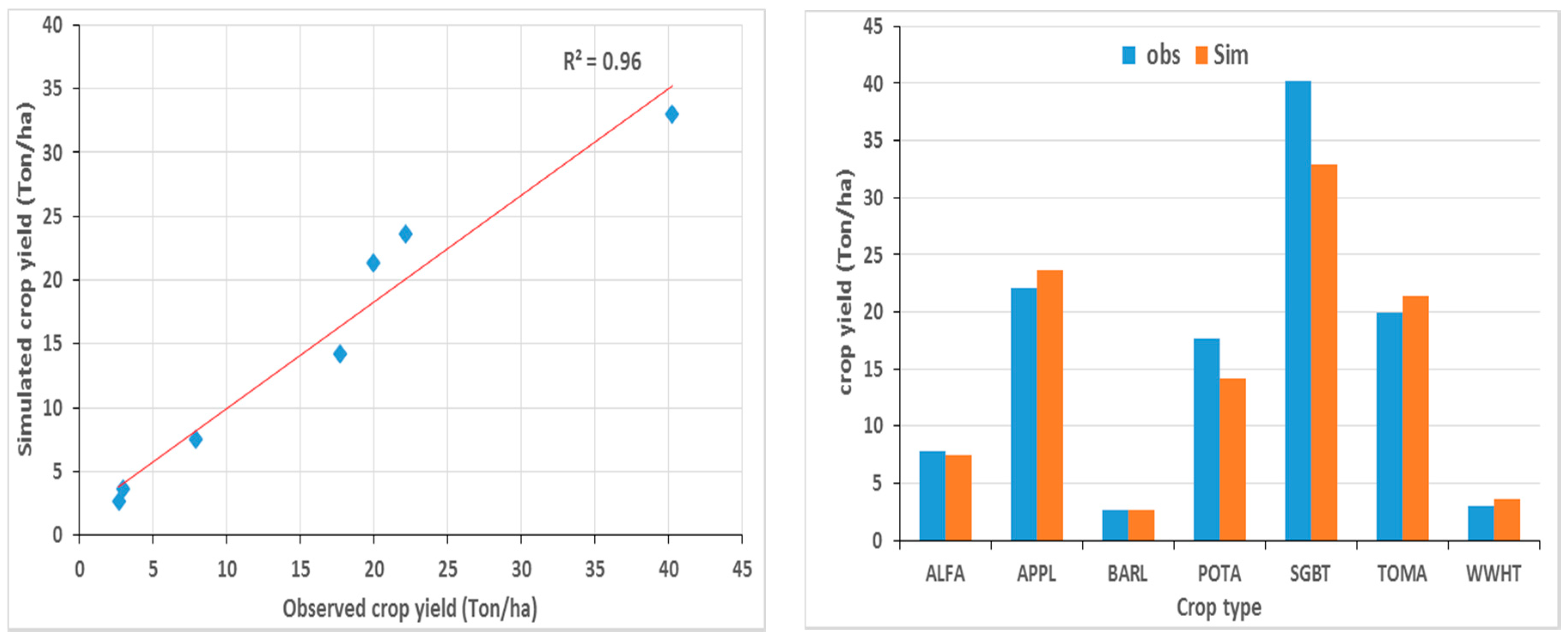
To do this, climate change in the ZRB is first predicted using a statistical downscaling method, two- step updated QM (Quantile Mapping) bias correction technique that is based on the most suitable GCM outputs for the min./max. temperatures and precipitation namely CGCM3 and CESM-CAM5 of CMIP5 archive to assess the impact scenarios of the climate change (RCP 4.5, 6.0, and 8.5) in three 19-years future periods (near, middle, and far). In the next step, the downscaled weather variables are applied to the calibrated and validated basin-wide hydrologic model, SWAT, to simulate the future available water resources including the reservoir inflow and hydrologic changes. The crop yield potentials are also simulated using the SWAT model with applying the irrigation depths based on their monthly crop water requirements and adjusting the crop parameters.

According to the predicted impacts of climate change, RCP60 an RCP85 are expected to have the highest increase and decrease, respectively, of the inflow to the Boukan Dam. For all RCPs, the Boukan Dam inflow will be increased in the near and middle future, in comparison with the minimum and the mean historical dam inflow, except for RCP45 in the near future, whereas it is predicted that they will decrease by 2% to 23% for the far future period. The lowest available water resources are predicted for the far future regarding rather low precipitation and high temperature, especially for RCP85, which has the highest decrease of freshwater. The performance of the SWAT model for the streamflow and the crop yield simulation is quite satisfactory. The ratio of water demand across the water supply, i.e., the WaSSI (water stress) indices of the ZRB-simulated scenarios are predicted to be higher than the historical period for the near and medium periods, while the highest water stress is expected for the far future period.

To set up a water planning simulation module, the MODSIM model is then customized to allocate the available water based on priority constraints set for the ZRB. Finally, the CSPSO-MODSIM hydro-economic simulation-optimization model is developed by coupling this customized MODSIM model with a Constrained SPSO optimization algorithm, wherefore the objective function is here the total net economic benefit (NEB_t)—which basically is the product of the total agro-economic water productivity (AEWP^t) and the total amount of water supplied Q_t-under the constraints of different cereal crop pattern scenarios and the total arable areas existent for the three irrigation plots considered, i.e., the Boukan Dam downstream irrigation network, the plot upstream of the dam, and the RK plain. A penalty function method is employed to convert the constrained optimization problem to an unconstrained one, which can then be solved while using the classical SPSO algorithm.

The results of the application of the hydro-economic CSPSO-MODSIM model indicate that the optimal total net economic benefit (NEB_t) from all major crops in the ZRB basin (not including APPL, which is grown in orchards and cannot easily be altered over the short run) can be improved by appropriate adjustments of the different crop cultivation areas from that of the historical period (32.2 Million USD), to 35.3 and 37.4 Million USD for the two medium emission scenarios RCP45 and RCP60, respectively, but remain invariant for the extreme RCP85 (32.6 Million USD), though with an average reduction of the agricultural water use Q of 38%.

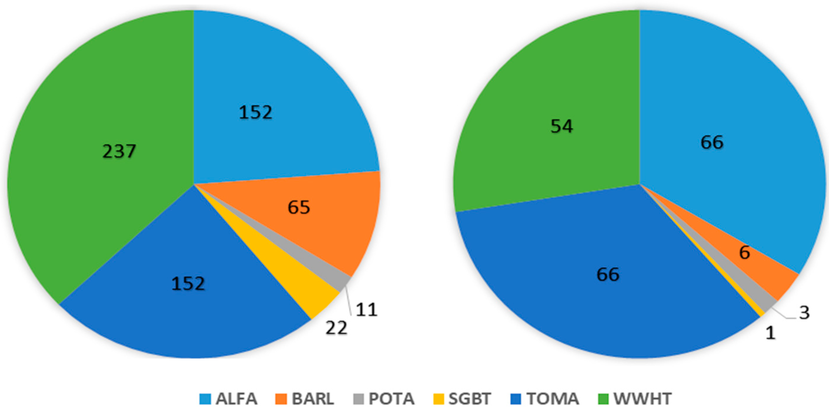
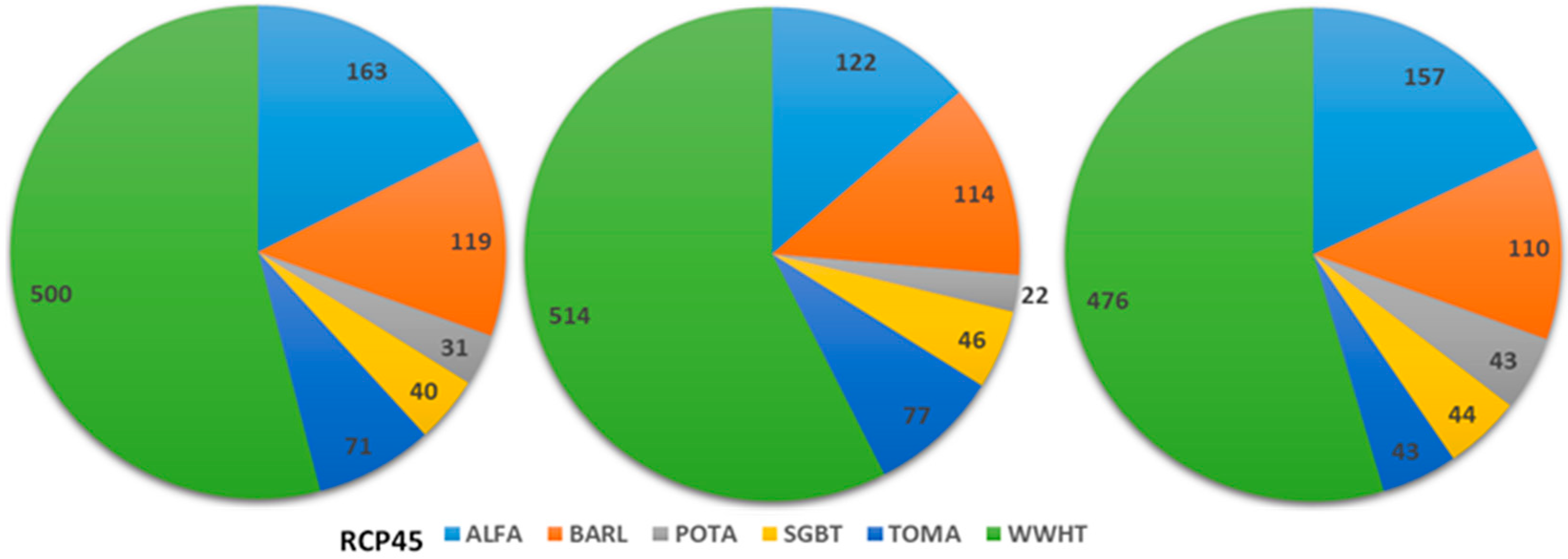
This overall increase of the future maximal NEB_t is based on optimal crop pattern areas as decision variables that hint of a significant extension of the total arable area from its historical value of 632 km² to up to 900 km², i.e., a relative increase that varies, depending on the future period/RCP, between 36% and 46% and so helps to guarantee the food security in the ZRB. Moreover, the strongest average increases of acreage of about 75%, amounting to an extension of approximately 250 km², are reserved for the strategic crops BARL and WWHT, owing to the 65%-devoted areal model constraint for these cereals and also to their rather high estimated AEWPs and low water demands Q.

However, this large extension of the two cereal acreages is made primarily at the expense of the crop area for ALFA, which, because of its low AEWP and rather high water demand, will be decreased by more than 30% in the future, so that it becomes economically more efficient to import portions of that crop from a neighbour catchment, such as the Aras River Basin.

POTA-, SGBT-, and TOMA-crop areas, in particular, will, relative to their historic values, also be also tremendously increased, though less in absolute numbers than those of the cereals above. In this vegetable group, the TOMA share of crop pattern exhibits the largest extension of about 250%, owing to its high water productivity (AEWP) and this holds for all three RCPs investigated. For the wetter RCP45- and RCP60-scenarios, the POTA- and SGBT-crop areas will, because of more available water, be doubled as well. On the other hand, for the most extreme RCP85-scenario, BARL- and SGBT-areal shares will augment by an average 85%, whereas the POTA-acreage will then have the lowest percentile increase of only 50%.

Thus, in summary, to improve the total net income from agriculture in the ZRB, it is recommended to replace the high-consuming water and low agro-economic water productivity crops, such as ALFA, APPL, and SGBT with crops of less water demand and higher economic benefits that, in addition to the other major crops of the ZRB investigated here (BARL, WWHT, TOMA, POTA) could be some new region-specific crops, such as canola, saffron, and pistachio, which all have high absolute selling prices and relatively high AEWPs.

In conclusion, the sequential SWAT-MODSIM-CSPSO hydro-economic optimization model developed here turns out to be an efficient tool for quantitative studies of agricultural economics and water resources management, namely, in semi-arid basins with agricultural cultivation under deficit irrigation. Moreover, by driving the model by future climate predictors, climate change impacts on agricultural productivity can be evaluated, and the latter eventually be optimized under the vagaries of climate change. Using a model, as the one proposed here, will allow water resources authorities and other stakeholders, not only in agriculture, to find the most suitable regional water- and land management strategies and optimal land-use planning scenarios for future years.

As a caveat, though, it may be noted that the accuracy of the present hydro-economic optimization model could be improved by implementing more sophisticated crop yield forecasting methods, such as to allow the estimation of different crop-yield response factors Ky_c for each stage of the crop growth; optimization of the crop production function; and, consideration of all the spatial and temporal changes of land use classes and their related water demands in the model.

References

1. OCHA, UN. Water Scarcity and Humanitarian Action: Key Emerging Trends and Challenges; UN. World Economic Forum,“Global Risks” (2014); UN: Washington, DC, USA, 2010. [Google Scholar]
2. Mo, X.-G.; Hu, S.; Lin, Z.-H.; Liu, S.-X.; Xia, J. Impacts of climate change on agricultural water resources and adaptation on the north china plain. Adv. Clim. Chang. Res. 2017, 8, 93–98. [Google Scholar] [CrossRef]
3. Voss, K.A.; Famiglietti, J.S.; Lo, M.; Linage, C.; Rodell, M.; Swenson, S.C. Groundwater depletion in the middle east from grace with implications for transboundary water management in the tigris-euphrates-western Iran region. Water Resour. Res. 2013, 49, 904–914. [Google Scholar] [CrossRef] [PubMed]
4. Dubois, O. The State of the World's Land and Water Resources for Food and Agriculture: Managing Systems at Risk; Earthscan: London, UK, 2011. [Google Scholar]
5. Mesgaran, M.B.; Madani, K.; Hashemi, H.; Azadi, P. Iran’s land suitability for agriculture. Sci. Rep. 2017, 7, 7670. [Google Scholar] [CrossRef] [PubMed]
6. Van Arendonk, A. The Development of the Share of Agriculture in GDP and Employment. Master’s Thesis, Wageningen University, Wageningen, The Netherlands, 2015. [Google Scholar]
7. Motamed, M. Developments in Iran’s Agriculture Sector and Prospects for US Trade; Economic Research Service/USDA: Washington, DC, USA, 2017. [Google Scholar]
8. Rafiei Emam, A. Impact of Climate and Land Use Change on Water Resources, Crop Production and Land Degradation in a Semi-arid Area (Using remote Sensing, GIS and Hydrological Modeling). Ph.D. Thesis, The Georg-August University School of Science (GAUSS), Göttingen, Germany, February 2015. [Google Scholar]
9. Conforti, P. Looking ahead in World Food and Agriculture: Perspectives to 2050; Food and Agriculture Organization of the United Nations (FAO): Rome, Italy, 2011. [Google Scholar]
10. Alexandratos, N.; Bruinsma, J. World Agriculture towards 2030/2050: The 2012 Revision; ESA Working Paper; FAO: Rome, Italy, 2012. [Google Scholar]
11. OECD. Achieving Sustainable Agricultural Productivity Growth. In OECD-FAO Agricultural Outlook; OECD Publishing: Paris, France, 2012. [Google Scholar]
12. Abbaspour, K.C.; Faramarzi, M.; Ghasemi, S.S.; Yang, H. Assessing the impact of climate change on water resources in Iran. Water Resour. Res. 2009, 45. [Google Scholar] [CrossRef] [Green Version]
13. Emami, F.; Koch, M. Evaluation of statistical-downscaling/bias-correction methods to predict hydrologic responses to climate change in the zarrine river basin, Iran. Climate 2018, 6, 30. [Google Scholar] [CrossRef]
14. Chijioke, O.B.; Haile, M.; Waschkeit, C. Implication of Climate Change on Crop Yield and Food Accessibility in Sub-Saharan Africa; Centre for Development Research, University of Bonn: Bonn, Germany, 2011. [Google Scholar]
15. Ashraf Vaghefi, S.; Mousavi, S.; Abbaspour, K.; Srinivasan, R.; Yang, H. Analyses of the impact of climate change on water resources components, drought and wheat yield in semiarid regions: Karkheh river basin in Iran. Hydrol. Process. 2014, 28, 2018–2032. [Google Scholar] [CrossRef]
16. Teshager, A.D.; Gassman, P.W.; Schoof, J.T. Assessment of impacts of agricultural and climate change scenarios on watershed water quantity and quality, and crop production. Hydrol. Earth Syst. Sci. 2016, 20, 3325. [Google Scholar] [CrossRef]
17. Bou-Fakhreddine, B.; Abou-Chakra, S.; Mougharbel, I.; Faye, A.; Pollet, Y. Optimal multi-crop planning implemented under deficit irrigation. In Proceedings of the 2016 18th Mediterranean Electrotechnical Conference (MELECON), Limassol, Cyprus, 18–20 April 2016; IEEE: Piscataway, NJ, USA, 2016; pp. 1–6. [Google Scholar]
18. Fazlali, A.; Shourian, M. A demand management based crop and irrigation planning using the simulation-optimization approach. Water Resour. Manag. 2018, 32, 67–81. [Google Scholar] [CrossRef]
19. Fredericks, J.W.; Labadie, J.W.; Altenhofen, J.M. Decision support system for conjunctive stream-aquifer management. J. Water Resour. Plan. Manag. 1998, 124, 69–78. [Google Scholar] [CrossRef]
20. Fereidoon, M.; Koch, M. SWAT-MODSIM-PSO optimization of multi-crop planning in the Karkheh river basin, Iran, under the impacts of climate change. Sci. Total Environ. 2018, 630, 502–516. [Google Scholar] [CrossRef] [PubMed]
21. Keshavarz, A.; Heydari, N.; Ashrafi, S. Management of agricultural water consumption, drought, and supply of water for future demands. In Proceedings of the Seventh International Conference on the Development of Dryland, Tehran, Iran, 14–17 September 2003; pp. 42–48. [Google Scholar]
22. Ahmadzadeh, H.; Morid, S.; Delavar, M.; Srinivasan, R. Using the swat model to assess the impacts of changing irrigation from surface to pressurized systems on water productivity and water saving in the zarrineh rud catchment. Agric. Water Manag. 2016, 175, 15–28. [Google Scholar] [CrossRef]
23. Grafton, R.Q.; Williams, J.; Perry, C.J.; Molle, F.; Ringler, C.; Steduto, P.; Udall, B.; Wheeler, S.A.; Wang, Y.; Garrick, D.; et al. The paradox of irrigation efficiency. Science 2018, 361, 748–750. [Google Scholar] [CrossRef] [PubMed]
24. ULRP. Challenges of Urmia Lake and Restoration Program. International Cooperation Division; Urmia Lake Restoration Program (ULRP); International Cooperation Division: Tehran, Iran, 2017. [Google Scholar]
25. Ministry of Agriculture (Agricultural Statistics and the Information Center). Available online: http://www.maj.ir/ (accessed on 30 June 2018).
26. Ministry of the Energy (MOE). Updating of Water Master Plan of Iran; Water and Wastewater Macro Planning Bureau: Tehran, Iran, 2014.
27. Ministry of Agriculture (MOA). Agriculture Statistics: Volume 1, Field Crops, Iranian Ministry of Agriculture (2014–2015); Ministry of Agriculture: Tehran, Iran, 2015.
28. Statistical Centre of Iran (SCI). Available online: www.amar.org.ir (accessed on 30 June 2018).
29. Harou, J.J.; Pulido-Velazquez, M.; Rosenberg, D.E.; Medellín-Azuara, J.; Lund, J.R.; Howitt, R.E. Hydro-economic models: Concepts, design, applications, and future prospects. J. Hydrol. 2009, 375, 627–643. [Google Scholar] [CrossRef] [Green Version]
30. Taylor, K.E.; Stouffer, R.J.; Meehl, G.A. An overview of CMIP5 and the experiment design. Bull. Am. Meteorol. Soc. 2012, 93, 485–498. [Google Scholar] [CrossRef]
31. Pachauri, R.K.; Allen, M.R.; Barros, V.R.; Broome, J.; Cramer, W.; Christ, R.; Church, J.A.; Clarke, L.; Dahe, Q.; Dasgupta, P. Climate Change 2014: Synthesis Report. Contribution of Working Groups I, II and III to the Fifth Assessment Report of the Intergovernmental Panel on Climate Change; IPCC: Geneva, Switzerland, 2014. [Google Scholar]
32. Hempel, S.; Frieler, K.; Warszawski, L.; Schewe, J.; Piontek, F. A trend-preserving bias correction—The isi-mip approach. Earth Syst. Dyn. 2013, 4, 219–236. [Google Scholar] [CrossRef]
33. Miao, C.; Su, L.; Sun, Q.; Duan, Q. A nonstationary bias-correction technique to remove bias in gcm simulations. J. Geophys. Res. Atmos. 2016, 121, 5718–5735. [Google Scholar] [CrossRef]
34. Neitsch, S.L.; Arnold, J.G.; Kiniry, J.R.; Williams, J.R. Soil and Water Assessment Tool Theoretical Documentation Version 2009; Texas Water Resources Institute: College Station, TX, USA, 2011. [Google Scholar]
35. Jha, M.; Pan, Z.; Takle, E.S.; Gu, R. Impacts of climate change on streamflow in the upper mississippi river basin: A regional climate model perspective. J. Geophys. Res. Atmos. 2004, 109. [Google Scholar] [CrossRef]
36. Abbaspour, K.C.; Johnson, C.; Van Genuchten, M.T. Estimating uncertain flow and transport parameters using a sequential uncertainty fitting procedure. Vadose Zone J. 2004, 3, 1340–1352. [Google Scholar] [CrossRef]
37. Krause, P.; Boyle, D.; Bäse, F. Comparison of different efficiency criteria for hydrological model assessment. Adv. Geosci. 2005, 5, 89–97. [Google Scholar] [CrossRef]
38. Moriasi, D.N.; Arnold, J.G.; Van Liew, M.W.; Bingner, R.L.; Harmel, R.D.; Veith, T.L. Model evaluation guidelines for systematic quantification of accuracy in watershed simulations. Trans. ASABE 2007, 50, 885–900. [Google Scholar] [CrossRef]
39. Abbaspour, K.C.; Yang, J.; Maximov, I.; Siber, R.; Bogner, K.; Mieleitner, J.; Zobrist, J.; Srinivasan, R. Modelling hydrology and water quality in the pre-alpine/alpine Thur watershed using SWAT. J. Hydrol. 2007, 333, 413–430. [Google Scholar] [CrossRef]
40. Srinivasan, R.; Zhang, X.; Arnold, J. Swat ungauged: Hydrological budget and crop yield predictions in the upper mississippi river basin. Trans. ASABE 2010, 53, 1533–1546. [Google Scholar] [CrossRef]
41. Vaghefi, S.A.; Mousavi, S.; Abbaspour, K.; Srinivasan, R.; Arnold, J. Integration of hydrologic and water allocation models in basin-scale water resources management considering crop pattern and climate change: Karkheh river basin in Iran. Reg. Environ. Chang. 2015, 15, 475–484. [Google Scholar] [CrossRef]
42. Evans, R.G.; Sadler, E.J. Methods and technologies to improve efficiency of water use. Water Resour. Res. 2008, 44. [Google Scholar] [CrossRef] [Green Version]
43. Zwart, S.J.; Bastiaanssen, W.G. Review of measured crop water productivity values for irrigated wheat, rice, cotton and maize. Agric. Water Manag. 2004, 69, 115–133. [Google Scholar] [CrossRef]
44. Molden, D.; Oweis, T.Y.; Steduto, P.; Kijne, J.W.; Hanjra, M.A.; Bindraban, P.S.; Bouman, B.A.M.; Cook, S.J.; Erenstein, O.; Farahani, H. Pathways for increasing agricultural water productivity. In Water for Food Water for Life: A Comprehensive Assessment of Water Management in Agriculture; Taylor and Francis AS: Abingdon, UK, 2007. [Google Scholar]
45. Labadie, J.W. MODSIM: Decision Support System for Integrated River Basin Management. In Proceedings of the 3rd International Congress on Environmental Modelling and Software, Burlington, VT, USA, 9–12 July 2006. [Google Scholar]
46. de Azevedo, L.G.T.; Gates, T.K.; Fontane, D.G.; Labadie, J.W.; Porto, R.L. Integration of water quantity and quality in strategic river basin planning. J. Water Resour. Plan. Manag. 2000, 126, 85–97. [Google Scholar] [CrossRef]
47. Morway, E.D.; Niswonger, R.G.; Triana, E. Toward improved simulation of river operations through integration with a hydrologic model. Environ. Model. Softw. 2016, 82, 255–274. [Google Scholar] [CrossRef]
48. Emami, F.; Koch, M. Evaluating the water resources and operation of the boukan dam in Iran under climate change. Eur. Water 2017, 59, 17–24. [Google Scholar]
49. Shourian, M.; Mousavi, S.; Tahershamsi, A. Basin-wide water resources planning by integrating PSO algorithm and MODSIM. Water Resour. Manag. 2008, 22, 1347–1366. [Google Scholar] [CrossRef]
50. Bertsekas, D.P.; Tseng, P. Partial proximal minimization algorithms for convex pprogramming. SIAM J. Optim. 1994, 4, 551–572. [Google Scholar] [CrossRef]
51. Kennedy, J.; Eberhart, R. PSO optimization. In Proceedings of the IEEE International Conference on Neural Networks, Perth, Australia, 27 November–1 December 1995; IEEE Service Center: Piscataway, NJ, USA, 1995; pp. 1941–1948. [Google Scholar]
52. Kennedy, J. The particle swarm: Social adaptation of knowledge. In Proceedings of the IEEE International Conference on Evolutionary Computation, Indianapolis, IN, USA, 13–16 April 1997; IEEE: Piscataway, NJ, USA, 1997; pp. 303–308. [Google Scholar]
53. Parsopoulos, K.E.; Vrahatis, M.N. Recent approaches to global optimization problems through particle swarm optimization. Nat. Comput. 2002, 1, 235–306. [Google Scholar] [CrossRef]
54. Parsopoulos, K.E.; Vrahatis, M.N. Particle swarm optimization method for constrained optimization problems. Intell. Technol. Theory Appl. New Trends Intell. Technol. 2002, 76, 214–220. [Google Scholar]
55. Eberhart, R.C.; Shi, Y. Comparison between genetic algorithms and particle swarm optimization. In Proceedings of the International Conference on Evolutionary Programming, San Diego, CA, USA, 25–27 March 1998; Springer: Berlin, Germany, 1998; pp. 611–616. [Google Scholar]
56. Clerc, M.; Kennedy, J. The particle swarm-explosion, stability, and convergence in a multidimensional complex space. IEEE Trans. Evolut. Comput. 2002, 6, 58–73. [Google Scholar] [CrossRef]
57. Stewart, J.I.; Robert, M. Functions to predict effects of crop water deficits. J. Irrig. Drain. Div. 1973, 99, 421–439. [Google Scholar]
58. Steduto, P.; Hsiao, T.C.; Fereres, E.; Raes, D. Crop Yield Response to Water; FAO: Rome, Italy, 2012; Volume 1028. [Google Scholar]
59. Alizadeh, A.; Kamali, G. Crops Water Requirements in Iran. Master’s Thesis, Emam Reza University, Mashhad, Iran, 2007. [Google Scholar]
60. Arnold, J.; Kiniry, J.; Sirinivasan, R.; Williams, J.; Haney, E.; Neitsh, S. Swat Input–Output Documentation, Version 2012; TR-439; Texas Water Resource Institute: College Station, TX, USA, 2012. [Google Scholar]
61. Naraqi, M.; Akbari, G.A.; Banihabib, M.E. Optimal crop pattern for Lake Urmia. In Proceedings of the First International and the Fourth National Conference of Iran’s Environmental and Agricultural Research, Hamedan, Iran, November 2015. [Google Scholar]
62. Ministry of the Energy. Executive Strategies for Decreasing 40% of Agricultural Water Demands in Zarrine and Simineh River Basins (Saeenghaleh and Miandoab Areas), Volume 7: Studies of Water Resources and Demands Planning and Management; Lake Urmia Restoration Committee: Urmia, Iran, 2016.
Figure 1. Map of the Zarrine River Basin (ZRB) with the Boukan Dam and the climate and streamflow stations.
Sustainability 10 03953 g001
Figure 2. Locations of irrigated croplands of the ZRB, Rahimkhan (RK) plain and the Boukan Dam.
Sustainability 10 03953 g002
Figure 3. Flowchart of the Constrained Stretched Particle Swarm Optimization (CSPSO)-MODSIM hydro-economic optimization model.
Sustainability 10 03953 g003
Figure 4. Schematics of the MODSIM model for the ZRB with related demand nodes, separated into three demand area groups, as indicated by the corresponding suffixes.
Sustainability 10 03953 g004
Figure 5. Spatial distributions of average 1987–2005 observed/bias corrected precipitation (left) and temperatures (right) in the ZRB.
Sustainability 10 03953 g005
Figure 6. Spatial distributions of average precipitation (top) and temperature (bottom) in the ZRB during the near future period (2020–2038) for three RCPs.
Sustainability 10 03953 g006
Figure 7. Similar to Figure 6, but for the middle future period (2050–2068).
Sustainability 10 03953 g007
Figure 8. Similar to Figure 6, but for the far future period (2080–2098).
Sustainability 10 03953 g008
Figure 9. Annual Soil Water Assessment Tool (SWAT)-simulated inflow to the Boukan Dam in the historical (1991–2012) and the three future periods, for the three RCPs, together with corresponding linear trend lines.
Sustainability 10 03953 g009
Figure 10. SWAT-simulated and observed average annual crop yields for 1987–2012. (Left panel) Linear regression; (Right panel) bar chart.
Sustainability 10 03953 g010
Figure 11. Current/historic crop pattern of the Boukan Dam (downstream) network—(left pie) and the dam upstream demand area (right pie) in km2.
Sustainability 10 03953 g011
Figure 12. Optimal crop pattern for RCP45 for the three future periods: the near (left panel), middle (middle panel) and far (right panel) future in km2.
Sustainability 10 03953 g012
Figure 13. Similar to Figure 8, but for RCP60.
Sustainability 10 03953 g013
Figure 14. Similar to Figure 11, but for RCP85.
Sustainability 10 03953 g014